


1. Introduction
Phoretic particles (rigid particles or drops) have recently been attracting an increased interest theoretically, numerically and experimentally (Michelin, Lauga & Bartolo Reference Michelin, Lauga and Bartolo2013; Schmitt & Stark Reference Schmitt and Stark2013; Izri et al. Reference Izri, Van Der Linden, Michelin and Dauchot2014; Michelin & Lauga Reference Michelin and Lauga2014; Jin, Krüger & Maass Reference Jin, Krüger and Maass2017; Hu et al. Reference Hu, Lin, Rafai and Misbah2019; Morozov & Michelin Reference Morozov and Michelin2019a,Reference Morozov and Michelinb; Izzet et al. Reference Izzet, Moerman, Gross, Groenewold, Hollingsworth, Bibette and Brujic2020; Morozov Reference Morozov2020; Chen et al. Reference Chen, Chong, Liu, Verzicco and Lohse2021; Hokmabad et al. Reference Hokmabad, Dey, Jalaal, Mohanty, Almukambetova, Baldwin, Lohse and Maass2021). In its simplest version, the model consists of a particle that emits or absorbs (with an emission/absorption rate  $A$) a solute which diffuses, with bulk diffusion constant
 $D$, and is advected by the suspending fluid. The interaction between the solute and the particle can be shown (Michelin & Lauga Reference Michelin and Lauga2014) to result in a tangential flow along the particle, in the form of (in the frame moving with particle)
 ${\boldsymbol {V}} = M \nabla _s c$, where
 ${\boldsymbol {V}}$ is the velocity,
 $c$ the solute concentration,
 $\nabla _s$ is the gradient along the particle surface, and
 $M$ is a mobility factor involving fluid viscosity and the interaction potential between the solute and the particle. This problem can be characterized by a Péclet number
 $Pe=AM a/D^2$ where
 $a$ is the particle radius. The solute concentration
 $c({\boldsymbol {r}},t)$ (where
 ${\boldsymbol {r}}$ is a position in space and
 $t$ is time) and velocity
 ${{\boldsymbol {V}}} ({\boldsymbol {r}}, t)$ obey the advection–diffusion and the Stokes equations. It has been shown analytically, from a linear stability analysis, both in two dimensions (Hu et al. Reference Hu, Lin, Rafai and Misbah2019) and three dimensions (Michelin et al. Reference Michelin, Lauga and Bartolo2013) that if
 $Pe\ge Pe_1$ (where
 $Pe_1$ is a critical number), the particle undergoes a bifurcation from a non-motile state (swimming velocity
 ${V}_0=0$) into a motile state (
 ${V}_0\ne 0$). A linear stability analysis only informs us of the instability onset from one state to another, but is not sufficient to describe how the velocity behaves with
 $Pe$, where a nonlinear analysis is needed. Numerical simulations (Michelin et al. Reference Michelin, Lauga and Bartolo2013; Hu et al. Reference Hu, Lin, Rafai and Misbah2019) seemed consistent with the fact that
 ${V}_0$ is well represented by
 ${V}_0 \sim \pm (Pe-Pe_1)^{1/2}$ in the vicinity of the bifurcation point; the solution
 ${V}_0=0$ always exists, and is stable for
 $Pe< Pe_1$ and becomes unstable for
 $Pe>Pe_1$, in favour of two stable branches of solutions
 ${V}_0 \sim \pm (Pe-Pe_1)^{1/2}$. This is a classical pitchfork bifurcation (see the Conclusion for the occurrence of a singular pitchfork bifurcation). Numerical simulations in two dimensions (Hu et al. Reference Hu, Lin, Rafai and Misbah2019) also showed that by increasing
 $Pe$ further the straight moving solution becomes unstable in favour of various states (meandering, circular and chaotic solutions). Simulations in three dimensions under an axisymmetric constraint (imposing to the particle to move along a line) also reported (Morozov & Michelin Reference Morozov and Michelin2019a) on chaotic solutions (the particle goes back and forth in a chaotic manner). Relaxing the axisymmetric constraint in three dimensions also revealed, among other motion, meandering and chaotic motion in the form of a persistent random walk (Hu et al. Reference Hu, Lin, Rafai and Chaouqi2022). The transition from a non-motile to a motile state, as well as irregular motion (apparently chaotic) has also been reported experimentally (Izri et al. Reference Izri, Van Der Linden, Michelin and Dauchot2014; Jin et al. Reference Jin, Krüger and Maass2017; Izzet et al. Reference Izzet, Moerman, Gross, Groenewold, Hollingsworth, Bibette and Brujic2020; Hokmabad et al. Reference Hokmabad, Dey, Jalaal, Mohanty, Almukambetova, Baldwin, Lohse and Maass2021), and in some numerical simulations (Chen et al. Reference Chen, Chong, Liu, Verzicco and Lohse2021). The transition from a non-motile to a motile state also takes place in the presence of a Marangoni stress (Izri et al. Reference Izri, Van Der Linden, Michelin and Dauchot2014; Morozov & Michelin Reference Morozov and Michelin2019a). In a completely different context, that of cell motility driven by acto-myosin, rich dynamics (transition from a motile to a non-motile state, Hopf bifurcation, etc.) have also been reported when the activity of the cell (represented by myosin contractility) exceeds a certain critical value (Hawkins et al. Reference Hawkins, Poincloux, Bénichou, Piel, Chavrier and Voituriez2011; Callan-Jones et al. Reference Callan-Jones, Ruprecht, Wieser, Heisenberg and Voituriez2016; Farutin et al. Reference Farutin, Etienne, Misbah and Récho2019).
The above non-trivial behaviours have been obtained in most cases by numerical simulations of model equations involving diffusion and advection with a moving boundary. It is thus highly desirable to see whether or not these features can be translated into a more universal language, since we expect the form of the reduced model equations not to depend on a specific phoretic model. One way is to look for a reductive perturbative scheme that allows one to extract equations from the full model, which are prototypical simplified equations (their form does not depend on the considered swimmer model). By starting from the phoretic model described above, we will extract, by following a nonlinear perturbative scheme, two coupled (weakly nonlinear) equations for the time evolution of the complex amplitudes of the first two Fourier modes, while the spatial dependence can be handled analytically. These equations will enable us to analyse, besides the first (primary) bifurcation (transition from a motile to a non-motile state), a secondary bifurcation corresponding to a transition from straight to circular trajectories. We will also exemplify its power in capturing irregular motion. In the same spirit, Li (Reference Li2022) has extracted a reduced model from the same phoretic model, by considering only the first harmonic. This calculation could account only for the transition from a motionless state to a straight motion, in the form of a pitchfork bifurcation. In that paper, a finite size was adopted, as done here, in order to avoid divergence of concentration field. Restricting the reduced model to the first harmonic cannot account for complex motions (e.g. circular trajectory and chaos). We will see that including the first and second harmonics will capture these complex features, but also provides quantitative agreement with the full simulation. It will be seen that including the second harmonic to the desired order of expansion is far from being trivial, and this requires several mathematical subtleties.
We will exemplify the method for a two-dimensional (2-D) model (for simplicity), but the technique should work perfectly well in three dimensions. In our calculation, we will also see that the method can be readily adapted to other phoretic models (for example by taking into account a consumption term, or having different boundary conditions). Indeed most of our calculations do not rely on the explicit form of the evolution equations for the concentration field, highlighting the general feasibility of the approach. It is only when the explicit expressions of the coefficients are derived that the explicit form of the operator (and its eigenfunctions) is used. In the case where eigenfunctions cannot be obtained analytically for another swimming problem, they can always be tabulated as integrals, but the reduced model (in terms of the first two Fourier modes) will keep the same form. This will be discussed in more detail in the main text.
2. Problem formulation
Our starting point is a simple phoretic model in two dimensions. Figure 1 shows the geometry of the considered system. In two dimensions we will see that the concentration field diverges at  $\infty$, this is why the domain for the concentration field is taken to be finite having extent
 $r=R$ (see figure 1). Another possibility to obtain a steady-state concentration field is to introduce chemical consumption proportional to the local concentration. This additional effect results in steady-state solutions that show asymptotically an exponential decay at large distances from the particle, where the characteristic length scale of the decaying field is given by a competition of the diffusion and chemical consumption processes. Setting the finite size of the domain for the concentration field, while keeping the flow domain infinite, can thus be seen as a qualitative approximation of the consumption model in an infinite domain, where the exponential decay is replaced by a sharp external boundary. Here we prefer to use the finite domain for the concentration field because this boundary condition allows us to complete all calculations symbolically. The concentration field in the consumption model can only be expressed in terms of cylindrical Bessel functions, which would oblige us to use numerical solutions to obtain the coefficients of the reduced model equations.
The particle has radius  $a$, and the fluid as well as the concentration fields are defined between the particle periphery
 $r=a$ and external boundary
 $r=R$.

We first recall the problem formulation (Michelin et al. Reference Michelin, Lauga and Bartolo2013; Michelin & Lauga Reference Michelin and Lauga2014). The concentration field  $c(\boldsymbol {r},t)$ subject to an advection–diffusion equation outside the particle
 \begin{equation} \partial_t c(\boldsymbol{r},t)=D\nabla^2 c(\boldsymbol{r},t)- \boldsymbol{\nabla}\boldsymbol{\cdot} [c(\boldsymbol{r},t) \boldsymbol{V}(\boldsymbol{r},t)], \end{equation}
where the advection velocity field  $\boldsymbol {V}(\boldsymbol {r},t)$ in the comoving frame is obtained by solving the Stokes equations in the fluid outside the particle
 \begin{equation} {-}\boldsymbol{\nabla} p + \eta \Delta \boldsymbol{V} = \boldsymbol{0}, \quad \boldsymbol{\nabla}\boldsymbol{\cdot} \boldsymbol{V}= 0, \end{equation}
where  $p$ is the pressure field and
 $\eta$ is the fluid viscosity. Here the 2-D position vector
 $\boldsymbol {r}$ is measured relative to the particle centre and
 $D$ is the diffusion coefficient. We use polar coordinates
 $(r,\phi )$, centred at the particle position in the following derivation. The boundary conditions for the concentration field read
 \begin{equation} \partial_rc(\boldsymbol{r},t)|_{r=a}={-}A/D, \quad c(\boldsymbol{r},t)|_{r=R}=0, \end{equation}
where  $a$ is the particle size and
 $R$ is the system size. The flow velocity satisfies the following boundary conditions:
 \begin{equation} \boldsymbol{V}(\boldsymbol{r},t)|_{r=\infty}={-}\boldsymbol{V}_0(t),\quad \boldsymbol{V}(\boldsymbol{r},t)|_{r=a}={M} \boldsymbol \nabla^s c(\boldsymbol{r},t)|_{r=a}, \end{equation}
where  $\boldsymbol {V}_0(t)$ is the swimming speed of the particle (undetermined for the moment),
 $\boldsymbol {\nabla }^s$ is the surface gradient operator and
 $M$ is the particle mobility. The system is closed by requiring the net force acting on the particle to be zero, which allows one to compute the swimming velocity
 $V_0(t)$.
We will use the following dimensionalization. We use  $a$ as the unit of length,
 $a^2/D$ as the unit of time,
 $aA/D$ as the unit of concentration and
 $\eta D/a^2$ as the unit of pressure. The set of equations reduce to (by keeping the same symbols for concentration, velocity and pressure)
 $$\begin{gather} \partial_t c(\boldsymbol{r},t)=\nabla^2 c(\boldsymbol{r},t)-\boldsymbol{\nabla}\boldsymbol{\cdot} [c(\boldsymbol{r},t)\boldsymbol{V}(\boldsymbol{r},t)], \end{gather}$$
 $$\begin{gather}-\boldsymbol{\nabla} p + \Delta \boldsymbol{V} = \boldsymbol{0}, \quad \boldsymbol{\nabla}\boldsymbol{\cdot} \boldsymbol{V}= 0, \end{gather}$$
 $$\begin{gather}\partial_rc(\boldsymbol{r},t)|_{r=1}={-}1,\quad c(\boldsymbol{r},t)|_{r=R}=0, \end{gather}$$
 $$\begin{gather}\boldsymbol{V}(\boldsymbol{r},t)|_{r=\infty}={-}\boldsymbol{V}_0(t), \quad \boldsymbol{V}(\boldsymbol{r},t)|_{r=1}=Pe\boldsymbol \nabla^s c(\boldsymbol{r},t)|_{r=1}. \end{gather}$$
The remaining two non-dimensional numbers are  $Pe=AMa/D^2$ (Péclet number) and system size
 $R/a$, denoted as
 $R$.
It is conventional to express the fluid velocity in terms of the stream function  $\psi$:
 \begin{equation} V_r(\boldsymbol{r},t)=\frac{\partial_\phi \psi(\boldsymbol{r},t)}{r},\quad V_\phi(\boldsymbol{r},t)={-} \partial_r \psi(\boldsymbol{r},t). \end{equation}
The stream function is related to the concentration distribution along the particle boundary by the boundary condition (2.4a,b), as explained below.
3. Expansion in Fourier harmonics
Following the previous works (Michelin et al. Reference Michelin, Lauga and Bartolo2013; Hu et al. Reference Hu, Lin, Rafai and Misbah2019), the concentration field and the stream function are expanded in Fourier harmonics of the polar angle  $\phi$:
 \begin{equation} c(\boldsymbol{r},t)=\sum_{l={-}\infty}^\infty c_l(r,t)\, {\rm e}^{{\rm i}l\phi}, \quad \psi(\boldsymbol{r},t)=\sum_{l={-}\infty}^\infty \psi_l(r,t) \, {\rm e}^{{\rm i}l\phi}, \end{equation}
where we have  $c_l(r)=c_{-l}(r)^*$ and
 $\psi _l(r)=\psi _{-l}(r)^*$ as requirements for
 $c$ and
 $\psi$ to be real. We first determine the stream function. It is convenient to define it as a vector
 $\boldsymbol {\psi }=\psi \hat e_z$, where
 $\hat e_z$ is the unit vector along the
 $z$ coordinate in cylindrical coordinates. Equation (2.9a,b) can be written as
 $\boldsymbol {V}=\boldsymbol {\nabla } \times \boldsymbol {\psi }$. Taking the curl of the first (2.6a,b), we easily find (using the identity
 $\boldsymbol {\nabla } \times \boldsymbol {\nabla } \times \boldsymbol {\psi }=\boldsymbol {\nabla } (\boldsymbol {\nabla } \boldsymbol {\cdot } \boldsymbol {\psi }))- \nabla ^2 \boldsymbol {\psi }$), that the scalar
 $\psi$ obeys a biharmonic equation
 $\nabla ^4 \psi =0$. Using the decomposition (3.1a,b) we easily find the radial dependence for a physically acceptable solution
 $\psi _l(r,t)= \alpha _1 / r^{|l|}+ \alpha _2/ r^{|l|-2}$ where
 $\alpha _i$ are integration constants. These constants are determined from the second boundary condition (2.4a,b), yielding easily
 \begin{equation} \psi_l(r)=\frac{ilPe(1-r^2)}{2r^{|l|}}c_l(1). \end{equation}
Exploiting the force-free condition on the particle, the swimming velocity is obtained as (Hu et al. Reference Hu, Lin, Rafai and Misbah2019)
 \begin{equation} V_{0x}={-}Pe{\rm Re} c_1(1), \quad V_{0y}=Pe{\rm Im} c_1(1). \end{equation}
The advection–diffusion equation (2.1) is expanded in Fourier harmonics as
 \begin{equation} \partial_t c_l(r)=\hat D_l c_l(r)-[\boldsymbol{\nabla} \boldsymbol{\cdot}(c(\boldsymbol{r})\boldsymbol{V} (\boldsymbol{r}))]_l, \end{equation}
where  $\hat D_l$ is the diffusion operator applied to the
 $l$th Fourier harmonic,
 \begin{equation} \hat D_l=\frac{1}{r}\partial_r(r\partial_r)-\frac{l^2}{r^2}, \end{equation}
and  $[\boldsymbol {\nabla }\boldsymbol {\cdot }(c(\boldsymbol {r})\boldsymbol u(\boldsymbol {r}))]_l$ is the
 $l$th Fourier harmonic of the advection term.
4. Stationary state and linear approximation
The linear stability of the isotropic solution was already analysed in previous works in three dimensions (Michelin et al. Reference Michelin, Lauga and Bartolo2013) and in two dimensions (Hu et al. Reference Hu, Lin, Rafai and Misbah2019). Nevertheless, we present it briefly as the first step of the solution of the nonlinear problem. The isotropic solution corresponds to
 \begin{equation} {c_0(r,t)}=c_0(r)={-}\ln\frac{r}{R}. \end{equation}
We insert expression (3.1a,b) into the advection–diffusion equation (2.5). The only nonlinear term is the last one. In the linear regime it reads  $\sum _\ell V_{r\ell }(r) \partial _r c_0(r) \, {\rm e}^{{\rm i}\ell \phi }$ (the zeroth order of velocity field is zero because the unperturbed state is the stationary particle, so that the fluid is quiescent to leading order). We then make use of (4.1) for
 $c_0(r)$ and (2.9a,b) for
 $V_{r\ell }$, by exploiting (3.2). All these together allow one to obtain from (2.5) the following evolution equation for
 $c_l$:
 \begin{equation} \partial_t c_l(r)=\hat L_l(Pe) c_l(r)= \hat D_l c_l(r)+Pe u_l(r)c_l(1), \end{equation}
where  $\hat L_l{(Pe)}$ is the linear stability operator for the
 $l$th harmonic for given
 $Pe$, and we have defined
 \begin{equation} u_l(r)=\frac{l^2(r^2-1)}{2r^{l+2}}. \end{equation}
This velocity contribution stems from the radial contribution of  $\boldsymbol {V}$, but we will omit the
 $r$ subscript in
 $u_\ell$ since only this contribution enters the linear operator, and this will be used as a definition of this
 $r$-dependent function without any ambiguity in what follows.
The linear stability of the isotropic solution is governed by the eigenvalues  $\lambda _{l,k}{(Pe)}$ of the operators
 $\hat L_l{(Pe)}$, defined as
 \begin{equation} \hat L_l (Pe)f_{l,k}(r{,Pe})=\lambda_{l,k}{(Pe)}f_{l,k}(r{,Pe}), \end{equation}
where  $f_{l,k}(r{,Pe})$ are the corresponding proper functions for given
 $Pe$. The subscript
 $l$ is associated with the
 $\phi$ variable and
 $k$ with the
 $r$ one. We index the eigenvalues for given
 $l$ in descending order with respect to their real part, starting with
 $\lambda _{l,0}{(Pe)}\equiv \lambda _l{(Pe)}$, which corresponds to the most unstable mode. It is essential for our analysis to assume the eigenvalue spectrum to be discrete, which is the case for a finite domain. In general, neither the eigenvalues nor the proper functions of
 $\hat L_l(Pe)$ have an elementary expression. However, it is known that for each
 $l\ge 1$, there is exactly one critical Péclet number
 $Pe_l$ such that the operator
 $\hat L_l(Pe_l)$ has an eigenvalue equal to zero (Michelin & Lauga Reference Michelin and Lauga2014; Hu et al. Reference Hu, Lin, Rafai and Misbah2019). Both
 $Pe_l$ (i.e.
 $Pe_1$ and
 $Pe_2$) as a function of
 $R$ and the proper function of
 $\hat L_l(Pe_l)$ corresponding to the zero eigenvalue have an explicit expression in elementary functions, given below.
For low enough  $Pe$, the eigenvalues of
 $\hat L_l(Pe)$ are close to those of the diffusion operator
 $\hat D_l$ and are thus all negative. The isotropic solution is stable in this case (growth rate of all modes is negative for all
 $l$). As
 $Pe$ increases, one of the proper values for given
 $l$ (
 $\lambda _{l,0}{(Pe)}\equiv \lambda _l{(Pe)}$) becomes equal to zero at
 $Pe=Pe_l$ and positive for
 $Pe>Pe_l$. Thus
 $Pe_l$ is found from
 \begin{equation} \lambda_l(Pe_l)=0. \end{equation}
The corresponding proper function  $f_{l,0}(r{,Pe_l})\equiv f_l(r)$ defines the perturbation mode that becomes unstable at
 $Pe=Pe_l$. Here and after we drop the eigenvalues and eigenfunctions for the
 $l$th harmonic taken at
 $Pe=Pe_l$ will be referred to without mentioning the value of
 $Pe$ explicitly:
 $\lambda _{l,k}\equiv \lambda _{l,k}(Pe_l)$,
 $f_{l,k}(r)\equiv f_{l,k}(r,Pe)$. The linear stability analysis allows us to determine the angular dependence (given by
 $l$ corresponding to the lowest
 $Pe_l$) and the radial dependence (given by
 $f_l(r)$) of the solution in the anisotropic phase. Further analysis is performed by a higher-order perturbation expansion in order to compute the swimming speed and the angular velocity of the particle in the anisotropic phase, as explained below.
Here we exclude the possibility of transition to an anisotropic concentration distribution by a Hopf bifurcation. Since the operators  $\hat L_l(Pe)$ are not self-adjoint, their proper values can be complex. It is therefore possible for the isotropic solution to become unstable due to one of the complex eigenvalues seeing its real part become positive. We exclude this possibility based on the results of full numerical simulations, shown below.
5. Weakly nonlinear expansion
This section presents the derivation of the weakly nonlinear equations governing the particle dynamics. A linear stability analysis has been already performed in two dimensions (Hu et al. Reference Hu, Lin, Rafai and Misbah2019), relating the growth rate  $\sigma _\ell$ of the instability for each
 $\ell$-harmonic, as a function of
 $Pe$ and system size
 $R$. To make the calculation consistent, we will look for conditions where the first and second harmonics are close to criticality (by tuning
 $R$ and
 $Pe$), while all other harmonics correspond to stable modes. The critical Péclet numbers for the first two harmonics where their growth rates
 $\sigma _1$ and
 $\sigma _2$ vanish are denoted as
 $Pe_1$ and
 $Pe_2$, respectively. This means (Hu et al. Reference Hu, Lin, Rafai and Misbah2019) that
 $\sigma _\ell \sim (Pe-Pe_\ell )\sim \epsilon$ (which defines a small parameter). In the vicinity of the instability
 $(Pe-Pe_\ell )$ is small and we introduce an expansion parameter
 $\epsilon$ expressing this smallness. Because we require that
 $Pe_1\sim Pe_2$, we search for a critical value of
 $R$ where this condition is fulfilled. We find that
 $Pe_1$ becomes equal to
 $Pe_2$ at
 $R=R_c$, where
 $R_c=3.17493$. We thus have to assume that
 $R=R_c+O(\epsilon )$, but also
 $R>R_c$, the second condition guaranteeing
 $Pe_1< Pe_2$. Here
 $\epsilon$ is the small parameter with respect to which the perturbation expansion is made. With these assumptions,
 $c=c_0(r)$ is the only stable possible solution for
 $Pe< Pe_1$. This solution becomes unstable at
 $Pe=Pe_1$ and a straight motion is expected to emerge at this point. At some value of
 $Pe$ between
 $Pe_1$ and
 $Pe_2$, the straight motion is expected to become unstable in favour of a circular motion (Hu et al. Reference Hu, Lin, Rafai and Misbah2019). Close to instability the amplitudes of concentrations corresponding to the first two harmonics are small, and are assumed to be of order
 $\epsilon$. In the linear regime we have
 $\dot C_1(t)=\sigma _1 C_1(t)$ and
 $\dot C_2(t)=\sigma _2 C_2(t)$, where
 $C_1$ and
 $C_2$ correspond to the amplitudes of the first two harmonics that are close to instability and depend on time only (by means of variable splitting the space dependence in the linear regime can be scaled out). Since
 $\sigma _\ell, C_\ell \sim \epsilon$, we can see that formally time derivative scales as
 $\epsilon$ (usual slowing down at a critical point). This means, for consistency, that the next nonlinear terms must be of the same order as the linear ones. Due to the assumed scaling of
 $C_\ell \sim \epsilon$ the first nonlinear terms balancing the linear ones, which must be of order
 $\sigma _\ell \sim \epsilon ^2$, can be of the form
 $C_1^2$,
 $C_2^2$ and
 $C_1C_2$ (and possible combinations with complex conjugates). The expansion must then be made up to order
 $\epsilon ^2$ at least. We have been able to compute the
 $O(\epsilon ^2)$ terms analytically for an arbitrary value of
 $R$ and also all
 $O(\epsilon ^3)$ terms for a given numerical value of
 $R$. This is sufficient to reproduce quantitatively the straight and circular motions, as shown below. Our reduced model accounts also for irregular motions, reported in Hu et al. (Reference Hu, Lin, Rafai and Misbah2019).
5.1. General strategy
The goal of this derivation is to reduce the full dynamics of the autophoretic particle to a simplified system of ordinary differential equations for two complex variables,  $C_1(t)$ and
 $C_2(t)$ (depending only on time), where
 $C_1$ is the amplitude of the first harmonic and
 $C_2$ is the amplitude of the second harmonic in the concentration field. The main challenge is that in general, each Fourier harmonic
 $c_l$ of the concentration field is a function of the distance from the centre of the particle
 $r$. There is thus no straightforward way to represent the whole function
 $c_l$ by a single scalar variable. We overcome this problem by decomposing the functions
 $c_1(r)$ and
 $c_2(r)$, and
 $c_l(r)$ (for
 $l>2$) as
 \begin{equation} c_l(r,t)=C_l(t)f_l(r)+\delta c_l(r,t) \ l\in\{1,2\},\quad c_l(r,t)=\delta c_l(r,t) l\not\in\{1,2\}, \end{equation}
where  $C_l(t)$ is the complex amplitude,
 $f_l(r)$ is the proper function such that
 $\hat L_l(Pe_l) f_l(r)=0$, and
 $\delta c_l(r,t)$ is a projection of the function
 $c_l(r,t)$ on the space of all other proper functions of the operator
 $\hat L_l(Pe_l)$:
 \begin{equation} \delta c_l(r,t)=\sum_{k>0}C_{l,k}(t)f_{l,k}(r). \end{equation}
The decomposition (5.1a,b) is made using the proper functions of  $\hat L_l(Pe_l)$ even for
 $Pe\ne Pe_l$. It is assumed, as usual, that the eigenfunctions
 $f_{l,k}$ constitute a complete basis. This assumption will be justified by the fact that the reduced model consistently reproduces the results of the full numerical solution. Note that the general strategy which follows is not limited to a special form of the linear operator
 $\hat L_l(Pe_l)$. The linear operator can be quite general, meaning that the theory is valid for other phoretic models (for example including a consumption of the concentration field, or changing the particle to a droplet moving under self-sustained Marangoni effect). This is why we postpone the application to our phoretic model to § 7, where the corresponding eigenfunctions will be defined. This means that all what is presented in the sections preceding § 7 has a general validity.
For  $Pe< Pe_l$ or
 $Pe$ close to
 $Pe_l$, the eigenvalues corresponding to the functions
 $f_{l,k}{(r,Pe)}$ with
 $k>0$ all have negative real parts. Therefore, the relaxation time scale of the amplitudes
 $C_{l,k}(t)$ is defined by the absolute values of
 $\lambda _{l,k}{(Pe)}$ for
 $k>0$. Since the set of
 $\lambda _{l,k}$ is discrete and we have assumed
 $\lambda _{l,k}$ to be ordered decreasingly, the longest relaxation time scale is defined by
 $|\lambda _{l,1}{(Pe)}|{^{-1}=|\lambda _{l,1}{(Pe_l)}|^{-1}+O(|Pe-Pe_l|)}$. The relaxation time of the
 $f_l{(r,Pe)}$ mode scales as
 $1/|Pe-Pe_l|$ for
 $Pe$ close to
 $Pe_l$, which determines the main time scale of the dynamics close to the critical point. We thus have been able to re-express the functions
 $\delta c_l(r,t)$ as a nonlinear function of
 $C_1$ and
 $C_2$, with
 $r$-dependent coefficients. This is done by adiabatic elimination, as explained below. Since the eigenvalues and the proper functions of the operator
 $\hat L_l(Pe_l)$ do not have an elementary expression, the following procedure relies on the adiabatic elimination of the amplitude
 $\delta c_l(r,t)$ as a function, instead of eliminating each amplitude
 $C_{l,k}$ separately.
A similar strategy is employed to compute the  $r$ dependence of the amplitude of the other Fourier harmonics
 $c_l(r,t)$ for
 $l\not \in \{1,2\}$ as a function of
 $C_1$ and
 $C_2$, as also explained below. This will allow us to show that the whole concentration field
 $c(r,\phi,t)$ can be re-expressed as a perturbation expansion in powers of
 $C_1$ and
 $C_2$ after an initial transient relaxation. We present below a procedure to compute the coefficients of this expansion as explicit functions of
 $r$ and
 $\phi$.
5.2. Perturbation expansion
According to the discussion at the beginning of this section, we consider two coupled harmonics close to their instability threshold, which results in scaling  $C_1=O(\epsilon )$ and
 $C_2=O(\epsilon )$. The consistency of the evolution equations requires us to admit the following assumptions:
 $|Pe-Pe_1|=O(\epsilon )$;
 $|Pe-Pe_2|=O(\epsilon )$;
 $\partial _t C_1=O(\epsilon ^2)$;
 $\partial _t C_2=O(\epsilon ^2)$;
 $\delta c_1(r,t)=O(\epsilon ^2)$;
 $\delta c_2(r,t)=O(\epsilon ^2)$;
 $\partial _t\delta c_1(r,t)=O(\epsilon ^3)$;
 $\partial _t\delta c_2(r,t)=O(\epsilon ^3)$;
 $\delta c_0(r,t)=O(\epsilon ^2)$;
 $\partial _t \delta c_0(r,t)=O(\epsilon ^3)$. For
 $l>2$, we have
 $\delta c_{l}(r,t)=O(\epsilon ^{\lceil l/2\rceil })$ and
 $\partial _t \delta c_{l}(r,t)=O(\epsilon ^{\lceil l/2\rceil +1})$. The smallness of
 $\partial _t$ is due to the critical slowing down at the bifurcation point.
5.3. Adiabatic elimination
The problem requires us to reduce the partial derivative equations for functions  $c_l(r)$ to ordinary differential equations of two scalar amplitudes
 $C_1$ and
 $C_2$. This is performed by applying adiabatic elimination, as explained in this section.
First, we introduce the right proper function  $g_l$ of the operator
 $\hat L_l(Pe_l)$ such that the corresponding eigenvalue is zero,
 \begin{equation} \hat L_l^+(Pe_l) g_l(r)=0, \end{equation}
where  $\hat L_l(Pe_l)^+$ is the adjoint operator of
 $\hat L_l(Pe_l)$. The adjoint operator is defined with respect to the inner product
 \begin{equation} {\langle g,f\rangle}=\int_1^R f(r)g(r)^* r\, {\rm d} r, \end{equation}
which is chosen to maintain the self-adjoint property of the diffusion operators  $\hat D_l$ subject to the boundary conditions of the functions
 $c_l(r)$. By the property of the adjoint operators, the function
 $g_l$ is orthogonal to all functions
 $f_{l,k}$ with
 $k>0$:
 \begin{equation} \langle g_l,f_{l,k}\rangle=0\quad \textrm{for }k>0. \end{equation}
We thus reduce the projection condition to
 \begin{equation} \langle g_l,\delta c_l\rangle=0. \end{equation}
As stated above (just above (5.2)),  $\delta c_\ell (r)$ is the projection of the function
 $c_l(r,t)$ on the space of all other proper functions of the operator
 $\hat L_l(Pe_l)$. This mathematically means that
 $\delta c_\ell (r)$ is orthogonal to the left-vector, i.e.
 $g_\ell$, of the adjoint operator of
 $\hat L_l(Pe_l)$.
The concentration evolution is split as
 \begin{equation} \partial_t c_l(r,t)=\partial_t C_l f_{l}(r)+ \partial_t \delta c_l(r,t)\quad \textrm{for }l\in\{1,2\}, \end{equation}
by the definition (5.1a,b). We use  $g_l$ to isolate the
 $C_l$ expression from
 $\partial _t c_l(r,t)$:
 \begin{equation} \partial_t C_l(t)=\frac{\langle g_l, \partial_t c_l(r,t)\rangle}{\langle g_l,f_l\rangle}, \end{equation}
where  $\partial _t c(r,t)$ is computed according to (3.4).
Equation (3.4) for  $l\in \{1,2\}$ can be rewritten as
 \begin{align} \partial_t c_l(r,t)&=\hat L_l(Pe_l)c_l(r,t)+(Pe-Pe_l) u_l(r)c_l(1)-[\boldsymbol{\nabla}\boldsymbol{\cdot} (c(\boldsymbol{r})\boldsymbol{V} (\boldsymbol{r}))]_l-Pe u_l(r)c_l(1)\nonumber\\ &=\hat L_l(Pe_l)\underbrace{\delta c_l(r,t)}_{O(\epsilon^2)}+ \underbrace{(Pe-Pe_l)}_{O(\epsilon)}u_l(r) \underbrace{c_l(1)}_{O(\epsilon)}-\underbrace{[\boldsymbol{\nabla} \boldsymbol{\cdot}(c(\boldsymbol{r})\boldsymbol{V}(\boldsymbol{r}))]_l-Pe u_l(r)c_l(1)}_{O(\epsilon^2)}, \end{align}
where the last term is  $O(\epsilon ^2)$ because
 $Pe u_l(r)c_l(1)$ represents the
 $O(\epsilon )$ part of
 $-[\boldsymbol {\nabla }\boldsymbol {\cdot }(c(\boldsymbol {r})\boldsymbol {V}(\boldsymbol {r}))]_l$, as defined in the linearization procedure. Combining equations (5.7) and (5.9), we obtain
 \begin{equation} f_l(r)\partial_t C_l(t)=\hat L_l(Pe_l)\delta c_l(r,t)+q_l(r,t)\quad \textrm{for }l\in\{1,2\}, \end{equation}
where
 \begin{align} q_l(r,t)&=(Pe-Pe_l)u_l(r)c_l(1)-[\boldsymbol{\nabla} \boldsymbol{\cdot}(c(\boldsymbol{r})\boldsymbol{V}(\boldsymbol{r}))]_l-Pe u_l(r)c_l(1)\nonumber\\ &\quad -\partial_t \delta c_l(r,t)\quad \textrm{for }l\in\{1,2\}. \end{align}
Equation (5.10) is the main equation of the derivation, which we have solved together with the orthogonality condition (5.6) to express both  $\partial _t C_l$ and
 $\delta c(r,t)$ as a function of
 $q_l$. The definition of
 $q_l$ in (5.11) includes the time derivative of
 $\delta c_l(r)$. This is not a problem for the subsequent derivation because
 $\partial _t\delta c_l(r)=O(\epsilon ^3)$ and therefore this contribution can be neglected to compute the
 $O(\epsilon ^2)$ terms of
 $\delta c_l(r,t)$. The present work only uses the
 $O(\epsilon ^2)$ terms of
 $\delta c_l(r,t)$ but the proposed method is general enough to compute the higher-order terms as well. Indeed, once the
 $O(\epsilon ^2)$ terms of
 $\delta c_l(r,t)$ are obtained as a function of
 $C_1$ and
 $C_2$ with coefficients that depend on
 $r$, the dependence of
 $\delta c_l(r,t)$ on time is contained only in
 $C_1(t)$ and
 $C_2(t)$. It is thus possible to express the
 $O(\epsilon ^3)$ terms in
 $\partial _t\delta c_l(r)$ as a function of
 $C_1$,
 $C_2$ and their time derivatives. Those time derivatives can be further re-expressed through
 $C_1$ and
 $C_2$ by using the final evolution equations.
The remaining step is to solve (5.10). The expression of  $\partial _t C_l$ is given by (5.8). The main challenge is to extract the quasistatic amplitudes
 $\delta c_l(r,t)$. Since we have no explicit proper functions for
 $\hat L_l(Pe_l)$, finding its inverse is far from trivial. Here the situation is even more complicated because the operator
 $\hat L_l(Pe_l)$ is not invertible in the first place.
Luckily, here the operator  $\hat L_l(Pe_l)$ can be written as
 \begin{equation} \hat L_l(Pe_l)=\hat D_l+\boldsymbol u_l\otimes \boldsymbol v_l, \end{equation}
where  $\boldsymbol v_l$ is a distribution defined by the relation
 $\langle\, \boldsymbol f,\boldsymbol v_l\rangle =Pe_l\,f(1)$ (also known as the Dirac delta function). It is classically known that it is possible to invert explicitly the operators of form (5.12), provided the inverse operator for
 ${\hat D}_l$ is known,
 \begin{equation} (\hat D_l+\boldsymbol u_l\otimes \boldsymbol v_l)^{{-}1}= \hat D_l^{{-}1}-\frac{(\hat D_l^{{-}1}\boldsymbol u_l) \otimes(\boldsymbol v_l\hat D_l^{{-}1})}{1+\langle v_l, \hat D_l^{{-}1}\boldsymbol u_l\rangle}. \end{equation}
This is the case for our study as the inverse of the diffusion operator can be represented in an integral form with a simple kernel, as shown in Appendix A. The remaining difficulty is the lack of a well-defined inverse for the operator  $\hat L_l(Pe_l)$, which we overcome, as explained in Appendix B. The resulting solution of (5.10) reads
 \begin{equation} \delta c_l={-}\hat D_l^{{-}1}q_l+\frac{\langle v_l, \hat D_l^{{-}1}q_l\rangle}{\langle v_l,\hat D_l^{{-}1}f_l\rangle} \hat D_l^{{-}1}\,f_l+p_l\,f_l, \end{equation}
where the coefficient  $p_l$ is chosen to satisfy (5.6)
 \begin{equation} p_l=\frac{\langle v_l,{\hat D^{{-}2}_l}q_l\rangle\langle v_l,{\hat D}_l^{{-}1}f_l\rangle-\langle v_l,{\hat D}_l^{{-}1}q_l\rangle\langle v_l,{\hat D}_l^{{-}2}f_l\rangle}{\langle v_l,{\hat D}_l^{{-}1}f_l\rangle^2}. \end{equation}
Note that we have used here that  $f_l={\hat D}_l^{-1}u_l$ and
 $g_l={\hat D^{-1}_l}v_l$, as shown in Appendix B.
The functions  $\delta c_l(r,t)$ for
 $l\in \{1,2\}$ satisfy (5.9), which can be solved according to (5.14) and (5.15). The remaining functions
 $\delta c_l(r,t)$ for
 $l\not \in \{1,2\}$ satisfy similar equations
 \begin{equation} 0=\hat L_l(Pe)\delta c_l(r,t)+q_l(r,t)\quad \textrm{for }l\not\in\{1,2\}, \end{equation}
where the function  $q_l$ is given by
 \begin{equation} q_l(r,t)={-}[\boldsymbol{\nabla}\boldsymbol{\cdot}(c(\boldsymbol{r})\boldsymbol u(\boldsymbol{r}))]_l-Pe u_l(r)c_l(1)-\partial_t \delta c_l(r,t) \quad \textrm{for }l\not\in\{1,2\}. \end{equation}
Since the kernel  $L_l(Pe_l)$ is not singular for
 $l\not \in \{1,2\}$ and
 $Pe$ close to
 $Pe_1$ and
 $Pe_2$, (5.13) is used to compute the functions
 $\delta c_l(r,t)$ as the solutions of (5.16) for all
 $l\not \in \{1,2\}$.
We will see in the next section that using this strategy, the full partial differential equations governing the evolution of the concentration field  $c(r,t)$ can be reduced to a system of two differential equations for
 $C_1$ and
 $C_2$. The practical implementation of the derivation procedure and the explicit expressions for some intermediate results and the final equations are given in the next section.
6. The derivation procedure
We use an iterative procedure obtaining the expansions of  $\partial _t C_1$,
 $\partial _t C_2$ and
 $\delta c_l$ one order of
 $\epsilon$ at a time. The first step is to neglect the
 $O(\epsilon ^2)$ terms in
 $c(r,\phi )$, which allows us to compute the
 $O(\epsilon ^2)$ terms in
 $\partial _t C_1$,
 $\partial _t C_2$ and
 $\delta c_l$. We then substitute the obtained expressions of
 $\delta c_l$ into
 $c(r,\phi )$, keeping the terms up to
 $O(\epsilon ^2)$ this time, which is sufficient to obtain the order of
 $O(\epsilon ^3)$ terms in
 $\partial _t C_1$,
 $\partial _t C_2$ and
 $\delta c_l$. This procedure can be continued ad infinitum but we stop at computing the
 $O(\epsilon ^3)$ terms of
 $\partial _t C_1$ and
 $\partial _t C_2$, which is sufficient for our purposes.
According to (5.1a,b) and the order of magnitude analysis (see § 5.2), the concentration field can be written as
 \begin{align} c(r,\phi,t)&=\underbrace{c_0(r)}_{O(1)}+\underbrace{(C_1 \, {\rm e}^{{\rm i}\phi}+C_1^*\, {\rm e}^{{-}i\phi})f_1(r)+(C_2 \, {\rm e}^{2i\phi}+C_2^*\, {\rm e}^{{-}2i\phi})f_2(r)}_{O(\epsilon)}\nonumber\\ &\quad +\underbrace{\delta c_0(r)+\sum_{l=1}^4 (\delta c_l(r)\, {\rm e}^{{\rm i}l\phi}+\delta c_l(r)^*\, {\rm e}^{{-}il\phi})}_{O(\epsilon^2)}+O(\epsilon^3), \end{align}
where  $C_1$ and
 $C_2$ are time-dependent complex amplitudes of the two modes that are close to instability and
 $\delta c_k(r)$ are functions of
 $r$ with coefficients that depend on
 $C_1$,
 $C_2$,
 $R$ and
 $Pe$.
Each iteration consists in the following steps:
(i) the concentration field (6.1) defines the stream function according to (3.2), from which the fluid velocity field is calculated;
(ii) knowing the velocity field and the concentration, the advection term
 $\boldsymbol {\nabla }\boldsymbol {\cdot }(c(\boldsymbol {r})\boldsymbol {V}(\boldsymbol {r}))$ is computed;
(iii) the advection term is then decomposed into Fourier harmonics which yields the amplitudes
$[\boldsymbol {\nabla }\boldsymbol {\cdot }(c(\boldsymbol {r})\boldsymbol {V} (\boldsymbol {r}))]_l$;(iv) these amplitudes are then used to compute the
$q_l$ terms according to (5.11) and (5.17);(v)
$\partial _t C_1$ and $\partial _t C_2$ are computed at a given order according to (5.8);(vi) the quasistatic values of
$\delta c_l$ are computed according to (5.14) and (5.15) for $l\in \{1,2\}$ and according to (5.13) for $l\in \{1,2\}$.


The last step can be omitted for the final iteration.
7. Evolution equations for $C_1(t)$ and $C_2(t)$ to leading order


Hitherto, we did not specify the form of the linear operator, so that all previous steps remain generally valid, in the sense that they can be used for a variety of phoretic swimmers. Certainly, the stream function used a specific boundary condition (2.8a,b) in order to determine the integration constants  $\alpha _i$ in
 $\psi$. We could use any other boundary conditions between
 $\boldsymbol {V}$ and
 $c$, and between
 $\partial _r c$ and
 $c$ (instead of a constant
 $-1$). This would have only altered the values of the integration constant, while the general derivations in the previous sections still can be applied. Here, we will exemplify the explicit derivation on the phoretic model (2.5)–(2.8a,b). This will allow us to provide an explicit expression for the coefficients entering the set of equations for
 $C_1$ and
 $C_2$, whereas the form of the equations remains general, and is only related to symmetries. We first start with the derivation to order
 $\epsilon ^2$. The starting point is to use (5.10). Multiplying this equation by
 $g_l$ and integrating both sides according to the scalar product (5.4) we obtain
 \begin{equation} \partial_t C_l(t)=\frac{\langle g_l, q_l \rangle}{\langle g_l,f_l\rangle } , \end{equation}
where we have used  $\langle g_l, \hat L_l{(Pe_l)}\delta c_l \rangle =\langle \hat L_l^+{(Pe_l)} g_l(r),\delta c_l\rangle =0$, by virtue of (5.3). Since
 $\partial _t \delta c_l(r,t)=O(\epsilon ^3)$, this term in
 $q_l$ (see (5.11)) does not enter to order
 $\epsilon ^2$. The next step is to insert (6.1) into
 $q_l$ (see (5.11)) and report the resulting expression into (7.1). Note that
 $\delta c_l$ in (6.1) does not enter to this order neither since it produces
 $O(\epsilon ^3)$ contribution to (7.1) (see also (5.10) for orders in
 $\epsilon$). We are thus left, on the right-hand side of (7.1), with scalar products involving
 $f_l$ and
 $g_l$ (and
 $u_l$, which is a known function, see (4.3)) with prefactors containing linear and quadratic terms of
 $C_l(t)'s$. The inner product calculation requires, in principle, the knowledge of
 $f_l$ and
 $g_l$.
The linear stability of the solution (4.1) is governed by the eigenvalues of the linear operators  $\hat L_l$ in (4.2). The critical Péclet numbers are
 $$\begin{gather} Pe_1={-} \frac{2 (R^{2} + 1)}{R^{2} - (R^{2} + 1) \ln{(R)} - 1}, \end{gather}$$
 $$\begin{gather}Pe_2={-} \frac{R^{4} + 1}{- \dfrac{R^{4}}{4} + R^{2} - \ln{(R )} - \dfrac{3}{4}}, \end{gather}$$
and the corresponding proper functions are
 $$\begin{gather} f_1(r)=\frac{R^{2}-r^{2}}{2r (R^{2} + 1)} + \frac{(r^2 + 1) \ln{\left(\dfrac{r}{R} \right)}}{4r}, \end{gather}$$
 $$\begin{gather}f_2(r)=\frac{(- R^{2} + r^{2}) \left(2 R^{2} - 2 \left(\dfrac{R^{2}}{r^{2}} + 1\right) \ln{(R)} - 1 - \dfrac{R^{2} + 2}{r^{2}}\right)}{4 R^{4} + 4} + \frac{\ln{\left(\dfrac{r}{R} \right)}}{2 r^{2}}. \end{gather}$$
Here we have computed  $f_l$ as
 ${\hat D}_l^{-1}u_l$ and
 $Pe_l$ is obtained from condition
 $\langle v_l,{\hat D_l^{-1}} u_l\rangle =1$, as shown in Appendix B. It turns out we do not need the explicit expression of
 $g_l$. Indeed, noting that because
 $g_l={\hat D_l^{-1}}v_l$ (see Appendix B), any inner product in the form
 $\langle g_l, H(r) \rangle$ can be written as
 \begin{equation} \langle g_l, H(r) \rangle= \langle \hat D_l^{{-}1}v_l, H(r)\rangle =\langle v_l,\hat D_l^{{-}1} H(r)\rangle=Pe_l [ \hat D_l^{{-}1} H(r)]_{r=1}. \end{equation}
Recall that  $\hat D_l$ is self-adjoint and so is its inverse. The calculation of
 $\hat D_l^{-1}$ is performed in Appendix A. We are now in a position to calculate the inner product in (7.1). Consider the case
 $l=1$, and collect the linear term in
 $c_1$ in (5.11), which is given by
 $(Pe-Pe_1) u_1 c_1(1)=(Pe-Pe_1)C_1(t) u_1(r) f_1(1)$ (where
 $u_1(r)$ is given by given by (4.3)). Using (7.1), we obtain from the right-hand side
 \begin{equation} (Pe-Pe_1)C_1(t)f_1(1) \frac{\langle g_1(r) , u_1(r)\rangle}{\langle g_1(r) , f_1(r)\rangle} =(Pe-Pe_1)C_1(t)f_1(1) \frac{[ \hat D_1^{{-}1} u(r)]_{r=1} }{[ \hat D_1^{{-}1} f_1(r)]_{r=1} }, \end{equation}
where we have used (7.6). In Appendix A we show how to calculate  $D_1^{-1}$, and the above expression can easily be evaluated as a function of
 $R$. Reporting this into (7.1) yields the
 $C_1(t)$ equation to linear order. The next term from
 $q_l$ is quadratic in
 $c_l$ and comes from the combination of second (advection term) and third terms in (5.11). It reads, after using the expressions of
 $u_r$ and
 $u_\theta$ (see (2.9a,b), where
 $\psi _l$ is given by (3.2))
 \begin{align} \sum _{m\ne 1} \frac{m c_m(1,t) Pe }{2 r^{\vert m\vert +1} } \left[ (r^2-1)m \frac{\partial c_{1 -m}( r,t) }{\partial r} + (m-1) (2r^2 +(1-r^2) \vert m\vert ) c _{1 -m} (r,t) \right]. \end{align}
By using  $c_l(r,t)=C_l(t) f_l(r)$, and retaining only first and second harmonics, it is easy to see that the result reads as
 $C_1^* C_2 h(r)$, where
 $h(r)$ is a function of
 $r$ only (it is a combination of
 $f_1$ and
 $f_2$ and their derivatives with respect to
 $r$). Once this expression is injected into (7.1) on the right-hand side we obtain
 \begin{equation} C_1(t)^* C_2(t) \frac{\langle g_1(r) , h(r)\rangle}{\langle g_1(r) , f_1(r)\rangle} = C_1(t)^* C_2(t) \frac{[ \hat D_1^{{-}1} h(r)]_{r=1}}{[ \hat D_1^{{-}1} f_1(r)]_{r=1} }. \end{equation}
The last term can easily be obtained as algebraic rational functions of  $R$ and
 $\ln R$ (see Appendix B). The same reasoning can be made for the equation of
 $C_2$. The nonlinear term is found to be proportional to
 $C_1(t)^2$. Collecting linear and nonlinear terms in
 $C_1$ and
 $C_2$, the resulting system of equations to the second order is found to be given by
 $$\begin{gather} \dot C_1=\sigma_1 C_1+\alpha_1 C_2C_1^*+O(\epsilon^2), \end{gather}$$
 $$\begin{gather}\dot C_2=\sigma_2 C_2+\alpha_2 C_1^2+O(\epsilon^2), \end{gather}$$
where different coefficients are functions of  $R$ and are listed in Appendix C.
8. Equations for $C_1$ and $C_2$ to next order


The next-order terms turn out to be essential for nonlinear saturation. We need thus to extend the derivation to  $O(\epsilon ^3)$. We use (6.1) and insert it into (7.1). Taking into account
 $\delta c_l$ in (6.1) will lead to higher-order terms. Here
 $\delta c_l$ is given by (5.14) and (5.15) for
 $l\in \{1,2\}$ and by (5.13) for
 $l\not \in \{1,2\}$. Inserting these solutions into (6.1) allows us, by using (7.1), to obtain the desired terms. The cubic terms are of the form
 $\lvert C_1\rvert ^2 C_1$,
 $\lvert C_2\rvert ^2 C_1$ for the equation of
 $C_1$ and
 $\lvert C_1\rvert ^2 C_2$,
 $\lvert C_2\rvert ^2 C_2$ for the equation of
 $C_2$. There is also a contribution of
 $\delta c_l$ in the form of
 $\partial _t \delta c_l$ in definition of
 $q_l$. Since the time derivative is small (critical slowing down), the quadratic contribution arising from
 $\delta c_l$ are sufficient. For example the equation for
 $C_1$ yields terms in the form
 $\partial _t (C_1^* C_2)= C_1^* \partial _t C_2+ C_2 \partial _t C_1^*$. Using (7.10) we can express these terms as quadratic and cubic terms. The final set of equation takes the form
 $$\begin{gather} \dot C_1=\sigma_1 C_1+\alpha_1 C_2C_1^*- \beta_1 | C_2| ^2 C_1 -\gamma_1 | C_1| ^2 C_1 , \end{gather}$$
 $$\begin{gather}\dot C_2=\sigma_2 C_2+\alpha_2 C_1^2-\beta_2 | C_1| ^2 C_2 - \gamma_2 | C_2| ^2 C_2 . \end{gather}$$
The coefficients of the cubic terms have expressions in  $R$ which become too involved. For this reason, we have resorted to computing them for a given numerical value of
 $R$, making them just real numbers. It can be shown that the above set of (8.1) is universal, in that its form depend only symmetry properties (Misbah et al. Reference Misbah, Rizvi, Hu, Lin, Rafai and Farutin2021). In other words, this set of equations is expected for any other model where motility is due to chemical activity.
9. Comparison between the full model and the reduced one
Here we would like to compare the reduced model (8.1) with the full model (as described in § 2). The full model is solved using finite difference discretization. The reduced model (8.1) is a set of ordinary differential equations, the numerical solution of which is straightforward. The results of the comparison are shown in figure 2 for the steady-state values of the swimming speed and the angular velocity of the particle (a non-zero value of the angular velocity corresponds to a circular trajectory). As can be seen, the reduced  $C_1$ and
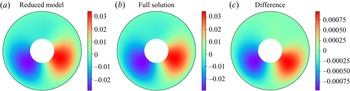
 $C_2$ model is in quantitative agreement with the full numerical simulation. This good agreement of the reduced model with full numerical simulations is also found for the concentration field, as shown in figure 3.
Comparison between the analytical prediction and the direct numerical simulation of the particle velocity and angular velocity in stationary, straight and circular phases. The system size is set to  $R=3.25$. The solid curves are obtained by a direct numerical solution of the
 $C_1$,
 $C_2$ equations. The symbols are the results of the full numerical simulations. In both cases the steady-state values are obtained by running the simulations for a long time until (of the order of
 $10^5a^2/D$). The horizontal axis is cut at
 $Pe=5.9$ above which the absolute value of the velocity does not seem to reach a steady state.

Comparison between the concentration fields  $c(\boldsymbol {r})-c_0(\boldsymbol {r})$ predicted by the reduced model and the direct numerical simulation. The system size is set to
 $R=3.25$. The Péclet number is set to
 $Pe=5.8$. Panel (a) shows the reduced model, (b) shows the full numerical simulation and (c) shows the difference. The coordinates are rotated to align the velocity with the horizontal axis in panels (a) and (b). The isotropic part of the concentration field
 $c_0(\boldsymbol {r})=\ln r/R$ is subtracted in panels (a) and (b) for better contrast..

The solution of the  $C_1$ and
 $C_2$ model shows that as the Péclet number is increased, the particle shows non-motile solution as the stable fixed point for
 $Pe< Pe_1$, straight motion (velocity is constant in time and finite, but angular velocity is equal to zero) for
 $Pe^*>Pe>Pe_1$, and a circular trajectory (both the swimming speed and the angular velocity remain fixed in time) for
 $Pe^{**}>Pe>Pe^*$. No stable fixed point solution could be obtained for
 $Pe>Pe^{**}$. Here we have
 $Pe^*\approx 5.77$ and
 $Pe^{**}\approx 5.9$. By increasing further
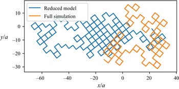
 $Pe$ we find that the solution becomes irregular, pointing to the occurrence of chaos (figure 4). This irregular mode is of peculiar nature, as demonstrated by the inspection of the time evolution of
 $C_1(t)$ and
 $C_2(t)$ in figure 5, made possible by the reduced model. The system possesses an unstable fixed point, corresponding to
 $C_1=0$ and
 $|C_2|=0.147$ for
 $Pe=5.95$. The phase of fixed-point value of
 $C_2$ is arbitrary due to the symmetry of the problem, which dictates that (8.1) remain invariant under transformation
 \begin{equation} C_1\rightarrow C1\, {\rm e}^{{\rm i}\phi_0}, \quad C_2\rightarrow C_2\, {\rm e}^{2{\rm i}\phi_0}, \end{equation}
corresponding to a rotation of the concentration field about the particle centre. Taking the fixed point  $C_2=0.147$, we observe that it is unstable with respect to the growth of
 ${\rm Re} C_1(t)$, although it is stable with respect to the growth of
 ${\rm Im} C_1(t)$. As
 $C_1(t)$ becomes large enough, the nonlinear effects lead to
 $C_2$ changing its sign, tending to the fixed point
 $C_2=-0.147$ (same absolute value as before but opposite sign). This fixed point is stable with respect to real perturbations of
 ${\rm Re} C_1$ but unstable with respect to perturbations of
 ${\rm Im} C_1$. This leads to a cyclic behaviour in which the changes of the sign of
 $C_2$ correspond to changes of
 $C_1$ between real and purely imaginary values. The explanation for this is that changing the sign of
 $C_2$ corresponds to a rotation of the second harmonic of the concentration field by an angle of
 $\pm {\rm \pi}/2$. From this, we conclude that the motion of the particle is divided between intervals of straight motion and intervals of quasistationary dynamics, during which the particle velocity makes a
 $90^\circ$ turn. Mathematically, this dynamics should correspond to a heteroclinic orbit, although the imperfection of the numerical solution and finite-precision arithmetic never allow us to reach this orbit. As a consequence we observe a chaotic random-walk dynamics, in which the left-hand or right-hand
 $90^\circ$ turns are probably determined by numerical noise. The circular trajectory and chaotic one have been also obtained by numerical simulation in Hu et al. (Reference Hu, Lin, Rafai and Misbah2019) using the full model. In a recent three-dimensional (3-D) simulation (Hu et al. Reference Hu, Lin, Rafai and Chaouqi2022) we have also reported on chaos via intermittency (exactly as in two dimensions). In another recent work (Misbah et al. Reference Misbah, Rizvi, Hu, Lin, Rafai and Farutin2021) by taking the set of (8.1) as a phenomenological model (extracted on the basis of symmetries, without reference to any given basic model) it has been shown that it reproduces a variety of solutions going from straight, circular to chaotic trajectories. The circular trajectory could even be obtained analytically (Misbah et al. Reference Misbah, Rizvi, Hu, Lin, Rafai and Farutin2021) from (8.1).
An irregular trajectory obtained from solution of (8.1) for  $Pe=5.95$.

Time-dependent dynamics of  $C_1(t)$ and
 $C_2(t)$ during the irregular motion. Panels (a) and (b) differ only by the range of the time axis. The simulations were started from an arbitrary initial conditions but a sufficient interval of transient dynamics is excluded from the image. The phases of
 $C_1(t)$ and
 $C_2(t)$ were then adjusted by an appropriate rotation of the concentration field in the
 $\phi$ domain, as given by (9.1a,b). The imaginary part of
 $C_2(t)$ is not shown because after the rotation it practically remains zero to machine precision after the initial transient is excluded..

10. Conclusion
We have extracted from a phoretic model in two dimensions, including advection and diffusion, a reduced model in terms of ordinary differential equations for the first two Fourier modes. This model captures, in a much less numerically expensive manner, essential features encountered in the full model. The derivation has been performed for the two first modes to cubic order. Extension to a higher number of modes can also be performed, as well as going to higher orders than cubic terms. This will be essential if one wishes to have a wider range of applicability of the method. The method is a priori valid close to critical point. Despite this restriction, the reduced model captures several essential features found in the full numerical simulation. The idea to focus on critical points is a classical method in nonlinear systems. Still, reducing the model to few harmonics has turned out to impressively capture nonlinear dynamics even very far from threshold. A prototypical example of these is the Rayleigh–Bénard convection (Dauby et al. Reference Dauby, Desaive, Bragard and Cerisier2001).
The derivation can be extended to three dimensions without any additional conceptual complication. The only modification is the use of spherical harmonics instead of Fourier modes. Note also that the full 3-D simulation (Hu et al. Reference Hu, Lin, Rafai and Chaouqi2022) has captured many of the features encountered in the full 2-D simulation (Hu et al. Reference Hu, Lin, Rafai and Misbah2019) (like meandering and transition to chaos via intermittency). The method has been exemplified here for a specific phoretic model. However, the same technique can be used for any swimmer powered by one or many chemical fields. Examples of great topicality are found in models of cell motility, involving acto-myosin kinetics inside the cell, outside and on the cell membrane, as well as cortex flow and flow in the suspending and internal fluids (Hawkins et al. Reference Hawkins, Poincloux, Bénichou, Piel, Chavrier and Voituriez2011; Callan-Jones et al. Reference Callan-Jones, Ruprecht, Wieser, Heisenberg and Voituriez2016; Farutin et al. Reference Farutin, Etienne, Misbah and Récho2019). Our general method did not have to specify explicitly the form of linear operator until § 7, precisely to highlight its generality.
In the specific phoretic model we considered here, it has been shown in three dimensions (Rednikov, Ryazantsev & Velarde Reference Rednikov, Ryazantsev and Velarde1994; Morozov & Michelin Reference Morozov and Michelin2019b) that the bifurcation from the non-motile to the motile state is not classical, in that  $\lvert V_0\rvert \sim (Pe-Pe_1)$, meaning that
 $V_0\sim \pm (Pe-Pe_1)$ (instead of
 $\pm (Pe-Pe_1)^{1/2}$). This is referred to as (Farutin & Misbah Reference Farutin and Misbah2021) a singular pitchfork bifurcation (it is not a transcritical bifurcation Morozov & Michelin (Reference Morozov and Michelin2019b)), owing to the appearance of an absolute value of
 $V_0$ (non-analytical form). However, we have shown recently (Farutin & Misbah Reference Farutin and Misbah2021) that the singular behaviour holds only for an infinite size. A finite size (even arbitrary large) removes the singularity and yields a classical pitchfork bifurcation. This has been demonstrated in our 3-D simulation (Hu et al. Reference Hu, Lin, Rafai and Chaouqi2022) where finite size leads to a pitchfork bifurcation. In the 2-D situation studied here, the finite size is already imperative due to the logarithmic behaviour with distance r of the concentration field of the non-motile solution; and leads again to a pitchfork bifurcation. The finite size is also natural in 2-D simulations (Hu et al. Reference Hu, Lin, Rafai and Misbah2019). In an extension to three dimensions one has to keep a finite size in order to allow for a regular expansion (in the way we did it here). However, there exist (Farutin & Misbah Reference Farutin and Misbah2021) other ways than resorting to finite size, in order to regularize the bifurcation. For instance, adding a linear consumption term in the diffusion equation removes the singularity both in two dimensions and three dimensions and leads to a classical pitchfork bifurcation (even for an infinite size). Studying steady motion along a straight line in an infinite 3-D domain without consumption is feasible (Rednikov et al. Reference Rednikov, Ryazantsev and Velarde1994) but the bifurcation turns out to be singular, so the situation is at present unclear for time-dependent solutions or solutions with curved trajectories.
Finally, since the reduced model equations have a form which depends only on symmetries, different models for active entities can be gathered together within a universal framework, so that they are all described by the same reduced evolution equations (of the type (8.1)). Differences between explicit models will be encoded only in the values of coefficients in the reduced model.
Funding
We thank CNES (Centre National d'Etudes Spatiales) for financial support and for having access to microgravity data, and the French–German university program ‘Living Fluids’ (grant CFDA-Q1-14) for financial support. W.-F.H. and T.-S.L. acknowledge the support by the National Center for Theoretical Sciences, Taiwan, and the National Science and Technology Council, Taiwan, under the research grant no. 111-2115-M-008-009-MY3 and no. 111-2628-M-A49-008-MY4, respectively.
Declaration of interests
The authors report no conflict of interest.
Appendix A. Inverting the diffusion operator
A solution to the equation
 \begin{equation} \frac{1}{r}\frac{{\rm d}}{{\rm d} r}\left(r\frac{{\rm d} F}{{\rm d} r}\right)- {\frac{l^2F}{r^2}}=G(r), \end{equation}
can be written as
 \begin{equation} F(r)= \begin{cases} \displaystyle \frac{1}{2l}\left[r^{{-}l}\int^r G(\rho)\rho^{1+l}\, {\rm d} \rho-r^l\int^r G(\rho)\rho^{1-l}\, {\rm d} \rho\right]+A_1 r^l+A_2r^{{-}l} & \textrm{for }l>0\\ \displaystyle \ln r\int^r G(\rho)\rho \, {\rm d} \rho-\int^r \rho\ln \rho G(\rho)d\rho+A_1+A_2\ln r & \textrm{for }l=0 \end{cases}, \end{equation}
where the constants  $A_1$ and
 $A_2$ are calculated by imposing the boundary conditions
 \begin{equation} \partial_rF(1)=0\quad F(R)=0. \end{equation}
The problem considered here requires solving (A1) with functions  $G(r)$ written as a combination of integer powers of
 $r$ and
 $\ln r$. This allows us to calculate the integrals in (A2) analytically.
Appendix B. Inverting the advection–diffusion operator
Suppose we have a system of equations
 \begin{equation} \left.\begin{array}{c@{}} \mu \boldsymbol f=(M+\boldsymbol u\otimes \boldsymbol v) \boldsymbol{\cdot} \boldsymbol x +\boldsymbol y\\ \langle \boldsymbol g,\boldsymbol x\rangle =0 \end{array}\right\}, \end{equation}
where  $\mu$ is a number,
 $M$ is a matrix,
 $\boldsymbol u,$
 $\boldsymbol v$,
 $\boldsymbol x$,
 $\boldsymbol y$,
 $\boldsymbol f$,
 $\boldsymbol g$ are vectors, and
 \begin{equation} \left.\begin{array}{c@{}} (M+\boldsymbol u\otimes \boldsymbol v)\boldsymbol{\cdot} \boldsymbol f=0,\\ \boldsymbol g\boldsymbol{\cdot} (M+\boldsymbol u\otimes \boldsymbol v)=0. \end{array}\right\} \end{equation}
The first (B1) corresponds to (5.10) where  $\mu$ represents
 $\partial _t C_l$,
 $M+\boldsymbol u\otimes \boldsymbol v$ is the linear operator
 $\hat L (Pe_l)$ (see (5.12)),
 ${\boldsymbol x}$ represents
 $\delta c_l$ and
 ${\boldsymbol y}$ represents
 $q_l$. The second equation represents the orthogonality condition (5.6). Equation (B2) represents the eigenvalue problem
 $\hat L (Pe_l) f_l (r)=0$ and its adjoint (5.3).
The goal of this appendix is to find the solution of the system (B1) representing  $\boldsymbol x$ and
 $\mu$ as a function of
 $M^{-1}$,
 $\boldsymbol u$,
 $\boldsymbol v$ and
 $\boldsymbol y$. First, we note the following relations:
 \begin{equation} \boldsymbol f\propto M^{{-}1}\boldsymbol{\cdot} \boldsymbol u,\quad \boldsymbol g\propto \boldsymbol v\boldsymbol{\cdot} M^{{-}1},\quad \langle \boldsymbol v,M^{{-}1}\boldsymbol{\cdot} \boldsymbol u\rangle={-}1, \end{equation}
which we obtain from (B2). Multiplying the first equation in (B1) by  $M^{-1}$, we get
 \begin{equation} \mu M^{{-}2}\boldsymbol{\cdot} \boldsymbol u=[I+(M^{{-}1}\boldsymbol{\cdot} \boldsymbol u)\otimes \boldsymbol v]\boldsymbol{\cdot} \boldsymbol x +M^{{-}1}\boldsymbol{\cdot} \boldsymbol y, \end{equation}
whence
 \begin{equation} \boldsymbol x=\mu M^{{-}2}\boldsymbol{\cdot} \boldsymbol u-(M^{{-}1}\boldsymbol{\cdot} \boldsymbol u)\langle \boldsymbol v,\boldsymbol x\rangle -M^{{-}1}\boldsymbol{\cdot} \boldsymbol y. \end{equation}
Equation (B5) implies the following ansatz for  $\boldsymbol x$:
 \begin{equation} \boldsymbol x={-}M^{{-}1}\boldsymbol{\cdot} \boldsymbol y+pM^{{-}1}\boldsymbol{\cdot} \boldsymbol u+qM^{{-}2}\boldsymbol{\cdot} \boldsymbol u, \end{equation}
where  $p$ and
 $q$ are two numbers to be determined. It is then straightforward to substitute equation (B6) into (B5) to get the values of
 $\mu$ and
 $q$ as
 \begin{equation} q=\mu=\frac{\langle \boldsymbol v,M^{{-}1}\boldsymbol{\cdot} \boldsymbol y\rangle}{\langle \boldsymbol v,M^{{-}2}\boldsymbol{\cdot} \boldsymbol u\rangle}. \end{equation}
The value of  $p$ is determined from the second equation of (B1). It is convenient that the solution (B7) use the vector
 $\boldsymbol v$ only as part of
 $\langle \boldsymbol v,\boldsymbol {\cdot }\rangle$ which allows us to use its definition
 $\langle \,\boldsymbol f,\boldsymbol v\rangle =Pef(1)$.
Appendix C. Coefficients of the reduced model
In the following we list the coefficients of the linear and quadratic terms and plot those of the cubic term:
 $$\begin{gather} \sigma_1=\frac{16
(Pe-Pe_{1}) (R^{2} \ln{(R)} - R^{2} + \ln{(R)} + 1)^{2}} {\begin{matrix}3
R^{6} + 8 R^{4} \ln{(R )}^{2} - 40 R^{4} \ln{(R )} + 19
R^{4} + 8 R^{2} \ln{(R)}^{2} + 4 R^{2} \ln{(R)}&\\ - 35 R^{2}
+ 12 \ln{(R)} + 13\end{matrix}}, \end{gather}$$
 $$\begin{gather}\alpha_1={-} \frac{
\begin{matrix}2 (R^{2} + 1 ) (20 R^{10} \ln{ (R )}^{2} - 40
R^{10} \ln{ (R )} + 21 R^{10} + 8 R^{8} \ln{ (R )}^{2} + 48
R^{8} \ln{ (R )} & \\ - 63 R^{8} + 16 R^{6} \ln{ (R )}^{3}
- 48 R^{6} \ln{ (R )}^{2} + 56 R^{6} \ln{ (R )} + 46 R^{6}
+ 32 R^{4} \ln{ (R )}^{3} & \\ - 56 R^{4} \ln{ (R )}^{2} -
8 R^{4} \ln{ (R )} + 6 R^{4} + 16 R^{2} \ln{ (R )}^{3} - 20
R^{2} \ln{ (R )}^{2}& \\ - 48 R^{2} \ln{ (R )} - 3 R^{2} - 8
\ln{ (R )} - 7 )\end{matrix}}{ \begin{matrix} R^{2} (R^{4}
+ 1 ) (R^{2} \ln{ (R )} - R^{2} + \ln{ (R )} + 1 ) (3 R^{6}
+ 8 R^{4} \ln{ (R )}^{2} - 40 R^{4} \ln{ (R )}& \\ +\, 19
R^{4} + 8 R^{2} \ln{ (R )}^{2} + 4 R^{2} \ln{ (R )} - 35
R^{2} + 12 \ln{ (R )} + 13 ) \end{matrix}},
\end{gather}$$
 $$\begin{gather}\sigma_2=\frac{3
(Pe-Pe_{2}) (R^{4} - 4 R^{2} + 4 \ln{(R )} + 3)^{2}}{\begin{matrix}12
R^{8} \ln{(R )} - 13 R^{8} + 16 R^{6} \ln{(R )} + 8 R^{6} +
12 R^{4} \ln{(R )} + 6 R^{4} - 8 R^{2}&\\ +\, 8 \ln{(R )} + 7\end{matrix}},
\end{gather}$$
 $$\begin{gather}\alpha_2=\frac{\begin{matrix} 3 (R^{4} + 1 )^{2} (R^{2} \ln{ (R )} - R^{2} + \ln{ (R )} + 1 ) (6 R^{6} \ln{ (R )} - 7 R^{6} + 6 R^{4} \ln{ (R )} & \\ +\, 9 R^{4} + 6 R^{2} \ln{ (R )} - 9 R^{2} + 6 \ln{ (R )} + 7 ) \end{matrix}} {\begin{matrix} (R^{2} + 1 )^{2} (R^{4} - 4 R^{2} + 4 \ln{ (R )} + 3 ) (12 R^{8} \ln{ (R )} & \\ - 13 R^{8} + 16 R^{6} \ln{ (R )} + 8 R^{6} + 12 R^{4} \ln{ (R )} + 6 R^{4} - 8 R^{2} + 8 \ln{ (R )} + 7 ) \end{matrix}}. \end{gather}$$
Appendix D. Explicit expression
Here we list the explicit expressions for  $\partial _t C_1$ and
 $\partial _t C_2$ for
 $R=3.25$. We first have simplified the expressions assuming
 $Pe$ to be close to the critical Péclet number
 $Pe_c=5.9561$, which is the critical Péclet number for
 $R=R_c=3.17493$, such that
 $Pe_1(R_c)=Pe_2(R_c)=Pe_c$. We then define
 $\Delta P=Pe-Pe_c=O(\epsilon )$ and truncate all expressions keeping only terms of order
 $O(\epsilon ^3)$ or higher, as follows:
 \begin{align} \partial_t C_1&= C_{1} (0.0484 + 0.1799 \Delta Pe- 0.00244 \Delta Pe^{2} )- C^{*}_{1} C_{2} ( 1.227+0.2467 \Delta Pe )\nonumber\\ &\quad - 0.2016 C_{1}|C_1|^2 - 3.077 C_{1} |C_2|^2 +O(\epsilon^4), \end{align}
 \begin{align} \partial_t C_2&=C_{2} (0.0411+ 0.3701 \Delta Pe- 0.00123 \Delta P\, {\rm e}^{2} )+C_{1}^{2} (0.5921+0.0905 \Delta Pe )\nonumber\\&\quad - 3.1214 |C_1|^2 C_{2} - 1.7893 |C_2|^2C_{2} {+O(\epsilon^4)}. \end{align}