







1. Introduction
Non-modal linear stability theory, based on solution of the initial-value problem in which the linearized Navier–Stokes equations can be recast, has elucidated laminar–turbulent transition paths in a number of shear flows in which linear modal theory, based on solution of the eigenvalue problem, has failed to predict transition (Trefethen et al. Reference Trefethen, Trefethen, Reddy and Driscoll1993; Schmid & Henningson Reference Schmid and Henningson1994; Tumin & Reshotko Reference Tumin and Reshotko2001; Tempelmann, Hanifi & Henningson Reference Tempelmann, Hanifi and Henningson2010). To date, the majority of transient growth studies have been performed in a local incompressible analysis framework, considering flows a basic state that is homogeneous in two spatial directions; Schmid & Henningson (Reference Schmid and Henningson2001) and Schmid (Reference Schmid2007) provide extensive reviews of early work in this steadily growing field. Comparatively less transient growth analyses have addressed compressible flow, the first such effort being the work of Hanifi, Schmid & Henningson (Reference Hanifi, Schmid and Henningson1996), who demonstrated the potential of the flat plate boundary layer to sustain algebraic energy growth of streamwise-aligned perturbations at conditions subcritical to exponential amplification of Tollmien–Schlichting or crossflow disturbances. More recently, Tumin & Reshotko (Reference Tumin and Reshotko2003) relaxed the parallel flow assumption and found that the optimal disturbances also correspond to steady counter-rotating streamwise vortices. Zuccher, Tumin & Reshotko (Reference Zuccher, Tumin and Reshotko2006) and Zuccher et al. (Reference Zuccher, Shalaev, Tumin and Reshotko2007) analysed the flow past a sphere and a sharp cone, and found that flow divergence has significant effects on the transient growth phenomenon. Moreover, Tempelmann, Hanifi & Henningson (Reference Tempelmann, Hanifi and Henningson2012) investigated the importance of the transient growth in crossflow-dominated three-dimensional compressible boundary layers.
In the framework of global linear stability theory (Theofilis Reference Theofilis2011), transient growth analyses have also commenced in the incompressible limit and demonstrated the potential of laminar flow separation to sustain levels of algebraic energy growth sufficiently high to bypass the linear modal instability laminar–turbulent transition scenario (Sherwin & Blackburn Reference Sherwin and Blackburn2005; Blackburn, Barkley & Sherwin Reference Blackburn, Barkley and Sherwin2008). In the wake of the circular cylinder (Abdessemed et al. Reference Abdessemed, Sharma, Sherwin and Theofilis2009a), in a cascade of low-pressure turbine blades (Abdessemed, Sherwin & Theofilis Reference Abdessemed, Sherwin and Theofilis2009b; Sharma et al. Reference Sharma, Abdessemed, Sherwin and Theofilis2011) and in massively separated flow over stalled aerofoils (He et al. Reference He, Gioria, Pérez and Theofilis2017), the three-dimensional stationary global eigenmode discovered by Theofilis, Hein & Dallmann (Reference Theofilis, Hein and Dallmann2000) to underpin self-excitation of steady nominally two-dimensional laminar separation bubbles has been identified to co-exist with the well-known amplified Kelvin–Helmholtz eigenmode that develops at the shear layer of a laminar separation bubble (Dovgal, Kozlov & Michalke Reference Dovgal, Kozlov and Michalke1994). It was further shown that linear optimal disturbances in all of these flows evolve into travelling Kelvin–Helmholtz instabilities in the limit of an asymptotically large time horizon, thus providing a physical link between results of the initial-value and eigenvalue problems. Paredes, Choudhari & Li (Reference Paredes, Choudhari and Li2017, Reference Paredes, Choudhari and Li2018), in their study of the blunt-body paradox associated with leeward transition over a hypersonic spherical forebody, have discussed the important effect of the choice of an appropriate energy norm in their analysis, and highlighted the need to investigate further the optimal-growth criterion underlying the Reshotko & Tumin (Reference Reshotko and Tumin2004) correlation.
Flow over an elliptic cone studied herein arises from the HIFiRE hypersonic flight test programme, led by the Air Force Research Laboratory and the Australian Defence Science and Technology Organization (Dolvin Reference Dolvin2008). The aim of this effort has been to demonstrate technologies that are critical to the design of next-generation hypersonic aerospace systems, including boundary layer laminar–turbulent transition, prediction and control. The first configuration in the programme, HIFiRE-1, used a 7 $^\circ$ half-angle cone to obtain in-flight transitional and turbulent boundary layer heating data on axisymmetric configurations. The design of this experiment, the associated pre-flight effort and actual flight data, as well as transitional analysis, have been discussed in detail in Kimmel et al. (Reference Kimmel, Adamczak, Gaitonde, Rougeux and Hayes2007, Reference Kimmel, Adamczak, Paull, Paull, Shannon, Pietsch, Frost and Alesi2011), Kimmel (Reference Kimmel2008), Adamczak et al. (Reference Adamczak, Kimmel, Paull and Alesi2011), Stanfield, Kimmel & Adamczak (Reference Stanfield, Kimmel and Adamczak2012) and Li et al. (Reference Li, Choudhari, Chang, Kimmel, Adamczak and Smith2011), further elaborating on the overview of earlier transition research on circular base cones (Schneider Reference Schneider2004).
On the other hand, another configuration in the program, HIFiRE-5, was designed specifically to provide transition data in an essentially three-dimensional boundary layer. This platform consists of a blunt-nosed elliptic cone of 2 : 1 aspect ratio and 0.86 m in length, mounted on an Orion booster (Kimmel et al. Reference Kimmel, Adamczak, Berger and Choudhari2010). The specific aspect ratio was chosen since it presents significant crossflow and second-mode instabilities that are expected to be the dominant instability mechanisms in three-dimensional boundary layers at hypersonic speeds. The minor axis of the cross-section is defined as the centreline, while the major axis is referred to as the attachment line. The blunted tip consists of a 2.5 mm radius circular arc that is tangent to the cone rays inscribed in the minor axis, while it retains a 2 : 1 elliptical cross-section to the tip.
Several efforts spanning two decades have contributed to understanding hypersonic transition on elliptic cones. From an experimental point of view, Holden (Reference Holden1998) obtained schlieren images of hypersonic flow over a 4 : 1 aspect ratio elliptic cone at angles of attack from  $0^\circ$ to
 $5^\circ$, and reported that the transition front moves towards the base of the cone with increasing angle of attack. Schmisseur, Schneider & Collicott (Reference Schmisseur, Schneider and Collicott1998, Reference Schmisseur, Schneider and Collicott1999) measured the boundary layer response to a laser-generated localized free stream disturbance on the same 4 : 1 aspect ratio elliptic cone in a Mach 4 quiet tunnel at unit Reynolds number
 $4.5 \times 10^6$ m
 $^{-1}$. At these conditions, the undisturbed flow field was shown to be practically laminar in its entirety. The surface measurements also indicated that the boundary layer response to disturbance is concentrated near the centreline. Kimmel, Poggie & Schwoerke (Reference Kimmel, Poggie and Schwoerke1999) investigated the influence of base laminar crossflow on transition in the hypersonic boundary layer over a sharp-nosed 2 : 1 aspect ratio elliptic cone employing schlieren imaging and surface oil flow visualization. Unlike hypersonic flow over planar and axisymmetric bodies, the transition front was found not to be driven by second mode instability. They found that the transition front was non-uniform, with the earliest signs of boundary layer transition being recorded in the vicinity of the centreline. Huntley & Smits (Reference Huntley and Smits2000) studied in detail centreline boundary layer transition on a sharp-nosed 4 : 1 aspect ratio elliptic cone at Mach number 8 using CO
 $_2$-enhanced filtered Rayleigh scattering. In line with the results of Kimmel et al. (Reference Kimmel, Poggie and Schwoerke1999), and despite the different cone aspect ratio, these authors also found transition to occur in the vicinity of the centreline, and presented for the first time detailed results of the early stages of transition in this region. Juliano & Schneider (Reference Juliano and Schneider2010) performed experiments in the Boeing/AFOSR Mach-6 Quiet Tunnel (BAM6QT) facility with an aspect ratio 2 elliptic cone, and showed that the dominant mechanisms leading to transition are streamwise-aligned structures, identified as crossflow vortices between the centreline and the attachment line region. In the experiments of Borg, Kimmel & Stanfield (Reference Borg, Kimmel and Stanfield2012), it was found that selective choice of spacing between roughness elements introduced can excite wavelengths that would have been stable in the unperturbed boundary layer. Heat flux and boundary layer transition were measured by Juliano, Borg & Schneider (Reference Juliano, Borg and Schneider2015) in the BAM6QT facility, where two different transitional modes were found, the first along the centreline and the second at the crossflow region. Moreover, these authors showed that both transitional modes were delayed when tunnel noise level was reduced, and conversely, the transition front moved forward when altitude was increased. Flight testing of the HIFiRE-5 commenced in 2012, although in that first flight the highest Mach number achieved in flight was 3 instead of the targeted 7 (Kimmel et al. Reference Kimmel, Adamczak, Juliano and Paull2013). Analysis of the flight data obtained revealed a transition pattern consistent with previous numerical and experimental studies, namely the presence of early transition at the centreline of the vehicle. Subsequently, Juliano, Adamczak & Kimmel (Reference Juliano, Adamczak and Kimmel2014) performed a full analysis of the flight data during the supersonic descent phase, and reported two distinct boundary layer transition mechanisms: the first caused transition at the centreline, while the second was related to transition at the leading edge and grows rapidly over a small range of free stream unit Reynolds numbers. The second flight test, called HIFiRE-5b, was performed in 2016 and was fully successful, reaching its target Mach number
 $7.5$ and apogee
 $\sim$300 km; details and analysis of the flight can be found in Kimmel et al. (Reference Kimmel, Adamczak, Hartley, Alesi, Frost, Pietsch, Shannon and Silvester2017, Reference Kimmel, Adamczak, Hartley, Alesi, Frost, Pietsch, Shannon and Silvester2018) and Borg & Kimmel (Reference Borg and Kimmel2018).
From a theoretical point of view, early work employing the parabolized Navier–Stokes equation was performed by Lyttle & Reed (Reference Lyttle and Reed1995), who analysed flow on an elliptic cone at zero angle of attack and different cross-sections, and reported the existence of crossflow for all geometries investigated, but no crossflow transition in the range of parameters examined. The first inviscid linear global instability analysis was performed by Theofilis (Reference Theofilis2000, Reference Theofilis2002), who addressed supersonic and hypersonic flow over elliptic cones of different aspect ratios by solving the two-dimensional Rayleigh equation on a body-fitted coordinate system, and discovered distinct families of hydrodynamic and acoustic instabilities. Choudhari et al. (Reference Choudhari, Chang, Jentink, Li, Berger, Candler and Kimmel2009) solved the corresponding two-dimensional viscous eigenvalue problem on a rectangle containing the main basic flow features around the centreline, for in-flight and wind tunnel conditions. The steady laminar three-dimensional base flows were calculated using a variety of structured and unstructured codes (Cheatwood & Gnoffo Reference Cheatwood and Gnoffo1996; Nompelis, Drayna & Candler Reference Nompelis, Drayna and Candler2005; Baurle et al. Reference Baurle, White, Drozda and Norris2020), while the main result of the eigenvalue problem solution was identification of unstable centreline global modes at all flow conditions examined. Paredes & Theofilis (Reference Paredes and Theofilis2015) and Paredes et al. (Reference Paredes, Gosse, Theofilis and Kimmel2016) also solved the two-dimensional eigenvalue problem on a body-fitted elliptic coordinate system that extended from the centreline to the attachment line of an elliptic cone at zero angle of attack. They interrogated flow instability at 21.8 km and 33 km altitudes, at Mach numbers 7.45 and 7, and unit Reynolds numbers  $1.015 \times 10^7$ m
 $^{-1}$ and
 $1.89 \times 10^6$ m
 $^{-1}$, respectively. They reported the existence of four classes of linear modal disturbances: symmetric and antisymmetric centreline instabilities associated with the shear layer formed due to the lift-up effect at the centreline region, as seen in the analysis of Choudhari et al. (Reference Choudhari, Chang, Jentink, Li, Berger, Candler and Kimmel2009), alongside high-frequency attachment line modes, oblique second (Mack) modes and crossflow instabilities in the boundary layer between the centreline and attachment line. Large-scale numerical simulation of the HIFiRE-5 elliptic cone model was performed by Dinzl & Candler (Reference Dinzl and Candler2017) at the conditions of the Borg et al. (Reference Borg, Kimmel and Stanfield2012) experiment. These authors reported a Reynolds number dependence in the dominant stationary crossflow wavelength, with higher Reynolds numbers supporting instabilities corresponding to smaller wavelengths. Furthermore, streamwise-aligned structures were identified as streaks in agreement with experimental results, and the formation of streamwise-aligned structures was attributed to the strong interaction between the streamwise velocity and the wall. On the other hand, Moyes et al. (Reference Moyes, Kocian, Mullen and Reed2018) employed nonlinear parabolized stability equations (PSE) and linear spatial (modal) two-dimensional instability analysis, and demonstrated that coupling nonlinear PSE and global linear instability equations can provide a framework capable of predicting transition onset in flows with stationary crossflow as the dominant mechanism. Tufts et al. (Reference Tufts, Borg, Gosse and Kimmel2018a) summarized work performed up to that point, and discussed the strengths and weaknesses of using computation, ground tests and flight tests to predict laminar–turbulent transition over the HIFiRE-5 elliptic cone geometry. Very recently, Shi, Zhu & Lee (Reference Shi, Zhu and Lee2020) developed an engineering model for transition prediction, based on new wind-tunnel experiments and flight data correlations. The proposed model is shown to agree well with the HIFiRE-5b flight data and with Purdue University wind tunnel test data (Juliano & Schneider Reference Juliano and Schneider2010). However, in the crossflow region closer to the centreline, disagreements were observed between the experimental results of these authors when compared with flight testing data. Since classical linear stability analysis (Paredes et al. Reference Paredes, Gosse, Theofilis and Kimmel2016; Moyes et al. Reference Moyes, Kocian, Mullen and Reed2018) predicts slow growth of disturbances in that region, no explanation of these differences could be provided on the basis of linear modal analysis. Finally, Choudhari, Li & Paredes (Reference Choudhari, Li and Paredes2020) extended the analysis of the HIFiRE-5b flight experiment using local theory (Tufts, Gosse & Kimmel Reference Tufts, Gosse and Kimmel2018b) to study the linear stability of the boundary layer flow near the centreline of the elliptic cone, and found an
 $N$-factor that peaks close to the value that correlates with Mack mode transition in the HIFiRE-1 circular cone experiment.
The present work aims to fill the knowledge gap regarding linear non-modal instability on an aspect ratio 2 elliptic cone, and complements earlier modal analysis of the same problem discussed by Paredes & Theofilis (Reference Paredes and Theofilis2015) and Paredes et al. (Reference Paredes, Gosse, Theofilis and Kimmel2016). The base flow model and analysis parameters used are unit Reynolds numbers  $Re'= 1.89 \times 10^{-6}$ and
 $1.07 \times 10^{-7}$ m
 $^{-1}$, at Mach numbers
 $Ma = 8.05$ and
 $7.45$, corresponding to altitudes between the highest,
 $33$ km, and the lowest,
 $21$ km, in cruise flight at zero angle of attack. By contrast to Paredes et al. (Reference Paredes, Gosse, Theofilis and Kimmel2016), the initial-value problem is solved over time horizons sufficiently long for the modal analysis results to be recovered, and the magnitude of transient energy growth is documented. Some guidance for the choice of parameters in the present transient growth analysis has been provided by the local analysis results of Quintanilha et al. (Reference Quintanilha, Belesiotis, Theofilis and Hanifi2018), who addressed the potential of one-dimensional base flow profiles, at various streamwise stations and all azimuthal locations, from the centreline to the attachment line, to sustain transient growth. The present work constructs the firm theoretical foundation for two-dimensional transient growth to be performed on the geometry at hand, thus relaxing the approximation of azimuthal base flow homogeneity used by Quintanilha et al. (Reference Quintanilha, Belesiotis, Theofilis and Hanifi2018).
The theoretical framework to perform non-modal linear instability analysis on arbitrary two-dimensional compressible flows with two inhomogeneous spatial directions is introduced in § 2. The coordinate transformation to apply the theory to the elliptic cone problem at hand, as well as the numerical implementation of the non-modal analysis framework in the massively parallel global instability analysis code LiGHT, are discussed in § 3; validations of the code are presented in § 4.2. The main body of results obtained is shown in §§ 4.3.1 and 4.3.2, respectively discussing one- and two-dimensional theory results on linear optimal initial conditions, optimal perturbations at conditions of maximal transient energy growth and the asymptotic behaviour of transient linear perturbations in the large time horizon limit. In addition, comparison of the transient growth results with experimental flow visualization is addressed. A summary of the findings and conclusions is furnished in § 5.
2. Non-modal linear stability theory
The present work addresses linear instability on the aspect ratio 2 elliptic cone model of the HIFiRE-5 test geometry from the point of view of numerical solution of the initial-value problem (IVP) in which the linearized Navier–Stokes equations (LNSE) may be recast. Results of the eigenvalue problem (EVP) solved by Paredes et al. (Reference Paredes, Gosse, Theofilis and Kimmel2016) are recovered in the limit of large time horizons and serve to validate the present time-dependent analysis methodology; key theoretical points are discussed next.
2.1. The initial-value problem
Any unsteady three-dimensional flow quantity  ${\boldsymbol q}({\boldsymbol x},t)= (u, v, w, T, p)^{\rm T}({\boldsymbol x},t)$ is decomposed into a steady laminar base flow
 ${\bar {\boldsymbol {q}}}({\boldsymbol {x}})$, upon which an unsteady small-amplitude disturbance,
 ${\tilde {\boldsymbol {q}}}({\boldsymbol {x}},t)$, is superposed, i.e.
 \begin{equation} {\boldsymbol{q}}({\boldsymbol{x}},t) = {\bar{\boldsymbol{q}}}({\boldsymbol{x}}) + \epsilon\, {\tilde{\boldsymbol{q}}}({\boldsymbol{x}},t), \quad {\rm with} \ \epsilon \ll 1, \end{equation}
where  $\boldsymbol {x} = (\xi,\eta,\zeta )$ gives the three spatial directions in a curvilinear coordinate system. Substituting this decomposition into the dimensionless compressible Navier–Stokes equations gives rise to the LNSE (e.g. Hanifi et al. Reference Hanifi, Schmid and Henningson1996; Choudhari et al. Reference Choudhari, Chang, Jentink, Li, Berger, Candler and Kimmel2009; Paredes et al. Reference Paredes, Gosse, Theofilis and Kimmel2016). These equations can be written as an IVP in the form
 \begin{equation} \frac{\partial\tilde{\boldsymbol{q}}}{\partial t} = \mathcal{L}{\tilde{\boldsymbol{q}}} , \end{equation}
where  ${\tilde {\boldsymbol {q}}}(\xi,\eta,\zeta,t) = (\tilde {u}, \tilde {v}, \tilde {w}, \tilde {T}, \tilde {P})^{\rm T}$ is the vector containing the disturbance functions of velocity, temperature and pressure, and
 $\mathcal {L}$ contains the base flow, its spatial derivatives and the Reynolds (
 $Re$) and Mach (
 $Ma$) numbers as control parameters.
The exact solution of the IVP is written with the aid of the matrix exponential (Moller & van Loan Reference Moller and van Loan1978, Reference Moller and van Loan2003):
 \begin{equation} \hat{\boldsymbol q}(t)=\hat{\boldsymbol q}(0) \, {\rm e}^{{\mathcal{L}}t}. \end{equation}
If this matrix were normal, then its eigenvalue spectrum could be used to simplify this expression. However,  $\mathcal {L}$ of the LNSE is (highly) non-normal leading to a non-trivial behaviour at early times, which arises on account of the near-parallel nature of certain eigenvectors (Schmid & Henningson Reference Schmid and Henningson2001) in the eigenspectra.
2.2. Quantitative description of transient energy growth
Linear non-modal instability is defined through algebraic growth or decay of disturbance energy, scaled to unity at time  $t=0$, over a prescribed time interval
 $0\le t\le \tau$ (Luchini Reference Luchini1996; Corbett & Bottaro Reference Corbett and Bottaro2001; Schmid & Henningson Reference Schmid and Henningson2001; Schmid Reference Schmid2007; Luchini & Bottaro Reference Luchini and Bottaro2014). Optimizing algebraic growth within a given time horizon,
 $\tau$, over all permissible initial conditions permits us to define a quantitative measure of transient energy growth through the gain function
 $G(\tau )$, defined as the maximum energy amplification:
 \begin{equation} G(\tau) = \max_{{\tilde{\boldsymbol{q}_0}}} \frac{E({\tilde{\boldsymbol{q}}}(\tau))}{E({\tilde{\boldsymbol{q}}_0})}, \end{equation}
where  $E(\tilde {\boldsymbol {q}(\tau )}$) is the energy of the disturbance at a given time,
 $\tau$, the latter being a parameter in the analysis. Substituting (2.3) into the above definition of energy amplification gives
 \begin{equation} G(\tau) =\max_{{\tilde{\boldsymbol{q}_0}}} \frac{\|{\tilde{\boldsymbol{q}}}(\tau)\|^{2}_{E}}{\|{\tilde{\boldsymbol{q}}_{0}}\|^{2}_{E}} =\max_{{\tilde{\boldsymbol{q}_0}}} \frac{\|{\exp(\tau \mathcal{L} {\tilde{\boldsymbol{q}}_0})} \|^{2}_{E}}{\|{\tilde{\boldsymbol{q}}_0}\|^{2}_{E}} =\|{\exp(\tau \mathcal{L})}\|^{2}_{E}. \end{equation}
The norm of the matrix exponential represents the largest amplification of energy that any infinitesimal initial disturbance can experience within a given time interval, and will be defined shortly.
As discussed by Moller & van Loan (Reference Moller and van Loan1978), irrespective of the spatial discretization approach employed, the large condition number of the matrix discretizing the linear operator makes exact computation of the matrix exponential challenging. Here, an eigenvalue decomposition of the numerical linear operator  $\mathcal {L}$ is used to approximate the matrix exponential by
 \begin{equation} \|{\exp(\tau \mathcal{L})}\|^{2}_{E} =\|{\exp(\tau \mathcal{V} \varLambda \mathcal{V}^{{-}1})}\|^{2}_{E} =\| \mathcal{V} \exp(\tau \varLambda) \mathcal{V}^{{-}1}\|^{2}_{E}, \end{equation}
where  $\varLambda$ and
 $\mathcal {V}$ are matrices containing the eigenvalues and the corresponding normalized eigenvectors of
 $\mathcal {L}$, respectively. Note that up to this point, no approximations regarding the shape of the disturbances or their temporal behaviour have been introduced. While the formalism is identical in both one- and two-dimensional non-modal analysis, calculation of the matrix exponential in the present analysis context has required inclusion of a rather large number of eigenmodes, as will be seen in § 4.2.
2.3. Definition of the energy norm
Equation (2.4) requires the definition of an inner product and its associated norm. These quantities constitute the fundamental measure of time-dependent transient perturbation behaviour. Mathematically, the inner product and an associated norm can be written as
 \begin{equation} \langle{\tilde{\boldsymbol{q}}}_i,{\tilde{\boldsymbol{q}}}_j \rangle = \int^{\infty}_{0} \int^{\infty}_{0} {\tilde{\boldsymbol{q}}}_i^H \mathcal{M} {\tilde{\boldsymbol{q}}}_j J \, {\rm d}\eta \, {\rm d}\zeta, \quad 2E = \langle{\tilde{\boldsymbol{q}}},{\tilde{\boldsymbol{q}}}\rangle = \|{\tilde{\boldsymbol{q}}}\|^2_E, \end{equation}
where  $J$ is the Jacobian of the coordinate transformation. As pointed out by Hanifi et al. (Reference Hanifi, Schmid and Henningson1996), the energy density of a disturbance is a natural and physically meaningful measure of its size in the context of an incompressible flow. However, no obvious choice exists when dealing with compressible flows. Chu (Reference Chu1965) provided a discussion of this energy norm and the possibility of using different
 $\tilde {\boldsymbol {q}}$ vectors to approximate it, while Hanifi et al. (Reference Hanifi, Schmid and Henningson1996) re-derived in a non-modal analysis context the compressible energy norm proposed by Mack (Reference Mack1969) in the context of modal linear instability, requiring pressure work to be conservative. The energy norm definition proposed by Hanifi et al. (Reference Hanifi, Schmid and Henningson1996) can be adapted to our
 $\tilde {\boldsymbol {q}}$ vector using the ideal gas law
 \begin{equation} \mathcal{M}={\rm diag} \left(\bar{\rho}, \bar{\rho}, \bar{\rho}, \frac{\bar{\rho}}{\bar{T}} \left( \frac{1}{\gamma (\gamma - 1) M^2} - 1 \right), \frac{1}{\bar{\rho} \gamma M^2}\right), \end{equation}
and will be used in the present analysis. In one-dimensional transient growth analysis, the base flow quantities and amplitude functions are taken as one-dimensional functions of the wall-normal spatial coordinate. In the two-dimensional analysis, they are taken as functions of the plane on which the EVP is solved; the latter is discussed in some detail next.
2.4. Computation of transient energy growth
In order to address non-modal linear one- and two-dimensional instability on the elliptic cone, the linearized governing equations (2.2) are written for an expansion of the vector quantities  $\tilde {\boldsymbol {q}}$ that is inhomogeneous in the spanwise,
 $\zeta$, and wall-normal,
 $\eta$, spatial directions, while it is treated as homogeneous along the streamwise,
 $\xi$, spatial direction. Explicitly, the ansatz employed is
 \begin{equation}
{\tilde{\boldsymbol{q}}}(\xi,\eta,\zeta,t) =
{\hat{\boldsymbol{q}}}(\eta,\zeta) \, {\rm
e}^{{\rm i}(\alpha \xi -
\omega t)}, \end{equation}
where  $\alpha$ is a real wavenumber along the
 $\xi$ direction, associated with a streamwise periodicity length
 $L_\xi ={2{\rm \pi} }/{\alpha }$. In a temporal analysis framework,
 $\omega$ is a complex eigenvalue, where the flow is classified as linearly unstable if the imaginary part of one or more values of
 $\omega$ is positive. Substituting (2.9) into (2.2) results in the following complex non-symmetric generalized EVP
 \begin{equation} \mathcal{A} {\hat{\boldsymbol{q}}} = \omega \mathcal{B} \hat{\boldsymbol{q}}, \end{equation}
where the operators  $\mathcal {A}$ and
 $\mathcal {B}$ can be written explicitly to give
 \begin{equation} \left( {\mathsf{A}}^i_j\,\frac{\partial^2}{\partial\eta^2} + {\mathsf{B}}^i_j\,\frac{\partial^2}{\partial\zeta^2} + {\mathsf{C}}^i_j\, \frac{\partial^2}{\partial\eta\,\partial \zeta} + {\mathsf{D}}^i_j\,\frac{\partial}{\partial\eta} + {\mathsf{E}}^i_j\, \frac{\partial}{\partial\zeta} + {\mathsf{F}}^i_j \right) \hat{q}_j = \omega {\mathsf{G}}^i_j \hat{q}_j. \end{equation}
Here,  $\boldsymbol{\mathsf{A}},\boldsymbol{\mathsf{B}},\boldsymbol{\mathsf{C}},\boldsymbol{\mathsf{D}},\boldsymbol{\mathsf{E}},\boldsymbol{\mathsf{F}} \text{ and }\boldsymbol{\mathsf{G}}$ are
 $5\times 5$ matrices, and the superscript
 $i = (1,2,3,4,5)$ corresponds to the linearized equations of motion,
 $1$ referring to the momentum equation in
 $\xi$,
 $2$ to the momentum equation in
 $\eta$,
 $3$ to the momentum equation in
 $\zeta$,
 $4$ to the energy, and
 $5$ to the continuity equation. The subscript
 $j = (1,2,3,4,5)\equiv (\hat {u},\hat {v},\hat {w},\hat {T},\hat {p})$ corresponds to the five disturbances variables. The non-zero elements can be found in Paredes (Reference Paredes2014) and Quintanilha (Reference Quintanilha2021). It is also noted that the linear operator
 $\mathcal {L}$ defined in (2.2) is a shorthand notation for
 \begin{equation} \mathcal{L}=\mathcal{B}^{{-}1}\mathcal{A}. \end{equation}
Equation (2.11) is the tensor form of the global linear stability equations in a generalized frame of reference. As shown in a number of studies in the incompressible limit (e.g. Alizard & Robinet Reference Alizard and Robinet2007; Theofilis Reference Theofilis2017), the global linear stability equations and the linear PSE lead to identical results when initialized with consistent inflow boundary conditions for the flow perturbations.
In direct analogy to the analysis of Hanifi et al. (Reference Hanifi, Schmid and Henningson1996), we restrict attention to the space spanned by the first  $N$ (non-orthogonal) eigenfunctions of (2.10) and express the state vector
 $\tilde {\boldsymbol {q}}$ in terms of the basis
 \begin{equation} {\tilde{\boldsymbol{q}}} = \sum_{k=1}^{N} \mathcal{K}_k(\tau)\,{\hat{\boldsymbol{q}}}_k, \end{equation}
where
 \begin{equation} \mathcal{K}_k(\tau) = \mathcal{K}_k (0) \exp(-{{\rm i}} \omega_k \tau) \end{equation}
are time-dependent expansion coefficients. Thus the eigenvalues represent the linear evolution operator projected onto the space spanned by the first  ${N}$ eigenvectors. Restricting the transient growth analysis to this space and applying the scalar product and the energy norm defined previously, leads to
 \begin{equation} G(\tau) = G(\alpha,Re,M,\tau) = \max_{{\tilde{\boldsymbol{q}}}_0} \frac{\| {\tilde{\boldsymbol{q}}}(\tau) \|^2_E}{\| {\tilde{\boldsymbol{q}}}(0) \|^2_E} = \| {\exp (-{{\rm i}} \tau \mathcal{B}^{{-}1} \mathcal{A})}\|^{2}_E = \| F \varLambda F^{{-}1} \|^2_2, \end{equation}
where
 \begin{equation} \varLambda = {\rm diag} ( \exp(- {{\rm i}} \tau \omega_1) , \exp(- {{\rm i}} \tau \omega_2),\ldots, \exp(- {{\rm i}} \tau \omega_N)), \quad \mathcal{F} = F^H F, \end{equation}
and  ${\mathcal {F}_{ij}}$ is defined as the scalar product presented in (2.7a,b). The maximum gain is thus obtained as the square of the largest singular value (e.g. Taira et al. Reference Taira, Brunton, Dawson, Rowley, Colonius, McKeon, Schmidt, Gordeyev, Theofilis and Ukeiley2017).
2.5. Computation of linear optimal disturbances
In non-normal systems exhibiting algebraic energy growth, it is interesting to compute the initial condition that maximizes energy amplification at early times,  $G_{opt}\equiv G(\tau _{opt})$. This initial condition can be different for different times, and the resulting curve
 $G(t)$ can be seen as the envelope of the energy evolution of individual initial conditions. In order to determine the initial condition that leads to maximum amplification at a given time,
 $\tau _{opt}$, a singular value decomposition (SVD) of the expression in (2.15) can be performed:
 \begin{equation} \mathcal{C} V = U \varSigma, \end{equation}
where  $\mathcal {C} = F \varLambda F^{-1}$,
 $\boldsymbol{\mathsf{V}}$ and
 $\boldsymbol{\mathsf{U}}$ are unitary matrices with orthonormalized columns, and
 $\varSigma$ is a diagonal matrix consisting of the singular values ordered in size, i.e.
 $\sigma _1 \ge \sigma _2 \ge \cdots \ge \sigma _N$. The dominant singular value is equivalent to the energy norm of
 $\exp (-\tau \omega _k)$. Thus extracting the principal column vectors of
 $\boldsymbol{\mathsf{V}}$ and
 $\boldsymbol{\mathsf{U}}$ leads to
 \begin{equation} \mathcal{C} \boldsymbol{v}_1 = \sigma_1 \boldsymbol{u}_1. \end{equation}
As pointed out by Schmid & Henningson (Reference Schmid and Henningson1994), this equation can be interpreted as a mapping  $\mathcal {C}$ of an input vector
 $\boldsymbol{v}_1$ onto an output vector
 $\boldsymbol{u}_1$ stretched by a factor of the largest singular value; see also the related discussion by Taira et al. (Reference Taira, Brunton, Dawson, Rowley, Colonius, McKeon, Schmidt, Gordeyev, Theofilis and Ukeiley2017). Therefore, the optimal initial condition can be obtained from the principal right singular value vector. Finally, to recover the initial expansion coefficients of (2.13), which give the optimal disturbances associated with a particular amplification, it is necessary to write
 $\boldsymbol{v}_1$ in the basis
 $\{ {\hat {\boldsymbol {q}}}_1,\ldots, {\hat {\boldsymbol {q}}}_N\}$ as
 \begin{equation} \boldsymbol{v}_1 = F \mathcal{K}_0. \end{equation}
In summary, the computational steps required to recover the optimal initial condition are an SVD of the matrix exponential evaluated at different times  $\tau$. Following closely the nomenclature adopted by Hanifi et al. (Reference Hanifi, Schmid and Henningson1996), two different symbols will be used in the following discussion. We use
 \begin{equation} G_{max} = \max [ G(t \ge 0)] \end{equation}
to define the maximum value obtained by  $G(t)$ over the whole time interval. A formula for approximating this value will be discussed later when comparing the EVP and IVP solutions. For this case,
 $t_{max}$ can be defined as the time at which this maximum is achieved. However, if we consider only the initial short time before the modal growth takes place, then we can define the optimal initial growth as
 \begin{equation} G_{opt} = G(\tau=\tau_{opt}), \end{equation}
where  $\tau _{opt}$ is the time at which the largest transient growth is obtained.
3. Numerical implementation
The transformation of the physical  $(x,y,z)$ to the computational
 $(\xi, \eta, \zeta )$ coordinate system is performed using the elliptic confocal transformation discussed by Theofilis (Reference Theofilis2000) and Paredes et al. (Reference Paredes, Gosse, Theofilis and Kimmel2016):
 \begin{equation} x = \xi, \quad y = c \xi \sinh (\eta_0 + \eta) \sin \zeta, \quad z = c \xi \cosh (\eta_0 + \eta) \cos \zeta, \end{equation}
where  $c$ sets the half-angle of the cone minor axis,
 $\theta = 7^{\circ }$, via
 \begin{equation} c =\frac{\tan\theta }{\sinh \eta_0 }, \end{equation}
and
 \begin{equation} \eta_0 = \tanh^{{-}1} \frac{1}{AR}, \end{equation}
is a parameter controlling the aspect ratio ( $AR$) of the elliptic cone, here set as 2. The two transformed spatial directions
 $\eta$ and
 $\zeta$ are appropriately discretized using Chebyshev–Gauss–Lobatto (CGL) spectral collocation points:
 \begin{equation} \eta_j = \zeta_j = \cos \frac{j {\rm \pi}}{N} , \quad j = 0,1,\ldots,N. \end{equation}
The mapping used to resolve gradients inside the boundary layer is
 \begin{equation} \eta_j = l\,\frac{1 - \eta_j}{1 + s + \eta_j}, \quad s = 2l, \quad l = \frac{\eta_h}{1-2\eta_h}, \end{equation}
where  $s$ is a scaling function,
 $l$ is a parameter depending on the wall-normal extent of the domain, and
 $\eta _h$ is the location in the domain below which half of the points are to be clustered, allowing control over the density of points near the wall. In the subsequent analysis, an
 $\eta _h$ value of 0.4 was employed. Along the spanwise direction, a linear mapping is used to capture the modes that exist along the crossflow region.
3.1. Domains studied
In the following analysis, the symmetries of the problem present because of zero angles of attack and yaw are exploited in order to reduce the computational cost of numerical solution of the IVP. One quarter of the physical space ( $0 \leq \zeta \leq {\rm \pi}/2$) is discretized. Moreover, to guarantee convergence and correct capturing of the structure of the different modes, the domain analysed is divided in two parts, as shown schematically in figure 1. The first domain accounts for the centreline (
 $\zeta = {\rm \pi}/2$) and the crossflow region (
 ${\rm \pi} /2 < \zeta \leq {\rm \pi}/4$), whereas in the second domain, flow instability in the vicinity of the attachment line of the cone (
 $\zeta = 0$) is analysed.
Example of the two domains used to perform the global stability analysis. The first domain is covering the centreline and the crossflow region ( ${\rm \pi} /2 \leq \zeta \leq {\rm \pi}/4$), whereas the second domain accounts for the region close to the attachment line (
 $\zeta = 0$).

3.2. Boundary conditions
The boundary conditions to complement the elliptic eigenvalue and singular value problems are the following. For the first domain, in the azimuthal direction  $\zeta$, symmetric or antisymmetric boundary conditions are imposed at the centreline (
 $\zeta = {\rm \pi}/2$, west boundary) and suffice to capture all instabilities present in the flow. At the opposite (east) boundary, linear extrapolation is imposed on all amplitude functions, allowing perturbations to exit the domain with minimal distortion. In the second domain, an analogous procedure is followed, namely symmetric and antisymmetric boundary conditions are imposed at the attachment line (
 $\zeta = 0$), and linear extrapolation can be imposed at the opposite boundary. Along the wall-normal direction, the boundary conditions are the same for both domains: at the wall (
 $\eta = 0$, south) boundary, no-slip conditions are imposed on the perturbation velocity components. A homogeneous Dirichlet boundary condition is imposed for the perturbation temperature, and the gradient of the pressure amplitude function is required to be zero at the wall. The location of the top (north) boundary extends up to just before the shock. In order not to have any spurious influence arising from the shock, all perturbations are forced to decay through the imposition of a sponge region in both domains. This can be achieved by decreasing artificially the local Reynolds number by a smooth function (Meliga, Gallaire & Chomaz Reference Meliga, Gallaire and Chomaz2012; Paredes et al. Reference Paredes, Gosse, Theofilis and Kimmel2016), such that homogeneous Dirichlet boundary conditions can be imposed at this boundary.
3.3. The LiGHT code
The linear global instability for hypersonic transition (LiGHT) code is an in-house Fortran code written in generalized coordinates and a suite of subroutines for the massively parallel solution of multi-dimensional complex non-symmetric EVPs and SVD problems arising in linear fluid flow instability (Quintanilha et al. Reference Quintanilha, Santos, Alves and Theofilis2017; Quintanilha, Theofilis & Hanifi Reference Quintanilha, Theofilis and Hanifi2019; Cerulus et al. Reference Cerulus, Dos Santos, Quintanilha, Alves and Theofilis2020; Quintanilha, Cerulus & Theofilis Reference Quintanilha, Cerulus and Theofilis2020; Theofilis Reference Theofilis2020; Cerulus, Quintanilha & Theofilis Reference Cerulus, Quintanilha and Theofilis2021; Quintanilha Reference Quintanilha2021). In the high supersonic and hypersonic regimes, these EVPs result in dense matrices. The ScaLAPACK library (Blackford et al. Reference Blackford1996), available as part of vendor-optimized libraries on most modern supercomputers, is used to perform a full distributed LU-decomposition. This procedure is required by the shift-and-invert strategy, which promotes physically interesting eigenmodes and suppresses spurious eigenmodes, combined with the Arnoldi algorithm (Arnoldi Reference Arnoldi1951; Saad Reference Saad1980). The distribution of the matrices, the iterative generation of Krylov subspaces, the computation of the Ritz vectors and the SVD are all performed by linear algebra operations distributed over the available processors, in either real or complex arithmetic. The computation of the Ritz values, which represents a negligible part of the overall computing effort, is performed serially in a post-processing step. The number of eigenvalues delivered is determined by the Krylov subspace dimension ( $m$), a free parameter in the analysis, whose limit is the leading dimension of matrices
 $\mathcal {A}$ and
 $\mathcal {B}$. By contrast to numerical solutions of typical two-dimensional EVPs, the subspace dimension required for numerical convergence of the SVD was found to be of
 $O(10^3)$, as will be discussed in detail in § 4.2. Extensive use of the shift-and-invert strategy for the EVP (Theofilis Reference Theofilis2003) has also been made in the context of the present IVP computations.
4. Results
4.1. Base flow configuration
The HIFiRE-5 geometry is modelled by a blunt-nosed elliptic cone of 2 : 1 aspect ratio and 0.86 m in length. The nose tip cross-section in the centreline of the model describes a circular arc with 2.5 mm radius, tangent to the cone ray describing the minor axis, and retaining a 2 : 1 elliptical cross-section to the tip. Flight flow conditions were calculated for two different altitudes, 21 km and 33 km, and for both, table 1 presents the corresponding free stream velocity  $U_\infty$, temperature
 $T_{\infty }$, and density
 $\rho _{\infty }$, as well as the unit Reynolds number
 $Re'$, and the Mach number
 $Ma$. At 21 km, the unit Reynolds number is one order of magnitude larger than at 33 km, due to the decrease of the density with increasing altitude; this difference will be seen to have an important qualitative effect on the results obtained in what follows. The wall temperature is defined using a prescribed temperature based on heat conduction analysis of an estimated trajectory for the vehicle. The wall temperature near the nose is approximately 650 K, whereas the wall temperature over the rest of the surface varies between 460 K and 500 K. As discussed by Paredes et al. (Reference Paredes, Gosse, Theofilis and Kimmel2016), the ratio between the wall temperature and the corresponding adiabatic wall temperature is
 $T_{wall}/T_{adiabatic} < 0.3$, resulting in a cold surface temperature over most of the cone surface downstream of the nose. In this case, no dissociation reactions were expected to influence the results. The steady laminar flow solution is the same as used by Paredes et al. (Reference Paredes, Gosse, Theofilis and Kimmel2016), and has been calculated using the second-order US3D non-equilibrium solver with shock capturing algorithm. Chemistry interactions were not considered due to the relatively low hypersonic Mach number; a detailed description of the base flow computation can be found in Gosse, Kimmel & Johnson (Reference Gosse, Kimmel and Johnson2010, Reference Gosse, Kimmel and Johnson2013). The base flow was computed prior to the successful HIFiRE-5b flight test, which achieved Mach numbers between 7.7 and 7.9. The in-flight free stream unit Reynolds number increased from about
 $2.5 \times 10^6$ m
 $^{-1}$ to over
 $2.3 \times 10^7$ m
 $^{-1}$. The ratio between the wall temperature and the stagnation temperature was approximately 0.14 at flight conditions (Kimmel et al. Reference Kimmel, Adamczak, Hartley, Alesi, Frost, Pietsch, Shannon and Silvester2017, Reference Kimmel, Adamczak, Hartley, Alesi, Frost, Pietsch, Shannon and Silvester2018), i.e.
 $T_{wall}/T_{adiabatic} \approx 0.16$.
Flow conditions for both altitudes analysed in this paper.

Figure 2(a) shows contours of Mach number at the 33 km altitude and streamwise location  $x^* = 0.36$ m from the tip of the elliptic cone. In this figure, it is possible to see the emergence of a bulge region at the centreline,
 $\zeta = {\rm \pi}/2$, due to three-dimensionality of the flow. The boundary layer near the surface is deflected from the leading edge towards the centreline, producing a lift-up of low-momentum boundary layer fluid, generating this mushroom-like structure, which was first seen in the experiments of Huntley & Smits (Reference Huntley and Smits2000) and all subsequent experimental and numerical work. Figure 2(b) shows one-dimensional base flow profiles extracted at three spanwise locations,
 $z^* =0.00$,
 $0.02$ and
 $0.04$ m, normal to the elliptic cone wall. In what follows, these profiles have been used to perform local transient growth analysis, the results of which have guided the subsequent transient growth analyses.
Mach number contours of the base flow at 33 km altitude and  $x^* = 0.36$ m. (a) Two-dimensional base flow used in the global stability analysis; (b) one-dimensional base flow used in the local stability analysis.

4.2. Verification of the global stability analysis
Before discussing novel non-modal analysis results, the EVP solved by Paredes et al. (Reference Paredes, Gosse, Theofilis and Kimmel2016) is revisited. This was found to be necessary not only as verification of the results obtained herein, which used an altogether different numerical strategy for the solution of the EVP and SVD problems compared with Paredes et al. (Reference Paredes, Gosse, Theofilis and Kimmel2016) but also, equally importantly, in order to assess numerical parameters used to access a large part of the eigenspectra besides the leading members, an aspect that was found to be essential for the convergence of non-modal analysis results.
Figure 3 shows the energy gain over non-dimensional time for the three different grids at 21 km altitude and 33 km altitude. Here, it can be seen that the results with  $171^2$ nodes at the lower altitude, and
 $91^2$ nodes at the higher altitude, are identical with those corresponding to the more refined grids,
 $181^2$ at 21 km and
 $101^2$ at 33 km, respectively.
Comparison of the energy growth  $G(t)$ for the three different grids analysed. The energy growth curves were obtained at (a) 21 km and (b) 33 km altitude, with
 $\alpha =0.11$ and at
 $x^* = 0.36$ m. The dashed line represents the slope of the most unstable eigenvalue calculated from the EVP analysis.

More importantly, the ability of the present SVD implementation to recover the most unstable eigenvalue/growth rate delivered by solution of the EVP has also been examined. The value of  $G_{max}$ can be estimated from the slope of the energy curve in the linear part of the semi-log plot that is given by the growth rate of the most unstable eigenvalue:
 \begin{equation} G_{max} \approx \mathrm{e}^{2 \omega_i t_{\infty}}. \end{equation}
The values obtained are  $\omega _i = 0.0061$ for the 21 km altitude and
 $\omega _i = 0.0036$ for the 33 km altitude. At the highest resolution at which the SVD has been solved, excellent agreement is observed between the results of the IVP and EVP at both altitudes. This agreement is shown graphically in figure 3, where the dashed line corresponding to the EVP result and the respective
 $G(t)$ curves become parallel.
4.2.1. Centreline instabilities
To further verify the EVP results delivered by the LiGHT code, colour contours of the streamwise velocity magnitude of the most unstable centreline mode are presented in figure 4 for both symmetric and antisymmetric centreline boundary conditions. The black isolines correspond to contours of the associated base flow varying from 0 to 0.9 in 0.1 steps. The conditions chosen are the same as the conditions reported in Paredes et al. (Reference Paredes, Gosse, Theofilis and Kimmel2016), namely 21 km altitude and streamwise position  $x^*=0.52$ m from the elliptic cone tip. The latter authors performed a spatial global analysis, while in this paper a temporal framework is employed. Nevertheless, good agreement is seen when comparing the temporal eigenvalues
 $\omega _{S,CL} = 0.11 + {\rm i} 0.0064$ and
 $\omega _{A,CL} = 0.10 + {\rm i} 0.0061$ obtained in the present analysis with the spatial analysis results of Paredes et al. (Reference Paredes, Gosse, Theofilis and Kimmel2016) that reported similar spatial growth rates for the corresponding most unstable disturbance frequencies. The dimensional frequency of the most unstable symmetric and antisymmetric modes reported from the spatial analysis are
 $F=230$ and
 $220$ kHz, respectively, whereas the temporal modes obtained herein are
 $F=200$ and
 $190$ kHz. The amplitude function of the leading centreline symmetric mode obtained in the present temporal analysis is shown in figure 4(a), and that for the antisymmetric mode in figure 4(b); respectively, they are seen to peak at the symmetry line and in the immediate vicinity of the centreline. As already pointed out by Paredes et al. (Reference Paredes, Gosse, Theofilis and Kimmel2016), this feature is not observed in the lower Reynolds number behaviour near the centreline where the modes peak away from the symmetric plane at
 $z=0$.
Streamwise velocity magnitude  $\|\hat {u}\|$ of the leading symmetric (a) and antisymmetric (b) centreline modes at
 $x^*=0.52$ m. The black lines are isocontours of the base flow (
 $\bar {u} = 0:(0.1):0.9$).

4.2.2. Attachment line instabilities
As a final verification of the present implementation, the attachment line modes reported by Paredes et al. (Reference Paredes, Gosse, Theofilis and Kimmel2016) are recovered on the rightmost part of the mesh shown in figure 1. Figure 5 presents the streamwise velocity magnitude of the most amplified symmetric and antisymmetric attachment line modes at  $x^* = 0.52$ m. The respective temporal eigenvalues are
 $\omega _{S,AL}= 1.05 + {\rm i} 0.015$ and
 $\omega _{A,AL}= 1.04 + {\rm i} 0.014$. As in the comparison of centreline mode instabilities, an iteration on the wavenumber parameter has revealed that the most unstable mode has a non-dimensional
 $\alpha = 1.18$ for both symmetric and antisymmetric modes, corresponding to a dimensional wavelength of 1.2 mm. The non-dimensional frequency is close to unity, corresponding to the high-frequency results of
 $\approx 1700$ kHz shown by Paredes et al. (Reference Paredes, Gosse, Theofilis and Kimmel2016) for both modes. The amplitude functions are concentrated inside the boundary layer. Qualitatively, the mode shapes of these attachment line modes are analogous to those of the centreline modes, namely, all components but the azimuthal peaks at the attachment line symmetry plane if symmetric boundary conditions are used, and the opposite if antisymmetric boundary conditions are imposed at the symmetry plane.
Streamwise velocity magnitude  $\|\hat {u}\|$ of the leading symmetric (a) and antisymmetric (b) attachment line modes at
 $x^*=0.52$ m. The black lines are isocontours of the base flow (
 $\bar {u} = 0$ and 0.9).

4.3. Non-modal linear stability analysis of the centreline flow
4.3.1. Local transient growth analysis
Local transient growth stability analysis has been performed at two streamwise locations in the crossflow region  $\zeta = {\rm \pi}/3$ and
 $2 {\rm \pi}/5$, namely
 $x^* = 0.42$ m and
 $x^* = 0.62$ m, at both the 21 km and 33 km altitudes. Results of systematic analysis considering a wide range of streamwise and spanwise locations were reported by Quintanilha et al. (Reference Quintanilha, Santos, Alves and Theofilis2017); in all of these results, the time integration was sufficiently long in order for the correct transient behaviour to manifest itself and recover the infinite-time exponential growth corresponding to the most unstable eigenvalue. Further analyses are shown in figure 6, where contour plots of the maximum energy gain as a function of streamwise (
 $\alpha$) and spanwise (
 $\beta$) wavenumber are shown. The modal growth of energy is blanked out in white in the contour plots, and only the regions where no modal stability exists are shown. At the 21 km altitude, shown in figures 6(a) and 6(b), exponential growth of energy at asymptotically large times is obtained for two- and three-dimensional waves having
 $\alpha \approx 0.7$ and
 $\alpha \approx 0.5$. Moreover, exponential growth of crossflow disturbances,
 $\alpha = 0$,
 $\beta \neq 0$, are also present at the location chosen for the analysis. On the other hand, the values outside the modal growth region indicate that there may be combinations of parameters with potential to sustain transient energy growth.
Contours of energy gain  $G(t)$ varying streamwise
 $\alpha$ and spanwise
 $\beta$ wavenumbers: (a,b) 21 km altitude; (c,d) 33 km altitude.

This scenario changes when local non-modal analysis is performed at the same streamwise locations but at the higher 33 km altitude. Figures 6(c) and 6(d) indicate that at early times in the linear growth of perturbations, non-modal transient energy growth is present and associated with disturbances that are aligned with the streamwise direction,  $\alpha = 0$,
 $\beta \neq 0$. The footprint of the modal scenario is not seen in figure 6(c), where only transient growth mechanisms are relevant. In figure 6(d), similar to the 21 km altitude, modal growth takes place in the form of two- and three-dimensional waves as well as crossflow disturbances.
The strong assumption of streamwise and spanwise homogeneity that underlies local linear theory prevents us drawing conclusions regarding whether linear instability will follow a modal or non-modal growth scenario at this altitude. Motivation is thus provided to relax the assumption of homogeneity along the spanwise direction and examine transient growth of the two-dimensional base flows defined on planes normal to the elliptic cone axis, thus taking into account the cone curvature; this analysis will be presented in the next subsection.
4.3.2. Non-modal linear stability analysis of streamwise-aligned perturbations
The IVP detailed in § 2 is solved in a global analysis context, in which time is preset as a parameter. Transient growth analysis is performed at the two altitudes and the conditions presented in table 1. At each altitude, temporal two-dimensional transient growth analysis is performed on base flows defined on planes normal to the cone axis at four streamwise locations,  $x^* = 0.36$ m, 0.42 m, 0.52 m and 0.62 m. Homogeneity is assumed along the streamwise direction
 $x$, and guided by the results of the local analysis, results are first obtained for
 $\alpha =0$; in a boundary layer context, this choice corresponds to the study of streaks. The domain in which non-modal stability analysis is performed has been reduced to include the centreline and the crossflow regions,
 ${\rm \pi} /4 \leq \zeta \leq {\rm \pi}/2$. As will be discussed in what follows, the region in the vicinity of the attachment line was found not to contribute to non-modal growth and has been treated separately; further numerical details have been presented in § 3. In the present transient growth analysis, results with symmetric and antisymmetric boundary conditions were found to be identical qualitatively, with their optimal condition peaking in the crossflow region, far away from the influence of the centreline.
Figure 7 shows transient growth of energy  $G(t)$ as a function of non-dimensional time at the streamwise locations
 $x^* = 0.36$ m, 0.42 m, 0.52 m and 0.62 m. In each of the plots, the transient growth of energy is shown at the two altitudes examined. The streamwise wavenumber analysed is
 $\alpha =0$, corresponding to structures aligned with the streamwise direction, that were found to sustain transient growth in the preceding local analysis. At all four locations, two qualitatively different behaviours of
 $G(t)$ are documented in these figures: at early times, energy grows algebraically up to levels of
 $O(10^3)$ before decaying; at longer times, modal growth overtakes the early non-modal behaviour. Moreover, the energy gain at short time,
 $G_{opt}$, is always larger at the 33 km altitude than the energy gain found at 21 km.
Comparison of transient growth at 21 km and 33 km altitudes with  $\alpha = 0$ at streamwise locations (a)
 $x^* = 0.36$ m, (b)
 $x^* = 0.42$ m, (c)
 $x^* = 0.52$ m, and (d)
 $x^* = 0.62$ m.

The dependence of the maximum value reached by G(t) as function of the local Reynolds number Rex during the stage of algebraic growth is plotted in figure 8 for both altitudes examined. Several significant observations may be made in these results. First, as could already be seen in the results of figure 7, at the higher altitude the maximum value reached by  $G$ is larger: the value reached at
 $x^*=0.72$ m at altitude
 $33$ km is
 ${\sim }1.6\times 10^4$, which corresponds to an equivalent
 $N$-factor (Paredes et al. Reference Paredes, Choudhari, Li, Jewell, Kimmel, Marineau and Gossir2019)
 \begin{equation} N_{TG}=\tfrac{1}{2}\ln{G_{opt}}\approx 4.8. \end{equation}
Such  $N$-factor values are typically associated with laminar–turbulent transition of stationary crossflow vortices in the incompressible regime (Bippes Reference Bippes1999) and are certainly considered sufficiently high to lead the laminar flow to transition. In the present analysis, algebraically-growing perturbations are demonstrated to also reach
 $N_{TG}\approx 5$ through the alternative non-modal linear instability mechanism that potentially can be responsible for transition; we will return to the question of the associated structures, quantified as linear optimal perturbations, in what follows. Second, at the 21 km altitude, significant transient energy growth is also found, corresponding to an
 $N$-factor of
 $\approx 4.4$. At this altitude, a quadratic dependence of
 $G_{max}$ on
 $Re_x$ is found. However, at the higher altitude, this dependence is found to be closer to quartic,
 \begin{equation} G_{opt}\sim Re_x^4,\end{equation}
as can be seen in the curve fit of the 33 km results shown in figure 8(b). These results offer strong indications that the non-modal laminar–turbulent transition scenario increases in significance as the flow altitude increases and the Reynolds number decreases. Ultimately, in all cases studied so far, after an initial algebraic growth, the energy gain curve grows exponentially at the same rate as the most unstable eigenvalue predicted by the modal theory. In this respect, the relative significance of the two linear laminar–turbulent transition scenarios will be determined by the level of environmental perturbations triggering either the modal or non-modal path to transition. When these perturbations are vanishingly small, modal growth, as first described by Paredes & Theofilis (Reference Paredes and Theofilis2015) and Paredes et al. (Reference Paredes, Gosse, Theofilis and Kimmel2016), may prevail; however, when such perturbations are found at sufficiently large, though still linear, initial amplitudes, the  $N-$factor values documented herein are capable of leading flow to transition through transient growth mechanisms that bypass the modal scenario.
Best fit of the gain function at  $t = t_{opt}$ as a function of
 $Re_x$: (a) 21 km altitude quadratic fit; (b) 33 km altitude quartic fit.

In what follows, an in-depth non-modal analysis of flow is presented at the highest altitude (33 km) and  $\alpha =0$, which was seen in local analysis to correspond to maximum transient energy growth. The linear optimal initial conditions and the structures obtained at
 $t=t_{opt}$, corresponding to maximum transient energy gain, are plotted as colour contours of the real part of the perturbation density,
 $\hat {\rho }$, in figure 9, and the streamwise perturbation velocity component,
 $\hat {u}$, in figure 10. Other perturbation quantities are not shown, for brevity, since they also show the exact same qualitative behaviour as the density and streamwise perturbation velocity components. Both figures show three columns, corresponding from left to right to
 $t=0$,
 $t=t_{opt}$ and
 $t\rightarrow \infty$, and five rows, corresponding from upper to lower to
 $x^* = 0.36$ m, 0.42 m, 0.52 m, 0.62 m and 0.72 m. The time
 $t=t_{opt}$ is the same time at which the results of table 2 and figure 8 have been presented. Both
 $\hat {\rho }(y,z)$ and
 $\hat {u}(y,z)$ amplitude functions reveal a consistent picture of linear disturbance physics. The linear optimal initial condition corresponds to a structure located in the crossflow region on the cone in the proximity of the centreline. At the linear optimal time,
 $t_{opt}$, this structure remains qualitatively at the same location, though it changes its magnitude. However, as
 $t \rightarrow \infty$, this transiently-amplifying streamwise-aligned (owing to
 $\alpha = 0$) structure moves toward the centreline of the cone. The structure prevailing at asymptotically large times is indeed that recovered as the most unstable eigenvalue of modal analysis (Paredes et al. Reference Paredes, Gosse, Theofilis and Kimmel2016). However, as the quantification of
 $G_{opt}$ in (4.3) has indicated, it is likely that the two mechanisms may compete, and the answer concerning which one will prevail may well depend on the level of environmental perturbations. In this context, comparisons with the ground-based experiments of Borg et al. (Reference Borg, Kimmel and Stanfield2012), which clearly documented streamwise-aligned structures in the flow, are in order here.
Real part of perturbation density  $\hat {\rho }_r$ with
 $\alpha =0$. The first column (a–e) corresponds to the optimal initial condition
 $t=0$; the middle column ( f–j) corresponds to the associated optimal perturbation
 $t=t_{opt}$; and the right column (k–o) corresponds to the long time behaviour
 $t \rightarrow \infty$. Each row corresponds to a different streamwise location along the elliptic cone surface, namely
 $x^* = 0.36$ m (a, f,k),
 $x^* = 0.42$ m (b,g,l),
 $x^* = 0.52$ m (c,h,m),
 $x^* = 0.62$ m (d,i,n) and
 $x^* = 0.72$ m (e,j,o). The black isolines correspond to contours of the steady base flow (
 $\bar {u} = 0$ and 0.95).

Real part of streamwise perturbation  $\hat {u}_r$ with
 $\alpha =0$. The first column (a–e) corresponds to the optimal initial condition
 $t=0$; the middle column ( f–j) corresponds to the associated optimal perturbation
 $t=t_{opt}$; and the right column (k–o) corresponds to the long time behaviour
 $t \rightarrow \infty$. Each row corresponds to a different streamwise location along the elliptic cone surface, namely
 $x^* = 0.36$ m (a, f,k),
 $x^* = 0.42$ m (b,g,l),
 $x^* = 0.52$ m (c,h,m),
 $x^* = 0.62$ m (d,i,n) and
 $x^* = 0.72$ m (e,j,o). The black isolines correspond to contours of the steady base flow (
 $\bar {u} = 0$ and 0.95).

Relationship between  $G(t_{opt})$ and the different axial locations and respective
 $Re_x$ values along the elliptic cone model for both 21 km and 33 km altitudes.

4.3.3. Qualitative comparisons with ground-based experiments
While quantitative comparisons with experimental results cannot be made on account of the differences in flow conditions and wall-to-adiabatic temperature ratio, some qualitative features of the results obtained herein are discussed in this section. One of the most striking features observed in experiments has been the elongated structures seen in the BAM6QT experiments of Borg et al. (Reference Borg, Kimmel and Stanfield2012). These experiments used a 38.1 % scale model of the HIFiRE-5 elliptic cone with Mach number  $Ma = 6$ and unit Reynolds number
 $Re' = 8.1 \times 10^6$ m
 $^{-1}$. Figure 11(a) shows the top view of the elliptic cone model. In earlier linear modal stability works, Choudhari et al. (Reference Choudhari, Chang, Jentink, Li, Berger, Candler and Kimmel2009) and Li et al. (Reference Li, Choudhari, Chang, White, Kimmel, Adamczak, Borg, Stanfield and Smith2012) reported the existence of stationary crossflow modes that were roughly aligned with the streamlines. For example, Li et al. (Reference Li, Choudhari, Chang, White, Kimmel, Adamczak, Borg, Stanfield and Smith2012) found that stationary crossflow modes start to grow near the leading edge and could reach an
 $N$-factor of about 9 near the end of the model at the same conditions as in the Borg et al. (Reference Borg, Kimmel and Stanfield2012) experiments. More recently, Tufts et al. (Reference Tufts, Gosse and Kimmel2018b) also performed a modal analysis of crossflow disturbances at the flight conditions of the HIFiRE-5b experiment, and found a good correlation between the measured locations of transition and an
 $N$-factor of 10 over the area between the leading edge and the centreline.
Top view of the elliptic cone model. (a) Oil flow visualization of experimental crossflow modes reported by Borg et al. (Reference Borg, Kimmel and Stanfield2012) at  $Ma = 6$ and
 $Re' = 8.1 \times 10^6$ m
 $^{-1}$. (b) Three-dimensional reconstruction of the linear optimal streamwise velocity component calculated at 33 km altitude,
 $Ma = 8.05$,
 $Re' = 1.89 \times 10^6$ m
 $^{-1}$ and
 $\alpha = 0$.

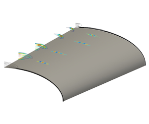
Figure 11(b) presents a three-dimensional reconstruction of the flow in the streamwise direction using the five streamwise locations analysed previously. At each one of these locations, the structures corresponding to the maximum value of  $G(t)$ are interpolated to create the three-dimensional perturbation flow field. Note that the amplitude of the structures decays with increasing distance from the centreline. Further, the time at which the maximum value of
 $G(t)$ is reached at each of these five planes is different. For these reasons, the weakest structures that are encountered far from the centreline appear to vanish further downstream. Nevertheless, all structures in the three-dimensional reconstruction shown in figure 11(b) are aligned along the streamwise direction and, as such, they are analogous qualitatively with the crossflow disturbances documented in the experiment of Borg et al. (Reference Borg, Kimmel and Stanfield2012). This confirms the findings of our earlier work (Quintanilha et al. Reference Quintanilha, Belesiotis, Theofilis and Hanifi2018) based on the local stability theory, in which the existence of algebraically-growing streamwise-aligned structures on the elliptic cone surface was documented. These crossflow-like disturbances are found here as well to be transiently more amplified than the modally unstable centreline structures. Such a conversion of linear optimal perturbations to crossflow modes has been seen in both incompressible and compressible boundary layers (Tempelmann et al. Reference Tempelmann, Hanifi and Henningson2010, Reference Tempelmann, Hanifi and Henningson2012). On the elliptic cone, the streamwise-aligned structures are concentrated in the close proximity of the centreline vortex and quickly decay towards the leading edge. Calculation of steady laminar basic states was reported to be challenging on account of vortices developing as the resolution was increased in the direct numerical simulations of Dinzl & Candler (Reference Dinzl and Candler2017). Other configurations in which strong transient growth affects the convergence of laminar solutions have also been reported in the literature (e.g. Alves et al. Reference Alves, Santos, Cerulus and Theofilis2019; Cerulus et al. Reference Cerulus, Dos Santos, Quintanilha, Alves and Theofilis2020).
During the recent HIFiRE-5b flight test, transition was measured for  $Re_x > 3.5 \times 10^6$ for free stream Mach number 7.8 (Kimmel et al. Reference Kimmel, Adamczak, Borg, Jewell, Juliano, Stanfield and Berger2019), and the transition front was found to correlate with stationary crossflow modal amplification (Tufts et al. Reference Tufts, Gosse and Kimmel2018b). Therefore, the boundary layer can be assumed to remain laminar over the vehicle during flight at the present 33 km altitude conditions. This indicates that the transient growth reported here was not the dominant source of transition. However, a different excitation spectrum (larger free stream disturbances or wall roughness) might lead to transient-growth-induced transition. Thus the present analysis may be more relevant to noisy wind tunnel testing where transition has been measured at Mach 6 for
 $Re_x < 1.5 \times 10^6$ (Kimmel et al. Reference Kimmel, Adamczak, Borg, Jewell, Juliano, Stanfield and Berger2019).
4.3.4. Non-modal analysis of streamwise periodic perturbations
Solutions of the IVP (2.2) have also been obtained at non-zero streamwise wavenumber parameters; of these, representative results obtained at  $\alpha =0.2$, corresponding to a non-dimensional wavelength
 $2 {\rm \pi}/ 0.2 = 31.4$ – the dimensional values being
 $6.8$ mm at 21 km altitude and
 $16.1$ mm at 33 km altitude – are discussed in what follows. Results in figure 12 exhibit the same qualitative behaviour seen at
 $\alpha =0$, namely that a non-negligible initial growth of energy is present, followed by exponential growth or decay of the signal according to modal theory. However, the optimal gain obtained at all parameters examined is
 $G_{opt}=O(10^2)$, one order of magnitude smaller than the maximum gain obtained in the case of streamwise-aligned structures,
 $\alpha =0$.
Comparison of energy gain between 21 km and 33 km altitudes with  $\alpha =0.2$ for different streamwise positions: (a)
 $x^* = 0.36$ m, (b)
 $x^* = 0.42$ m, (c)
 $x^* = 0.52$ m, and (d)
 $x^* = 0.62$ m.

Interestingly, while at all  $x^* \ge 0.4$ m the ultimate behaviour of the
 $G(t)$ curve is one of modal growth, at
 $x^* = 0.36$ m it can be seen that the IVP solution at 21 km and 25 km yields qualitatively different results at asymptotically large times compared to the altitudes of 28 km and 33 km: while at the lower two altitudes modal instability governs the large time behaviour of the solution, at the higher two altitudes the flow is modally stable, and only the transient energy growth may account for linear instability and laminar–turbulent transition. In other words, at 21 km altitude the flow is modally unstable featuring the largest amplification rate. As altitude is increased and the density and Reynolds number decrease, the modal amplification rate also decreases, the flow being modally near-neutral at 28 km, while at the highest altitude of 33 km, all modal perturbations with
 $\alpha =0.2$ are damped. This phenomenon is rather short-lived (it occurs only up to
 $x^* = 0.36$ m) and takes place within a small window. Further downstream, the modal growth dominates all the way until the end of the model surface. As mentioned before, this result is representative of others obtained at different wavenumbers, the quantitative difference being the altitude at which the respective wavenumber becomes modally stable. This finding highlights the importance of performing not only a modal analysis but a full non-modal analysis to interrogate the flow over the HIFiRE-5 elliptic cone model.
Figures 13 and 14 show the initial linear optimal conditions for the density and the streamwise velocity  $\hat {u}$, respectively, at non-dimensional wavenumber
 $\alpha =0.2$, corresponding to a streamwise wavelength of
 $L_x = 16.1$ mm. Overall, results analogous to those at
 $\alpha =0$ are obtained: the initial and optimal disturbances at
 $t=0$ and
 $t=t_{opt}$, respectively, are found to peak in the crossflow region of the cone, while at asymptotically large times, the peak of the perturbations has moved to the cone centreline and can be related to the structures recovered from the solution of the EVP. While the
 $\alpha =0$ and
 $\alpha \ne 0$ results are qualitatively identical at all
 $\alpha$ values examined, the major quantitative difference of the present results from those discussed in § 4.3.2 is in the level of maximum transient energy gain attained. The value of
 $G_{max}$ of the streamwise-aligned structures at any streamwise position along the cone is between two and three orders of magnitude larger than that corresponding to any
 $\alpha \ne 0$ structure. Consequently, non-modal transition on the elliptic cone is expected to be associated with streamwise-aligned structures.
Real part of perturbation density  $\hat {\rho }_r$ with
 $\alpha =0.2$ (
 $L_x = 16.1$ mm). The first column (a–d) corresponds to the optimal initial condition
 $t=0$; the middle column (e–h) corresponds to the associated optimal perturbation
 $t=t_{opt}$; and the right column (i–l) corresponds to the long time behaviour
 $t \rightarrow \infty$. Each row corresponds to a different streamwise location along the elliptic cone surface, namely
 $x^* = 0.36$ m (a,e,i),
 $x^* = 0.42$ m (b, f, j),
 $x^* = 0.52$ m (c,g,k) and
 $x^* = 0.62$ m (d,h,l). The black isolines correspond to contours of the steady base flow (
 $\bar {u} = 0$ and 0.95).

Real part of streamwise perturbation  $\hat {u}_r$ with
 $\alpha =0.2$ (
 $L_x=16.1$ mm). The first column (a–d) corresponds to the optimal initial condition
 $t=0$; the middle column (e–h) corresponds to the associated optimal perturbation
 $t=t_{opt}$; and the right column (i–l) corresponds to the long time behaviour
 $t \rightarrow \infty$. Each row corresponds to a different streamwise location along the elliptic cone surface, namely
 $x^* = 0.36$ m (a,e,i),
 $x^* = 0.42$ m (b,f,j),
 $x^* = 0.52$ m (c,g,k) and
 $x^* = 0.62$ m (d,h,l). The black isolines correspond to contours of the steady base flow (
 $\bar {u} = 0$ and 0.95).

4.4. Non-modal stability analysis of the attachment line
Results shown in the previous subsections have been obtained on the domain shown on the left of figure 1; in this subsection, non-modal instability analysis is performed on the rightmost of the domains shown in the same figure, which includes the attachment line and an appreciable part of the surface of the elliptic cone.
Figure 15(a) presents energy gain curves at 33 km altitude and at a single location  $x^*=0.52$ m. The streamwise wavenumber
 $\alpha$ is investigated in the range 0–2, corresponding to streamwise periodicity lengths of 16.1 mm to 1.6 mm, respectively. At this altitude, it can be seen that transient energy growth is present over a wide range of wavenumbers, either side of
 $\alpha =1.1$. The level of
 $G_{opt}$ attained is comparable to that seen for streamwise periodic disturbances in the crossflow region of the cone, and typically one to two orders of magnitude lower than that corresponding to the spanwise-periodic streamwise-aligned structures discussed in § 4.3.2; ultimately, as time increases past the respective linear optimal value, the asymptotic dependence of the curves is governed by the respective damped or near-neutral eigenvalues. On the other hand, the gain curve at
 $\alpha =1.1$, as well as at nearby values of this wavenumber parameter not shown here for brevity, is seen to lock on modal dependence early on, the slope of the
 $G(t)$ curve being identical with that predicted by modal analysis.
(a) Gain  $G(t)$ calculated via SVD (solid lines) compared with the slope of the most unstable eigenvalue calculated via the EVP analysis (dashed lines) at
 $x^* = 0.52$ m and 33 km altitude. (b) The associated
 $\omega _i$ vs
 $\alpha$ curve showing the modally unstable region.

The maximum transient energy gain found along the attachment line in the present hypersonic flow is substantially smaller than that reported by Obrist & Schmid (Reference Obrist and Schmid2003) on the swept Hiemenz model of the attachment line in the incompressible limit. It may be conjectured that this is due to either or both of flow compressibility and surface curvature in the vicinity of the cone major axis, curvature having been found to have a stabilizing effect on this class of flows by Lin & Malik (Reference Lin and Malik1997) also in the incompressible regime. However, verification of this conjecture is beyond the scope of the present analysis and will be undertaken in a separate study.
5. Summary and conclusions
Linear transient growth analysis is presented on the aspect ratio 2 elliptic cone modelling the HIFiRE-5 geometry in hypersonic flow at Mach numbers between 7.45 and 8.05 (unit Reynolds number between  $1.07\times 10^7$ and
 $1.89\times 10^6$) corresponding to flight altitudes 21 km and 33 km, respectively. Solutions to the IVP are obtained by solving the SVD of the matrices discretizing the EVP. Convergence of the IVP results was found to require eigenspectra comprising an orders of magnitude larger number of modes than the corresponding modal analysis. A novel massively parallel solver for complex non-symmetric generalized EVPs in generalized coordinates was developed for the numerical work. Validation was performed by recovering, as leading members of the eigenspectra used in the reconstruction of the solution to the IVP, modal stability analysis results known from the earlier analysis of Paredes et al. (Reference Paredes, Gosse, Theofilis and Kimmel2016). For reasons of numerical feasibility, the vicinity of the centreline and the crossflow region have been analysed separately from the attachment line region, so that numerical convergence could be ensured and the underlying physical phenomena could be adequately captured in both of these domains.
Guided by solutions to the local transient growth problem, which indicated that streamwise-aligned linear perturbations exhibit the highest energy gain, the two-dimensional IVP has been solved at streamwise stations  $0.36\ {\rm m} \le x^* \le 0.62\ {\rm m}$ along the cone, for a priori unknown time horizons, until the slope of the energy gain curve locked onto the corresponding modal analysis result. In the centreline and crossflow region, substantially larger,
 $G_{opt}=O(10^4)$, transient energy growth is obtained for streamwise-aligned,
 $\alpha =0$, perturbations at both extreme altitudes at the two flight altitudes, compared to
 $G_{opt}=O(10^2)$ obtained for wave-like,
 $\alpha \ne 0$, perturbations. The linear optimal disturbances identified in the present analysis at
 $\alpha =0$ peak in the region of crossflow and vanish towards the attachment line. They take the form of a finite number of isolated elongated structures aligned with the streamwise direction. In the vicinity of the attachment line, the solution to the IVP reveals modal growth around discrete streamwise wavenumber values and feeble algebraic energy growth between these wavenumbers.
A counter-intuitive and relevant result of the present analysis is associated with the variation of the maximum transient energy gain with flight altitude: at any given streamwise location on the cone,  $G_{opt}$ increases monotonically with increasing altitude and decreasing Reynolds number. At the lowest altitude (relatively modest) algebraic/transient energy growth is followed by exponential/modal growth of perturbations at all parameters examined; in other words, the linear instability of the flow is governed by the analysis of the modal scenario discussed by Paredes et al. (Reference Paredes, Gosse, Theofilis and Kimmel2016). By contrast, at 33 km, transient growth is on occasion followed by modal/exponential decay of the perturbations in question, implying that as the flight altitude increases, transient growth becomes the only physical linear instability mechanism leading the hypersonic boundary layer flow to laminar–turbulent transition. By contrast to the quadratic dependence of the maximum energy gain on the local Reynolds number at the lower altitude/higher Reynolds number, a quartic dependence
 $G_{opt}\sim Re_x^4$ was found in the highest altitude case, indicating that laminar–turbulent transition of hypersonic boundary layer flow may arise from non-modal mechanisms, which presently remain unexplored for the majority of flows of interest.
Acknowledgements
The US Government is authorized to reproduce and distribute reprints for Governmental purpose notwithstanding any copyright notation thereon. Discussions with Dr R. Kimmel and Dr R. Gosse, who also made available the base flow analysed herein, are gratefully acknowledged. Access to Copper Cray XE6m (https://www.ors.hpc.mil) was made possible by project AFVAW10102F62, with Dr N. Bisek as Principal Investigator, who is gratefully acknowledged.
Funding
Effort sponsored by the Air Force Office of Scientific Research, Air Force Material Command, USAF, under grant no. FA9550-15-1-0387, ‘Global transient growth mechanisms in high-speed flows, with application to the elliptic cone’, monitored by Dr ‘Pon’ R. Ponnappan and Dr I. Leyva.
Declaration of interests
The authors report no conflict of interest.


 Open access

