





1. Introduction
In modern combustion systems, the bidirectional coupling between unsteady heat release and acoustic waves can give rise to self-excited flow oscillations, termed thermoacoustic instabilities (Poinsot Reference Poinsot2017; Polifke Reference Polifke2020; Schuller et al. Reference Schuller, Poinsot and Candel2020). These instabilities can manifest at high amplitudes and across multiple natural frequencies and mode shapes, leading to detrimental consequences (O’Connor et al. Reference O’Connor, Acharya and Lieuwen2015; Juniper & Sujith Reference Juniper and Sujith2018; Sujith & Pawar Reference Sujith and Pawar2021). In gas turbines, they can cause blade fatigue, excessive heat transfer, elevated pollutant emissions and flame blow-off, necessitating costly maintenance and repairs (Lieuwen & Yang Reference Lieuwen and Yang2005). In rocket engines, they pose a critical safety hazard that can result in catastrophic mission failure (Yang & Anderson Reference Yang and Anderson1995). The ongoing transition towards carbon-free fuels, particularly hydrogen and ammonia, in electricity generation and aviation presents additional challenges for existing predictive and control methodologies (Morgans & Yang Reference Morgans and Yang2025).
1.1. Strategies for controlling thermoacoustic instabilities
Methods for mitigating thermoacoustic instabilities fall into two fundamental categories: passive control and active control (Candel Reference Candel2002; Dowling & Morgans Reference Dowling and Morgans2005). Both categories aim to enhance acoustic/viscous dissipation and/or suppress thermoacoustic driving – the latter arising from physical mechanisms such as hydrodynamic instabilities, equivalence-ratio coupling, and entropy waves (Lieuwen & Yang Reference Lieuwen and Yang2005; Huang & Yang Reference Huang and Yang2009; Poinsot Reference Poinsot2017). Passive control is simple in principle, requiring no external energy or actuators, and can be implemented in various ways, such as optimising the convective time scale of the reactants in a fuel injection system (Lieuwen & Zinn Reference Lieuwen and Zinn1998) or incorporating acoustic damping devices, notably perforated liners (Eldredge & Dowling Reference Eldredge and Dowling2003) or Helmholtz resonators (Dupere & Dowling Reference Dupere and Dowling2005; Zhao & Morgans Reference Zhao and Morgans2009). However, effective implementation of passive control demands a thorough understanding of the diverse flow phenomena and their coupled interactions within combustors, including vortex dynamics, turbulent combustion, heat transfer, and acoustic wave generation, propagation and reflection (Poinsot Reference Poinsot2017; Morgans & Yang Reference Morgans and Yang2025). This understanding remains incomplete due to the inherent sensitivity and nonlinearity of the multiscale flow–acoustic–combustion interactions in the thermoacoustic feedback loop (Ducruix et al. Reference Ducruix, Schuller, Durox and Candel2003; Juniper & Sujith Reference Juniper and Sujith2018; Schuller et al. Reference Schuller, Poinsot and Candel2020).
Active control exploits external energy inputs to disrupt the thermoacoustic feedback loop (McManus et al. Reference McManus, Poinsot and Candel1993), and can be implemented in either open-loop or closed-loop configurations (Zhao et al. Reference Zhao, Lu, Zhao, Li, Wang and Liu2018). Open-loop control (OLC) – which involves predetermined actuation without real-time sensing – has been demonstrated in various combustion systems through modulation of the fuel or air flow rate (Richards et al. Reference Richards, Thornton, Robey and Arellano2007; Ćosić et al. Reference Ćosić, Bobusch, Moeck and Paschereit2012) and direct acoustic forcing of the reaction zones (Bellows et al. Reference Bellows, Hreiz and Lieuwen2008). Recent studies have focused on characterising the nonlinear dynamics and forced synchronisation of self-excited thermoacoustic oscillations under external time-periodic actuation (Balusamy et al. Reference Balusamy, Li, Han, Juniper and Hochgreb2015; Guan et al. Reference Guan, Gupta, Kashinath and Li2019a
). Studies have also established the efficacy of two-frequency forcing (Ćosić et al. Reference Ćosić, Bobusch, Moeck and Paschereit2012) and transient forcing (Guan et al. Reference Guan, He, Murugesan, Li, Liu and Li2019c
) in attenuating thermoacoustic instabilities. Crucially, OLC has been shown to operate through the universal mechanism of asynchronous quenching (AQ) (Guan et al. Reference Guan, Gupta, Kashinath and Li2019a
; Roy et al. Reference Roy, Mondal, Pawar and Sujith2020). In this nonlinear process, time-periodic forcing applied at a frequency far from the natural mode of a self-excited oscillator (i.e. at large detuning) induces phase trajectory collapse from a limit cycle to a stable fixed point (Minorsky Reference Minorsky1967). This results in a substantial amplitude reduction of the forced self-excited system without resonant amplification of the forcing signal itself (Balanov et al. Reference Balanov, Janson, Postnov and Sosnovtseva2009; Kushwaha et al. Reference Kushwaha, Worth, Dawson, Gupta and Li2022). In combustion systems, external forcing applied near the preferred mode of the flame, but far from the natural thermoacoustic mode, can suppress the latter by disrupting the phase synchronisation between pressure and heat-release-rate (HRR) fluctuations (Roy et al. Reference Roy, Mondal, Pawar and Sujith2020). Such synchronisation and quenching phenomena, including AQ and phase/frequency locking, have been successfully reproduced using low-order oscillator models perturbed by a harmonic forcing term (Dewan Reference Dewan1972; Mondal et al. Reference Mondal, Pawar and Sujith2019; Guan et al. Reference Guan, Gupta, Kashinath and Li2019a
). However, although OLC can be effective without detailed system knowledge, it requires lengthy trial-and-error mapping to determine the optimal actuation policy, which can often prove highly sensitive to variations in the operating and boundary conditions. To enhance adaptability, researchers have applied closed-loop control, which incorporates feedback via sensors, actuators and a controller (Candel Reference Candel1992; McManus et al. Reference McManus, Poinsot and Candel1993; Jones et al. Reference Jones, Lee and Santavicca1999; Candel Reference Candel2002; Docquier & Candel Reference Docquier and Candel2002; Dowling & Morgans Reference Dowling and Morgans2005). Conventional closed-loop controllers rely on several distinct approaches. These include phase-shift and time-delay techniques (Seume et al. Reference Seume, Vortmeyer, Krause, Hermann, Hantschk, Zangl, Gleis, Vortmeyer and Orthmann1998; Zhang et al. Reference Zhang, Li, Cheng and Li2020), adaptive model-based controllers (Evesque et al. Reference Evesque, Dowling and Annaswamy2003; Riley et al. Reference Riley, Park, Dowling, Evesque and Annaswamy2004) and frequency-domain loop-shaping controllers based on Nyquist or
 $\mathcal{H}_{\infty }$
principles (Morgans & Stow Reference Morgans and Stow2007; Morgans & Dowling Reference Morgans and Dowling2007). Robustness to modelling uncertainty and changes in operating condition can be pursued via suitably designed Nyquist and
 $\mathcal{H}_{\infty }$
approaches (Hong et al. Reference Hong, Yang and Ray2000; Campos-Delgado et al. Reference Campos-Delgado, Zhou, Allgood and Acharya2003; Morgans & Stow Reference Morgans and Stow2007). By contrast,
 $\mathcal{H}_2$
formulations are primarily associated with optimal control rather than robustness. Such approaches nevertheless require a sufficiently representative model of the system (plant). Although suitable models can be developed for simple combustors undergoing a periodic limit cycle (Dowling & Morgans Reference Dowling and Morgans2005), it is challenging to do so for combustors undergoing quasiperiodic or chaotic thermoacoustic oscillations, because these suffer from more degrees of freedom, greater sensitivity to noise and frequency crosstalk, and the possibility of multiple unstable modes – all coupled through a range of time delays (Duriez et al. Reference Duriez, Brunton and Noack2017). Even if a representative system model can be identified, one still needs to design a controller for it. Conventional feedback controllers are designed to operate in the linear limit near a fixed point or a limit-cycle attractor, not for complex nonlinear dynamics such as quasiperiodicity and chaos (Duriez et al. Reference Duriez, Brunton and Noack2017). For these reasons, we take an alternative approach to designing a closed-loop controller for aperiodic thermoacoustic oscillations, one that leverages data-driven machine learning to avoid the need for a system model.
1.2. Aperiodic thermoacoustic oscillations and their control
Thermoacoustic oscillations can take on many different forms, such as limit-cycle orbits (Kashinath et al. Reference Kashinath, Li and Juniper2018; Guan et al. Reference Guan, Gupta, Kashinath and Li2019a ; Yin et al. Reference Yin, Yang, Guan, Redonnet, Gupta and Li2024), quasiperiodic motion on a torus attractor (Kashinath et al. Reference Kashinath, Li and Juniper2018; Guan et al. Reference Guan, Gupta, Wan and Li2019b ; Sato et al. Reference Sato, Hyodo, Biwa and Delage2020) or chaotic dynamics on a strange attractor (Delage et al. Reference Delage, Takayama and Biwa2017; Guan et al. Reference Guan, Murugesan and Li2018b ; Kashinath et al. Reference Kashinath, Li and Juniper2018; Guan et al. Reference Guan, Yin, Yang and Li2024). Although much research has been conducted on controlling thermoacoustic oscillations, most of it has targeted fixed-point or periodic limit-cycle oscillations. However, it is important to recognise that aperiodic oscillations can also occur (Guan et al. Reference Guan, Liu, Jin, Gupta and Li2018a , Reference Guan, Li, Ahn and Kim2019d , Reference Guan, Gupta and Li2020; Sujith & Pawar Reference Sujith and Pawar2021). Indeed, aperiodic regimes can occupy substantial regions of parameter space in thermoacoustic systems owing to nonlinear mode interactions and hydrodynamic–acoustic–flame coupling (Sujith & Pawar Reference Sujith and Pawar2021). They can be especially challenging to diagnose and suppress because their spectra combine broadband and discrete components, with dynamics that are exceptionally sensitive to initial conditions. The present study focuses on the control of aperiodic thermoacoustic oscillations, encompassing both quasiperiodic (with two incommensurate modes on a two-torus) and chaotic dynamics.
In nonlinear dynamical systems, quasiperiodicity can arise from the coexistence of two or more incommensurate periodic modes, leading to an oscillation period of infinity (Li & Juniper Reference Li and Juniper2013a ). In phase space, a quasiperiodic system evolves along a non-repeating trajectory on a two-dimensional (2-D) torus attractor formed by the two periodic modes (Thompson & Stewart Reference Thompson and Stewart2002). In the field of thermoacoustics, Kashinath et al. (Reference Kashinath, Li and Juniper2018) numerically investigated the forced synchronisation of a 2-D slot-stabilised laminar premixed flame exhibiting quasiperiodic and chaotic dynamics. On the experimental front, Guan et al. (Reference Guan, Gupta, Wan and Li2019b ) and Sato et al. (Reference Sato, Hyodo, Biwa and Delage2020) examined the effects of periodic acoustic forcing on quasiperiodic thermoacoustic oscillations within a synchronisation framework. Quasiperiodicity has been observed not only in thermoacoustic systems but also in various other flow systems, including the wake of bluff bodies (Baek & Sung Reference Baek and Sung2000), wavy-channel convection (Doranehgard et al. Reference Doranehgard, Borazjani, Karimi and Li2024a , Reference Doranehgard, Karimi, Borazjani and Lib ), jet diffusion flames (Li & Juniper Reference Li and Juniper2013b ) and globally unstable jets (Li & Juniper Reference Li and Juniper2013a ; Shoji et al. Reference Shoji, Harris, Besnard, Schein and Karagozian2020; Kushwaha et al. Reference Kushwaha, Worth, Dawson, Gupta and Li2026).
Chaotic oscillations are far more complex than periodic and quasiperiodic oscillations. Their dynamics may encompass various incommensurate frequencies, broadband spectral features, time-dependent amplitudes and low-dimensional strange attractors (Balanov et al. Reference Balanov, Janson, Postnov and Sosnovtseva2009; Sujith & Unni Reference Sujith and Unni2021). Kabiraj et al. (Reference Kabiraj, Saurabh, Wahi and Sujith2012) demonstrated that a chaotic state can emerge through quasiperiodic tori breakdown – known as the Ruelle–Takens–Newhouse (RTN) route – in a ducted laminar premixed flame. Kashinath et al. (Reference Kashinath, Waugh and Juniper2014) explored the bifurcations of a
 $G$
-equation flame under different operating conditions and found two classic routes to chaos: the period-doubling route and the RTN route. Delage et al. (Reference Delage, Takayama and Biwa2018) examined the dynamics of two coupled chaotic thermoacoustic oscillators that are dissipatively coupled and observed a similar RTN route to chaos. Guan et al. (Reference Guan, Murugesan and Li2018b
, Reference Guan, Li, Ahn and Kim2019d
, Reference Guan, Yin, Yang and Li2024) investigated the chaotic dynamics of a forced self-excited laminar combustor and an aeroengine system, which included identifying the type-II intermittency route to chaos in the former (Guan et al. Reference Guan, Gupta and Li2020). Chaotic signatures have been observed in combustion noise, and the departure from chaos has been proposed as an early warning signal of impending thermoacoustic instabilities (Nair et al. Reference Nair, Thampi, Karuppusamy, Gopalan and Sujith2013). Complex networks have been used to analyse the transition from combustion noise (chaos) to thermoacoustic instability (limit cycle) through intermittency (Tandon & Sujith Reference Tandon and Sujith2021). Passive control techniques have been used to optimise the design of heat-source parameters for suppressing chaotic thermoacoustic oscillations (Huhn & Magri Reference Huhn and Magri2020). In addition to analysing individual oscillators, researchers have also examined coupled oscillator systems, revealing the influence of quasiperiodic modulations on coupled chaotic dynamics (Agrawal et al. Reference Agrawal, Prasad and Ramaswamy2010) and identifying on–off intermittency in coupled chaotic oscillators (Delage et al. Reference Delage, Takayama and Biwa2017). However, the active control of aperiodic thermoacoustic oscillations remains largely unexplored due to their highly nonlinear, multimode nature.
1.3. Genetic programming for flow control
Machine learning has gained broad traction in the field of flow control, complementing traditional optimisation strategies (Duriez et al. Reference Duriez, Brunton and Noack2017; Brunton et al. Reference Brunton, Noack and Koumoutsakos2020; Kimishima et al. Reference Kimishima, Yin, Doranehgard, Gupta and Li2025). Specifically, evolutionary algorithms, such as genetic algorithms and genetic programming (GP), have shown particular promise as data-driven control frameworks (Koza Reference Koza1992; Koza et al. Reference Koza, Bennett and Stiffelman1999; Duriez et al. Reference Duriez, Brunton and Noack2017). Such evolutionary tools have found success in various flow-control applications, including suppressing recirculation zones behind backward-facing steps (Gautier et al. Reference Gautier, Aider, Duriez, Noack, Segond and Abel2015; Benard et al. Reference Benard, Pons-Prats, Periaux, Bugeda, Braud, Bonnet and Moreau2016; Chovet et al. Reference Chovet, Keirsbulck, Noack, Lippert and Foucaut2017), manipulating mixing layers (Parezanović et al. Reference Parezanović2015, Reference Parezanović, Cordier, Spohn, Duriez, Noack, Bonnet, Segond, Abel and Brunton2016; Li et al. Reference Li, Tan, Gao and Noack2020), shrinking separated-flow zones (Debien et al. Reference Debien, Von Krbek, Mazellier, Duriez, Cordier, Noack, Abel and Kourta2016; Passaggia et al. Reference Passaggia, Quansah, Mazellier, Maceda and Kourta2022), reducing drag (Li et al. Reference Li, Noack, Cordier, Borée and Harambat2017; Minelli et al. Reference Minelli, Dong, Noack and Krajnović2020; Qiao et al. Reference Qiao, Minelli, Noack, Krajnović and Chernoray2021; Zigunov et al. Reference Zigunov, Sellappan and Alvi2021; Castellanos et al. Reference Castellanos, Cornejo Maceda, de la Fuente, Noack, Ianiro and Discetti2022; Qiao et al. Reference Qiao, Minelli, Noack, Krajnović and Chernoray2023; Chen et al. Reference Chen, Zong, Song, Wu, Liang and Su2024), stabilising wakes downstream of rotating cylinders (Raibaudo et al. 2017, 2020; Raibaudo & Martinuzzi Reference Raibaudo and Martinuzzi2021), enhancing turbulent jet mixing (Wu et al. Reference Wu, Fan, Zhou, Li and Noack2018; Zhou et al. Reference Zhou, Fan, Zhang, Li and Noack2020; Perumal et al. Reference Perumal, Wu, Fan and Zhou2022; Zigunov et al. Reference Zigunov, Sellappan and Alvi2022), mitigating vortex-induced vibrations (Ren et al. Reference Ren, Wang and Tang2019) and suppressing combustion instabilities (Liu et al. Reference Liu, Tan, Li, Hou, Zhang and Noack2023; Yin et al. Reference Yin, Yang, Guan, Redonnet, Gupta and Li2024; Yin & Li Reference Yin and Li2025). Given that GP can explore a larger search space than genetic algorithms owing to its ability to optimise both the control-law structure and its parameters (Koza Reference Koza1992; Koza et al. Reference Koza, Bennett and Stiffelman1999), we apply GP in the present study – in both open-loop and closed-loop forms – to suppress aperiodic thermoacoustic oscillations.
Previous experiments have demonstrated the superiority of evolutionary algorithms, particularly GP, over conventional active control strategies. For instance, by applying GP actuation to the recirculation zone of a backward-facing-step flow, Chovet et al. (Reference Chovet, Keirsbulck, Noack, Lippert and Foucaut2017) were able to reduce the external separation length by up to 8.6 % (compared with 5.3 % with conventional periodic actuation) and to extend the corresponding internal value by 70.6 % (compared with 37.9 %). Using GP, Ren et al. (Reference Ren, Wang and Tang2019) achieved a 94.2 % reduction in the vortex-induced-vibration amplitude of a round rod, surpassing the performance of the best open-loop actuation policy by 21.4 %. Besides its superior metrics, GP has the potential to learn novel actuation mechanisms. For example, for flow separation control, Gautier et al. (Reference Gautier, Aider, Duriez, Noack, Segond and Abel2015) used GP to discover an actuation mechanism unlike typical open-loop strategies: instead of exciting the typical Kelvin–Helmholtz instability, GP showed better performance by exciting the low frequencies of the recirculation region. In the context of maximising the mixing rate of turbulent jets, GP can self-learn promising spatiotemporal actuation policies (e.g. axisymmetric, helical and flapping perturbations), uncovering previously unreported actuation patterns such as the so-called combined mode (Zhou et al. Reference Zhou, Fan, Zhang, Li and Noack2020). To date, most GP studies have focused on closed-loop (feedback) control, but more recent studies have looked at OLC as well. For instance, Li et al. (Reference Li, Tan, Gao and Noack2020) numerically destabilised and stabilised a mixing layer using GP in an open-loop set-up, and Perumal et al. (Reference Perumal, Wu, Fan and Zhou2022) introduced a modified GP algorithm with time-independent open-loop functions to form a hybrid artificial intelligence strategy to enhance jet mixing.
In the field of thermoacoustics, Liu et al. (Reference Liu, Tan, Li, Hou, Zhang and Noack2023) demonstrated a 67.1 % suppression of periodic thermoacoustic oscillations in a premixed combustor controlled by GP. Building on that work, we recently implemented a GP framework for thermoacoustic suppression in two complementary periodic systems. In a laminar flame-driven Rijke tube (Yin et al. Reference Yin, Yang, Guan, Redonnet, Gupta and Li2024), we applied GP in both closed-loop and open-loop forms. By benchmarking GP closed-loop control (GCC) against GP open-loop control (GOC) and conventional OLC with time-periodic actuation, we found that all three strategies can effectively suppress periodic limit-cycle oscillations, but that GCC achieves the highest efficiency by learning an actuation mechanism that exploits the preferred mode of the flame, identified via the peak gain of the open-flame describing function (FDF). In a turbulent hydrogen–methane combustor (Yin et al. Reference Yin, Ånestad, Æsøy, Worth and Li2026), we applied the same GP methodology to periodic thermoacoustic oscillations in a fundamentally different, high-Reynolds-number system with more degrees of freedom, and found that GCC remains superior in effectiveness and efficiency. In that study (Yin et al. Reference Yin, Ånestad, Æsøy, Worth and Li2026), suppression occurs via synchronous quenching of the natural thermoacoustic mode, accompanied by a disruption of the flame–acoustic coupling (e.g. phase drifting), reduced Rayleigh driving and inhibited large-scale coherent vortex formation.
1.4. Contributions of the present study
The present study extends our recent periodic-regime demonstrations (Yin et al. Reference Young and Householder2024, Reference Yin, Yang, Guan, Redonnet, Gupta and Li2026). We now apply GP to control aperiodic thermoacoustic oscillations (quasiperiodic and chaotic) in a laminar combustor. This extension is non-trivial because aperiodic regimes often feature multimode interactions, broadband spectra with distinct peaks, and extreme sensitivity to initial conditions (Thompson & Stewart Reference Thompson and Stewart2002), so control performance cannot be validated or interpreted using diagnostics designed for periodic limit cycles. We therefore combine GP control with regime-appropriate analyses, including synchronisation metrics, chaos diagnostics based on the 0–1 test and complexity–entropy measures, and modal decomposition techniques to identify individual HRR modes that are otherwise obscured by multimode flame dynamics.
Although our previous study (Yin et al. Reference Yin, Yang, Guan, Redonnet, Gupta and Li2024) established the importance of preferred-mode flame receptivity, the present study shows how preferred-mode actuation, multimode interactions and synchronisation jointly govern thermoacoustic suppression in the quasiperiodic and chaotic regimes, including cases in which the dominant mode in the controlled state exists far from the natural mode and, for quasiperiodicity, can yield a GP-suppressed state that persists even after control deactivation.
Our objective is threefold. First, we test whether GCC can effectively suppress self-excited quasiperiodic and chaotic thermoacoustic oscillations. Second, we seek to identify and validate the physical mechanisms underpinning suppression in these aperiodic regimes by analysing the GP-discovered actuation signals together with the resulting multimode flame and acoustic dynamics, using diagnostics tailored to quasiperiodicity and chaos. Third, we benchmark GCC against GOC and conventional OLC in terms of both thermoacoustic attenuation and actuation effort, thereby quantifying the efficiency gains (if any) afforded by closed-loop, model-free GP control in aperiodic thermoacoustics.
Our focus is on generalisation across dynamical regimes rather than across system-specific parameter changes. While geometry or operating-point modifications (e.g. combustor dimensions and/or reactant flow rates) are certainly possible in laboratory settings, they typically produce system-specific changes and do not directly address the broader question of whether a control framework remains effective across nonlinear states commonly encountered in thermoacoustics. Quasiperiodic and chaotic attractors are universal across a wide range of thermoacoustic configurations. Moreover, quasiperiodicity and its breakdown constitute a generic route to chaos, i.e. the RTN scenario (Thompson & Stewart Reference Thompson and Stewart2002). Therefore, demonstrating thermoacoustic suppression in both quasiperiodic and chaotic regimes provides a form of dynamical generalisation that is expected to be transferable across systems exhibiting similar nonlinear behaviour, even when the detailed plant parameters differ.
The rest of this paper is organised as follows. The experimental set-up, operating conditions and GP algorithm are presented in § 2. The application of GP to suppress quasiperiodic and chaotic oscillations is discussed in §§ 3 and 4, respectively, along with the corresponding actuation mechanisms. Finally, the conclusions of this study are summarised in § 5.
2. Experimental set-up and GP control algorithm
We apply GP in both closed-loop and open-loop configurations to suppress aperiodic thermoacoustic oscillations in a flame-driven Rijke tube. The following subsections provide an overview of the experimental set-up, operating conditions and GP control algorithm used in our research.
2.1. Experimental set-up
The experimental set-up, shown in figure 1, is consistent with the configuration used in our prior investigations (Guan et al. Reference Guan, Gupta, Kashinath and Li2019a , Reference Guan, Gupta, Wan and Lib , Reference Guan, He, Murugesan, Li, Liu and Lic , Reference Guan, Yin, Yang and Li2024; Yin et al. Reference Yin, Yang, Guan, Redonnet, Gupta and Li2024). Its design centres around a flame-driven Rijke tube, comprising a central burner tube with an inner diameter of 16.8 mm and a length of 800 mm. Constructed from stainless steel, the burner tube is capped by a copper extension tip with an outlet inner diameter of 12 mm and a length of 30 mm. The extension tip serves to stabilise a laminar premixed flame (liquid petroleum gas (LPG)–air mixture) inside an open–open quartz tube combustor with an inner diameter of 44 mm and a length of 860 mm. For open-loop and closed-loop control, acoustic perturbations are applied to the flame using a loudspeaker (FaitalPRO 6FE100) driven by a power amplifier. The maximum perturbation amplitude is held to approximately 3 % of the actuator limit to avoid flame blow-off. An Arduino board is used for GCC, a LabVIEW module is used for GOC and a function generator is used to generate open-loop harmonic forcing for OLC.
Experimental set-up of a flame-driven Rijke tube subjected to three control strategies: GCC, GOC and OLC. The measurement diagnostics consist of a probe microphone (PM), a photomultiplier tube (PMT), a high-speed camera (HSC) and a data acquisition device (DAQ). The acoustic pressure (
 $p'$
) captured by the PM serves as the primary sensor signal.

The thermoacoustic amplitude, quantified by the instantaneous pressure fluctuations (
 $p'$
) within the combustor, is measured with a PM (GRAS 40SA; sensitivity of 3 mV Pa
 $^{-1} \pm 3$
dB). The instantaneous HRR fluctuations of the flame (
 $q'$
) are measured by monitoring the chemiluminescence emission of CH* using a PMT (Thorlabs PMM01) equipped with a bandpass optical filter (430 nm). Simultaneous recording of the microphone, photomultiplier and loudspeaker input signals is achieved at a sampling rate of 10 kHz using a DAQ (NI USB-6356) for postprocessing. Depending on the equivalence ratio and the flame position within the combustor, this thermoacoustic system can exhibit various types of nonlinear self-excited oscillations. These include period-one limit cycles (Guan et al. Reference Guan, Gupta, Kashinath and Li2019a
,
Reference Guan, He, Murugesan, Li, Liu and Lic
), quasiperiodicity (Guan et al. Reference Guan, Gupta, Wan and Li2019b
), chaos (Guan et al. Reference Guan, Yin, Yang and Li2024) and strange non-chaos (Guan et al. Reference Guan, Murugesan and Li2018b
).
For quasiperiodic oscillations, the flame is located at
 $z/L=0.45$
, where
 $z$
is measured from the bottom of the combustor to the top of the burner extension tip, and
 $L$
is the total combustor length. The volumetric flow rates of air and LPG are
 $10.5$
and
 $0.20$
standard litres per minute, respectively. This yields a bulk reactant velocity of
 $1.6$
m s
 $^{-1}$
(
 $\pm 0.6 \,\%$
), an equivalence ratio of
 $0.57$
(
 $\pm 3.2 \,\%$
), a thermal flame power of
 $390$
W (
 $\pm 4.6 \,\%$
) and a Reynolds number of
 $1300$
(
 $\pm 1.2 \,\%$
). The natural (uncontrolled) quasiperiodic oscillations exhibit dominant modes at two incommensurate frequencies:
 $f_1=251$
and
 $f_2=174 \pm 1.5$
Hz.
For chaotic oscillations, the flame is located at
 $z/L=0.12$
, and the volumetric flow rates of air and LPG are
 $9.5$
and
 $0.14$
standard litres per minute, respectively. This yields a bulk reactant velocity of
 $1.4$
m s
 $^{-1}$
(
 $\pm 0.6 \,\%$
), an equivalence ratio of
 $0.44$
(
 $\pm 3.2 \,\%$
), a thermal flame power of
 $270$
W (
 $\pm 4.6 \,\%$
) and a Reynolds number of
 $1200$
(
 $\pm 1.2 \,\%$
). The natural (uncontrolled) chaotic oscillations exhibit dominant modes at
 $f_1=224 \pm 8$
Hz and
 $f_2=168 \pm 10$
Hz. These operating conditions for quasiperiodicity and chaos are identical to those from our previous studies (Guan et al. Reference Guan, Gupta, Wan and Li2019b
, Reference Guan, Yin, Yang and Li2024).
2.2. The GP control algorithm
The GP control algorithm is partitioned into a fast loop and a slow loop (Duriez et al. Reference Duriez, Brunton and Noack2017). The fast loop is a conventional real-time feedback control loop. The slow loop is for evolutionary discovery of control laws, termed individuals, and consists of three main steps, as illustrated in figure 2: (i) initialising a generation; (ii) evaluating the generation; (iii) breeding further generations. Here, we express the control laws as syntax trees (see bottom left-hand side of figure 2), following the methodology of Koza (Reference Koza1994). The leaves (squares) of the syntax tree correspond to constants or inputs, while the nodes (circles) correspond to basic functions and operators, as summarised in table 1. The complexity of a candidate individual is governed by the depth of its syntax tree, defined as the length of the longest path from the root node to any leaf. To balance model expressiveness with computational efficiency (and to mitigate GP bloat), we constrain the tree depth to between 5 and 12. In line with common GP practice, each candidate individual is screened before experimental evaluation to ensure that it yields real-valued outputs and that the resulting actuation command remains within the safe operating limits of the actuator (Duriez et al. Reference Duriez, Brunton and Noack2017). Individuals that output non-real values (e.g. due to invalid operations) or commands that violate actuator safety limits are discarded and assigned a poor fitness without being tested in the experiments.
Parameters and probabilities of the GP algorithm. Here QP, quasiperiodic; CH, chaotic.

Table 1. Long description
A table with two columns and twelve rows. The first column lists parameters or probabilities, and the second column lists their corresponding values. The parameters and probabilities include the number of generations, size of a generation, number of elite individuals, replication probability, mutation probability, crossover probability, evaluation time, penalisation coefficient, and constant range. The node functions listed are plus, minus, times, divide, sine, cosine, exponential, and logarithm.
The GP control architecture comprising two main loops (Duriez et al. Reference Duriez, Brunton and Noack2017). The slow loop is for evolutionary discovery of individuals, while the fast loop is for real-time feedback control. Here,
 $K^j_i$
is the
 $i$
th individual of the
 $j$
th generation, and
 $J_i^j$
denotes its corresponding cost function.

The output from an individual is an actuation signal that is then fed into the power amplifier (figure 1). The actuation signal is expressed as
 $b^j_{i}=K^j_i(x)$
, where
 $K^j_i$
denotes the
 $i$
th individual of the
 $j$
th generation. For GCC,
 $K^j_i$
is a static nonlinear feedback control law (memoryless input–output map) synthesised by GP and evaluated in real time on the Arduino board. This distinguishes GCC from GOC and OLC, in which
 $b$
is prescribed a priori and does not adapt to the evolving thermoacoustic state. Although
 $K^j_i$
is static, the resulting GCC actuation signal
 $b$
is generally non-trivial because it is continuously modulated by the time-varying measured state:
 $x \equiv p'/ \langle |p_*'|\rangle _T$
. This is defined as the instantaneous pressure fluctuation with control (
 $p'$
) normalised by the average pressure fluctuation amplitude without control (
 $\langle |p_*'|\rangle _T$
). Here,
 $\langle \boldsymbol{\cdot }\rangle _T$
represents time averaging over interval
 $T=2$
s, which was found to be sufficiently long for statistical analysis. Thus, in this study, GCC is implemented as real-time measurement-based feedback control in which the actuation signal is computed online from instantaneous sensor measurements via a state-dependent mapping identified by GP. The signals
 $b$
,
 $x$
and
 $p'$
are time-varying and may be written as
 $b(t)$
,
 $x(t)$
and
 $p'(t)$
, but for brevity, they are denoted simply as
 $b$
,
 $x$
and
 $p'$
hereafter.
To provide a broad initial sampling of the admissible control-law space while keeping the experimental training time practical, we initialise the first generation with
 $N_s=100$
individuals, as per table 1 (Duriez et al. Reference Duriez, Brunton and Noack2017). These first-generation individuals are not manually prescribed; rather, they are generated automatically within the GP search space defined by the allowable node functions, the constant range and the syntax-tree-depth limits in table 1. The node-function set follows prior successful applications of GP to flow control (Gautier et al. Reference Gautier, Aider, Duriez, Noack, Segond and Abel2015; Parezanović et al. Reference Parezanović, Cordier, Spohn, Duriez, Noack, Bonnet, Segond, Abel and Brunton2016; Li et al. Reference Li, Noack, Cordier, Borée and Harambat2017; Wu et al. Reference Wu, Fan, Zhou, Li and Noack2018). Each generated individual is then subject to the physical-admissibility screening described above. In subsequent generations, we reduce the population size to
 $N_s=60$
to reduce the GP training time after this initial broad exploration, while maintaining control performance. Following the initialisation of the first generation of individuals, we evaluate them using the cost function,
 \begin{equation} J \equiv \langle S \rangle _{T_e} + \xi \langle | B' | \rangle _{T_e}, \end{equation}
where
 $T_e = 2$
s is the evaluation time. In this context,
 $S \equiv |x| \equiv |p'|/ \langle |p_*'|\rangle _T$
, and
 $|B'|$
is the voltage fluctuation amplitude into the loudspeaker, after power amplification. The cost function
 $J$
is formulated as the sum of the state cost (i.e. thermoacoustic amplitude,
 $\langle S \rangle _{T_e}$
) and the input cost (i.e. actuator power,
 $\langle | B' | \rangle _{T_e}$
). The balance between performance and economy is determined by the penalisation coefficient
 $\xi$
, where a low (high) value of
 $\xi$
prioritises (sacrifices) performance over economy. Here
 $\xi$
is set as 2 for the quasiperiodic case and 1.5 for the chaotic case. Because
 $J$
explicitly penalises both the residual thermoacoustic amplitude and the actuation effort, differences in the latter are not ancillary but directly affect the controller efficiency. Thus, when two control strategies achieve comparable thermoacoustic attenuation, the strategy with a lower actuation energy requirement can be considered superior under the stated control objective. It is also more attractive for practical deployment where the actuator authority and power budget may be limited.
To evaluate each individual, we use a runtime of 8 s for the quasiperiodic case and 15 s for the chaotic case, with the final
 $T_e = 2$
s used for the calculation of
 $J$
, after which the individual is deactivated. Subsequently, a dwell time of at least 6 s elapses before activating the next individual. These time intervals are chosen to ensure that the controlled system reaches an asymptotic state while allowing the uncontrolled system to return to its natural self-excited state.
The breeding process for the next generation involves ranking all the individuals in the current generation based on their performance measured by
 $J^j_i$
. The new generation consists of three genetic pools: (i) individuals forwarded by elitism, which are top-performing individuals directly carried over without modifications from the current generation; (ii) individuals bred through evolutionary operations such as replication, mutation and crossover; (iii) freshly generated individuals introduced to maintain genetic diversity. Replication entails randomly selecting branches of individuals and forwarding them to the next generation, mutation involves randomly replacing certain branches, and crossover involves randomly selecting two individuals and exchanging some of their branches. The parameters and probabilities used in our GP control implementation can be found in table 1 (Duriez et al. Reference Duriez, Brunton and Noack2017).
3. Results and discussion: GP control of quasiperiodic oscillations
We consider GP control of quasiperiodic thermoacoustic oscillations produced at the same operating conditions as those in our prior work (§ 2.1) (Guan et al. Reference Guan, Gupta, Wan and Li2019b ). We start with GCC and then benchmark the results against GOC and OLC.
3.1. Convergence history of GCC
Figures 3(a) and 3(b) show the GCC convergence history for the quasiperiodic case. As the number of generations progresses from
 $j=1$
to
 $12$
, the number of individuals that achieve low
 $J$
(below
 $0.2$
) increases (figure 3
 $a$
). The
 $J$
values of the top 50 individuals in each generation are displayed, with the final generation (
 $j=12$
) highlighted in red. The rapid convergence of the GP algorithm is further evident in figure 3(
 $b$
), which presents the average
 $J$
of the top 15 individuals in each generation, denoted as
 $\bar {J}^j_{1-15}$
. The value of
 $\bar {J}^j_{1-15}$
quickly settles to a minimum after only the fourth generation. Consequently, for conservativeness, we breed a total of
 $N_g = 12$
generations for the quasiperiodic case, before extracting the optimal GCC individual, defined as the individual with the lowest
 $J$
value.
We note that the distribution of
 $J$
values across the full population need not improve monotonically from one generation to the next. For example, figure 3(
 $a$
) shows that generation
 $7$
contains fewer low-
 $J$
individuals than generation
 $5$
, despite the overall convergence trend. This behaviour is expected because, although elitism retains the best-performing individuals, replication, mutation, crossover and the injection of newly generated individuals continue to explore alternative regions of the control-law search space. In this way, intermediate generations may have a broader or less favourable population-level distribution of
 $J$
, while the best individuals are retained and the evolutionary search continues to converge.
Convergence history for GCC of quasiperiodic oscillations: (
 $a$
) cost function
 $J$
of the individuals in each generation and (
 $b$
) the average
 $J$
of the best 15 individuals in each generation, both shown as the number of generations increases from
 $j=1$
to
 $12$
. In (
 $c$
), the control landscape is presented on a 2-D proximity map containing all the GCC individuals, including the optimal one (magenta square) and the uncontrolled case (black triangle). The input–output actuation curve for the optimal GCC individual is depicted in the inset of (
 $c$
).

Figure 3. Long description
Panel A: A line graph shows the cost function of individuals across different generations, with each generation represented by different symbols and colors. The x-axis is labeled ‘Individual’ and ranges from 1 to 50. The y-axis is labeled ‘J’ and ranges from 0 to 1.5. Panel B: Another line graph displays the average cost function of the best 15 individuals in each generation, with the x-axis labeled ‘Generation’ ranging from 1 to 12 and the y-axis labeled ‘J’ ranging from 0 to 1. Panel C: A scatter plot presents the control landscape on a 2-D proximity map, with the x-axis labeled ‘γa’ and the y-axis labeled ‘γb’. The color gradient represents the cost function ‘J’, ranging from 0.16 to 1.4. The optimal individual is marked with a magenta square, and the uncontrolled case is marked with a black triangle. An inset within Panel C shows the input-output actuation curve for the optimal individual.
To visualise the control landscape, we form a 2-D proximity map (figure 3
 $c$
) using classic multidimensional scaling (Young & Householder Reference Young and Householder1938). This gives a centred representation of points
 $\varGamma =[\gamma _1,\gamma _2,\ldots ,\gamma _{N}]$
with
 $\gamma _1,\gamma _2,\ldots ,\gamma _{N} \in \mathbb{R}^2$
, such that the pairwise distances between individuals approximate their true distances. To quantify the dissimilarity between two individuals,
 $K_m$
and
 $K_n$
(with
 $1 \leqslant m,n \leqslant N$
), we define the matrix
 \begin{equation} D_{m,n}={\big [ \big(B'_{rms,m}-B'_{\textit{rms},n} \big)^2+(\eta _m-\eta _n)^2\big ]}^{1/2}+\alpha |J_m-J_n|, \end{equation}
where
 $\eta \equiv (p'_{\textit{rms}}-p'_{rms,\ast })/p'_{rms,\ast }$
, with
 $p'_{\textit{rms}}$
and
 $p'_{rms,\ast }$
representing the root mean square of the pressure fluctuations with and without control, respectively. The first term in (3.1) captures the difference between two individuals in terms of the actuator power and thermoacoustic amplitude reduction, while the second term penalises disparities in their
 $J$
values. Following Duriez et al. (Reference Duriez, Brunton and Noack2017), we set
 $\alpha =2$
to smooth the control landscape. In figure 3(
 $c$
), each GCC individual is represented by a discrete marker, whose colour indicates its
 $J$
value. The uncontrolled case is represented by a black triangle, serving as the reference baseline. The proximity map unveils a scattered pattern, with the best GCC individuals (i.e. those with low
 $J$
) congregating towards the far right-hand side, while the remaining individuals are distributed on the left-hand side. The optimal GCC individual exhibits a remarkably low value of the cost function (
 $J=0.165$
), and the functional form of its input–output curve is described by the expression
 $b(x) = \exp (\sin (1.7x)+\sin (x)-2x)$
. The functional forms of the top 10 GCC individuals and their input–output curves can be found in Appendix A.
3.2. Actuation mechanisms discovered by GCC
Figure 4 shows the system response to the optimal GCC individual from figure 3. Because self-excited thermoacoustic oscillations arise from the two-way coupling between HRR and pressure fluctuations (Rayleigh Reference Rayleigh1878; Lieuwen & Yang Reference Lieuwen and Yang2005), we examine the evolving phase relationship between
 $q'$
and
 $p'$
in figure 5. Coupled oscillatory signals can exhibit a range of synchronisation dynamics, including phase drifting, slipping, locking and trapping (Pikovsky et al. Reference Pikovsky, Rosenblum and Kurths2003; Thévenin et al. Reference Thévenin, Romanelli, Vallet, Brunel and Erneux2011). In externally forced self-excited systems, phase trapping and slipping have been reported during transitions from phase drifting to locking (Li & Juniper Reference Li and Juniper2013c
; Balusamy et al. Reference Balusamy, Li, Han, Juniper and Hochgreb2015; Kashinath et al. Reference Kashinath, Li and Juniper2018). In an unforced thermoacoustic system undergoing a quasiperiodic route to chaos, Mondal et al. (Reference Mondal, Pawar and Sujith2017) also identified phase locking, intermittent phase locking and phase drifting between the pressure and HRR signals. These prior observations motivate the analysis below, in which the
 $p'$
–
 $q'$
phase relationship is examined in both the uncontrolled state and during the transient and asymptotic stages of GCC. In figures 4 and 5, the evolution of our quasiperiodic system under GCC is presented as five distinct intervals (I–V) according to the stage of control:
Response of the quasiperiodic system to the optimal GCC individual from figure 3: time traces of the (
 $a$
) acoustic pressure fluctuation
 $p'$
, (
 $c$
) normalised HRR fluctuation
 $q'/q'_*$
and (
 $e$
) actuator voltage fluctuation
 $B'$
. The corresponding PSDs are shown in (
 $b$
), (
 $d$
) and (
 $f$
), respectively.

Response of the quasiperiodic system to the optimal GCC individual from figure 3: (
 $a$
) evolution of the phase lag between
 $q'$
and
 $p'$
,
 $\Delta \theta _{qp}=\theta _q-\theta _p$
, and (
 $b$
) evolution of the
 $PLV$
. In interval V,
 $PLV \approx 1$
, indicating persistence of a synchronised state after control deactivation.

-
(i) Interval I. When uncontrolled (i.e. in its natural state,
 $0\lt t\lt 2$
s), the system exhibits
$p'$
and
$q'$
fluctuations at two natural incommensurate frequencies,
$f_1$
and
$f_2$
, as can be seen in their power spectral densities (PSDs, figures 4
b and 4
d). Notably, the
$q'$
mode at the binaural beat frequency (
$f_1-f_2$
) is particularly strong. In figure 5(
$a$
), the inset (
$0.72\leqslant t \leqslant 0.86$
s) reveals that the phase lag between
$q'$
and
$p'$
(
$\Delta \theta _{qp}$
) fluctuates within a bounded range, indicating phase trapping (Aronson et al. Reference Aronson, Ermentrout and Kopell1990). This trapping arises from partial synchronisation between
$q'$
and
$p'$
, where frequency locking occurs without complete phase locking, which is why this state is sometimes referred to as imperfect phase locking (Li & Juniper Reference Li and Juniper2013c
; Penelet & Biwa Reference Penelet and Biwa2013). We also observe
$\Delta \theta _{qp}$
drops in multiples of
$2\pi$
radians, known as intermittent synchronisation or phase slipping (Pikovsky et al. Reference Pikovsky, Rosenblum and Kurths2003). Physically, phase slipping signifies that the frequency locking between
$q'$
and
$p'$
persists for a certain duration until one oscillator momentarily decouples and decelerates, weakening the existing frequency locking (Li & Juniper Reference Li and Juniper2013c
). That oscillator then loses a complete cycle within a short time, manifested as
$2\pi$
drops in
$\Delta \theta _{qp}$
.
-
(ii) Interval II. Upon activating the optimal GCC individual at
$t=2$
s, both
$p'$
and
$q'$
exhibit time-series modulations resembling beating interactions (figures 4
a and 4
c). During this transient stage, the dominant
$p'$
and
$q'$
modes maintain their respective natural frequencies (figures 4
b and 4
d). However, a new mode at
$f_g=(0.79\pm 0.02) f_1$
appears intermittently in both
$p'$
and
$q'$
, particularly in the latter. The PSD of the actuation signal (
$B'$
) is dominated by a strong
$f_1$
mode and a weak
$f_2$
mode, with little sign of the
$f_g$
mode (figure 4
$f$
). In figure 5(
$a$
),
$\Delta \theta _{qp}$
continuously decreases in an unbounded manner. This behaviour, known as phase drifting (Li & Juniper Reference Li and Juniper2013c
), indicates an asynchronous relationship between the two coupled signals. The presence of phase drifting suggests that GCC has disrupted the synchronisation between
$q'$
and
$p'$
(Mondal et al. Reference Mondal, Pawar and Sujith2017). As observed in the inset (figure 5
$a$
:
$3.29\leqslant t \leqslant 3.42$
s), phase drifting in interval II is accompanied by intermittent phase trapping (marked with a dashed square) and occasional phase slipping. The coexistence of phase trapping and drifting signifies that the
$q'$
–
$p'$
relationship switches temporally between weak synchronisation and desynchronisation. -
(iii) Interval III. Following the earlier transient stage of beating-like modulations of
$p'$
and
$q'$
, the amplitude of
$p'$
declines gradually, causing the system to settle into a low-amplitude state. In figures 4(b), 4(d) and 4(f), we observe a change in the dominant frequencies of
$p'$
,
$q'$
and
$B'$
, with their natural modes (
$f_1$
and
$f_2$
) giving way to the new mode at
$f_g$
. Simultaneously, desynchronisation between
$p'$
and
$q'$
occurs, as indicated by the continuation of phase drifting (figure 5
$a$
; inset,
$4.42\leqslant t \leqslant 4.53$
s). -
(iv) Interval IV. The decoupling between
$p'$
and
$q'$
drives the system towards the final low-amplitude state. Eventually, both
$p'$
and
$q'$
, along with
$B'$
, converge on the
$f_g$
mode, although weak signs of the natural modes can still be observed intermittently (figures 4
b, 4
d and 4
f). Notably, the amplitude of
$p'$
becomes appreciably lower than its unforced value (figure 4
$a$
), while the amplitude of
$q'$
decreases only slightly (figure 4
$c$
). In the inset (
$9\leqslant t \leqslant 9.14$
s) of figure 5(
$a$
), we find that
$\Delta \theta _{qp}$
remains nearly constant in time, indicating a state of complete synchronisation known as phase locking (Pikovsky et al. Reference Pikovsky, Rosenblum and Kurths2003; Penelet & Biwa Reference Penelet and Biwa2013). -
(v) Interval V. After GCC is switched off at
$t=10$
s, the system remains in the low-amplitude state reached in interval IV (figures 4
a and 4
c). This suggests that GCC has caused the system to evolve to a different attractor (or a different basin of attraction) characterised by low-amplitude
$p'$
oscillations. In this post-GCC regime, the residual fluctuations in
$p'$
and
$q'$
remain strongly phase synchronised, i.e. their phase difference stays nearly constant in time (figure 5
$a$
). However, this should not be interpreted as the original (natural) thermoacoustic mechanism remaining active. Strong phase synchronisation alone does not imply thermoacoustic growth: self-excited instability requires sufficiently large fluctuation amplitudes and a favourable
$p'$
–
$q'$
coupling such that the cycle-averaged acoustic power input remains positive. In this post-GCC regime (interval V), the system exhibits coherent but weak fluctuations, consistent with a stabilised low-amplitude synchronised state.


To further examine the phase synchronisation between
 $q'$
and
 $p'$
, we compute the phase locking value,
 $PLV \equiv |\sum _{t=1}^N\exp (i\Delta \theta _{qp})|/N$
, where
 $\Delta \theta _{qp}$
is the instantaneous phase lag between
 $q'$
and
 $p'$
, obtained from the corresponding analytic signals (Lachaux et al. Reference Lachaux, Rodriguez, Martinerie and Varela1999; Mondal et al. Reference Mondal, Pawar and Sujith2017; Roy et al. Reference Roy, Mondal, Pawar and Sujith2020). The phase locking value quantifies the magnitude of the mean complex phase difference and spans the range
 $[0,1]$
: values near
 $1$
indicate strong synchronisation with an approximately constant phase difference, whereas values near
 $0$
indicate weak synchronisation with a widely varying phase difference. Figure 5(
 $b$
) shows the phase locking value evolution across intervals I–V. Upon GCC activation at
 $t=2$
s, the phase locking value decreases and varies strongly, in line with a disruption of the intrinsic coupling and the coexistence of phase trapping and drifting during the transient stage. As the system converges to the controlled low-amplitude state (interval IV), the phase locking value rises towards unity, indicating a constant phase lag between
 $p'$
and
 $q'$
. When GCC is deactivated, this phase-locked low-amplitude state persists, with the phase locking value remaining close to unity, consistent with the system remaining on the stabilised attractor reached under GCC.
To understand the origin of the
 $f_g$
mode, we refer to studies by Roy et al. (Reference Roy, Mondal, Pawar and Sujith2020) and Yin et al. (Reference Yin, Yang, Guan, Redonnet, Gupta and Li2024), who demonstrated that the inherent flame dynamics can play a vital role in determining the frequency at which oscillation quenching occurs in forced self-excited thermoacoustic systems. We therefore conduct additional experiments with the combustor removed, enabling the flame to be examined without acoustic feedback. The open flame is subjected to time-periodic acoustic forcing at a range of frequencies (
 $f_f$
) and velocity-perturbation amplitudes (
 $u'/\bar {u}$
). Here,
 $u'$
is the velocity fluctuation amplitude at the burner exit, and
 $\bar {u}$
is the time-averaged bulk velocity. The flame response is characterised by the FDF, which is an amplitude-dependent extension of the flame transfer function (Dowling Reference Dowling1997; Balachandran et al. Reference Balachandran, Ayoola, Kaminski, Dowling and Mastorakos2005; Noiray et al. Reference Noiray, Durox, Schuller and Candel2008). Specifically, the FDF relates the fundamental component of the normalised HRR response at an imposed
 $f_f$
to the normalised velocity perturbation:
 $G \equiv (q'/\bar {q})/(u'/\bar {u})$
. Thus, unlike a linear flame transfer function, the FDF permits the gain and phase of the flame response to vary with the forcing amplitude. The FDF approximation assumes that the response at
 $f_f$
is dominant and that higher harmonics generated by flame nonlinearity have a negligible influence on the overall flame–acoustic dynamics (Dowling Reference Dowling1997; Noiray et al. Reference Noiray, Durox, Schuller and Candel2008).
Figure 6 shows the measured FDF gain. A prominent peak in
 $G$
emerges at
 $f_g$
for low values of
 $u'/\bar {u}$
, indicating that the flame exhibits an exceptionally strong HRR response at this frequency. GCC selects actuation with a spectral component near
 $f_g$
, exploiting this enhanced receptivity: low-power actuation can then yield a substantial reduction in thermoacoustic amplitude, potentially via AQ (Guan et al. Reference Guan, Gupta, Kashinath and Li2019a
; Mondal et al. Reference Mondal, Pawar and Sujith2019; Roy et al. Reference Roy, Mondal, Pawar and Sujith2020). This finding aligns with our previous work on periodic-regime suppression (Yin et al. Reference Yin, Yang, Guan, Redonnet, Gupta and Li2024), where the GP algorithm autonomously discovered an actuation mechanism that exploits the strong HRR amplification of the open flame near its preferred mode.
For a perfectly premixed flame without equivalence-ratio fluctuations, the velocity-to-HRR transfer-function gain is expected to approach unity in the quasisteady limit
 $f_f \rightarrow 0$
(Polifke & Lawn Reference Polifke and Lawn2007). Our FDF measurements do not extend to this limit: the lowest forcing frequency is approximately
 $100$
Hz, which corresponds to
 $f_f/f_1\approx 0.4$
in the quasiperiodic case. Therefore, the data in figure 6 should not be interpreted as the low-frequency asymptote of the flame response. Nevertheless, within the measured
 $f_f$
range, GCC identifies an actuation mechanism centred around the preferred mode (
 $f_g$
) of the open flame, despite encountering the flame only in its acoustically coupled configuration.
Gain of the FDF for an open flame at the quasiperiodic operating condition specified in § 2.1. Experimental data are shown as black dots. The frequency at maximum gain for low
 $u'/\bar {u}$
is
 $f_g=(0.79\pm 0.02) f_1$
, which matches the dominant frequency of
 $B'$
for the optimal GCC individual from figure 3.

The appearance of a spectral component at the preferred (high-gain) mode of the flame under GCC should be interpreted with care. Because the flame exhibits strong receptivity near this mode (figure 6), various actuation waveforms can produce a similar response near this frequency. Thus, the mere presence of
 $f_g$
components in the controlled spectra does not, by itself, prove that excitation of this mode is the unique causal mechanism of thermoacoustic suppression. Rather, the observation is consistent with GCC converging towards actuation that interacts most effectively with the flame–acoustic system, i.e. near a frequency where the open-FDF has high gain. Crucially, exciting the preferred mode (
 $f_g$
) alone is generally insufficient to suppress thermoacoustic oscillations. The key requirement is to reach and maintain a low-amplitude state with minimal actuation energy. This is where the GP-identified input–output feedback relationship becomes essential. In GCC, the actuation is computed online so that the forcing automatically adapts to the instantaneous system state via pressure measurements. As the thermoacoustic amplitude decreases, the closed-loop mapping typically reduces the actuation effort, enabling the preferred-mode component (when present) to be sustained at low cost while preventing regrowth of the natural thermoacoustic oscillations. This state-dependent adjustment of the actuation signal is consistent with the general operating principle of conventional feedback control, in which the measured system response is used to regulate the actuation demand rather than applying a fixed forcing level (Dowling & Morgans Reference Dowling and Morgans2005). The distinguishing feature of GCC is that its nonlinear feedback map is discovered directly from experimental data by GP, without requiring an explicit model of the thermoacoustic system.
Instantaneous chemiluminescence snapshots of the flame from the quasiperiodic system at selected time instants: (
 $a$
) uncontrolled state,
 $t_1$
–
 $t_5$
, and (
 $b$
) controlled state,
 $t_6$
–
 $t_{10}$
. Also shown is (
 $c$
) a comparison of the instantaneous flame fronts between the uncontrolled state (purple) and the controlled state (green), with their corresponding roll-up wrinkle lengths in one representative cycle indicated by
 $\lambda _*$
and
 $\lambda$
, respectively.

To investigate the flame dynamics under the influence of the optimal GCC individual, we analyse instantaneous chemiluminescence snapshots at five selected time instants, comparing the uncontrolled and controlled states (figure 7). The flame fronts exhibit characteristic wrinkling caused by travelling waves originating at the flame base (Baillot et al. Reference Baillot, Durox and Prud’Homme1992). Under GCC (
 $t_6$
–
 $t_{10}$
in figure 7
b), the flame fronts oscillate with similar amplitudes to those observed in the uncontrolled state (
 $t_1$
–
 $t_5$
in figure 7
a). This amplitude similarity arises because, while
 $p'$
is weakened,
 $q'$
remains comparable in strength between the controlled and uncontrolled states (figure 4
 $c$
). However, the wavelengths of the roll-up wrinkles differ. To illustrate this, we superimpose in figure 7(
 $c$
) the flame fronts from the controlled and uncontrolled states. The flame fronts are found by applying an inverse Abel transform to the chemiluminescence images and then extracting the locus of maximum pixel intensity, as per Guan et al. (Reference Guan, He, Murugesan, Li, Liu and Li2019c
). Under GCC, the flame dynamics are governed by the aforementioned preferred mode at frequency
 $f_g = (0.79 \pm 0.02) f_1$
, which is lower than the dominant frequency
 $f_1$
of the uncontrolled state. Consequently, the roll-up wrinkles in the controlled state have a longer wavelength (
 $\lambda \gt \lambda _*$
) (Guan et al. Reference Guan, He, Murugesan, Li, Liu and Li2019c
; Roy & Sujith Reference Roy and Sujith2019). Further analysis of the flame dynamics with modal decomposition tools can be found in Appendix C.
3.3. Benchmarking GCC against GOC and OLC
We benchmark the optimal individual from GCC against those from GOC and OLC. For GOC (Duriez et al. Reference Duriez, Brunton and Noack2017; Liu et al. Reference Liu, Tan, Li, Hou, Zhang and Noack2023), the Arduino board used in GCC is replaced with a LabVIEW module (figure 2). The GOC individuals are represented as
 $b(t)=K[\boldsymbol{x}(t)]$
, where
 $\boldsymbol{x}(t)$
is a harmonic function capturing the open-loop input dynamics. Specifically, we let
 $x_i(t)=\sin (2\pi k_if_1t)$
, with
 $k_i$
values ranging from
 $0.2$
to
 $3$
in step sizes of
 $0.01$
. Figure 8(
 $a$
) shows the cost function values (
 $J$
) for six selected GOC generations. The initial generation comprises mostly ineffective individuals, with only a few exhibiting promising control characteristics. Subsequent generations show better performance, as indicated by their lower
 $J$
values. The average
 $J$
for each GOC generation rapidly decreases until the third generation, after which it levels off, indicating convergence (figure 8
 $b$
). The optimal GOC individual discovered by the algorithm is
 \begin{equation} b (t) = \sin [x_1(x_1-x_2)x_3],\,x_i(t)=\sin (2\pi k_if_1t),\,\boldsymbol{k}=[0.61, 0.22, 0.83]. \end{equation}
Figure 8(
 $c$
) shows the actuation signal generated by the optimal GOC individual. This signal exhibits repeated cycles, with each cycle being irregular. For OLC, we refer to the results of our previous study (Guan et al. Reference Guan, Gupta, Wan and Li2019b
). The OLC case with the lowest
 $J$
value is selected as the optimal case for comparison with the optimal GCC and GOC individuals. For brevity, the optimal OLC combination of forcing amplitude and frequency is called the optimal individual as well.
Convergence history for GOC of quasiperiodic oscillations: (
 $a$
) cost function
 $J$
of the individuals in each generation and (
 $b$
) the average
 $J$
of the best eight individuals in each generation, both shown as the number of generations increases from
 $j=1$
to
 $10$
. In (
 $c$
), the optimal GOC individual is shown in terms of time traces of the actuation signal.

Pareto diagrams for the quasiperiodic system under three different control strategies: (
 $a$
) GCC, denoted by filled ‘
 $\bigcirc$
’ markers, (
 $b$
) GOC, denoted by filled ‘
 $\vartriangle$
’ markers, (
 $c$
) OLC, denoted by filled ‘
 $\square$
’ markers and (
 $d$
) all three types of individuals under magnification. The optimal individuals for each control strategy (
 $K_{\textit{GCC}}$
,
 $K_{\textit{GOC}}$
,
 $K_{\textit{OLC}}$
) are denoted by hollow magenta markers. Quantitative benchmarking in terms of the cost function
 $J$
, thermoacoustic amplitude reduction
 $|\eta |$
, and actuator voltage
 $B'_{\textit{rms}}$
is shown in (
 $e$
), (
 $f$
) and (
 $g$
), respectively.

Figure 9 uses Pareto diagrams to compare the three control strategies (GCC, GOC, OLC) within a parameter space defined by the input cost (
 $B'_{\textit{rms}}$
) and the state cost (
 $\eta$
). For GCC (figure 9
 $a$
), the most effective individuals are situated in the bottom-left-hand region, achieving a significant reduction in thermoacoustic amplitude while consuming minimal actuation power. Conversely, the least effective individuals are scattered towards the top, with some even amplifying the thermoacoustic amplitude above the uncontrolled reference (
 $\eta _{\textit{GCC}} \gt 0$
). A similar pattern is observed for GOC (figure 9
 $b$
), with the worst individuals concentrated around
 $\eta _{\textit{GOC}} \approx 0$
, indicating a limited influence on the thermoacoustic amplitude, regardless of the consumed actuation power. As for OLC (figure 9
 $c$
), the best control laws are once again located in the bottom-left-hand region, but the remaining individuals exhibit a wider distribution compared with GCC and GOC, owing to the brute-force nature of open-loop mapping (Guan et al. Reference Guan, Gupta, Wan and Li2019b
). Figure 9(
 $d$
) provides a magnified view of the individuals from the three control strategies. The optimal individuals (
 $K_{\textit{GCC}}$
,
 $K_{\textit{GOC}}$
,
 $K_{\textit{OLC}}$
), identified by their lowest
 $J$
values, are highlighted with hollow magenta markers. Although the amplitude reduction achieved by
 $K_{\textit{GCC}}$
is comparable to that of
 $K_{\textit{GOC}}$
and
 $K_{\textit{OLC}}$
, it requires the least actuation effort. Like
 $K_{\textit{GCC}}$
, both
 $K_{\textit{GOC}}$
and
 $K_{\textit{OLC}}$
operate on or near the preferred mode of the open flame (not depicted for brevity) and generate similar thermoacoustic amplitude reductions because of their open-loop nature, which cannot adapt to the specific real-time state of the system. Thus, both
 $K_{\textit{GOC}}$
and
 $K_{\textit{OLC}}$
are less efficient than
 $K_{\textit{GCC}}$
, which incorporates state-dependent feedback. Quantitative benchmarking in terms of
 $J$
,
 $|\eta |$
and
 $B'_{\textit{rms}}$
is shown in figure 9(
 $e$
–
 $g$
). We find that
 $K_{\textit{GCC}}$
achieves an 87 % reduction in thermoacoustic amplitude with the lowest actuation effort, resulting in the lowest
 $J$
value of
 $0.165$
, compared with
 $J = 0.222$
and
 $J = 0.260$
for
 $K_{\textit{GOC}}$
and
 $K_{\textit{OLC}}$
, respectively.
It is worth noting that the present GCC formulation should not be interpreted as classical linear feedback stabilisation in the narrow sense of continuously stabilising an equilibrium (or a prescribed periodic orbit) via small-signal feedback (Li & Morgans Reference Li and Morgans2016). Instead, the GCC laws provide state-dependent forcing that interacts with the nonlinear flame–acoustic dynamics and can drive the system towards a different dynamical state. In particular, the quasiperiodic example here shows that, once a low-amplitude state is reached, it may persist even after actuation is removed. This observation is consistent with an interpretation in terms of basin-of-attraction (attractor) switching: feedback is essential to reliably and efficiently steer the system into the desired low-amplitude state, while sustained actuation may not always be required to maintain it for the operating conditions considered.
In summary, for the quasiperiodic system, GCC, GOC and OLC can all achieve comparable reductions in thermoacoustic amplitude (around
 $90\,\%$
). However, GCC attains this suppression with the lowest actuation cost, resulting in the lowest overall
 $J$
among all the control strategies tested. Thus, the primary advantage of feedback in this regime is not necessarily a larger thermoacoustic amplitude reduction, but a more favourable performance–economy trade off for efficient control.
4. Results and discussion: GP control of chaotic oscillations
Chaotic oscillations – often characterised by multiple broad spectral peaks, time-dependent amplitudes, extreme sensitivity to initial conditions and low-dimensional strange attractors – are regarded as more complex than periodic and quasiperiodic oscillations (Balanov et al. Reference Balanov, Janson, Postnov and Sosnovtseva2009; Sujith & Unni Reference Sujith and Unni2021). Our previous work (Guan et al. Reference Guan, Yin, Yang and Li2024) examined the forced synchronisation of self-excited chaotic thermoacoustic oscillations through laboratory experiments and low-order modelling. In the present work, we use those same operating conditions (see also § 2.1) to explore GP control of chaotic thermoacoustic oscillations.
4.1. Convergence history of GCC
The GCC convergence history for the suppression of chaotic oscillations is shown in figure 10. Figure 10(
 $a$
) presents the sorted
 $J$
values of the individuals from six selected generations within
 $j=1$
–
 $10$
. As the number of generations increases, an increasing number of individuals attain low
 $J$
values. However, the minimum
 $J$
value attained by the elite individuals of each generation remains almost unchanged up to the final (10th) generation, marked in red. This shows that GCC discovers the optimal individual relatively quickly, within just the first generation, with subsequent generations uncovering even more low-
 $J$
individuals. Figure 10(
 $b$
) provides additional insights into this convergence trend by showing how
 $\bar {J}^j_{1-15}$
varies across all 10 generations. The value of
 $\bar {J}^j_{1-15}$
decreases monotonically until the fifth generation and then fluctuates around a low value thereafter, confirming the rapid convergence of GCC. Considering this and the appearance of new low-
 $J$
individuals in the last several generations, we execute the GCC algorithm for a total of 10 generations.
Convergence history for GCC of chaotic oscillations: (
 $a$
) cost function
 $J$
of the individuals in each generation and (
 $b$
) the average
 $J$
of the best 15 individuals in each generation, both shown as the number of generations increases from
 $j=1$
to
 $10$
. In (
 $c$
), the control landscape is presented on a 2-D proximity map containing all the GCC individuals, including the optimal one (magenta square) and the uncontrolled case (black triangle). The input–output actuation curve for the optimal GCC individual is depicted in the inset of (
 $c$
).

The proximity map, shown in figure 10(
 $c$
), reveals a distinct pattern where the low-
 $J$
individuals tend to cluster tightly towards the left-hand side, with the optimal one (magenta square) situated at the extreme left-hand boundary. Conversely, the high-
 $J$
individuals are more broadly distributed towards the middle and right-hand side, with the uncontrolled case (black triangle) sitting at the core of the distribution. This suggests that the top-performing individuals share similar actuation characteristics, whereas the bottom-performing individuals are more diverse in their actuation policies, as demonstrated by the latter occupying a larger feature space within the proximity map. The optimal GCC individual is mathematically represented by the functional form
 $b(x)=\sin (\sin (x)/\exp (x^2)) +\cos (x)/(2.2\exp (x+1.6))+ \cos (\sin (\sin (x)))$
. Detailed information regarding the functional forms of the top 10 GCC individuals, and their input–output curves, can be found in Appendix B.
4.2. Actuation mechanisms discovered by GCC
Figures 11(a), 11(d) and 11(g) present time traces of
 $p'$
,
 $q'/q'_{max}$
and
 $B'$
when the chaotic system is subjected to the optimal GCC individual from figure 10. Figures 11(b), 11(e) and 11(h) show the corresponding PSD evolution, while Figures 11(c), 11(f) and 11(i) show PSD comparisons between the uncontrolled and controlled states. Before GCC activation (uncontrolled), both
 $p'$
and
 $q'/q'_{max}$
fluctuate chaotically, as evidenced by their irregular waveforms with intermittent spikes and drops (figures 11
a and 11
d) and broad spectral features with dominant modes at
 $f_1$
and
 $f_2$
(figures 11
b and 11
e). However, the
 $f_2$
mode appears more pronounced than the
 $f_1$
mode in the HRR spectrum (figure 11
 $f$
), while the opposite trend is observed in the pressure spectrum (figure 11
 $c$
). Upon activating GCC at
 $t=6$
s, we find a significant reduction in the amplitudes of both
 $p'$
and
 $q'/q'_{max}$
(figures 11
a and 11
d), while the amplitude of
 $B'$
initially jumps and then settles to a lower level (figure 11
 $g$
). Under GCC (controlled state), the corresponding PSDs exhibit weak spectral features, although a clear peak at
 $f_g=(0.81\pm 0.04) f_1$
can be discerned in the HRR spectra (figures 11
e and 11
f). Upon GCC deactivation at
 $t=21$
s, both
 $p'$
and
 $q'/q'_{max}$
return to their uncontrolled states without hysteresis, resuming their original chaotic dynamics.
Response of the chaotic system to the optimal GCC individual from figure 10: time traces of the (
 $a$
) acoustic pressure fluctuation
 $p'$
, (
 $d$
) normalised HRR fluctuation
 $q'/q'_{max}$
and (
 $g$
) actuator voltage fluctuation
 $B'$
. The corresponding PSD comparisons are shown in (
 $b,c$
), (
 $e,f$
) and (
 $h,i$
), respectively.

Figure 11. Long description
Panel A: A line graph displays the time trace of acoustic pressure fluctuation (p’) in Pascals over time in seconds. The graph includes a zoomed-in inset highlighting a specific segment of the data. Panel B: A spectrogram shows the power spectral density (PSD) of the acoustic pressure fluctuation, with frequency ratio (f_p/f_1) on the y-axis and time in seconds on the x-axis. The spectrogram highlights different frequency components. Panel C: A line graph compares the PSD of controlled and uncontrolled acoustic pressure fluctuations, with frequency ratio on the y-axis and PSD in dB Hz^-1 on the x-axis. Panel D: A line graph shows the time trace of normalized heat release rate (HRR) fluctuation (q’/q’_max) over time in seconds, including a zoomed-in inset. Panel E: A spectrogram displays the PSD of the normalized HRR fluctuation, with frequency ratio on the y-axis and time in seconds on the x-axis. Panel F: A line graph compares the PSD of controlled and uncontrolled normalized HRR fluctuations, with frequency ratio on the y-axis and PSD in dB Hz^-1 on the x-axis. Panel G: A line graph shows the time trace of actuator voltage fluctuation (B’) in volts over time in seconds, including a zoomed-in inset. Panel H: A spectrogram displays the PSD of the actuator voltage fluctuation, with frequency ratio on the y-axis and time in seconds on the x-axis. Panel I: A line graph compares the PSD of controlled actuator voltage fluctuations, with frequency ratio on the y-axis and PSD in dB Hz^-1 on the x-axis.
Figure 12 presents the synchronous behaviour between
 $q'$
and
 $p'$
. The entire process is divided into four intervals, labelled as I–IV. In interval I (uncontrolled state), when GCC is not yet applied,
 $\Delta \theta _{qp}$
decreases extremely gradually, with short periods of constant phase lag appearing intermittently (figure 12; inset,
 $2.1\leqslant t \leqslant 2.4$
s). This is consistent with intermittent phase drifting and suggests desynchronisation, accompanied by brief episodes of phase locking. Upon GCC activation at
 $t=6$
s,
 $q'$
and
 $p'$
become phase locked, as evidenced by the constant phase lag observed in interval II. However, after a short stint,
 $\Delta \theta _{qp}$
begins to rise, leading to phase drifting in interval III. The GCC forcing disrupts the coupling between
 $p'$
and
 $q'$
, facilitating their desynchronisation, until GCC deactivation at
 $t=21$
s. Subsequently, the system returns to its original uncontrolled state of chaos in interval IV.
Response of the chaotic system to the optimal GCC individual from figure 10: evolution of the phase lag between
 $q'$
and
 $p'$
,
 $\Delta \theta _{qp}=\theta _q-\theta _p$
.

In a manner similar to the quasiperiodic case, we examine the FDF at the chaotic operating condition in figure 13. As described in § 3.2, the FDF characterises the fundamental HRR response of an open flame to harmonic velocity perturbations as a function of the forcing frequency and amplitude. It is measured with the combustor removed and thus represents the flame-only response rather than the coupled thermoacoustic dynamics. We repeat the FDF measurements here because the chaotic case has a different bulk reactant velocity and equivalence ratio from the quasiperiodic case (§ 2.1).
For low forcing amplitudes, figure 13 shows a prominent gain peak at
 $f_g$
, corresponding to the preferred mode of the open flame (Roy et al. Reference Roy, Mondal, Pawar and Sujith2020; Yin et al. Reference Yin, Yang, Guan, Redonnet, Gupta and Li2024). The elevated value of
 $G$
indicates that
 $q'$
is highly receptive to perturbations near this frequency. The preferred mode coincides with the weak spectral component at
 $f_g$
observed in the GCC state (figure 11). As in the quasiperiodic case, the FDF measurements begin at a finite forcing frequency of approximately
 $100$
Hz and therefore do not resolve the quasisteady limit in which the gain of a perfectly premixed flame without equivalence-ratio fluctuations is expected to approach unity (Polifke & Lawn Reference Polifke and Lawn2007).
The presence of a preferred mode in the controlled spectra is consistent with GCC exploiting a high-receptivity spectral pathway, but does not by itself establish a unique causal mechanism. The decisive element is the state-dependent feedback actuation provided by GCC, which adapts the forcing to the chaotic dynamics while penalising the actuation effort. Thus, the GCC algorithm effectively combines the enhanced HRR response near the preferred mode with state-dependent feedback control, converting low-power actuation into a marked reduction in thermoacoustic amplitude.


The influence of GCC is visually examined in figure 14 via instantaneous flame chemiluminescence snapshots at selected times, for both the uncontrolled and controlled states. In the uncontrolled state (figure 14
a,
 $t_1$
–
 $t_5$
), the flame fronts exhibit pronounced surface wrinkling caused by a travelling wave running along the flame body (Baillot et al. Reference Baillot, Durox and Prud’Homme1992). The lift-off height of these chaotic flames varies across different time intervals. In the controlled state (figure 14
b,
 $t_6$
–
 $t_{10}$
), the flame fronts appear smoother with only minor low-amplitude movement. This enhanced steadiness is a result of the amplitudes of both
 $p'$
and
 $q'$
being broadly reduced to a low level (figures 11
a and 11
d). Further analysis of the flame dynamics can be found in Appendix D.
Instantaneous chemiluminescence snapshots of the flame from the chaotic system at selected time instants: (
 $a$
) uncontrolled state,
 $t_1$
–
 $t_5$
, and (
 $b$
) controlled state,
 $t_6$
–
 $t_{10}$
.

4.3. Characterising the controlled state under GCC
In § 4.2, we demonstrated that under GCC, the chaotic system exhibits an exceedingly low
 $p'$
amplitude, with its PSD displaying weak broadband characteristics. We now examine these
 $p'$
dynamics in more detail, focusing on distinguishing between chaotic and stochastic dynamics in the controlled state.
We first invoke the 0–1 test from Gottwald & Melbourne (Reference Gottwald and Melbourne2004). This test can distinguish between regular and chaotic dynamics in deterministic systems (Guan et al. Reference Guan, Yin, Yang and Li2024). Chaotic dynamics yield a test value near unity, whereas regular dynamics yield a test value near zero. Figure 15(
 $a$
) shows the motion of the translation variables (
 $m_c,n_c$
) from the 0–1 test, which are cumulative sums of the input time series after projecting it onto two reference patterns. A visual examination reveals that both the uncontrolled and controlled states host Brownian-like trajectories, indicating chaos. Although not shown for brevity, the 0–1 test values for both states are approximately unity, confirming the presence of chaos in both states.
Time-series analysis of the
 $p'$
signal for the uncontrolled and controlled states of the chaotic system. Panel (
 $a$
) shows the translation variables (
 $m_c,n_c$
) from the 0–1 test, while (
 $b$
) shows the BP probability distributions, all using
 $20\,000$
-point time-series data (each
 $2.0$
s in duration) and an embedding dimension of
 $d=5$
. Panel (
 $c$
) shows the CECP: permutation statistical complexity (
 $C_{JS}$
) versus permutation entropy (
 $H$
), computed from
 $5000$
-point time-series data (
 $0.5$
s in duration), with
 $d=6$
. In (
 $c$
), the black solid curves denote the theoretical upper and lower bounds of
 $C_{JS}$
, and the blue dashed curve corresponds to fractional Brownian motion (fBm) (Mandelbrot & Van Ness Reference Mandelbrot and Van Ness1968), included here to assess stochasticity.

To corroborate this, we examine the Bandt–Pompe (BP) probability distribution based on the permutation spectrum (Bandt & Pompe Reference Bandt and Pompe2002; Miyano & Gotoda Reference Miyano and Gotoda2017; Zhu et al. Reference Zhu, White, Carter, Baek and Terry2017). This spectrum quantifies the variability of ordinal pattern spectra across different disjoint segments of an input time series (Amigó et al. Reference Amigó, Kocarev and Szczepanski2006; Kulp & Zunino Reference Kulp and Zunino2014; Guan et al. Reference Guan, Murugesan and Li2018b
). We use an embedding dimension of
 $d=5$
to reconstruct permutations of the ordering of
 $p'$
amplitudes from consecutive time-series elements. This produces (
 $N-d+1$
)
 $d$
-tuples (
 $a_1, a_2, \ldots , a_{N-d+1}$
) from a time series with
 $N$
points. The amplitude ordering combinations have
 $d!$
possible permutations (Riedl et al. Reference Riedl, Müller and Wessel2013; Tony et al. Reference Tony, Gopalakrishnan, Sreelekha and Sujith2015). The BP probability measures the occurrence probability of structures within the time series. If
 $ \pi _1, \ldots , \pi _{d!}$
denotes all possible permutation patterns, the occurrence probability of each pattern can be calculated as
 $P_m=n(\pi _m)/(N-d+1)$
(Zhu et al. Reference Zhu, White, Carter, Baek and Terry2017). A chaotic signal contains structures with preferred states in the probability space, whereas a stochastic signal exhibits a relatively uniform BP distribution, lacking a preferred amplitude ordering and occupying the entire BP probability space with equal likelihood (Bandt & Pompe Reference Bandt and Pompe2002). In our GCC experiments (figure 15
 $b$
), both the uncontrolled and controlled states exhibit non-uniform BP probability distributions, with elevated values at low bin numbers, indicating some degree of chaos in both states.
The shape of the BP probability distribution offers qualitative insights into the nature of a given time series, and this can be further quantified using the complexity–entropy causality plane (CECP) (Rosso et al. Reference Rosso, Larrondo, Martin, Plastino and Fuentes2007a
,
Reference Rosso, Zunino, Pérez, Figliola, Larrondo, Garavaglia, Martín and Plastinob
). The CECP is a 2-D map formed by plotting the permutation statistical complexity (
 $C_{JS}$
) against the permutation entropy (
 $H$
). Based on the BP probability (
 $P_m$
), for a given probability distribution
 $\boldsymbol{P}=(P_1, P_2, \ldots , P_{d!})$
,
 $H$
can be expressed in terms of the normalised Shannon entropy
 $S$
(Bandt & Pompe Reference Bandt and Pompe2002):
 \begin{equation} H(\boldsymbol{P})=\frac {S(\boldsymbol{P})}{S_{max}}=-\frac {\sum _{m=1}^{d!}P_m\log _2 P_m}{\log _2d!}. \end{equation}
The statistical complexity of a given probability distribution can be expressed as
 \begin{equation} C_{JS}(\boldsymbol{P})=Q_{JS}(\boldsymbol{P})\boldsymbol{\cdot }H(\boldsymbol{P}), \end{equation}
where
 $Q_{JS}(\boldsymbol{P})$
is the disequilibrium found from the Jensen–Shannon divergence (
 $D_{JS}$
) and a normalisation constant
 $Q_0=-2/[(({d!+1})/{d!})\log _2(d!+1)-2\log _2(2d!)+\log _2(d!)]$
. Thus,
 $Q_{JS}(\boldsymbol{P})$
can be expressed as
 \begin{equation} Q_{JS}(\boldsymbol{P})=Q_0\boldsymbol{\cdot }D_{JS}=Q_0\left [S \left(\frac {\boldsymbol{P}+\boldsymbol{P_u}}{2} \right)-\frac {S(\boldsymbol{P})}{2}-\frac {S(\boldsymbol{P_u})}{2}\right ]\!, \end{equation}
where
 $\boldsymbol{P_u}$
is a uniform distribution. Different regions on the CECP correspond to different types of dynamics. Periodic systems exhibit low entropies and low complexities owing to their repetitive patterns and strong predictability. Chaotic systems, by contrast, exhibit moderate entropies and high complexities. Stochastic systems exhibit high entropies and low complexities owing to their high uncertainties and uniform probability distributions (Soriano et al. Reference Soriano, Zunino, Larger, Fischer and Mirasso2011; Zunino et al. Reference Zunino, Soriano and Rosso2012; Zhu et al. Reference Zhu, White, Carter, Baek and Terry2017). In the CECP, points on or below the fBm line can be considered purely stochastic (Mandelbrot & Van Ness Reference Mandelbrot and Van Ness1968). In our GCC experiments, both the uncontrolled and controlled states of the initially chaotic system are analysed with multiple time delays and plotted on the CECP (figure 15
 $c$
). The black solid curves denote the theoretical upper and lower bounds of
 $C_{JS}$
, and the blue dashed curve corresponds to fBm. In figure 15(
 $c$
), we find that a large number of data points (red markers), representing the uncontrolled state, reside near the upper-left-hand region of the CECP, indicating strong chaos (Weygand & Kivelson Reference Weygand and Kivelson2019; Lee Reference Lee2022). Conversely, the data points for the controlled state (green markers) are positioned towards the right-hand side of the CECP, indicating chaos with strong noise (Soriano et al. Reference Soriano, Zunino, Larger, Fischer and Mirasso2011; Zunino et al. Reference Zunino, Soriano and Rosso2012; Gotoda et al. Reference Gotoda, Kobayashi and Hayashi2017; Murayama et al. Reference Murayama, Kinugawa, Tokuda and Gotoda2018; Hachijo et al. Reference Hachijo, Masuda, Kurosaka and Gotoda2019). This distinction is consistent with our experimental findings, where the
 $p'$
amplitude is extremely low under GCC (figure 11
 $a$
), making it more susceptible to noise. In summary, based on the 0–1 test and complexity–entropy diagnostics, we conclude that even under GCC-induced thermoacoustic suppression, the chaotic system retains some degree of deterministic chaos.
4.4. Benchmarking GCC against GOC and OLC
The GOC convergence history for the chaotic case is shown in figure 16. As the number of generations progresses from
 $j=1$
to
 $10$
, the control performance, as quantified by
 $J$
, remains largely unchanged (figure 16
 $a$
). This is confirmed by
 $\bar {J}^j_{1-15}$
(figure 16
 $b$
), which fluctuates around a moderate value (around
 $0.6$
–
 $0.8$
) with increasing
 $j$
. Relative to GCC, the inferiority of GOC is attributed to the absence of state-dependent feedback that continually adjusts the actuation in real time based on the system dynamics. The GOC actuation command is predetermined and applied without considering the actual response of the system, which can lead to suboptimal performance and even amplified oscillations in some cases.
Convergence history for GOC of chaotic oscillations: (
 $a$
) cost function
 $J$
of the individuals in each generation and (
 $b$
) the average
 $J$
of the best 15 individuals in each generation, both shown as the number of generations increases from
 $j=1$
to
 $10$
.

To quantitatively evaluate the performance of the optimal GCC individual in comparison with GOC and OLC, we consider the cost function
 $J$
, thermoacoustic amplitude reduction
 $\eta$
and actuation voltage
 $B'_{\textit{rms}}$
, as shown in figure 17. For GCC, most of the individuals congregate towards the left-hand side of the Pareto diagram (figure 17
 $a$
), where the required actuation effort is low. The top-performing GCC individuals are concentrated at the bottom of this left-hand band, where the amplitude reduction is high. The optimal GCC individual (
 $K_{\textit{GCC}}$
), denoted by a magenta ‘
 $\bigcirc$
’ marker in figure 17(
 $a$
), achieves the highest amplitude reduction (
 $|\eta | = 95.7\,\%$
) with the lowest actuation effort (
 $B'_{\textit{rms}} = 0.03$
V), yielding the lowest cost function (
 $J = 0.082$
), as shown in the benchmarking plots of figure 17(
 $e$
–
 $g$
).
Pareto diagrams for the chaotic system under three different control strategies: (
 $a$
) GCC, denoted by filled ‘
 $\bigcirc$
’ markers, (
 $b$
) GOC, denoted by filled ‘
 $\vartriangle$
’ markers, (
 $c$
) OLC, denoted by filled ‘
 $\square$
’ markers and (
 $d$
) all three types of individuals under magnification. The optimal individuals for each control strategy (
 $K_{\textit{GCC}}$
,
 $K_{\textit{GOC}}$
,
 $K_{\textit{OLC}}$
) are denoted by hollow magenta markers. Quantitative benchmarking in terms of the cost function
 $J$
, thermoacoustic amplitude reduction
 $|\eta |$
, and actuator voltage
 $B'_{\textit{rms}}$
is shown in (
 $e$
), (
 $f$
) and (
 $g$
), respectively.

For GOC, the individuals are more scattered across the Pareto diagram (figure 17
 $b$
), indicating greater variability in actuation pathway and control performance. A considerable number of GOC individuals produce
 $\eta _{\textit{GOC}} \gt 100\,\%$
, implying amplification of the thermoacoustic oscillations relative to the uncontrolled case. The optimal GOC individual (
 $K_{\textit{GOC}}$
), denoted by a magenta ‘
 $\vartriangle$
’ marker in figure 17(
 $b$
), cannot match the amplitude reduction of
 $K_{\textit{GCC}}$
despite using more actuation effort (
 $B'_{\textit{rms}} = 0.04$
V), resulting in a higher cost function (
 $J = 0.274$
). Here,
 $K_{\textit{GOC}}$
does not target the preferred mode of the flame.
For OLC, the individuals are predetermined by brute-force open-loop mapping and occupy a C-shaped region in the Pareto diagram (figure 17
 $c$
). The optimal OLC individual (
 $K_{\textit{OLC}}$
), denoted by a magenta ‘
 $\square$
’ marker in figure 17(
 $c$
), can achieve a similar amplitude reduction to
 $K_{\textit{GCC}}$
, but requires significantly more actuation effort (
 $B'_{\textit{rms}} = 0.07$
V), resulting in a near doubling of the cost function (
 $J = 0.172$
) relative to GCC.
All three optimal individuals (
 $K_{\textit{GCC}}$
,
 $K_{\textit{GOC}}$
,
 $K_{\textit{OLC}}$
) are superimposed in figure 17(
 $d$
). The superiority of
 $K_{\textit{GCC}}$
over both
 $K_{\textit{GOC}}$
and
 $K_{\textit{OLC}}$
is clear:
 $K_{\textit{GCC}}$
not only produces the largest thermoacoustic amplitude reduction but also uses the least actuation power.
In summary, when applied to the chaotic system, GCC provides the best performance across all evaluation metrics: it achieves the largest reduction in thermoacoustic amplitude while simultaneously requiring the least actuation effort. In the chaotic regime, GCC not only reduces the actuation power needed for a fixed suppression level, but it also improves suppression and efficiency concurrently.
5. Conclusions
We have experimentally demonstrated data-driven suppression of aperiodic thermoacoustic oscillations in a flame-driven Rijke tube using an evolutionary algorithm known as GP. We applied GP in a closed-loop configuration (GCC), in which a static nonlinear input–output actuation map is evolved from data and evaluated in real time using a measured acoustic pressure signal. We then benchmarked GCC against GOC and conventional OLC in the form of harmonic forcing. The cost function explicitly penalised both the thermoacoustic amplitude and actuation effort, enabling a direct comparison of control efficiency as well as suppression efficacy.
When applied to quasiperiodic oscillations, GCC drove the system from a two-torus natural state to a low-
 $p'$
state dominated by a mode at
 $f_g \approx 0.79 f_1$
, consistent with the preferred (high-gain) mode of the corresponding open-FDF at small perturbation amplitudes. Under GCC, the coupling between HRR and pressure fluctuations exhibited phase trapping, drifting and locking. Importantly, the low-
 $p'$
state persisted even after GCC deactivation, indicating basin-of-attraction switching to a new stabilised attractor. Benchmark tests showed that all three control strategies (GCC, GOC and OLC) achieved comparable levels of thermoacoustic attenuation (around
 $90\,\%$
), but that GCC required the least actuation effort, yielding the lowest cost function (
 $J=0.165$
).
When applied to chaotic oscillations, GCC achieved stronger and more efficient suppression than the two open-loop strategies (GOC and OLC). The controlled state again exhibited a spectral signature near the open-flame preferred mode (
 $f_g \approx 0.81 f_1$
), while the pressure and HRR signals showed episodes of phase drifting, indicative of disrupted flame–acoustic coupling. Unlike the quasiperiodic system, the chaotic system returned to its original strange attractor once forcing was removed (no hysteresis). Nonlinear time-series analysis based on the 0–1 test and complexity–entropy diagnostics further indicated that, despite the very low
 $p'$
amplitude under GCC, the system dynamics retain a measurable degree of deterministic chaos and are not purely stochastic. Quantitatively, GCC delivered the largest thermoacoustic attenuation with the smallest actuation load, outperforming both GOC and OLC.
Our experiments have shown that GCC can suppress both quasiperiodic and chaotic thermoacoustic oscillations efficiently by discovering state-dependent actuation policies that exploit high-receptivity pathways of the flame, near its preferred mode, while continuously adapting the actuation waveform to the instantaneous thermoacoustic state. Nevertheless, the open-loop results are also noteworthy. In the quasiperiodic regime, both GOC and OLC achieved thermoacoustic attenuation comparable with that of GCC (around
 $90\,\%$
), albeit with greater actuation effort. In the chaotic regime, the optimal OLC case likewise produced thermoacoustic attenuation close to that of GCC, although it required more actuation power. Thus, when an effective forcing frequency and amplitude can be identified in advance, open-loop forcing remains a simple and potentially attractive suppression strategy.
A practical limitation of the present experimental GCC implementation is that the evolutionary search requires sequential evaluation of candidate control laws. During this exploration, some individuals can be ineffective or can increase the thermoacoustic amplitude. This procedure is feasible in the present laboratory facility because the actuation command is restricted to a safe range and the facility can tolerate the resulting thermoacoustic oscillations during GP training. However, in practical combustors with limited tolerance to high-amplitude instability, extensive training may be challenging. A deployable GP-based implementation would therefore require suitable safeguards, such as hard limits on pressure and actuator signals, automatic termination of unsafe individuals with fallback control and/or offline or simulation-assisted pretraining to reduce online exploration.
Even when the preferred-mode frequency can be found by separate open-flame tests or frequency sweeps, GCC remains valuable as a model-free tool for synthesising efficient nonlinear feedback control laws directly from data. Its key advantage is the potential to achieve strong thermoacoustic suppression with lower actuation demand than fixed open-loop forcing, provided that the learning and deployment stages can be implemented safely.
Funding
This work was funded by the Research Grants Council of Hong Kong (project 16210419).
Declaration of interests
The authors report no conflict of interest.
Data availability statement
The data that support the findings of this study are available from the authors.
Appendix A. Top-performing GCC laws: quasiperiodic system
Among all the GCC individuals discovered for suppressing quasiperiodic oscillations, the top 10 are listed in table 2, and their corresponding input–output curves are shown in figure 18. Here,
 $x$
denotes the control-law input (i.e. the measured acoustic pressure signal), and
 $b$
denotes the corresponding actuation command, as defined in § 2.
Top 10 GCC individuals for suppressing quasiperiodic oscillations.

Table 2. Long description
A table listing the top 10 individuals for suppressing quasiperiodic oscillations. The table has three columns: Individual, Functional form, and J. There are 10 rows, each representing a different individual. The columns are labeled as follows: Individual (K1 to K10), Functional form (mathematical expressions), and J (values ranging from 0.165 to 0.173). Each row provides the individual identifier, the corresponding functional form, and the associated J value.
As
 $x \rightarrow 0$
, the optimal individual
 $K_1$
can be linearised via a Taylor expansion about
 $x=0$
as
 $b \approx 1 + 0.7x$
. This indicates that, in the vicinity of the low-amplitude controlled state (where
 $x$
is small), the evolved feedback control law behaves approximately as an affine map, i.e. it produces a near-proportional change in actuation in response to small variations in the sensor reading. Figure 18 further shows that most of the top-performing GCC individuals share common subexpressions and exhibit broadly similar, saturating S-shaped input–output characteristics. Such similarity is expected: high-performing individuals are preferentially retained by elitism and are frequently recombined through genetic operations, yielding families of closely related laws that differ mainly in secondary branches and coefficients.
Input–output curves of the top 10 GCC individuals from table 2. Here,
 $x$
and
 $b$
are the input and output of the individuals, respectively.

Appendix B. Top-performing GCC laws: chaotic system
Table 3 lists the 10 best GCC individuals for suppressing chaotic oscillations, and figure 19 shows their corresponding input–output curves. Performance is quantified by the cost function
 $J$
, with smaller values indicating more effective suppression at lower actuation effort. We find that the best individuals achieve very similar costs (from
 $J=0.082$
to
 $0.105$
), suggesting a relatively flat optimum region in the GP search space for this operating condition.
Top 10 GCC individuals for suppressing chaotic oscillations.

Table 3. Long description
A table titled ‘Top 10 GCC individuals for suppressing chaotic oscillations’ with three columns: Individual, Functional form, and J. The table has 10 rows, each representing a different individual with their corresponding functional form and performance value J. Row 1: Individual K1, Functional form b = sin(sin(x)/exp(x^2)) + cos(x)/(2.2 exp(x + 1.6)) + cos(sin(sin(x))), J 0.082. Row 2: Individual K2, Functional form b = sin(sin(x))/exp(x^2)) + cos(x) exp(x + 1.6) + sin(0.84 + cos(x)), J 0.082. Row 3: Individual K3, Functional form b = sin(sin(sin(x))/exp(x^2)) + cos(x)/exp(x + 1.6) + cos(cos(x)), J 0.095. Row 4: Individual K4, Functional form b = cos(cos(exp(sin(x/0.3)))), J 0.097. Row 5: Individual K5, Functional form b = sin(sin(sin(x))/exp(x^2)) + cos(x)/exp(x + 1.6) + cos(0.1 cos(x)), J 0.098. Row 6: Individual K6, Functional form b = sin(sin(x)/exp(x^2)) + cos(x)/exp(x + 1.6) + cos(cos(x)/2.2), J 0.098. Row 7: Individual K7, Functional form b = sin(sin(sin(x))/exp(x^2)) + cos(x)/exp(x + 1.6) + cos(sin(cos(2.2x))), J 0.101. Row 8: Individual K8, Functional form b = sin(sin(sin(x))/exp(x^2)) + sin(cos(x)/2.2) + cos(cos(2.6x)), J 0.102. Row 9: Individual K9, Functional form b = cos(exp(x) + 2.6x), J 0.103. Row 10: Individual K10, Functional form b = sin(sin(x)/exp(x^2)) + x/exp(4.2) + cos(cos(x)/2.2), J 0.105.
A clear structural similarity is observed across most of the top-ranking individuals (notably
 $K_1$
–
 $K_3$
,
 $K_5$
–
 $K_8$
and
 $K_{10}$
), which share common subexpressions such as
 $\sin (\sin (\sin (x))/\exp (x^2))$
and terms involving
 $\cos (x)/\exp (x+1.6)$
. This similarity is expected because evolutionary algorithms (e.g. GP) retain elite individuals (elitism) and generate new candidates predominantly through recombination and mutation of these elites, producing families of closely related control laws. In figure 19,
 $K_4$
and
 $K_9$
appear as outliers with qualitatively different global shapes. Nevertheless, all the control laws exhibit an approximately affine response in the neighbourhood of
 $x=0$
. For example, a local linear Taylor expansion of the best individual
 $K_1$
about
 $x=0$
yields
 $b \approx 1.09 + 0.91x$
, indicating a near-proportional actuation response to small fluctuations of the input signal in the low-amplitude controlled state. Away from
 $x=0$
, the nested trigonometric functions and exponential denominators bound the response and introduce saturation-like behaviour, which helps limit the actuation magnitude during larger excursions of
 $x$
.
Input–output curves of the top 10 GCC individuals from table 3. Here,
 $x$
and
 $b$
are the input and output of the individuals, respectively.

Appendix C. Dynamic mode decomposition analysis under GCC: quasiperiodic system
Dynamic mode decomposition (DMD) offers a data-driven representation of the spatiotemporal dynamics of a system by approximating the evolution of a sequence of snapshots with a best-fit linear operator (Schmid Reference Schmid2010; Schmid et al. Reference Schmid, Li, Juniper and Pust2011; Kutz et al. Reference Kutz, Brunton, Brunton and Proctor2016). For the quasiperiodic case, we analyse
 $800$
consecutive flame chemiluminescence images acquired at
 $4000$
frames per second. Let
 $\{\boldsymbol{x}_k\}_{k=1}^{m}$
denote the snapshot sequence, where
 $\boldsymbol{x}_k$
is the vectorised image at time
 $t_k$
. We form the standard DMD data matrices
 \begin{equation} X_1 = \begin{bmatrix} \boldsymbol{x}_1 & \boldsymbol{x}_2 & {\cdots} & \boldsymbol{x}_{m-1} \end{bmatrix}, \qquad X_2 = \begin{bmatrix} \boldsymbol{x}_2 & \boldsymbol{x}_3 & {\cdots} & \boldsymbol{x}_{m} \end{bmatrix}, \end{equation}
and seek a linear mapping
 $A$
such that
 $X_2 \approx A X_1$
. We take the singular value decomposition of
 $X_1$
,
 \begin{equation} X_1 = U \varSigma V^{*}, \end{equation}
where
 $^*$
denotes the conjugate transpose. We project the dynamics onto the reduced subspace to obtain
 \begin{equation} \tilde {A} = U^{*} A U = U^{*} X_2 V \varSigma ^{-1}. \end{equation}
The eigendecomposition
 $\tilde {A}\boldsymbol{v}_i = \mu _i \boldsymbol{v}_i$
yields the (projected) eigenvalues
 $\mu _i$
and eigenvectors
 $\boldsymbol{v}_i$
. The corresponding DMD modes are
 \begin{equation} \phi _i = U \boldsymbol{v}_i, \end{equation}
and their eigenvalues are computed from
 \begin{equation} \lambda _i = \frac {\log (\mu _i)}{\Delta t}, \end{equation}
so that the modal growth rate is
 $\sigma _i = \textit{Re}(\lambda _i)$
and the modal frequency is
 $f_i = \mathrm{Im}(\lambda _i)/(2\pi )$
.
Selected DMD modes of the flame chemiluminescence in the quasiperiodic regime: dominant modes at
 $f_1$
and
 $f_2$
, the combination tone at
 $f_1-f_2$
, and the open-flame preferred mode at
 $f_g$
. Panels (a), (c) and (e) are for the uncontrolled state; (b), (d) and (f) are for the controlled state with the optimal GCC individual. The corresponding normalised modal amplitude (
 $\tilde {A}$
) and growth rate (
 $\sigma$
) are shown in (c) and (d), and (e) and (f), respectively.

Figure 20 summarises the dominant DMD content in the quasiperiodic system under no control and under GCC. In the uncontrolled case (figure 20
a, 20
c and 20
e), the dominant modal energy is concentrated at the two natural frequencies (
 $f_1, f_2$
) and at the combination tone (
 $f_1-f_2$
), as indicated by the relatively large normalised modal amplitudes (figure 20
 $c$
) and weak decay (figure 20
 $e$
). For the
 $f_1$
mode, the extracted spatial structures show wave packets along the flame front with a clear phase opposition between the inner and outer regions. The structures at
 $f_2$
have longer wave packets than those at
 $f_1$
, consistent with the longer spatial scales typically associated with lower-frequency oscillations (Guan et al. Reference Guan, He, Murugesan, Li, Liu and Li2019c
). Given
 $f_1\gt f_2\gt f_1-f_2$
, the shortest wave packets occur at
 $f_1$
and the longest at
 $f_1-f_2$
. Notably, there is no discernible DMD content at the open-flame preferred mode (
 $f_g$
) in the uncontrolled state.
When the system is controlled by the optimal GCC individual (figure 20
b, 20
d and 20
f), the modal content reorganises: the dominant DMD mode aligns with the preferred mode (
 $f_g$
), while the modes at
 $f_1$
,
 $f_2$
and
 $f_1-f_2$
are strongly attenuated. These results corroborate the spectral observations in the main text and provide a spatially resolved confirmation that GCC suppresses the natural two-torus quasiperiodic components and promotes a low-amplitude response dominated by the preferred mode of the flame at
 $f_g$
.
Appendix D. DMD analysis under GCC: chaotic system
For the chaotic case, a longer sequence of
 $2000$
flame snapshots (still acquired at
 $4000$
frames per second) is used for DMD, and selected modes are summarised in figure 21. In the uncontrolled state, the broadband nature is reflected in the DMD spectrum: in addition to the dominant components at
 $f_1$
and
 $f_2$
, multiple secondary modes exhibit non-negligible amplitudes. By contrast, the spatial structures associated with the open-flame preferred mode (
 $f_g$
) are comparatively weak. The dominant uncontrolled modes show noticeable spatial asymmetry (figure 21
 $a$
), consistent with the irregular, chaotic flame dynamics.
When the system is controlled by the optimal GCC individual (figure 21
b, 21
d and 21
f), the modal amplitudes away from
 $f_g$
are strongly attenuated (figure 21
 $d$
versus figure 21
 $c$
), indicating substantial suppression of the broadband chaotic content. The modes in the vicinity of
 $f_g$
become dominant and exhibit relatively compact (narrow) wave packet structures (figure 21
 $b$
), providing further evidence that GCC reorganises the dynamics towards a response dominated by the preferred mode of the flame.
Selected DMD modes of the flame chemiluminescence in the chaotic regime: dominant modes at
 $f_1$
and
 $f_2$
, and the open-flame preferred mode at
 $f_g$
. Panels (a), (c) and (e) are for the uncontrolled state; (b), (d) and (f) are for the controlled state with the optimal GCC individual. The corresponding normalised modal amplitude (
 $\tilde {A}$
) and growth rate (
 $\sigma$
) are shown in (c) and (d), and (e) and (f), respectively.


 p′
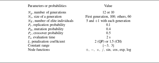

 Kij
 i
 j
 Jij

 a
 J
 b
 J
 j=1
 12
 c
 c

 a
 p′
 c
 q′/q∗′
 e
 B′
 b
 d
 f

 a
 q′
 p′
 Δθqp=θq−θp
 b
 PLV
 PLV≈1

 u′/u¯
 fg=(0.79±0.02)f1
 B′

 a
 t1
 t5
 b
 t6
 t10
 c
 λ∗
 λ
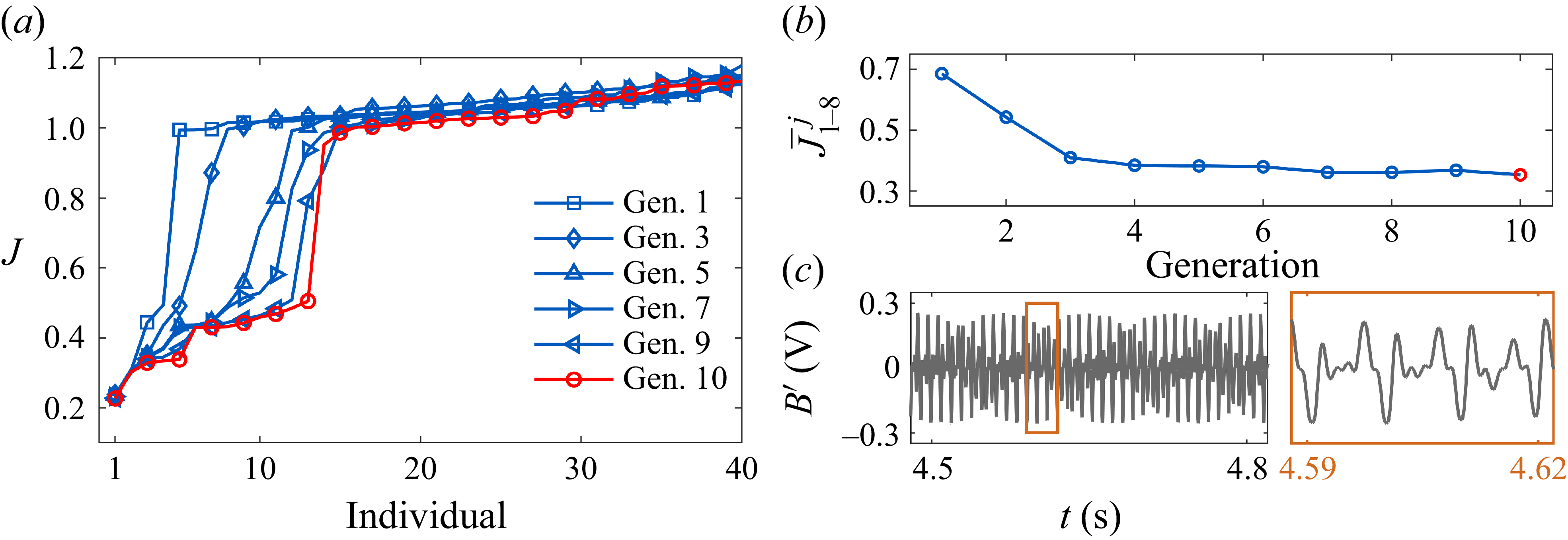
 a
 J
 b
 J
 j=1
 10
 c

 a
 ◯
 b
 △
 c
 ◻
 d
 KGCC
 KGOC
 KOLC
 J
 |η|
 Brms′
 e
 f
 g

 a
 J
 b
 J
 j=1
 10
 c
 c

 a
 p′
 d
 q′/qmax′
 g
 B′
 b,c
 e,f
 h,i

 q′
 p′
 Δθqp=θq−θp

 u′/u¯
 fg=(0.81±0.04)f1

 a
 t1
 t5
 b
 t6
 t10

 p′
 a
 mc,nc
 b
 20000
 2.0
 d=5
 c
 CJS
 H
 5000
 0.5
 d=6
 c
 CJS

 a
 J
 b
 J
 j=1
 10

 a
 ◯
 b
 △
 c
 ◻
 d
 KGCC
 KGOC
 KOLC
 J
 |η|
 Brms′
 e
 f
 g
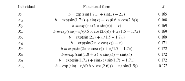

 x
 b
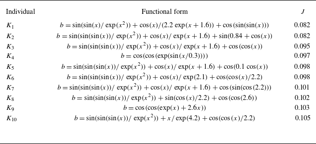

 x
 b

 f1
 f2
 f1−f2
 fg
 A~
 σ

 f1
 f2
 fg
 A~
 σ

 Open access

