





Introduction
To detect life in the Galaxy, a key issue is understanding where we should target our telescopic resources. For instance, in the search for technosignatures, observational resources should examine planets most likely to harbor intelligent life capable of producing technology (Enriquez et al., Reference Enriquez, Siemion, Foster, Gajjar, Hellbourg, Hickish, Isaacson, Price, Croft, DeBoer, Lebofsky, MacMahon and Werthimer2017; Gajjar et al., Reference Gajjar, Perez, Siemion, Foster, Brzycki, Chatterjee, Chen, Cordes, Croft, Czech, DeBoer, DeMarines, Drew, Gowanlock, Isaacson, Lacki, Lebofsky, MacMahon, Morrison and Pete Worden2021). Further, in the search for multicellular (versus microbial) life, we should use techniques to detect multicellular life on exoplanets versus techniques that detect only microbial life (Doughty and Wolf, Reference Doughty and Wolf2010; Doughty et al., Reference Doughty, Abraham, Windsor, Mommert, Gowanlock, Robinson and Trilling2020). Therefore, a means to estimate at what evolutionary stage a planet could be would provide a valuable constraint for telescope design and interpretation of observations. We propose a very simple hypothesis to address this issue:
The biological evolution rate is a linear function of cumulative carbon fixed on a planet.
In the absence of other information, estimating total potential carbon fixed or photosynthesis on exoplanets and comparing this to carbon fixed on Earth and its associated biological evolutionary stage can help estimate whether life on exoplanets found in the solar neighborhood are microbial, multicellular, or intelligent. Because Earth is currently the only known planet to harbor life, we cannot either prove or disprove this hypothesis, but we can explore its implications, which is the goal of this paper. We do not suggest more carbon fixed leads to “advancement” since unicellular organisms are already advanced by, for example, changing their metabolism in a way multicellular organisms cannot. Instead, we assume along the lines of the evolutionary speed hypothesis (ESH) presented in Gillman and Wright (Reference Gillman and Wright2014), which correlates speciation and species richness with genetic evolution. No “advancement” is included in this hypothesis, just species diversification.
We hypothesize that the biological evolutionary state is a linear function of genetic mutations which is a function of lives lived and is a function of cumulative carbon fixed (known in ecology as net primary production (NPP)) because in the absence of other information carbon fixed can be used as a rough estimate of the number of microbe/plant/animal lives lived (or genetic evolution). Assuming Darwinian evolution, a baseline astrobiological assumption (Des Marais et al., Reference Des Marais, Allamandola, Benner, Boss, Deamer, Falkowski, Farmer, Hedges, Jakosky, Knoll, Liskowsky, Meadows, Meyer, Pilcher, Nealson, Spormann, Trent, Turner, Woolf and Yorke2003), each generation of life has a small potential for genetic change following either sexual or asexual reproduction. These genetic changes will either be successful or not depending on the environment, species competition or predation around the organism. We therefore hypothesize that Earth’s cumulative carbon fixed at certain periods has led to major evolutionary transitions such as the emergence of photosynthetic organisms, eukaryote and multicellular animals that fundamentally altered the Earth’s carbon cycle, accelerating it at certain points. However, we acknowledge that this is an untestable hypothesis, and an alternate explanation is that these major carbon cycle altering events were not the result of Darwinian evolution based on mutations of genomic information but instead episodic events where higher order living systems emerged because of the integration of previously existing subsystems (Szathmáry and Smith, Reference Szathmáry and Smith1995). Moving forward, however, all calculations in the paper will be based on the cumulative fixed carbon hypothesis. For exoplanets, we have no information on such environmental changes or species compositions and without this knowledge, we propose that the biological evolutionary state is a function of genetic mutations which is a function of lives lived and is hence a function of carbon fixed.
Support for this argument for the importance of primary production (carbon fixed) for estimating biological evolutionary rates can be found by studying patterns of species richness and evolutionary rates on Earth. One of the most well-documented and theorized global patterns in biogeography is the latitudinal diversity gradient (LDG), in which taxonomic richness increases dramatically with decreasing latitude, being highest in the tropics near the equator (Gillman and Wright, Reference Gillman and Wright2014). Not only does the LDG exist today, but it has existed for at least 300 million years (Powell, Reference Powell2007), suggesting that it represents a generalizable pattern across geologic ages. Rohde (Reference Rohde1992), in a paper searching for the ultimate underlying causes of these patterns, suggested that species richness can be explained by differences in the rate of evolution multiplied by the amount of time there has been to accumulate them (Gillman and Wright, Reference Gillman and Wright2014; Rohde, Reference Rohde1992). Rohde placed high likely importance on temperature as a key driver of biological evolutionary rate via its influence on the speed of physiological processes, generation times and genetic mutation rate.
Others have shown that the presence of water strongly mediates this relationship, and that the relationships between both temperature and water and biological evolutionary rates may be due to their combined impact on vegetation productivity, a theory known as the integrated ESH (Gillman and Wright, Reference Gillman and Wright2014). Identifying productivity as central to evolutionary speed is supported by strong empirical relationships between productivity and species richness (Cusens et al., Reference Cusens, Wright, McBride and Gillman2012; Gillman and Wright, Reference Gillman and Wright2014; Kreft and Jetz, Reference Kreft and Jetz2007) and between productivity and evolutionary speed. Various taxa have been found to have faster evolutionary rates in warmer, more productive systems like low elevations (Bleiweiss, Reference Bleiweiss1998; Wright et al., Reference Wright, Gillman, Ross and Keeling2010) and in shallow ocean waters (Wright et al., Reference Wright, Ross, Jeanette Keeling, McBride and Gillman2011) relative to neighboring less productive areas (e.g. higher elevation or deeper in the ocean). While available solar energy is also often correlated with productivity, recent studies (see Honkanen et al., Reference Honkanen, Roberge, Rajasärkkä and Mönkkönen2010) have disentangled these covariates, finding “productive energy” (carbon sequestered; resources available to consumers) to be a better metric than solar energy input for predicting species richness (Honkanen et al., Reference Honkanen, Roberge, Rajasärkkä and Mönkkönen2010). In general, terrestrial ecosystem productivity can be limited by temperature, water availability, or light depending on the regional climate type (Nemani et al., Reference Nemani, Keeling, Hashimoto, Jolly, Piper, Tucker, Myneni and Running2003). Nutrient availability can also constrain the productivity of the ocean biosphere, specifically the availability of P, N and trace metal catalysts such as Fe, Ni and V (Bristow et al., Reference Bristow, Mohr, Ahmerkamp and Kuypers2017),
Models have been developed that estimate carbon fixed by plants and microbes. The Global Carbon Budget project (Friedlingstein et al., Reference Friedlingstein, O’Sullivan, Jones, Andrew, Bakker, Hauck, Landschützer, Le Quéré, Luijkx, Peters, Peters, Pongratz, Schwingshackl, Sitch, Canadell, Ciais, Jackson, Alin, Anthoni and Zheng2023) now annually reports estimates of the trends in Earth’s budget of carbon fluxes to the atmosphere and their uncertainties, summarized from observational data and multiple dynamic global vegetation and ocean biogeochemistry models (see their Table 4 for a list of the models). There are two models that assimilate remotely sensed indicators of photosynthetic activity, the Carnegie-Ames-Stanford approach (CASA) model for land and the Vertically Generalized Production Model for the oceans, which estimate that the modern-day total NPP of Earth is ∼104.9 Pg C yr-1, about evenly divided between terrestrial and marine sources (Field et al., Reference Field, Behrenfeld, Randerson and Falkowski1998). Global model estimates can range from complex Earth system models like NCAR’s community land model (CLM) (Oleson et al., Reference Oleson, Lawrence and Bonan2010) to simple empirical models like the Miami model (Lieth, Reference Lieth, Lieth and Whittaker1975). Such models suggest that global terrestrial NPP during the Carboniferous (359−299 Ma) was 33.7 Pg C yr-1 (Beerling et al., Reference Beerling, Woodward, Lomas, Wills, Quick and Valdes1998), of the same order of magnitude as a current value obtained from CASA (48 Pg C yr-1) and the range (44–57 Pg C yr-1) estimated by a more recent remote sensing-based model (Bloom et al., Reference Bloom, Exbrayat, van der Velde, Feng and Williams2016; Ciais et al., Reference Ciais, Yao, Gasser, Baccini, Wang, Lauerwald, Peng, Bastos, Li, Raymond, Canadell, Peters, Andres, Chang, Yue, Dolman, Haverd, Hartmann, Laruelle and Zhu2021; Crisp et al., Reference Crisp, Dolman, Tanhua, McKinley, Hauck, Bastos, Sitch, Eggleston and Aich2022), suggesting relatively stable global NPP once higher plants had evolved.
Total planetary NPP was probably lower prior to the evolution of oxygenic photosynthesis as anoxic microbes often have simple, less efficient photosynthesis and a recent empirical study showed anoxic microbial mats fixed about half the carbon as oxygenic mats under similar conditions (Ritchie et al., Reference Ritchie, Larkum and Ribas2018). Current research suggests that Earth is 4.5 billion years old, microbial life on Earth started as early as 3.7 billion years ago and possibly as early as 4.2 Gyr ago (Moody et al., Reference Moody, Álvarez-Carretero, Mahendrarajah, Clark, Betts, Dombrowski, Szánthó, Boyle, Daines, Chen, Lane, Yang, Shields, Szöllősi, Spang, Pisani, Williams, Lenton and Donoghue2024). There is biomarker evidence for simple sponges in the Cyrogenian (720–635 Ma) period (Love and Zumberge, Reference Love and Zumberge2021) but land plants did not appear until the late Ordovician and vascular plants didn’t diversify until the late Silurian-Early Devonian (418–407 Ma) (Gensel, Reference Gensel2008). Therefore, the start of life and the evolution of higher plants required roughly 3–3.5 billion years. We do not know whether higher plants on other planets would evolve after a similar amount of carbon fixed, but in the absence of other information we propose it as a reasonable hypothesis.
Recently there has been an explosion of interest in astrobiology because of the number of new exoplanet discoveries. At the time of writing there are ∼6,045 confirmed exoplanets (Christiansen et al., Reference Christiansen, McElroy, Harbut, Ciardi, Crane, Good, Hardegree-Ullman, Kesseli, Lund, Lynn, Muthiar, Nilsson, Oluyide, Papin, Rivera, Swain, Susemiehl, Tam, van Eyken and Beichman2025). Much attention has been focused on exoplanets that might harbor life and on methods to identify biosignatures on these planets. Identifying how photosynthesis might function on such planets has been a major area of research (Battistuzzi et al., Reference Battistuzzi, Cocola, Claudi, Pozzer, Segalla, Simionato, Morosinotto, Poletto and La Rocca2023; Eager-Nash et al., Reference Eager-Nash, Daines, McDermott, Andrews, Grain, Bishop, Rogers, Smith, Khalek, Boxer, Mak, Ridgway, Hébrard, Lambert, Lenton and Mayne2024; Kiang et al., Reference Kiang, Segura, Tinetti, Blankenship, Cohen, Siefert, Crisp and Meadows2007a, Reference Kiang, Siefert, Govindjee and Blankenship2007b; Lehmer et al., Reference Lehmer, Catling, Parenteau, Kiang and Hoehler2021; Ritchie et al., Reference Ritchie, Larkum and Ribas2018; Schwieterman et al., Reference Schwieterman, Kiang, Parenteau, Harman, Dassarma, Fisher, Arney, Hartnett, Reinhard, Olson, Meadows, Cockell, Walker, Grenfell, Hegde, Rugheimer, Hu and Lyons2018; Takizawa et al., Reference Takizawa, Minagawa, Tamura, Kusakabe and Narita2017). Most of the stars in our stellar neighborhood are red dwarf stars with a stellar spectral energy distribution shifted into the near infrared (NIR) relative to that of our sun. Oxygenic photosynthesis on Earth is limited to photosystems that operate at 400–750 nm (Chen, Reference Chen and Grimm BBT-A2019; Zhen and Bugbee, Reference Zhen and Bugbee2020) with inefficient use of photons up to as high as ∼780 nm (Pettai et al., Reference Pettai, Oja, Freiberg and Laisk2005), but anoxygenic photosynthesis occurs at wavelengths as long as 1015–1020 nm (Ritchie et al., Reference Ritchie, Larkum and Ribas2018; Trissl, Reference Trissl1993). Therefore, anoxic microbes fixing carbon at wavelengths up to 1100 nm (the shortwave (SW) cut-off for charge-coupled device detectors or “optical” wavelengths) could have an advantage in cooler red dwarf star systems over oxygenic photosynthetic organisms that can efficiently only use up to 750 nm (Catling et al., Reference Catling, Krissansen-Totton, Kiang, Crisp, Robinson, Dassarma, Rushby, Del Genio, Bains and Domagal-Goldman2018; Kiang et al., Reference Kiang, Siefert, Govindjee and Blankenship2007b; Ritchie et al., Reference Ritchie, Larkum and Ribas2018; Zhen et al., Reference Zhen and Bugbee2020). Ritchie et al., (Reference Ritchie, Larkum and Ribas2018) grew both anoxic and oxygenic photosynthetic mats under light conditions for a cool red dwarf (Proxima Centauri b) and found quite high rates of photosynthesis for both. However, it would be advantageous for photosynthetic organisms to be able to harvest the more abundant NIR light.
In this paper, we initially focus on TRAPPIST-1, a cool red dwarf star with seven known rocky exoplanets (Gillon et al., Reference Gillon, Triaud, Demory, Jehin, Agol, Deck, Lederer, de Wit, Burdanov, Ingalls, Bolmont, Leconte, Raymond, Selsis, Turbet, Barkaoui, Burgasser, Burleigh, Carey and Queloz2017), several of which are in the circumstellar habitable zone (Kasting and Catling, Reference Kasting and Catling2003; Kopparapu et al., Reference Kopparapu, Ramirez, Kasting, Eymet, Robinson, Mahadevan, Terrien, Domagal-Goldman, Meadows and Deshpande2013). It is targeted with current and future observatories (Lin et al., Reference Lin, MacDonald, Kaltenegger and Wilson2021; Lustig-Yaeger et al., Reference Lustig-Yaeger, Meadows and Lincowski2019; May et al., Reference May, Taylor, Komacek, Line and Parmentier2021; de Wit et al., Reference de Wit, Doyon, Rackham, Lim, Ducrot, Kreidberg, Benneke, Ribas, Berardo, Niraula, Iyer, Shapiro, Kostogryz, Witzke, Gillon, Agol, Meadows, Burgasser and Owen2024) that will give us further information about atmospheric composition and whether liquid water could be present on the surface. For instance, recent observations by the James Webb Space Telescope (JWST) suggest that TRAPPIST-1b may be an airless world (Greene et al., Reference Greene, Bell, Ducrot, Dyrek, Lagage and Fortney2023; Ih et al., Reference Ih, Kempton, Whittaker and Lessard2023), while TRAPPIST-1c may have no atmosphere or a thin O2-CO2 atmospheres atmosphere (Lincowski et al., Reference Lincowski, Meadows, Zieba, Kreidberg, Morley, Gillon, Selsis, Agol, Bolmont, Ducrot, Hu, Koll, Lyu, Mandell, Suissa and Tamburo2023; Zieba et al., Reference Zieba, Kreidberg, Ducrot, Gillon, Morley, Schaefer, Tamburo, Koll, Lyu, Acuña, Agol, Iyer, Hu, Lincowski, Meadows, Selsis, Bolmont, Mandell and Suissa2023). Models suggest that the outer planets of the TRAPPIST-1 system like TRAPPIST-1e (T1e) have significant water according to Gialluca et al. (Reference Gialluca, Barnes, Meadows, Garcia, Birky and Agol2024) although other models predict a complete loss of volatiles on TRAPPIST-1 planets (Van Looveren et al., Reference Van Looveren, Güdel, Boro Saikia and Kislyakova2024). T1e also is suggested to be tidally locked (e.g., Barnes et al., Reference Barnes2017) meaning that one face of the planet is constantly exposed to its host star (Barnes, Reference Barnes2017). Tle’s tidal locking implies that the substellar point (point of maximum stellar radiation) may have increased temperatures and provided as source of water, increased cloud cover (Yang et al., Reference Yang, Cowan and Abbot2013). Increased cloud cover increases albedo, thus cooling down the climate, delaying a moist greenhouse state (which is characterized by a H2O flux into the upper atmosphere and its subsequent loss due to photodissociation – see e.g., Badhan et al., Reference Badhan, Wolf, Kopparapu, Arney, Kempton, Deming and Domagal-Goldman2019).
Recently, an intercomparison of climate models for T1e has been carried out with four widely used exoplanetary general circulation models – ExoCAM, LMD-G, ROCKE-3D and the UM (Fauchez et al., Reference Fauchez, Turbet, Wolf, Boutle, Way, Del Genio, Mayne, Tsigaridis, Kopparapu, Yang, Forget, Mandell and Domagal Goldman2020; Sergeev et al., Reference Sergeev, Fauchez, Turbet, Boutle, Tsigaridis, Way, Wolf, Domagal-Goldman, Forget, Haqq-Misra, Kopparapu, Lambert, Manners and Mayne2022; Turbet et al., Reference Turbet, Fauchez, Sergeev, Boutle, Tsigaridis, Way, Wolf, Domagal-Goldman, Forget, Haqq-Misra, Kopparapu, Lambert, Manners, Mayne and Sohl2022). This project – The TRAPPIST-1 Habitable Atmosphere Intercomparison (THAI) – found reasonably close results of the four models for dry simulations (global mean surface temperature difference within 6–7 K for CO2 dominated atmosphere). Sergeev et al. (Reference Sergeev, Fauchez, Turbet, Boutle, Tsigaridis, Way, Wolf, Domagal-Goldman, Forget, Haqq-Misra, Kopparapu, Lambert, Manners and Mayne2022) compared climate simulations for T1e assuming a moist atmosphere dominated by either nitrogen or carbon dioxide and found global mean surface temperature varied between these two scenarios by 14 and 24 K respectively. They found some important intermodal differences in various climate diagnostics amplified by approximations used in the parameterizations of moist physics such as cloud formation, with ExoCAM producing the warmest climate and UM the coolest.
In this paper, we explore the implications of the hypothesis that biological evolutionary state is a function of total potential carbon fixed using climate maps from the THAI study (Fauchez et al., Reference Fauchez, Turbet, Wolf, Boutle, Way, Del Genio, Mayne, Tsigaridis, Kopparapu, Yang, Forget, Mandell and Domagal Goldman2020; Sergeev et al., Reference Sergeev, Fauchez, Turbet, Boutle, Tsigaridis, Way, Wolf, Domagal-Goldman, Forget, Haqq-Misra, Kopparapu, Lambert, Manners and Mayne2022; Turbet et al., Reference Turbet, Fauchez, Sergeev, Boutle, Tsigaridis, Way, Wolf, Domagal-Goldman, Forget, Haqq-Misra, Kopparapu, Lambert, Manners, Mayne and Sohl2022). We calculate total carbon fixed on Earth over time and across different biological evolutionary stages such as microbial and higher plant life. Then we estimate how long other planets would have taken to achieve the same amount of carbon fixed. We start with climate simulations of T1e, an older planet than Earth at ∼7.6 ± 2.2 billion years (Burgasser and Mamajek, Reference Burgasser and Mamajek2017), with spatially explicit maps of temperature, irradiance, precipitation and cloud cover. Then we use data from the habitable worlds catalog (https://phl.upr.edu/hwc) to estimate NPP and evolutionary stage for the 29 planets currently most likely candidates to harbor life. We explore the following questions:
Q1 – If biological evolution is a linear function of carbon fixed, would T1e, an older planet with a lower solar flux and less surface area, be less or more advanced than the biological evolutionary stage on Earth?
Q2 – Would any of the exoplanets within the Solar Neighborhood be more advanced than Earth in terms of biological evolution?
Methods
T1e climate and NPP
We used simulated climatology data for T1e from the THAI experiment (Fauchez et al., Reference Fauchez, Turbet, Wolf, Boutle, Way, Del Genio, Mayne, Tsigaridis, Kopparapu, Yang, Forget, Mandell and Domagal Goldman2020, Reference Fauchez, Turbet, Sergeev, Mayne, Spiga, Sohl, Saxena, Deitrick, Gilli, Domagal-Goldman, Forget, Consentino, Barnes, Haqq-Misra, Way, Wolf, Olson, Crouse, Janin and Bouldin2021) as well as GCM simulated modern Earth climatology to estimate surface productivity for different atmosphere and surface composition scenarios. For most results, we used the Met Office Unified Model (UM) model (Mayne et al., Reference Mayne, Baraffe, Acreman, Smith, Wood, Amundsen, Thuburn and Jackson2014) simulations (144 longitudes by 90 latitudes) of the downwelling SW solar flux at surface (FSWdown), time-average precipitation flux and surface temperature (TS) (downloaded on June 1, 2024 – Fauchez et al., Reference Fauchez, Turbet, Sergeev, Mayne, Spiga, Sohl, Saxena, Deitrick, Gilli, Domagal-Goldman, Forget, Consentino, Barnes, Haqq-Misra, Way, Wolf, Olson, Crouse, Janin and Bouldin2021). We also compared these results to simulations from ExoCAM (Exoplanet Community Atmosphere Model – derived from the CAM4 NCAR model). For most results, we used Hab 1 simulations of a single layer slab ocean covered planet with 400 ppm CO2, but we also employed Hab 2 simulations which have an atmosphere of 1 bar of CO2 averaged over 100 TRAPPIST-1e orbits. We used two models, UM and ExoCAM, because they represent the endmembers of the THAI models in terms of planetary temperatures with ExoCAM producing the warmest climate and UM the coolest (Sergeev et al., Reference Sergeev, Fauchez, Turbet, Boutle, Tsigaridis, Way, Wolf, Domagal-Goldman, Forget, Haqq-Misra, Kopparapu, Lambert, Manners and Mayne2022). For Earth simulations, we used NCAR’s CLM 4.0 (Oleson et al., Reference Oleson, Lawrence and Bonan2010) monthly data averaged over 12 months (288 longitudes by 192 latitudes) for atmospheric incident solar radiation (diagnostic name FSDS), 2-m air temperature (TSA) and atmospheric precipitation (RAIN). We specifically ran the model using compset F_2000_CN with details in Doughty et al. (Reference Doughty, Santos-Andrade, Shenkin, Goldsmith, Bentley, Blonder, Díaz, Salinas, Enquist, Martin, Asner and Malhi2018).
We used simulated climatologies of stellar radiation, temperature and precipitation for both T1e and Earth to calculate NPP with the Miami model (Lieth, Reference Lieth, Lieth and Whittaker1975) For each grid cell of the above datasets, we used the Miami model Equations (1)–(4) below to estimate NPP in units of grams of dry matter m-2 yr-1 as limited by temperature and precipitation on land and temperature and nutrients in the ocean. We have added a simple function (Equation (3)) for nutrient limitation in the ocean, which was not included in the original Miami model. Ocean NPP starts with a maximum of 500 g m-2 yr-1 in nutrient rich waters to <10 g m-2 yr-1 in low nutrient waters (Boyd et al., Reference Boyd, Sundby, Pörtner, Field, Barros, Dokken, Mach, Mastrandrea, Bilir, Chatterjee, Ebi, Estrada, Genova, Girma, Kissel, Levy, MacCracken, Mastrandrea and White2014).
 $${\rm{NP}}{{\rm{P}}_{\rm{T}}} = 3000{ ^*}(1 + {\rm{exp}}(1.315 - 0.119{ ^*}{\rm T})){\;^ \wedge }^{ - 1}$$
 $${\rm{NP{P_T}}} = 3000{ ^*}(1 + {\rm exp}{(1.315 - 0.119{ ^*}({\rm T} - {2^*}{\rm{(T - threshold)))}}^ \wedge }^{ - 1}$$
 $${\rm NP{P_P}}{\rm{ = }}3000{ ^{\rm{*}}}(1 - {\rm exp}({\rm{ - }}0.00066 {4^{\rm{*}}}{\rm P}))$$
 $${\rm NPP_N = 500 \, ^*(1 - exp(-0.2 \, ^* N))}$$
 $${\rm NPP_{final\_land} = min(NPP_T,\, NPP_P)_{land}}$$
 $${\rm NPP_{final\_ocean} = min(NPP_T,\, NPP_N)_{oceans}}$$
where T is temperature (°C), P is precipitation (mm/yr), N is nitrate (μmol l-1), NPPT is the NPP response to temperature, NPPP is the response to precipitation and NPPN is the response to nutrients. In a sensitivity study, we use Equation (1b) to add an upper temperature threshold of 35°C, 40°C, 45°C with its effect on NPPT under these three scenarios shown in Figure S1a. The Miami model does not incorporate light limitation on NPP; however, light is critical for photosynthesis. To incorporate radiation levels into our NPP estimates, we used maps of downwelling stellar flux at the surface in W m-2 (FSWdown) and Equations (5) for NPP 400–700 nm and 6 for NPP 400–1100 nm. NPPfinal from Equation (3) for each point (i,j indicate column and row position on a 2d map) is scaled by the grid point’s incident photosynthetically active radiation (IPAR) relative to the Earth average in the spectral ranges of either 400–700 nm (Equation (5)) or 400–1100 nm (Equation (6)).
 $${\rm NPPland\,_{400-700 nm} = NPP_{final\_land}(i,j) ^*( F_{SW}\, ^{down} (i,j) /158)^* (1.5/11) \, ^*((S_p \,^*1361)/1135)}$$
 $$\small{\rm NPPocean\, _{400-700\, nm} = NPP_{final\_ocean}(i,j)\, ^*( F_{SW}\,^{down} (i,j) /158)^*(1.4^*0.95 + 1.1^*0.05)/11)\, ^*((S_p\, ^*1361)/1135)}$$
 $${\rm NPPland \,_{400-1100 \,nm} = NPP_{final\_land}(i,j)\, ^*( F_{SW}\,^{down} (i,j) /158)^* (16.9/11) \,^*((S_p \,^*1361)/1135)}$$
 $$\small{{\rm NPPocean \,_{400-1100 nm} = NPP_{final\_ocean}(i,j) \,^*( F_{SW}\,^{down} (i,j) /158)^*( 9.9^*0.95 + 1.5^*0.05)/11) \,^*((S_p \,^*1361)/1135)}}$$
Light on T1e has a different stellar spectrum and spectral flux compared to our Sun-Earth, so we then converted FSDS to planet-specific IPAR. We divide this by 158 because on Earth, the map of FSDS has an average of 158 W m-2, and dividing each pixel’s FSDS first by 158 W m-2 will normalize the surface light flux by the amount used in Earth’s NPP calculations. T1e light is a multiplier where, if light levels are greater than Earth’s FSDS average, NPP will increase linearly, and if less it will decrease linearly (we vary this assumption in a sensitivity study).
For the terrestrial part (NPPland) of the planet, we next multiply by 1.5/11 (Equation (5)) and 16.9/11 (Equation (6))) to scale the estimated photon flux density for planets relative to Earth (Kiang et al., Reference Kiang, Siefert, Govindjee and Blankenship2007a). Planetary continental cover fraction would be 0.3 like Earth or 0 for an ocean world. A cloudless Earth has a solar noon photosynthetic photon flux density (PPFD) of 11•1020 photons m-2 s-1 for 400–700 nm and we compare this to the simulated M5V planet (for low O2) which had a PPFD for 400–700 nm of 1.5•1020 photons m-2 s-1 for terrestrial surfaces. Using light from 400–1100 nm, the M5V planet has PPFD1100 of 16.9•1020 photons m-2 s-1for terrestrial surfaces. For instance, in Equations (5) and (6), we estimated that a M5V planet in the terrestrial regions will have a ratio of 1.5/11 or 14% of the usable light as Earth between 400 and 700 nm and 17/11 or 150% of the usable light as Earth between 400–1100 nm. Due to high uncertainty, we varied these numbers by 20% in a sensitivity study.
There are clearly no precipitation limitations in the ocean, but productivity in most of the ocean on Earth (∼75%) is limited by nutrients such as inorganic nitrogen (Bristow et al., Reference Bristow, Mohr, Ahmerkamp and Kuypers2017). Therefore, for ocean regions (NPPocean), we assigned a nutrient limitation (N) with either a low 1 (75% of ocean pixels) or high 30 μmol l-1 (25%) nitrate concentration (Bristow et al., Reference Bristow, Mohr, Ahmerkamp and Kuypers2017). Nitrate limitations will reduce peak NPP through a simple exponential decay function (Equation (3)) shown in Figure S1b and varied in a sensitivity study. Most oceanic photosynthesis is in the photic zone which is typically the top 100 m. We assume 95% of the ocean photosynthesis will be below the top 0.1 m of the surface. Light in the red and near-infrared does not transmit well through water, and we approximated the ocean photon flux for 400–700 nm (Equation (5)) as a weighted average of 5% water at 5 cm with 1.4•1020 photons m-2 s-1 and 95% at 100 cm with 1.1•1020 photons m-2 s-1 (varied in a sensitivity study). For 400–1100 nm (Equation (6)) we used 5% water at 5 cm with 9.9•1020 photons m-2 s-1 and 95% at 100 cm with 1.5•1020 photons m-2 s-1. Therefore, for the marine part of the planet (∼70%), we next multiply by (((1.4*0.95 + 1.1*0.05))/11) ((Equation (5)) and (((9.9*0.95 + 1.5*0.05))/11) (Equation (6)).
We then scaled this value, which is valid for the M5V planet to T1e and other exoplanets with the final part of the equation: ((Sp *1361)/1135). The top of atmosphere stellar flux for the M5V planet in Kiang et al. (Reference Kiang, Siefert, Govindjee and Blankenship2007b) was 1135 W/m2. The top-of-atmosphere simulated Earth solar constant is 1361 W/m2 (Prša et al., Reference Prša, Harmanec, Torres, Mamajek, Asplund, Capitaine, Christensen-Dalsgaard, Depagne, Haberreiter, Hekker, Hilton, Kopp, Kostov, Kurtz, Laskar, Mason, Milone, Montgomery, Richards and Stewart2016). In our equation, we used the ratio of the planet solar flux relative to Earth, Sp relative to the M5V planet in Kiang et al. (Reference Kiang, Siefert, Govindjee and Blankenship2007b). For instance, TRAPPIST-1e has a solar flux ratio to Earth of Sp = 0.65 (Agol et al., Reference Agol, Dorn, Grimm, Turbet, Ducrot, Delrez, Gillon, Demory, Burdanov, Barkaoui, Benkhaldoun, Bolmont, Burgasser, Carey, de Wit, Fabrycky, Foreman-Mackey, Haldemann, Hernandez, Ingalls, Jehin, Langford, Leconte, Lederer, Luger, Malhotra, Meadows, Morris, Pozuelos, Queloz, Raymond, Selsis, Sestovic, Triaud and Grootel2021), such that T1e is 65% of 1361 W m-2, or 885 W m-2. Therefore, T1e NPP was scaled by 885/1135 or a ratio of 0.78 to the generic M5V planet.
We quantified light-, temperature-, and precipitation-limited regions on Earth and on exoplanets following (Nemani et al., Reference Nemani, Keeling, Hashimoto, Jolly, Piper, Tucker, Myneni and Running2003) in Equation (7).
 $$\eqalign{ & {\rm{ - }}{\rm{if\;T \gt 15\; P \gt 1500 \;{F_{SW}}{ ^{down}} \lt 200\;W {m^{ - 2}}\;then\;Ligh{t_{lim}}}} \cr & {\rm{elseif\;NP{P_T} \gt NP{P_P}\;then\;Preci{p_{lim}}}} \cr & {\rm{else\;Tem{p_{lim}}}} \cr}$$
In Equation (7), where T is temperature (°C) and P is precipitation (mm/yr), we show whether each pixel is light, temperature or precipitation limited (respectively, logical, Lightlim, Preciplim, Templim). We used Equation (3) from the Miami model to determine temperature- and precipitation-limited regions, but employed the approach of Nemani et al. (Reference Nemani, Keeling, Hashimoto, Jolly, Piper, Tucker, Myneni and Running2003) to estimate that warm wet regions with high cloud cover are light limited. For Earth, from the CLM we determined light limited regions have surface temperature T > 15 Celsius, precipitation P > 1500 mm yr-1, and cloud cover >60%, roughly following Nemani et al. (Reference Nemani, Keeling, Hashimoto, Jolly, Piper, Tucker, Myneni and Running2003). For exoplanets, instead of cloud cover, we used a light threshold of 200 W m-2. We assume a terrestrial surface for each pixel for this analysis because we have no data for ocean nutrient limitations.
T1e evolutionary stage
We then summed total planetary NPP for both Earth and T1e in Pg C yr-1. The dataset for the CLM Earth simulation from Doughty et al., Reference Doughty, Santos-Andrade, Shenkin, Goldsmith, Bentley, Blonder, Díaz, Salinas, Enquist, Martin, Asner and Malhi2018 is just for land and we estimate current terrestrial NPP on Earth to be ∼53 Pg C yr-1which is close to more complex models like CASA (Field et al., Reference Field, Behrenfeld, Randerson and Falkowski1998) which estimate the annual terrestrial NPP at 56.4 Pg C yr-1. Cfrac above is to estimate continental fraction on exoplanets. On Earth we multiply the average per area NPP by the total surface area of the Earth which is 5.1 × 10¹⁴ m2. On T1e, we calculate the surface area based on the planetary radius.
We then compare the summed NPP for this period on Earth and then estimate the time it would require T1e to match this (Table 1 lists these values for each evolutionary stage). The first evidence for life on Earth dates to ∼3.7 billion years ago and then terrestrial/vascular plants evolved ∼500 million years ago (400 to 600 MYA in a sensitivity study – Table 2), and therefore microbial photosynthesis dominated Earth for 3 billion years (William Schopf, Reference William Schopf2011). We calculate Earth’s NPP for the first 3 billion years at a lower photosynthetic efficiency than current. Most photosynthesis does not occur in ideal conditions. For the Archean Ocean, ocean NPP could have been up to 40 times lower than the current ocean due to reductant limitations (Kharecha et al., Reference Kharecha, Kasting and Siefert2005) and the Proterozoic Ocean was likely 10% of modern oceans NPP due to lower nutrient recycling, among other reasons (Laakso and Schrag, Reference Laakso and Schrag2019). Continental ratio would also have varied from almost a water world during the Archean to a lower continental ratio during the Proterozoic. To incorporate the gradual increase in productivity from the Archean to the Phanerozoic, we use an efficiency of 0.025 for the first 1 Gyr (Archean) and 0.1 for the next 2 Gyr (Proterozoic). After the first three billion years, if an exoplanet was still at the microbial life stage, we set the photosynthetic efficiency to 0.47 based on average ideal photosynthesis rates between anoxic and oxygenic photosynthesis (Ritchie et al., Reference Ritchie, Larkum and Ribas2018).
Earth’s evolutionary stages: (1) microbial, (2) terrestrial/vascular plants and (3) the biological evolution of an intelligent species have the below estimated NPP values (Pg C/year) and cumulative organic carbon fixed (g C) for each stage

Table 1. Long description
A table comparing Earth’s evolutionary stages, estimated NPP values, and cumulative organic carbon fixed. The table has three columns and four rows, including the header row. The columns are labeled as Earth’s evolutionary stages, Estimated NPP values (Pg C/year), and Cumulative organic carbon fixed (g C). The rows detail the information for each evolutionary stage. Row 1: Earth’s evolutionary stages 1: microbial started on Earth ~3.7 billion years, Estimated NPP values 2.5 Pg C/year during the ~1 G year Archean and 10 Pg C/year during the ~2 G year of the Proterozoic, Cumulative organic carbon fixed 2.4 e25 g C. Row 2: Earth’s evolutionary stages 2: terrestrial/vascular plants started on Earth ~500 million years ago, Estimated NPP values 101 Pg C/year, Cumulative organic carbon fixed 7 e25 g C. Row 3: Earth’s evolutionary stages 3: the biological evolution of an intelligent species started on Earth ~200,000 years ago, Estimated NPP values 101 Pg C/year, Cumulative organic carbon fixed 9.4 e25 g C.
A sensitivity study where we vary our model coefficients to a low and high estimate from our best estimate (in bold). We change the multiplier of age when multicellularity arose, the estimated age of TRAPPIST-1e (TRAPPIST-1e age), the Miami model temperature multiplier (Miami T), the Miami model precipitation multiplier (Miami P), the radius of T1e as compared with Earth (Trap radius), the M5V/Earth light ratio from Equation (4)/(5) (i.e. 1.5/11 ± 20% and 17/11 ± 20%), and a multiplier for TRAPPIST-1e planetary temperature (Heat multiplier). We show <700 nm (red line from Figure 3) and <1100 nm (cyan line from Figure 3). Numbers estimate how far behind current day Earth is TRAPPIST-1e in billions of years (negative numbers are ahead and positive are behind) for the given scenario

Table 2. Long description
A table comparing various model coefficients and their impact on TRAPPIST-1e’s evolutionary timeline. The table has 10 rows and 8 columns. The columns are labeled as follows: Evo of multicellular life (600, 500, 400 MYA), TRAPPIST-1e age (9.8, 7.6, 5.4), Miami T (0.05 0.119 0.2), Miami P (-0.004 -0.000664 -0.001), Trap radius (1.1 0.92 0.7), M5V/Earth light ratio (0.14/1.5 ± 20%), and Heat multiplier (1.15 1 0.95). The rows are labeled as follows: <1100 nm and <700 nm. The values in the table are as follows: Row 1: <1100 nm, 10/17 Gy, 13/17 Gy, 14/15 Gy, 12/22 Gy, 9/30 Gy, 13/17 Gy, 15/24 Gy. Row 2: <700 nm, 96/142 Gy, 127/132 Gy, 120/128 Gy, 103/172 Gy, 89/227 Gy, 120/140 Gy, 130/187 Gy.
If T1e matches the summed carbon fixed during the first 3 billion years of anoxgenic photosynthesis, it can move to higher efficiency photosynthesis (e.g. Equation (6)). We then calculate higher efficiency photosynthesis (i.e. the standard Miami model without the Archean or Proterozoic multiplier). We then calculate how long each exoplanet requires to match Earth’s photosynthesis at the higher efficiency rate. We account for T1e’s estimated age (7.8 billion years) with the assumption that life originated close to the start of the planet’s history like Earth when calculating total carbon fixed and comparing it to Earth. If the summed carbon fixed for T1emicrobial exceeds that of Earth, we define it as multicellular (Equation (8)). We recognize that Earth had multicellular life as early as 700 million years ago, well before terrestrial/vascular plants evolved. However, for this paper we are making a simplifying assumption and using a similar time for both. If the summed carbon fixed for T1emicrobial + T1emulticellular exceeds that of Earth (Equation (9)), we define it as intelligent. By intelligent, we mean surpassing the cumulative NPP on Earth when modern humans evolved.
 $${\rm{ = }}{\rm{\,if (\sum {NPP} { _{400 - 1100\;nm}} Eart{h_{microbial}}\; \lt \;\sum {NPP} {\rm{ }}{ _{400 - 1100\;nm}}T1{e_{microbial}}) then \;T1e\; is\; multicellular}}$$
 $$\eqalign{ & {\rm{ = }}{\rm{\,if ({\sum {NPP} _{400 - 1100\;nm}} Eart{h_{microbial}}{\rm{ + }}\sum {NPP} { _{400 - 1100\;nm}}Eart{h_{multicellular}})\; \lt (\sum {NPP} }} _{400 - 1100\;nm} \cr & {\rm{T1{e_{microbial}}\; + \;{\sum {NPP} _{400 - 1100\;nm}}T1{e_{multicellular}}) then \;T1e\; is\;intelligent}} \cr}$$
Other planets evolutionary stage
We then used NASA data (https://exoplanetarchive.ipac.caltech.edu/) organized in the Habitable Worlds Catalog (https://phl.upr.edu/hwc) which has compiled a list of 29 Earth sized rocky planets (i.e., 0.5 < Planet Radius ≤ 1.6 Earth radii or 0.1 < Planet Minimum Mass ≤ 3 Earth masses) within the habitable zone of their host stars. This list has data on potential planet radius, irradiation, temperature, age and distance (Table 2). Since all the planets listed (except 2) orbit class M red dwarf stars, we use the stellar radiation, temperature and precipitation maps as a baseline for all planets. We then scale the stellar flux for each planet using the estimate of stellar radiation (Sp from Table 3 and Equation (5)) from the Habitable Worlds Catalog (i.e. by (Sp *1361)/1135 from Equation (5)). We use the top-of-atmosphere irradiance as an estimate of clear-sky surface irradiance, neglecting planet to planet changes in atmospheric absorbance. For example, for each pixel we will take surface downwelling irradiance and weight it by the following function from Equation (5): (Sp *1361)/1135. We then calculate the cumulative NPP fixed for each of these 29 planets and compare this to Earth’s NPP at each evolutionary stage. For example, if the exoplanet has less than Earth’s cumulative NPP from 500 million years ago we classify life stage as microbial, if it has Earth NPP > Earth from 500 million years ago but less than Earth current day (Equation (8)), we classify life stage as multicellular, if it has > Earth’s cumulative NPP from today we classify life stage as intelligent (Equation (9)). G-type stars, like the sun, have luminosities that have evolved significantly over geologic time, causing a long-term decline in CO2 concentration (Bahcall et al., Reference Bahcall, Pinsonneault and Basu2001) (Oosterloo et al., Reference Oosterloo, Höning, Kamp and van der Tak2021). However, the productivity of Earth intrinsically includes this long-term decline because the lower solar luminosity affected Earth´s NPP at a given time in the past. Further, this study is mainly about M dwarf stars that are more stable over long periods than G-type stars and would not experience similar long-term decline in CO2 concentrations (Ribas, Reference Ribas2009).
List of planets from habitable world’s catalog (https://phl.upr.edu/hwc) and their parameters ranked from highest to lowest according to Earth similarity index (ESI). We show planet radius compared to Earth, solar flux compared to Earth, temperature (K), estimated age of planet (if unknown 4. 5BY is assumed), distance to Earth in light years, time to pass Earth (GY) at HAB1 with <1100 nm and <700 nm light and ratio of Earth’s NPP. The last six columns are predicted life stage (1 = microbial (NPPexo < Earth-500 mya), 2 = multicellular (NPPexo > Earth-500 mya), 3 = intelligent (NPPexo > current Earth)) for <1100 nm light HAB1 planet with 30% continent with the UM model (te), <700 nm light HAB1 planet with 30% continent (te_700), <1100 nm light HAB1 planet with 0% continent (oc), and <1100 nm light HAB2 planet with 30% continent (H2_11), and <700 nm light HAB2 planet with 30% continent (H2_7)

Table 3. Long description
List of planets from habitable world’s catalog (https://phl.upr.edu/hwc) and their parameters ranked from highest to lowest according to Earth similarity index (ESI). We show planet radius compared to Earth, solar flux compared to Earth, temperature (K), estimated age of planet (if unknown 4.5BY is assumed), distance to Earth in light years, time to pass Earth (GY) at HAB1 with <1100nm and <700nm light and ratio of Earth’s NPP. The last six columns are predicted life stage (1=microbial (NPPexo< Earth-500 mya), 2= multicellular (NPPexo> Earth-500 mya), 3 = intelligent (NPPexo>current Earth)) for <1100nm light HAB1 planet with 30% continent with the UM model (te), <700nm light HAB1 planet with 30% continent (te_700), <1100nm light HAB1 planet with 0% continent (oc), and <1100nm light HAB2 planet with 30% continent (H2_11), and <700nm light HAB2 planet with 30% continent (H2_7).
Results
T1e NPP and evolutionary stage
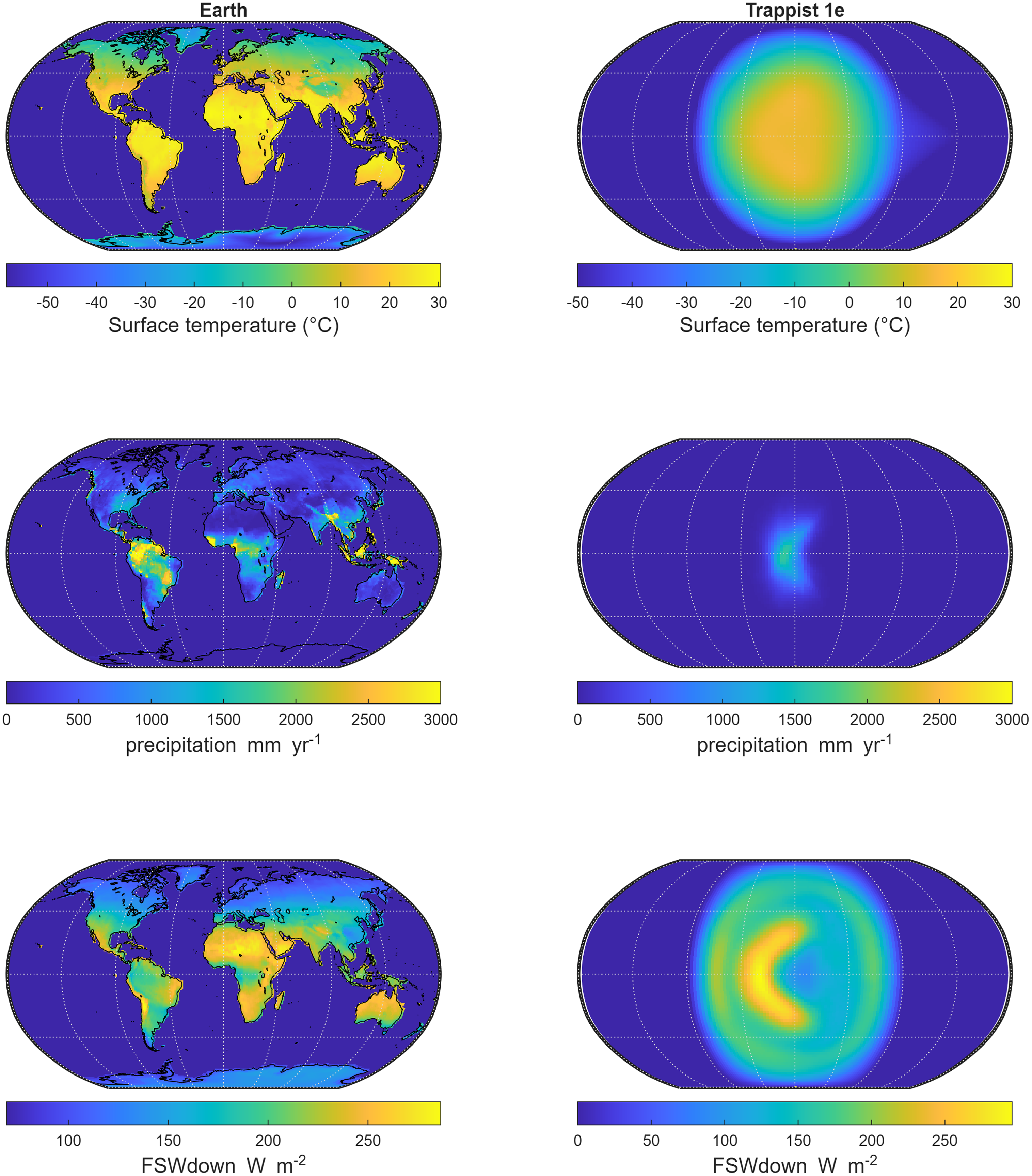
Shortwave radiation, temperature and precipitation show distinctly different patterns on T1e as an ocean world with 400 ppmv CO2 (Hab 1 and 2 from UM (Figure S2) and ExoCAM (Figure S2) than on Earth (from CLM) because in our simulations T1e is a tidally locked planet with a strong day–night contrast (Figure 1). The maximum average surface temperature on Earth (∼30°C) is generally higher than Hab 1 but similar to Hab 2 compared to that on T1e (∼15/36/22°C for UM Hab 1 & 2, ExoCAM Hab1, respectively; see Figures S2). The precipitation is concentrated in the substellar region on the day side of the planet (see e.g., Sergeev et al., Reference Sergeev, Lambert, Mayne, Boutle, Manners and Kohary2020 for more discussion) (Sergeev et al., Reference Sergeev, Lambert, Mayne, Boutle, Manners and Kohary2020). Global average precipitation is similar to Earth (439 mm yr-1) compared with Hab 2 but much greater than Hab 1 on T1e (26/582 mm yr-1 for UM Hab1/2 – there is no ExoCAM precipitation data available). As a result of higher temperatures, via the Clausius-Clapeyron relation, precipitation was greater for Hab 2(10,000 mm yr-1) versus for Hab 1 (10,000 mm yr-1). Maximum surface irradiance is similar at the center of the day side of T1e as compared to that on Earth for Hab1/2 but lower than ExoCam (∼286/296/292/386 W m-2 for Earth/UM Hab1/2/Exo Hab1, but its global average is lower (158/63/47/62 W m-2).
Surface temperature (deg C) (top), precipitation (mm yr-1) (middle), and downwelling shortwave radiation flux at surface W m-2 (bottom) for Earth (left) and T1e (right). The Earth estimates are taken from CLM 4.0. The data for T1e is from the THAI Hab 1 experiment (Sergeev et al., Reference Sergeev, Fauchez, Turbet, Boutle, Tsigaridis, Way, Wolf, Domagal-Goldman, Forget, Haqq-Misra, Kopparapu, Lambert, Manners and Mayne2022).
Using maps from Figure 1 and the Miami model Equations (1)–(6), we calculate global terrestrial NPP with Earth’s NPP highest in the tropical regions (<30 latitude) (Figure 2a) and most T1e Hab 1 NPP in the warm, wet, irradiated substellar region (Figure 2b). We do not know which wavelengths of light photosynthesis on T1e would use and we therefore calculate NPP for: (1) Hab 1 UM using wavelengths <1100 nm, (2) Hab 1 UM using <700 nm, (3) Hab 2 using wavelengths <1100 nm and (4) Hab 1 ExoCam using wavelengths <1100 nm (results shown in parentheses). Earth had a peak NPP of 1300 g C m-2 yr-1 which was similar to T1e for the scenarios using light <1100 nm (1260/126/2010/1730 g C m-2 yr-1) but much higher if only <700 nm were used. However, T1e was generally drier and darker than Earth with, for example, 62% of the surface area with 0 NPP in the UM Hab 1 case for T1e due to the absence of precipitation on continental regions or the absence of light on the non-illuminated regions. Therefore, Earth’s total annual NPP was much higher 101 Pg C yr-1 versus T1e (∼17/3/59/26 Pg C yr-1) for multicellular scenarios except for the Hab2 scenario which was closer due to increased precipitation. UM climates produced lower total NPP than ExoCam (17 vs 26 Pg C yr-1) due to the climate being colder (15°C max vs 22°C). The reduced T1e values reflect the smaller surface area overall, only half of which is illuminated and lower precipitation. For simplicity, we assume a random continental distribution on T1e amounting to 30% land, 70% ocean, but an ocean world would be less productive (because NIR light dominates on T1e but does not penetrate into water) with a total NPP of ∼4 Pg C yr-1 for UM Hab1 < 1100 nm.
Estimate of NPP on Earth (a) and TRAPPIST-1e HAB1 <700 nm (b), TRAPPIST-1e HAB1 <1100 nm (c), and TRAPPIST-1e HAB2 <700 nm (d) NPP in g m-2 yr-1 using the Miami model. For TRAPPIST-1e we randomly assign 30% as continental area.

Anoxic photosynthesis is less efficient than oxygenic photosynthesis and we estimate a microbial dominated world on Earth would fix 2.5 Pg C yr-1 during the ∼1 Gyr Archean and 10 Pg C yr-1 during the ∼2 Gyr of the Proterozoic, for a total carbon fixed for 3 billion years of 2.5 1025 g C fixed before the biological evolution of terrestrial/vascular plants. Earth had terrestrial/vascular plants for 500 million years (varied 400 to 600 Myr ago in a sensitivity study – Table 2) before the biological evolution of an intelligent species (humans) and we estimate that terrestrial/vascular plants fixed 101 Pg C yr-1 for ∼500 million years for a total of 7 e25 g C (i.e. 1/4 cumulative NPP is microbial and 3/4 is terrestrial/vascular plants). Therefore, we estimate Earth has fixed a total of ∼9.4 e25 g C until now. T1e Hab 1 fixed 2.5 1025 (the amount of carbon fixed by Earth during the 3 Gyr microbial stage) at the lower anoxic photosynthesis rate after ∼9/36/3/6 Gyr at which point it evolves terrestrial/vascular plants which photosynthesize more efficiently (Figure 3). T1e then fixed cumulatively ∼9.4 e25 C (Earth’s cumulative carbon fixed) after ∼17/84/7/11 Gyr. Since TRAPPIST-1e is estimated to be 7.6 billion years old (Burgasser and Mamajek, Reference Burgasser and Mamajek2017), or 3 Gyr older than Earth, we estimate its biosphere (if it exists) to be 14 Gyr years behind ours in evolutionary terms and still at the microbial life stage for the UM Hab 1 < 1100 nm. However, the UM Hab 2 < 1100 nm may be slightly ahead of us, while if photosynthetic life on T1e evolved to only use <700 nm of light, then we estimate it is far behind us. In our NPP model, T1e Hab 1 was precipitation limited (meaning more precipitation will always increase NPP) while the substellar region in the T1e Hab 2 scenario was temperature limited (Figure 4). Compare this to Earth, where most of NPP is precipitation limited (Figure 4).
Total NPP produced over time for the HAB1 simulation for T1e under four scenarios: use of light <700 light (red line), use of light <1100 nm with 30% terrestrial, 70% ocean (cyan line), use of light <1100 nm with 100% ocean (blue line), and use of light <1100 nm with 30% terrestrial and Hab2 climate (green line). We assume life on T1e started quickly like on Earth. The vertical yellow line shows 7.8 billion years which is the current estimate of the age of T1e. The horizontal black line is our estimate of total carbon fixed thus far by Earth.

NPP limitations according to Equation (7) for continental areas on Earth (top), T1e Hab1 (middle), and T1e Hab2 (bottom) showing whether an addition of light temperature or precipitation would lead to more NPP. This calculation is assuming a terrestrial surface for each pixel.

Sensitivity study
A sensitivity study (see details in Table 2) suggests that our model coefficients for a UM HAB1 T1e climate would affect our quantitative predictions but not enough to change the estimated evolutionary stage (i.e. microbial/multicellular/intelligent). In other words, we changed seven main parameters by a ∼ standard deviation (when available), but all simulations for Hab 1 T1e remained in the microbial life stage under our most likely scenario (Hab1 and <1100 nm light). Changes between the high and low values for the other parameters like temperature and precipitation from the Miami model, TRAPPIST-1 age, age of evolution of multicellular life, irradiance and temperature led to a range of on average ∼5 BY. Only changing planetary radius led to a range of ∼20BY, but still not enough to change life stage. Our sensitivity study highlights that the most important sources of uncertainty in our analysis are which light can be used (between <700 and <1100 nm) and climate of the planet (between HAB1 and HAB2).
Other habitable worlds
The habitable worlds catalog has compiled planet radius, light flux, temperature, age and distance for 29 potentially habitable worlds most likely to potentially harbor life. 27 of these planets are tidally locked revolving around a red dwarf star, so we use the climate simulations from UM HAB1 T1e modified with planet specific data (Table 2) to calculate cumulative NPP for each planet (Figure 5). We show the results for the following scenarios: (1) UM HAB1 climate with <1100 nm light, (2) UM HAB1 climate with <700 nm light (3) UM HAB1 climate with <1100 nm light for a 100% ocean world (4) UM HAB2 climate with <1100 nm light, and (5) UM HAB2 climate with <700 nm light. For these scenarios, we predict the following numbers of planets have the potential to be multicellular (7/0/2/18/2) and intelligent (2/0/0/11/0) (note, intelligent also contains multicellular). If only light <700 nm can be used, then we predict all such planets to potentially be at the microbial stage (Figure 5 and Table 3) except for 2 planets under HAB2 climates. Most planets with more cumulative NPP have higher solar fluxes and temperatures (Figure 5).
A similar analysis to Figure 3 but for 29 Earth sized rocky exoplanets in the habitable zone of their host star. The x axis represents time with 0 when each planet formed. The vertical black line shows 4.6 billion years which is the current estimate of the age of Earth. The horizontal black line is total carbon fixed thus far by Earth and the green line is carbon fixed by Earth as multicellular life started. Each red or blue line represents the cumulative carbon fixed for each planet over time for 50 Gyr with black dots showing the potential cumulative carbon fixed at the current age of each planet. Planets with a solar flux greater than Earth have a red line and those that have less than Earth have a blue line. Solid lines have a mean temperature >270 K and dashed lines <270 K. For instance, the highest red line in the top figure shows K2-3d which has a mean temperature>270 (solid line), has a greater solar flux than Earth (red line), and after 6.9 Gyr (black dot) will have fixed ∼3e26 gC which is more than Earth (black horizontal line).

Figure 5. Long description
Two line graphs depict cumulative net primary production (NPP) in grams of carbon for 29 Earth-sized rocky exoplanets over time. Panel A: The top graph shows cumulative NPP for wavelengths less than 1100 nm. The x-axis represents time in billion years (GY) since each planet formed, ranging from 0 to 15 GY. The y-axis represents cumulative NPP in grams of carbon, ranging from 0 to 5 times 10 to the power of 26. The vertical black line indicates 4.6 billion years, the current estimate of Earth’s age. The horizontal black line shows total carbon fixed by Earth, and the green line shows carbon fixed by Earth as multicellular life started. Each red or blue line represents the cumulative carbon fixed for each planet over time for 50 GY, with black dots showing the potential cumulative carbon fixed at the current age of each planet. Planets with a solar flux greater than Earth have a red line, and those with less than Earth have a blue line. Solid lines indicate a mean temperature greater than 270 K, and dashed lines indicate a mean temperature less than 270 K. Panel B: The bottom graph shows cumulative NPP for wavelengths less than 700 nm. The x-axis represents time in billion years (GY) since each planet formed, ranging from 0 to 50 GY. The y-axis represents cumulative NPP in grams of carbon, ranging from 0 to 5 times 10 to the power of 26. The vertical black line indicates 4.6 billion years, the current estimate of Earth’s age. The horizontal black line shows total carbon fixed by Earth, and the green line shows carbon fixed by Earth as multicellular life started. Each red or blue line represents the cumulative carbon fixed for each planet over time for 50 GY, with black dots showing the potential cumulative carbon fixed at the current age of each planet. Planets with a solar flux greater than Earth have a red line, and those with less than Earth have a blue line. Solid lines indicate a mean temperature greater than 270 K, and dashed lines indicate a mean temperature less than 270 K.
We compare each planet’s current ratio of NPP divided by Earth’s current NPP to the variables used to simulate NPP such as temperature, stellar flux, age and planetary radius (Figure 6). We do this to better understand which variables are most important in our model for predicting NPP. Solar flux (r 2 = 0.54) followed by temperature (r 2 = 0.35) explain the most variation in the ratio of NPP. Planetary age is next with an r 2 of 0.12 followed by planetary radius (r 2 = 0.02).
Total cumulative carbon fixed for each of the 29 rocky exoplantets as a ratio of Earth’s total cumulative carbon fixed plotted as a function of solar flux relative to Earth (a), planet radius compared to Earth’s radius (b), temperature (C) (c), and planet age (Gy) (d).

In Figure 7, we show the ratio of fixed carbon as a function of two important parameters: distance from Earth and similarity to Earth (we zoom in on the bottom corner in Figure S3). We estimate two planets (<1100 nm and HAB1 climate) with more fixed carbon than Earth (K2-3d with ∼1.7 times and GJ106c with about the same as Earth’s cumulative NPP). Three planets had surpassed the equivalent of the start of the Mesozoic period (Teegarden’s star b, GJ273b and LP890-9c with greater than 64% of Earth’s current NPP). Two further planets had surpassed the multicellular stage but not yet entered the Mesozoic (Ross 128b and TOI-715b with greater than 32% of Earth’s current NPP). If we add an upper temperature threshold (Figure S4) of, for example, 35°C (top) planets such as K2-3d and GJ106c have cumulative NPP drop by >50% leaving LP890-9c, Teegarden’s star b and TOI-715b with the highest cumulative NPP.
Total potential cumulative carbon fixed for each of the 29 rocky exoplanets at their current age (black dots from Figure 5) as a ratio of Earth’s cumulative carbon fixed versus the planet’s distance in light years from Earth using 400–1100 nm light (top) and 400–700 nm light (middle), and Earth similarity index (bottom) using 400–1100 nm light. We show a zoomed in bottom left corner of the top graph in Figure S3. Planets exceeding the red horizontal line indicates the planets that exceed Earth’s current cumulative NPP, planets exceeding the black line exceed Earth’s cumulative NPP at the start of the Mesozoic, and planets exceeding the green line exceed Earth’s cumulative NPP at the start of the multicellular era.

We then calculate the dominant limitation (light, temperature, precipitation) to increased NPP on each exoplanet. We assume everywhere is terrestrial, since we do not know where continents would be nor do we have data for ocean nutrients. All exoplanets are dominated by precipitation limitations under Hab 1 climates, meaning more precipitation would increase NPP. Earth is also a precipitation limited planet (Figure 4). However, under Hab 2 scenarios ∼35% of exoplanets are temperature limited, meaning increased temperatures would increase NPP. According to our criteria of heavy cloud cover, no pixels are light limited in hab1 and an average of 4 ± 4% of pixels are light limited under Hab2 (versus 6% on Earth). We graphed percent light limitation versus NPP ratio compared to Earth and found that exoplanets most likely to surpass Earth are also more likely to be dominated by precipitation limitations (Figure 8). Further, planets with the highest Earth similarity index are also most likely to be precipitation limited (Figure 8). We plot the NPP limitations as a 3d scatterplot and show three clusters of planets. One group, like K2-3d, GJ1061c and Teegarden’s star B, have few temperature limitations, one group like T1g, is entirely temperature limited, and one group, like T1e, have higher temperature and light limitations than Earth, but lower precipitation limitations (Figure 8 bottom). None match Earth’s limitations.
Fraction of each exoplanet for Hab 2 that is precipitation limited versus NPP fixed as a ratio of Earth’s current NPP (top) and the Earth similarity index (middle). A 3d scatterplot showing ratio of planetary surface that is temperature, precipitation and light limited. Five example planets are shown with the ratios. For example, T1e has 1.6 times more area than Earth that is temperature limited, 0.73 times more area that is precipitation limited and 1.6 times more area that is light limited (bottom).
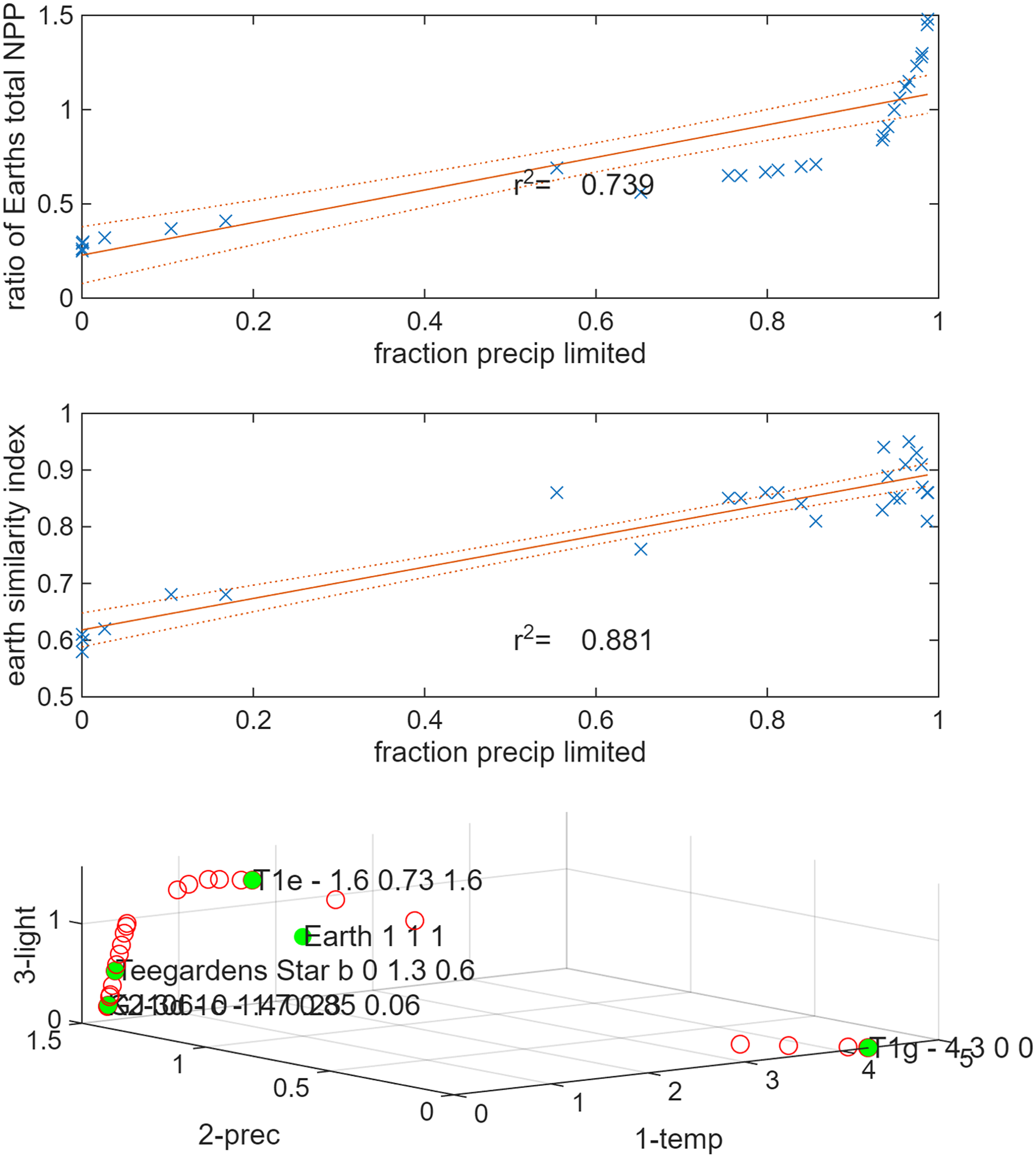
Figure 8. Long description
Panel A: A scatter plot shows the ratio of Earth’s total net primary production (NPP) against the fraction of precipitation-limited areas. The x-axis represents the fraction of precipitation-limited areas, ranging from 0 to 1. The y-axis represents the ratio of Earth’s total NPP, ranging from 0 to 1.5. Data points are marked with blue crosses, and a linear regression line with a coefficient of determination (r-squared) of 0.739 is shown. Panel B: Another scatter plot displays the Earth similarity index against the fraction of precipitation-limited areas. The x-axis represents the fraction of precipitation-limited areas, ranging from 0 to 1. The y-axis represents the Earth similarity index, ranging from 0.5 to 1. Data points are marked with blue crosses, and a linear regression line with an r-squared value of 0.881 is shown. Panel C: A 3D scatter plot illustrates the ratio of planetary surface areas that are temperature-limited, precipitation-limited, and light-limited. The x-axis represents the temperature-limited ratio, the y-axis represents the precipitation-limited ratio, and the z-axis represents the light-limited ratio. Five example planets are highlighted with their respective ratios, such as T1e with ratios of 1.6, 0.73, and 1.6 for temperature, precipitation, and light limitations, respectively.
Discussion
If the biological evolutionary state is a function of cumulative carbon fixed and life began on each of the 29 exoplanets like it had on Earth, life on most of those 29 exoplanets would most likely be evolutionarily behind Earth (with two exceptions discussed below). The majority of our simulations led to most planets at the predicted microbial life stage with the exception of simulations using climates with 1 bar CO2. These very warm, wet planets accelerated NPP production which led about a third of the planets potentially ahead of Earth. However, recent JWST observations showed no evidence of a thick carbon dioxide atmosphere on TRAPPIST-1c (Zieba et al., Reference Zieba, Kreidberg, Ducrot, Gillon, Morley, Schaefer, Tamburo, Koll, Lyu, Acuña, Agol, Iyer, Hu, Lincowski, Meadows, Selsis, Bolmont, Mandell and Suissa2023) or TRAPPIST-1e (Glidden et al., Reference Glidden, Ranjan, Seager, Espinoza, MacDonald, Allen, Cañas, Grant, Gressier, Stevenson, Batalha, Lewis, Long, Wakeford, Alderson, Challener, Colón, Huang, Lin and van der Marel2025), therefore 1 bar CO2 may be unlikely on potentially habitable exoplanets. This raises the question of whether life can exist on an exoplanet with 1 bar CO2 in the atmosphere. CO2 concentrations in the early Earth may have been as high as 10 bar and up to ∼4,000 ppm CO2 in the atmosphere in the Cambrian (Royer, Reference Royer2006), but 1 bar CO2 might not be conducive to land-based life.
Atmospheric composition and uncertainty
Our largest source of uncertainty is the planet’s atmospheric composition, or indeed even whether an atmosphere exists on these planets at all. Planetary mass, volcanic activity, stellar wind and the presence of a magnetic field can all impact the presence and composition of a planet’s atmosphere (Langmuir and Broecker, Reference Langmuir and Broecker2012). Biological processes can also modify the atmospheric composition, as was the case on Earth when photosynthesizing cyanobacteria transformed the atmosphere. Another source of uncertainty is the lack of knowledge of the total near-surface carbon budget of exoplanets. However, we have entered the age of exoplanet atmospheric characterization, and ongoing work may make this possible even for rocky planets like T1e. Recent observations by JWST suggest that TRAPPIST-1b may be an airless world (Greene et al., Reference Greene, Bell, Ducrot, Dyrek, Lagage and Fortney2023; Ih et al., Reference Ih, Kempton, Whittaker and Lessard2023), while TRAPPIST-1c may have a tenuous atmosphere (Lincowski et al., Reference Lincowski, Meadows, Zieba, Kreidberg, Morley, Gillon, Selsis, Agol, Bolmont, Ducrot, Hu, Koll, Lyu, Mandell, Suissa and Tamburo2023; Zieba et al., Reference Zieba, Kreidberg, Ducrot, Gillon, Morley, Schaefer, Tamburo, Koll, Lyu, Acuña, Agol, Iyer, Hu, Lincowski, Meadows, Selsis, Bolmont, Mandell and Suissa2023). These results have been used to constrain estimates and Gialluca et al., Reference Gialluca, Barnes, Meadows, Garcia, Birky and Agol2024 predicted that the outer planets of the TRAPPIST-1 system like T1e have retained >1.5 Earth oceans worth of water (Gialluca et al., Reference Gialluca, Barnes, Meadows, Garcia, Birky and Agol2024). The model assumes an initial loss of water which stopped after ∼380 Myr for T1e as the inner edge of the HZ reached it. They predicted that T1e will have liquid surface water if it initially had more than 2 terrestrial oceans (TO) worth of water (best estimate is it started with 90 TO) (Gialluca et al., Reference Gialluca, Barnes, Meadows, Garcia, Birky and Agol2024). Furthermore, they estimate that the water loss process will create oxygen and that T1e will retain 50% of this oxygen in the atmosphere. It was estimated that the loss of an ocean’s worth of water will generate ∼250 bars of O2, and 1290 bars are estimated on T1e (Earth’s has ∼1 bar atmospheric pressure at sea level. Therefore, T1e likely has abundant liquid water and oxygen, but high atmospheric pressures may constrain life, which we did not consider in our model (but also see (Van Looveren et al., Reference Van Looveren, Güdel, Boro Saikia and Kislyakova2024). However, this area is still highly uncertain and although we assume all 29 exoplanets have atmospheres like that modelled in Sergeev et al. (Reference Sergeev, Fauchez, Turbet, Boutle, Tsigaridis, Way, Wolf, Domagal-Goldman, Forget, Haqq-Misra, Kopparapu, Lambert, Manners and Mayne2022), many models suggest planets like T-1d near the inner edge of the habitable zone are hotter and may have experienced a runaway greenhouse effect (Turbet et al., Reference Turbet, Bolmont, Ehrenreich, Gratier, Leconte, Selsis, Hara and Lovis2020).
Recent findings from the JWST on the spectra of TRAPPIST-1e rule out a thick, hazy atmosphere made primarily of H2 (Espinoza et al., Reference Espinoza, Allen, Glidden, Lewis, Seager, Cañas, Grant, Gressier, Courreges, Stevenson, Sukrit, Knicole, Morris, MacDonald, Long, Wakeford, Valenti, Alderson, Batalha, Challener, Huang, Lin, Louie, Mullens, Valentine, Mountain, Pueyo, Perrin, Bellini, Kammerer, Libralato, Rebollido, Rickman, Sohn and van der Marel2025). Data modeling on secondary atmospheres weakly disfavors a thick atmosphere such as that on Venus, or an airless world like Mars (Glidden et al., Reference Glidden, Ranjan, Seager, Espinoza, MacDonald, Allen, Cañas, Grant, Gressier, Stevenson, Batalha, Lewis, Long, Wakeford, Alderson, Challener, Colón, Huang, Lin and van der Marel2025). These models weakly favor a CH4 rich atmosphere, with a quiet background gas such as N2. However these atmospheric compositions are poor greenhouse gases, meaning that a heavier amount (>1 bar) would be necessary to create enough heating to sustain liquid water on T1e. Atmospheric models of TRAPPIST-1e (Mak et al., Reference Mak, Sergeev, Mayne, Banks, Eager-Nash, Manners, Arney, Hébrard and Kohary2024) and these recent JWST spectra agree that without a greater amount of CO2, the Earth-similar “habitable” temperature of 273.15 K is unlikely which would result in a cold environment. Such findings help constrain our own results as well, as the scenarios where most exoplanets had a higher NPP than earth, and therefore more “advanced” life, required a dense and hazy atmosphere, which may be unlikely for exoplanets orbiting a red dwarf. Only JWST and future space telescopes will resolve this.
Atmospheric composition is related to planetary NPP through the Organic Carbon Burial Rate (OCBR). For example, on Earth, carbon burial has been estimated to be 5–15% of the NPP (Crockford et al., Reference Crockford, Bar On, Ward, Milo and Halevy2023; Derry, Reference Derry2024; Lenton et al., Reference Lenton, Matear, Keller, Scott and Vaughan2018). OCBR is directly tied to the atmospheric oxygen concentration and the resulting oxidation of the atmosphere has been a critical element in impacting the stages of life evolution over Earth’s 4-billion-year evolutionary history. Our simple NPP model and thus our “cumulative NPP” calculation does not incorporate the OCBR nor other long-term geological processes like continental growth, the corresponding supply flux of nutrients (e.g. phosphorus) and sedimentation rate. Thus, our main hypothesis that there is a linear relationship between cumulative carbon fixed and the evolutionary stage of the planet (based partially on Gillman and Wright, Reference Gillman and Wright2014) does not directly link with OCBR/atmospheric composition changes. Future versions of our model should link to OCBR/atmospheric composition changes which would improve the accuracy of our results.
Photosynthetic efficiency
Modifying the model coefficients in the sensitivity study (Table 1) did not change our predicted evolutionary stage away from microbial for T1e. This therefore suggests that the next largest source of uncertainty is which wavelengths of light photosynthesis on each exoplanet would use (<700 nm or <1100 nm). Allowing photosynthesis to use <1100 nm of light (versus <700 nm) greatly accelerated carbon fixed but did not tend to change our estimate of evolutionary stage since most planets were far behind Earth. The most productive pixels in our simulations match empirical results from Ritchie et al. (Reference Ritchie, Larkum and Ribas2018) with anoxic mats producing 658 g DM m-2 yr-1 (vs 740 g DM m-2 yr-1) in our model and oxygenic mats producing 1584 g DM m-2 yr-1 (vs 1795 g DM m-2 yr-1 in our model). Wolstencroft and Raven (Reference Wolstencroft and Raven2002) have suggested more exotic photosystems are needed to take advantage of wavelengths of light >700 nm such as photosystems that use three or four photons, in contrast to two used on Earth. Such systems are complex, and it is not certain that they could evolve, but Ritchie et al. (Reference Ritchie, Larkum and Ribas2018) suggests such systems may not be necessary to survive on planets surrounding red dwarf stars. However, we show (as others have) that ocean covered planets orbiting red dwarf stars would have a competitive disadvantage because NIR energy does not penetrate well into water (Kiang et al., Reference Kiang, Segura, Tinetti, Blankenship, Cohen, Siefert, Crisp and Meadows2007a; Ritchie et al., Reference Ritchie, Larkum and Ribas2018) and most 100% ocean planets would likely be evolutionarily behind Earth for this reason.
Biological evolution on exoplanets hosted by low-mass stars
There are other constraints on the potential biological evolutionary rate for red dwarf star exoplanets that we did not include in our model. Many other factors likely influence evolutionary speed besides productivity and its covariates (solar energy, water, temperature). For instance, M dwarf flaring is an issue that can also affect habitability and life and heightened stellar activity could enhance atmospheric loss (Ridgway et al., Reference Ridgway, Zamyatina, Mayne, Manners, Lambert, Braam, Drummond, Hébrard, Palmer and Kohary2023). UV radiation, for example, has been proposed as a primary control on evolutionary speed on Earth via its role as both a mutagen and selective agent (Davies et al., Reference Davies, Savolainen, Chase, Moat and Barraclough2004; Rothschild, Reference Rothschild1999). However, while UV radiation likely influences the biological evolutionary rate, it is likely not a precondition for productivity / species richness or productivity / evolutionary speed relationships. The LDG applies equally to both high- and low-UV environments (e.g. forest understories; deep marine environments) (Gillman and Wright, Reference Gillman and Wright2014; Hillebrand, Reference Hillebrand2004) and other environmental variables (like high temperatures) also contribute to mutagenesis on Earth (Rohde, Reference Rohde1992). So, while many exoplanets in our solar neighborhood receive only negligible quantities of UV radiation, this probably does not significantly challenge the hypothesized connection between evolutionary speed and productivity. Planets near red dwarf stars might never evolve oxygenic photosynthesis because it confers little competitive advantage (Ritchie et al., Reference Ritchie, Larkum and Ribas2018). We also may be overestimating carbon fixed on tidally locked planets because we assume they fix carbon as long as light is available (unlike Earth plants that pause photosynthesis at night). It is unclear whether plants need a “sleep cycle” and if they do, we would greatly overestimate carbon fixed. Our analysis has used a very simple NPP model and there are more complex models predicting NPP, but we justify this as more complex models all rely on more inputs such as fertility, soil depth, knowledge of plant life parameters, all of which are unknown.
Comparison with Earth and comparison of temperate/arid vs. tropical/boreal ecosystems
Earth, as well as most exoplanets, are majority precipitation limited in terrestrial regions under both Hab1 (100%) and Hab 2 (65%) scenarios. The planets most likely to pass Earth in terms of NPP and most similar to Earth (ESI) are also most likely to be precipitation limited in terrestrial regions (Figure 8). For example, K2-3D with a Hab 2 climate had no temperature limited pixels, 1.4 times as many precipitation limited pixels as Earth and 0.23 times as many light limited pixels. Precipitation limited regions on Earth include most desert, dryland, and temperate systems and often exclude tropical (light limited due to extensive cloud cover) and boreal/arctic systems (temperature limited). We might then hypothesize exoplanets most likely to be ahead of Earth’s NPP would have more temperate/arid ecosystems compared to tropical or boreal systems. Tropical ecosystems have higher NPP than temperate/arid ecosystems and a fully tropical planet would have a higher NPP than a fully temperate/arid planet. However, instead, here we are saying that planets most likely to surpass Earth have more precipitation limited ecosystems (like temperate/arid regions) and their productivity surpasses Earth for reasons other than per pixel productivity such as being older or larger. On Earth, tropical systems are highly biodiverse and there is debate as to their role on biological evolution rates, which is not accounted for in this study. The exoplanets clustered mainly as temperature limited planets (like T1g) and precipitation limited planets (like K2-3D). It is logical to assume that exoplanets hosted by red dwarf (low-mass) stars, with their low energy levels, would be exclusively light limited. However, the Hab1 climates are very dry and the planets will only be light limited if there is sufficient warmth and water.
We assume biological evolution is a function of cumulative carbon fixed, but on tidally locked planets, without diurnal and seasonal cycles, there may be less “temporal” niche space to fill, which could reduce the evolutionary rate. Fewer diurnal or seasonal variations may reduce or increase the evolutionary rate on these planets. Earth’s climate zones are horizontal (i.e. tropical forests between latitudes 20 N and S) while tidally locked planets are vertical (Figure 4c) which could also influence how life may evolve on these planets. Additionally, while our model finds that the majority of exoplanets are less advanced than Earth in terms of biological evolution as a function of cumulative NPP, our model cannot account for climate feedbacks which may yield a greater degree of biological evolution than that demonstrated by our method.
Exoplanets with greatest net primary production and evolutionary stage
We discuss the planets with the greatest cumulative NPP which are summarized in Table 3. The top ranked planets as a function of ratio of cumulative NPP relative to Earth and Earth similarity index (ESI) from the Habitable Worlds Catalog are summarized in Table 4.
Exoplanets with the greatest cumulative NPP reported as a ratio of the exoplanet’s to Earth’s cumulative NPP and the Earth similarity index from the habitable planets catalog. The rankings for NPP ratio and ESI refer to the rankings in the sample of exoplanets reported in Table 3. We then average all three rankings in the final column

Table 4. Long description
A table comparing exoplanets based on distance, NPP ratio, and Earth similarity index. The table has 10 rows and 8 columns. The columns are labeled as follows: Planet, Distance (ly), Distance ranking, NPP ratio, NPP ratio ranking, ESI, ESI ranking, and Overall average. The row labels are the names of the exoplanets. The values in the columns represent the distance in light-years, the ranking of the distance, the NPP ratio, the ranking of the NPP ratio, the Earth similarity index, the ranking of the Earth similarity index, and the overall average ranking. Row 1: Planet, K2-3d; Distance (ly), 143; Distance ranking, 21; NPP ratio, 1.74; NPP ratio ranking, 1; ESI, 0.81; ESI ranking, 19; Overall average, 14. Row 2: Planet, GJ1061c; Distance (ly), 12; Distance ranking, 3; NPP ratio, 1.03; NPP ratio ranking, 2; ESI, 0.86; ESI ranking, 8; Overall average, 4. Row 3: Planet, LP890-9c; Distance (ly), 105; Distance ranking, 19; NPP ratio, 0.85; NPP ratio ranking, 3; ESI, 0.89; ESI ranking, 6; Overall average, 9. Row 4: Planet, Teegardens Star b; Distance (ly), 12.5; Distance ranking, 6; NPP ratio, 0.7; NPP ratio ranking, 4; ESI, 0.95; ESI ranking, 1; Overall average, 4. Row 5: Planet, GJ273b; Distance (ly), 138; Distance ranking, 20; NPP ratio, 0.65; NPP ratio ranking, 5; ESI, 0.81; ESI ranking, 20; Overall average, 15. Row 6: Planet, TOI-715b (N); Distance (ly), 12.3; Distance ranking, 5; NPP ratio, 0.57; NPP ratio ranking, 6; ESI, 0.85; ESI ranking, 13; Overall average, 8. Row 7: Planet, K2-72e; Distance (ly), 216; Distance ranking, 22; NPP ratio, 0.4; NPP ratio ranking, 7; ESI, 0.87; ESI ranking, 7; Overall average, 12. Row 8: Planet, Ross128b; Distance (ly), 11; Distance ranking, 2; NPP ratio, 0.32; NPP ratio ranking, 8; ESI, 0.86; ESI ranking, 9; Overall average, 6. Row 9: Planet, TRAPPIST-1d; Distance (ly), 40.5; Distance ranking, 13; NPP ratio, 0.29; NPP ratio ranking, 9; ESI, 0.91; ESI ranking, 4; Overall average, 9. Row 10: Planet, TRAPPIST-1e; Distance (ly), 40.5; Distance ranking, 15; NPP ratio, 0.21; NPP ratio ranking, 13; ESI, 0.85; ESI ranking, 15; Overall average, 8.
Comparing all of the exoplanets, we hypothesize planet K2-3D has the highest cumulative NPP and evolutionary stage of the 29 planets examined (Figure 7) mainly because of its large size (radius as a ratio of Earths R_E 1.46), old age (6.9 billion years) and warm temperatures (315 K) (Crossfield et al., Reference Crossfield, Petigura, Schlieder, Howard, Fulton, Aller, Ciardi, Lépine, Barclay, Quintana, Christiansen, Schlafly, Kaltenegger, Crepp, Henning, Obermeier, Deacon and Mordasini2015). We may be overestimating the benefits of high temperatures because higher temperatures clearly can negatively affect photosynthesis on Earth (Doughty et al., Reference Doughty, Keany, Wiebe, Rey-Sanchez, Carter, Middleby, Cheesman, Goulden, da Rocha, Miller, Malhi, Fauset, Gloor, Slot, Oliveras Menor, Crous, Goldsmith and Fisher2023) and the temperatures and stellar fluxes may be too high for photosynthesis (Crossfield et al., Reference Crossfield, Petigura, Schlieder, Howard, Fulton, Aller, Ciardi, Lépine, Barclay, Quintana, Christiansen, Schlafly, Kaltenegger, Crepp, Henning, Obermeier, Deacon and Mordasini2015). In Figure S4, we show that adding high temperature thresholds reduces the cumulative NPP of the two leading planets (K2-3D and GJ1061c) leaving no planets surpassing Earth in cumulative NPP at high temperature thresholds of 35 but still surpassing Earth at a more realistic threshold of 40°C and 45°C (based on Earth). In addition, K2-3D’s radius is close to that of mini-Neptune which may have a thick atmosphere, potentially making a surface-dwelling life unlikely (Bonomo et al., Reference Bonomo, Dumusque, Massa, Mortier, Bongiolatti, Malavolta, Sozzetti, Buchhave, Damasso, Haywood, Morbidelli, Latham, Molinari, Pepe, Poretti, Udry, Affer, Boschin, Charbonneau, Cosentino, Cretignier, Ghedina, Lega, López-Morales, Margini, Martínez Fiorenzano, Mayor, Micela, Pedani, Pinamonti, Rice, Sasselov, Tronsgaard and Vanderburg2023). Further, another source of potential error is planetary mass and, therefore, our surface area calculation, are highly uncertain because the radial velocity methods used to estimate mass leads to uncertainty.
We observed from Table 4 that while evolutionary stage and ESI are correlated, ESI is not a direct indicator of cumulative NPP. For example, Teegarden’s star b has the highest ESI of the 29 planets and it is ranked fourth in terms of evolutionary stage. Therefore, while it may be a prime target in terms of similarity to Earth, it is less compelling when considering its potential for biological evolution. #2 GJ1061c is ahead of its sister planets b and d in terms of NPP due to its larger size and higher solar flux. It is also the closest exoplanet to Earth that has a high NPP ratio. #3 LP890-9c sits on the inner edge of the habitable zone making it potentially more similar to Venus than Earth and is a good target for JWST (Gomez Barrientos et al., Reference Gomez Barrientos, Kaltenegger and MacDonald2023). #6 GJ273b is ranked highly in terms of cumulative NPP and ESI, it is also notable that it is the second closest planet to Earth in the list and so it is a promising target for telescopic observations. #7 K2-72e is another promising planet with a high NPP ratio and ESI. One drawback of this planet is that its age is unknown and so its cumulative NPP is not well constrained due to insufficient information regarding its host star.
If we combine distance, ESI and NPP rankings, then Teegarden’s star and GJ1061c are the top ranked multicellular planets (Table 3). Circling back to T1e, we can see it is a good average among the exoplanets, ranking almost in the middle (#15) in terms of distance, NPP and ESI. However, unlike the other planets listed in Table 4, we estimate it would only be at the microbial life stage.
Conclusion
In this paper, we have explored the potential of using the cumulative NPP as a proxy for biological evolution. If life is common in the universe and uses carbon along a similar path as that of Earth, we predict most of our stellar neighborhood to be evolutionary behind Earth, despite the planets often being much older than Earth. Planetary climate (and specifically predicted precipitation) is likely the largest uncertainty in our analysis since the planets are entirely precipitation limited in our most Earth-like scenarios (400 ppm CO2). Anoxic photosynthesis using wavelengths<1100 nm seems likely on T1e since this is possible on Earth (Ritchie et al., Reference Ritchie, Larkum and Ribas2018) and there would be greater evolutionary pressure for this to develop around red dwarf stars peaking in the NIR. Overall, we suggest that observational resources be devoted towards planets GJ 1061c and K2-3d which rank highest under a number of our scenarios because they are bigger, hotter, brighter and older than other planets. However, as shown in this paper, bigger, hotter, brighter and older are not always best for photosynthesis.
We acknowledge that there are several caveats to our analysis (see Section Discussion), several of which may impact the findings of our study. Consequently, there are several avenues of future investigation that we wish to explore. We find that greater temperatures associated with hotter climates are not the best conditions for photosynthesis and so exploring the limitations of temperature and photosynthesis (and alternative photosynthetic pathways) would improve our understanding of this critical habitability parameter.
Another area of future work is to understand how the sample of known exoplanets, which are mostly those that exist in the Solar Neighborhood vary compared to planets across the galactic disk. This would allow us to understand the potential for life on planets outside the Solar Neighborhood; for instance, planets towards the inner Galaxy are likely to be older than those in the Solar Neighborhood and the outskirts due to the “inside-out” formation history of the Milky Way (Iza et al., Reference Iza, Nuza, Scannapieco, Grand, Gómez, Springel, Pakmor, Marinacci and Fragkoudi2024) and so this directly impacts cumulative NPP for planets across the Galaxy as a function of planet age. This also has implications for the concept of the Galactic Habitable Zone, which suggests that there may be regions of the Galaxy that are uninhabitable due to insufficient metallicity which are the building blocks of planets (Gonzalez et al., Reference Gonzalez, Brownlee and Ward2001), or the dangers of nearby supernovae or gamma-ray bursts that deplete atmospheric ozone which otherwise protects land-based life, i.e., terrestrial/vascular plants in this paper (Forgan et al., Reference Forgan, Ilee, Cyganowski, Brogan and Hunter2016; Gowanlock, Reference Gowanlock2016; Gowanlock et al., Reference Gowanlock, Patton and McConnell2011). Understanding how the cumulative NPP interacts with these factors that are related to the galactic environment will help further constrain biological evolution on nearby exoplanets as well as those across larger spatiotemporal scales.
Finally, the most compelling potentially habitable exoplanet targets for spectral characterization in the Solar Neighborhood likely have not yet been discovered. The 29 exoplanets examined in the study are predominantly orbiting low-mass stars due to detection biases. Future telescopes, such as the Habitable Worlds Observatory or the Large Interferometer For Exoplanets, will be able to locate and directly image planets around Sun-like stars. Potentially, these planets might have NPPs more similar to Earth and we could estimate it with these methods.
Supplementary material
The supplementary material for this article can be found at https://doi.org/10.1017/S1473550426100378.
Data availability statement
All data and code to create the figures in this paper can be found at the URL: https://datadryad.org/dataset/doi:10.5061/dryad.37pvmcvvk with a doi:10.5061/dryad.37pvmcvvk.
Acknowledgements
CED was funded through a NASA habitable worlds grant 16-HW16-2-0025 and ZK and CH were funded through NAU/NASA Space Grant program grant #80NSSC20M0041. D.E.S. was supported by a UKRI Future Leaders Fellowship [grant number MR/T040866/1]. We thank Nancy Kiang for advice.
Author contributions
CED and MG came up with idea. ZK, CH, DES and BCW helped research and provided data. All authors contributed to editing.
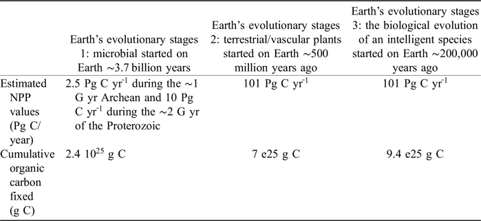

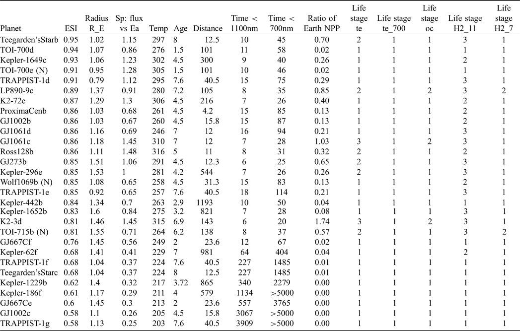


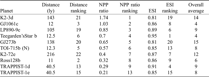


 Open access

