2 Experimental methods

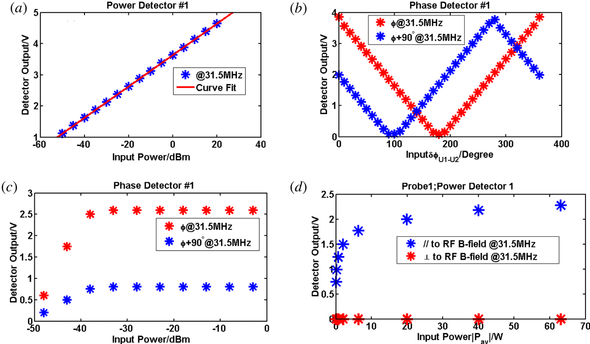
Amplitude and phase are two key properties of an RF wave. The measurement of amplitude and phase can be achieved using a logarithmic RF detector. The RF amplitude is converted into a direct current (DC) signal using the power detector stage from AD8307 (http://www.analog.com/media/en/technical-documentation/data-sheets/AD8307.pdf) as shown in figure 1(a). Power density in the near field of the probe could be calculated using the data obtained from AD8307. It is a complete 500 MHz monolithic demodulating logarithmic amplifier based on the progressive compression (successive detection) technique, providing a dynamic range of 92 dB to $\pm 3$  dB law conformance and 88 dB to a tight $\pm 1$  dB error bound at all frequencies up to 100 MHz.

In the coaxial transmission line, the time-averaged Poynting flux ( $P$ ) at the probe location (the probe located at the inner radius of the outer conductor of the coaxial transmission line) can be calculated by the equations of an Ampere circuit and Gauss’s law. Power density in the near field of a probe can be calculated if the relationship between the amplitude of probe and the Poynting flux ( $P$ ) at the probe location of coaxial transmission line is known.

Figure 1.

Essential parameters of phase and power detectors. (a) The output of the amplitude detection stage versus the input RF power; (b) the output of the phase detection stage as a function of the input phase difference between U1 and U2 and between $\text{U}1+90$ and U2@31.5 MHz; (c) input power is the power put into the phase detector. When the input power is larger than $-37$  dBm, the output of the phase detector stage is stable, as shown; (d) probe orientation determines polarization of the measured RF wave (the probe has been located in the coaxial transmission line).

For a standard function, we can use $y=\sin (kx-\unicode[STIX]{x1D714}t+\unicode[STIX]{x1D6F7}_{0})$ to describe it, defining $\unicode[STIX]{x1D719}=kx-\unicode[STIX]{x1D714}t+\unicode[STIX]{x1D6F7}_{0}$ , where $x$ is the probe location, $\unicode[STIX]{x1D714}$ is the angular frequency of RF wave, the derivative of $x$ on both sides gives $\text{d}\emptyset /\text{d}x=k$ ; this equation has a frequency-independent quantity. The phase difference between the probes $\text{d}\emptyset$ can be obtained from the AD8302 documentation (http://www.analog.com/media/en/technical-documentation/data-sheets/ad8302.pdf), where $\text{d}x$ is the probe distance. Phase detector had been used to detect the phase difference of two RF signals, it can convert the information of the phase difference to DC signals. Because of the nature of AD8302, it can only detect the phase difference from $0^{\circ }$ to $180^{\circ }$ . For practical purposes, we need to measure the phase difference up to $360^{\circ }$ . This is the same technique as has been used in for the B-dot measurements in the ASDEX Upgrade (Ochoukov et al. Reference Ochoukov2015). As shown in figure 1(b), $90^{\circ }$ of phase difference is used for the input signal to achieve this goal. The working position of the phase detector is influenced by the strength of the input power. Only when the input power is higher than $-37$  dBm is the output of the detector believable (figure 1 c).

There is a close relationship between the polarization of the electromagnetic wave and the direction of the B-dot probes. When the magnetic probe coil is placed perpendicular to the direction of the magnetic field, the strength of the magnetic probe coupling voltage signal exponentially increases as the incident power increases. When the magnetic probe coil is placed parallel to the magnetic field, the signal strength of the magnetic probe is close to 0 (figure 1 d). The ion cyclotron frequencies in EAST are 31.5 MHz (B antenna) and 34 MHz (I antenna), respectively. In order to avoid the influence of high-frequency electromagnetic waves (low hybrid waves, ion cyclotron waves), a band pass filter has been used to limit the working frequency of the diagnostic system to 3–50 MHz. A tokamak’s internal signal transmission uses a high-temperature, high-vacuum, $50\unicode[STIX]{x1D6FA}$ coaxial transmission line (https://accuglassproducts.com/product.php?productid=16346&cat=0&page=1) to accommodate the EAST internal environment. Vacuum coaxial feedthrough (https://www.accuglassproducts.com/files/PDF/Catpages/34.pdf) is used to transmit RF signals from the tokamak to the atmosphere for data acquisition and analysis.

3 Specific location and detailed structure of the probe

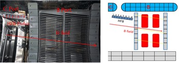
In order to further understand the characteristics of the ion cyclotron waves inside EAST, we installed eight magnetic probes as shown in figure (figure 2). The location of the probes is 31 cm above the midplane, radially 6 cm behind the ion cyclotron antenna limiter and toroidally in the middle of the B and C ports. The angle between the direction of the magnetic probe array and the toroidal direction is $6^{\circ }$ , mainly to ensure the same direction as the Faraday screen of the antenna, shown by the yellow line in the figure. In order to measure ICRF waves with different polarization directions, we place the magnetic probes perpendicular and parallel to the background magnetic field respectively. B-dot probes placed parallel to the background magnetic field are used to measure fast waves, and B-dot probes placed perpendicular to the background magnetic field are used to measure the slow waves. The direction of the background magnetic field is shown by the red arrow. When the central magnetic field strength is 2 T and the plasma current is 500 kA, the direction of the background magnetic field coincides with the direction of the antenna Faraday shield. The operating frequency of the ion cyclotron antenna B is 31.5 MHz and consists of four current straps which are distributed in a $2\times 2$ manner, so we consider them to be the left and right straps when considering the influence of the phase difference between the current straps on the spectrum.

Figure 2.

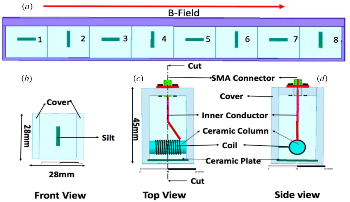
The figure above shows the distribution of magnetic probes in EAST. The magnetic probes are distributed on the right side of the B antenna. The direction of the background magnetic field is shown by the red arrow ( $B>0$ ). There are four pairs of magnetic probes, which are parallel and perpendicular to the background magnetic field respectively. The probes parallel to the background magnetic field are labelled ‘1’ ‘3’ ‘5’ ‘7’, and are called ‘fast wave’ probes. The probes perpendicular to the background magnetic field are labelled ‘2’ ‘4’ ‘6’ ‘8’, and are called ‘slow wave’ probes. The magnetic probes are located 6 cm behind the antenna limiter. The yellow line represents the Faraday screen.

The B-dot probe has been build based on the ASDEX Upgrade probe design (Ochoukov et al. Reference Ochoukov2015), and the specific structure of it is shown in figure 3. The entire outer structure of the B-dot probe is a stainless steel housing. The length and the width of the stainless steel housing are 28 mm and the height is 45 mm. At the bottom of the housing there is a 2 mm wide and 12 mm long silt where the electromagnetic wave can enter steel cavity. There is a 1 mm thick ceramic plate inside the silt to protect the spiral coil in the stainless steel cavity. The coil is made of 0.5 mm diameter copper wire, the diameter of the coil is 8 mm and it is wound on a ceramic rod with a diameter of 8 mm. One end of the coil is connected to the stainless steel housing and the other end is linked by a $50\unicode[STIX]{x1D6FA}$ sub-miniature-A (SMA) connector. All probes were mounted on stainless steel probe holders to facilitate mounting of these probes on EAST (figure 3 a).

Figure 3.

(a) The distribution of four pairs of magnetic probes, parallel and perpendicular to the background magnetic field respectively; (b) a top view of the probe from the plasma side, the silt of the probe can been seen; (c) a front view of the probe with internal components shown; (d) a side view of the probe, one side of the coil is connected to the stainless steel cover.

4 Test experimental platform and simulation

4.1 Experimental platform

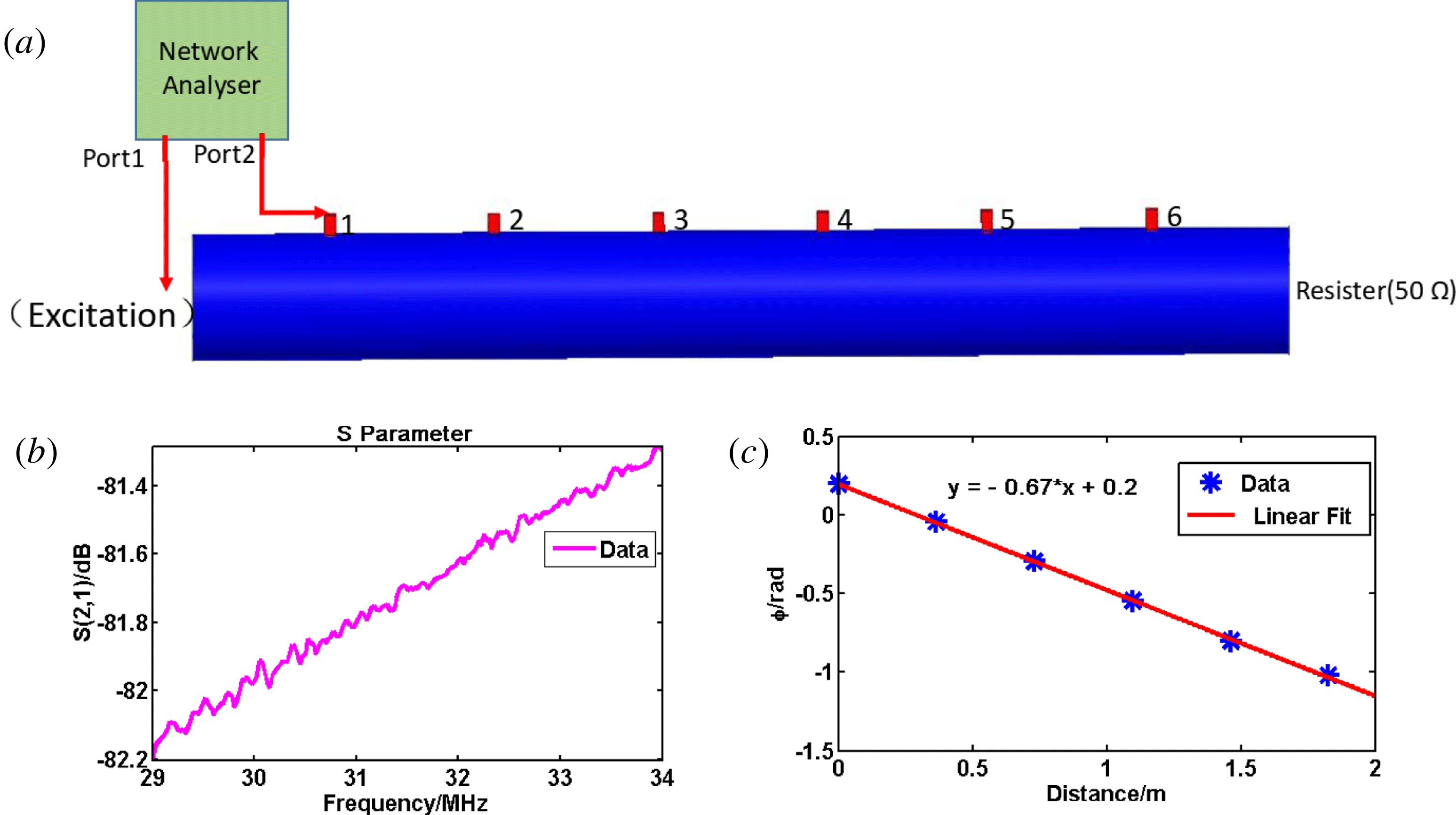
Test experiments were performed before the spring of 2017 campaign. The purpose of the test experiments was to determine the attenuation coefficient of the probe and prove that the diagnostic system does have the ability to acquire the spectrum of a RF wave. There are two methods to achieve this goal. In the first method, the network analyser was used. The scheme of the diagnostic system in the laboratory is shown in figure 4(a). Port 1 of the network analyser is used to give the coaxial transmission line an excitation and port 2 is connected to the probe. The phase difference between port 1 and port 2 of the network analyser is then obtained. When port 2 of the network analyser is changed to a different probe and the phase different of adjacent probes is obtained. The distance between the probes was also measured. Another side of the coaxial transmission line is connected to a resistor of $50\unicode[STIX]{x1D6FA}$ . The $S$ parameter and wavenumber $k$ of the RF waves (source frequency $=$ 31.5 MHz) are plotted in figures 4(b) and 4(c) respectively.

The value of $S$ (2, 1) is approximately $-81.7$  dB at 31.5 MHz, and it increases with increasing frequency of the RF source in the test experiment. In the experimental platform, the excitation in the coaxial transmission line is 10 mW. This means that the power coupled by probe is very small. The noise in the laboratory is high enough to cause distortions in the measurements of the $S$ parameter. Nevertheless, the value of $|k|=0.67$ measured in the test experiments is almost in agreement with the expected value for a wave propagating in the coaxial transmission line ( $k=2\unicode[STIX]{x03C0}f/c=0.66~\text{m}^{-1},f=31.5\times 10^{6}~\text{Hz}$ ).

Figure 4.

Network analyser was used to get the attenuation coefficient and the phase difference between adjacent probes. (a) Simplified test experiments in the laboratory; (b) $S(2,1)$ is the value of the attenuation coefficient of probe ‘1’ positioned at the radius of the outer conductor of the $50\unicode[STIX]{x1D6FA}$ coaxial line, the pink curve corresponding to measurement results is shown for the orientation of the probe parallel to the excited RF $B$ -field; (c) the parallel wave number $|k|$ of a RF wave was 0.67, the blue dots are measurements and the solid red line is a linear fit and the frequency is 31.5 MHz.

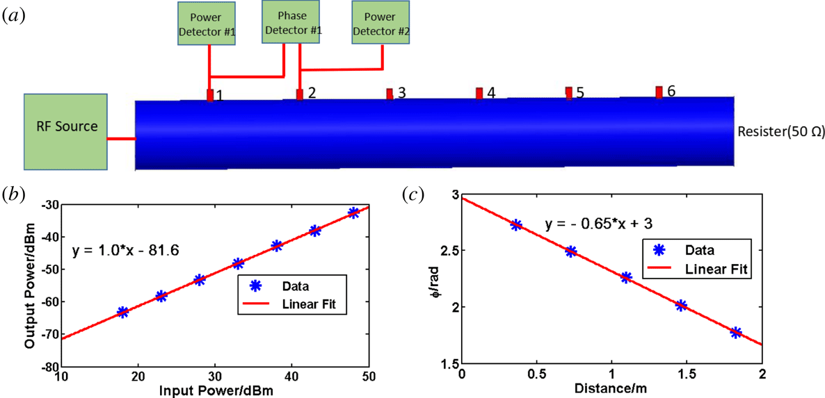
In the second method, a radio frequency source and power/phase detector are used instead of the network analyser in the experimental laboratory. The phase detector (AD8302) was used to get the phase difference between the probes. The power detector (AD8307) was used to obtain the amplitude of the RF waves. The probes were placed at the radial location of the transmission line outer conductor. The scheme of the diagnostic system is shown in figure 5(a).

The attenuation coefficient of the probe and parallel wavenumber $k$ of the RF waves (source frequency $f=31.5$  MHz) have been obtained by AD8307 and AD8302 separately (figures 5 b and 5 c). It is clear that $-81.6$  dB is the value of the attenuation coefficient of the probe when the frequency of the RF source is 31.5 MHz. The result obtained by the power detector is almost the same as that by the network analyser. The value $|k|=0.65$ was calculated in the test experiments using the results of the phase detector. It agrees well with the expected value of the wavenumber $k=0.66$ .

Figure 5.

The frequency of the RF source is 31.5 MHz. (a) The model of the simplified experimental platform in the laboratory, the power detector/phase detector was used to get the attenuation coefficient and the phase difference; (b) the value of the attenuation coefficient of probe ‘1’ positioned at the inner radius of the outer conductor is $-81.6$  dBm, and the orientation of the probe parallel to the excited RF $B$ -field; (c) the parallel wavenumber $|k|$ of the RF wave is 0.65, the blue dots are measurements and the solid red line is a linear fit.

4.2 Simulation

To ensure the reliability of the platform’s experimental results, a high-frequency structure simulator (HFSS) as a simulation software has been used. The material quality of the electrical components in the HFSS simulation model is the same as in reality. In the simulation model, the coaxial transmission line with an outer radius 115 mm and inner radius 50 mm is placed in air, and the impedance of the coaxial transmission line is $50\unicode[STIX]{x1D6FA}$ . One side of the transmission line is used to excite waves at the chosen frequency. Another side of the coaxial transmission line is terminated with a $50\unicode[STIX]{x1D6FA}$ resistor which can be set to produce no reflection. The B-dot probes in the simulation have the same structure as the probe used in the EAST experiments, the specific structure and materials of the probe were described in sector 2. These probes were placed at the inner radial location of the transmission line outer conductor and oriented parallel (//) to the excited $B$ -field orientation. The distance between the probes is 300 mm. At the end of the SMA connector of the probe is the wave port which was used to couple power from the coils of the probe.

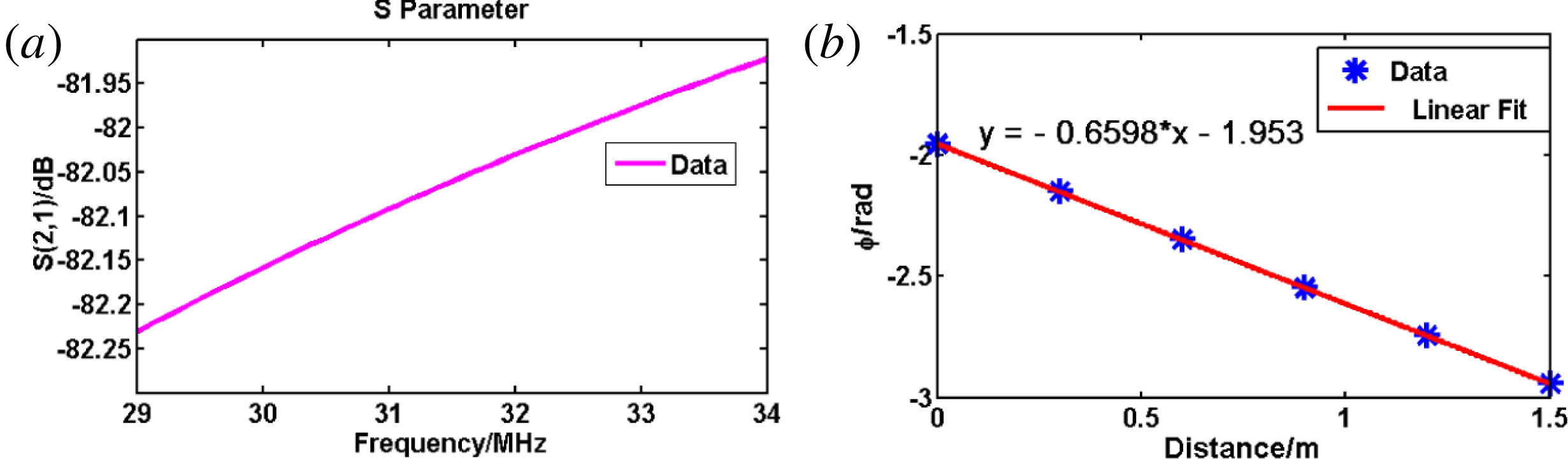
Using the simulation code, one can get the attenuation coefficient of the probe and the phase difference between the adjacent probes. All the probes have nearly the same attenuation coefficient in the simulation. $S_{21}$ is exhibited in figure 6(a). In the simulation the value of $S_{21}$ is approximately $-82$  dB when the frequency is 31.5 MHz, and it increases with increasing frequency of the RF source. The distance between the adjacent probes is 300 mm. The phase difference between the adjacent probes can also be calculated. The parallel wavenumbers can be obtained using the equation $k=\text{d}\emptyset /\text{d}x$ . The RF wave (source frequency $f=31.5~\text{MHz}$ ) propagates in the coaxial transmission line in air (it is assumed that the refractive index of the air is 1). Figure 6(b) is plotted using the simulation results. The simulated $k_{//}=0.6598~\text{m}^{-1}$ agrees well with the expected value $k=\unicode[STIX]{x1D714}/c=2\unicode[STIX]{x03C0}\times (31.5\times 10^{6}~\text{Hz})/(3\times 10^{8}~\text{m}~\text{s}^{-1})=0.66~\text{m}^{-1}$ , where $c$ is the speed of light in a vacuum, $\unicode[STIX]{x1D714}$ is the angular frequency of the ICRF.

Figure 6.

(a) $S(2,1)$ is the value of the attenuation coefficient of probe ‘1’ positioned at the inner radius of the outer conductor of the $50\unicode[STIX]{x1D6FA}$ coaxial line, and the pink curves corresponding to simulation results are shown for the orientation of the probe parallel to the excited RF $B$ -field; (b) the parallel wavenumber $|k|$ of the RF wave was 0.6598, the blue dots are simulation results and the solid red line is a linear fit. The frequency is 31.5 MHz.

In the test platform, we used the network analyser and power/phase detector to detect the ion cyclotron wave characteristics (the probe attenuation coefficient, wavenumber $k$ and wave polarization), and the results obtained by these two methods are very similar. In order to assure the reliability of the results in the test experimental platform, we used HFSS software to establish a three-dimensional simulation model. In the three-dimensional model of HFSS, its structure and material were chosen to be exactly the same as in the experimental platform. The results obtained by the simulation model are consistent with the results from the experimental platform, and this confirms the reliability of the B-dot probe based diagnostic system. Finally, the diagnostic system was installed on EAST to test the characteristic of ion cyclotron waves.

5 Experiment results and discussion

First experimental data with new HFB probe array diagnostic were obtained during the 2017 spring experimental campaign on EAST. The plasma parameters are on-axis magnetic field, $B_{t}=-2T$ , total plasma current $Ip=400~\text{KA}{-}600$  KA. The negative direction of the magnetic field means it is in the opposite direction to the plasma current direction. The hydrogen fraction (H/D) is approximately 5 %.

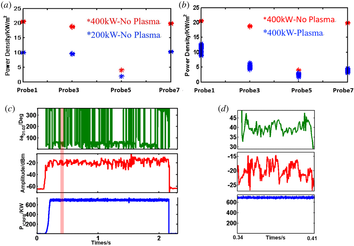
First and foremost, it is important to know what kind of response the probes have as a function of the applied ICRF power and to verify whether this remains linear as the power goes up. A typical vacuum response of four of the HFB probes is shown in figure 7(a). The ICRF power was 200 kW and 400 kW respectively. The amplitude response of the individual probes, when expressed in units of power, is linearly proportional to the applied ICRF power, as the power coupled by the probe is twice as high when the ICRF power increases from 200 kW to 400 kW. Shown in figure 7(b) are two shots with the same ICRF power but one shot is with a plasma and another is in a vacuum. The power density of waves in a vacuum is much higher than it is in a plasma. The likely reason is that a large part of the ICRF power was absorbed by the plasma. We also found that the power density measurements appear to be ‘noisy’ in plasma compared to their vacuum values. This indicates the interaction between the plasma and the ICRF waves.

Figure 7.

The toroidal distribution of key parameters measured by the HFB diagnostic. (a) The power density distribution in a vacuum is displayed at two levels of power; (b) the power density distribution in a vacuum and a plasma with the same power; (c) a typical response of the HFB probe signals in an L-mode plasma, the measured HFB response of the phase between probes 1 and 3 is shown at the top of the picture, the measured HFB probe ‘7’ amplitude response is shown in the middle of the picture and the applied ICRF power is shown in the bottom of the picture; (d) it is the expansion of 0.34 s–0.41 s of (c).

The purpose of the HFB diagnostic is to help study ICRF wave fields in the presence of a plasma, and a typical signal response during an L-mode discharge is shown in figure 7(c,d). The ion cyclotron wave power is slightly disturbed under the influence of the plasma, but this tiny perturbation should not cause such a large disturbance of the B-dot probe signal. The interaction between plasma and ICRF waves is a leading element for the fluctuation of the ion cyclotron wave signals. The phase difference between the probes can be used to estimate the wavenumber $k$ . Although there is a phase jump from $0^{\circ }$ to $360^{\circ }$ , the phase difference value is mainly concentrated around $40^{\circ }$ which results in $k_{//}=12.5~\text{m}^{-1}$ . The domain value of the wavenumbers of antenna B is $k_{//}=13~\text{m}^{-1}$ , which is very similar to the experimental results.

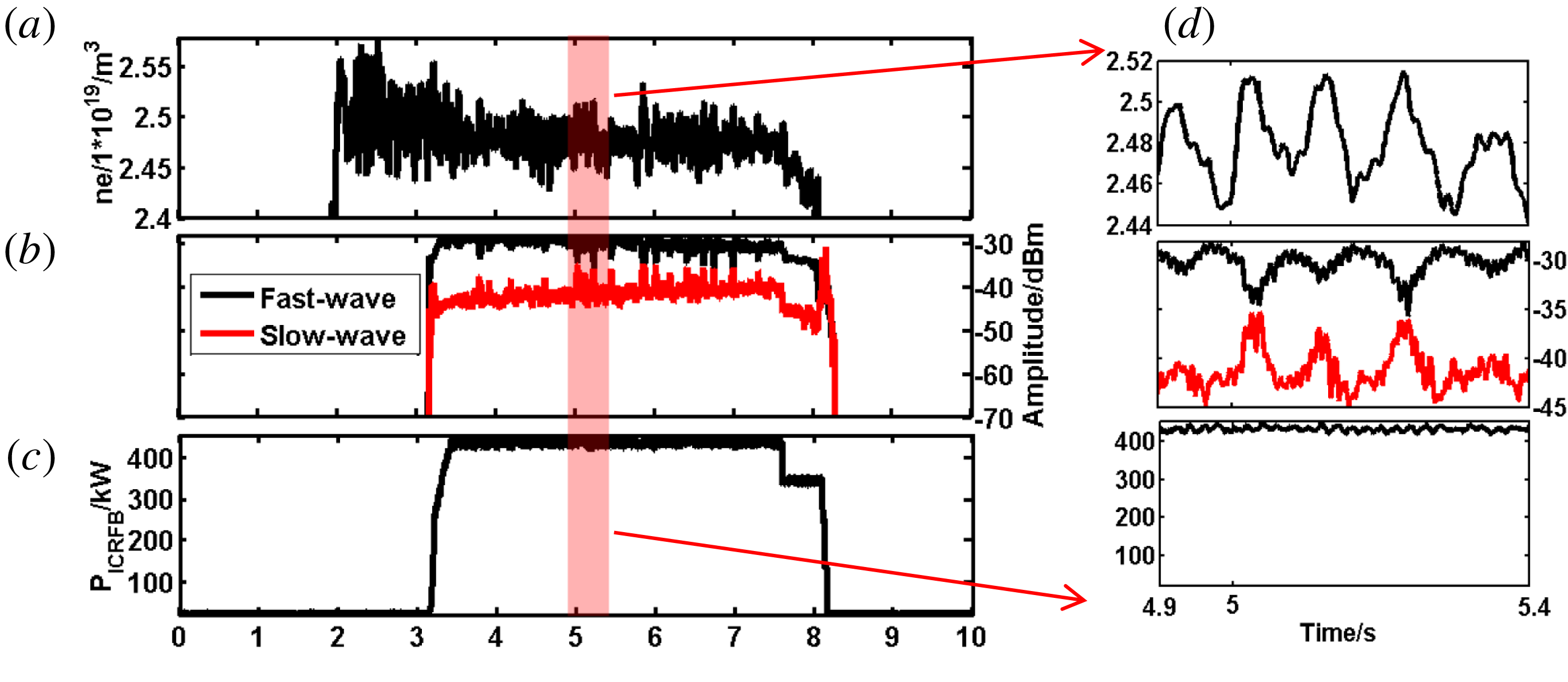
Because of the disadvantages of the slow wave, it is preferable to have its amplitude low during heating of the plasma. The measurements show that the amplitude of a fast wave is approximately ten time higher than that of a slow wave close to the antenna (figure 8 b). The fast wave was characterized by the probe labelled ‘7’ and the slow wave was characterized by the probe labelled ‘8’ which are shown in figure 2(b). From figure 8(d) we can conclude that the fluctuation of the core electron density has a certain relationship with the amplitude of the ICRF waves in the near field of the antenna. The amplitude of the fast wave goes down when the core electron density goes up, and the tendency of the slow wave is opposite to the fast wave. For the fast wave, the likely reason is that more power is coupled by the plasma when the core electron density increases as the edge electron density is influenced by the core, hence the amplitude of the fast ICRF waves is decreased in the edge area. Plasma density at the edge plays a significant role in the fluctuation of the slow waves as the dispersion relationship of the slow wave is closely related to the electron density. Because one of the transmitters was switched off at approximately 7.6 s, there is a jump in the values (figure 8 c). The same tendency is seen in the power detected by the probes.

Figure 8.

Influence of plasma density on the amplitudes in the near field. (a) The core electron density by Thomson scattering (core); (b) the fast and slow wave amplitudes in the near field of the antenna; (c) the power of ICRF waves in port B; (d) time span of the left picture between 4.9 s and 5.4 s, and the relationship between the amplitude and the core plasma density is clear.

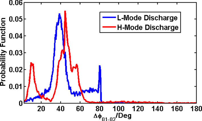
In order to observe the distribution of the parallel wavenumbers $k_{//}$ , we plotted a distribution of the phase difference between probes (figure 9). This distribution map is a probability distribution function of phase difference between the B-dot probes. The ordinate axis represents a normalization value of the number of data points in different groups, and only represents the probability in this phase difference value.

In L-mode discharges, the measured wave fields have a well-defined phase distribution. The main contribution to the phase difference is observed close to $40^{\circ }$ corresponding to the parallel wavenumber $k_{//}=12.5~\text{m}^{-1}$ and the expected value is $k_{//}=13~\text{m}^{-1}$ . In H-mode discharges, a different distribution of the phase difference is observed compared to the L-mode discharges. There are at least two reasons which can account for the domain parallel wavenumbers changing, namely (i) the profile of the antenna current along the conductor (Bures et al. Reference Bures, Jacquinot, Start and Brambilla1990); (ii) the distance between the antenna and plasma (the toroidal variation of the current density can be rewritten in a plasma $\unicode[STIX]{x1D70E}_{\unicode[STIX]{x1D711}}^{\text{plasma}}(\unicode[STIX]{x1D711})=\unicode[STIX]{x1D70E}_{\unicode[STIX]{x1D711}}(\unicode[STIX]{x1D711})\text{e}^{-k_{//}d}$ , with $d$ is the antenna–plasma distance (Savona Reference Savona2017)). The distance between the plasma and antenna and the profile of the antenna current along the conductor vary strongly during edge localized modes (ELMs) in H-mode discharges.

There are two problems appearing in the measurement of the phase difference between two B-dot probes, mainly related to the characteristics of the chip AD8302. First, as mentioned in Section 2, when the input signal strength of the chip AD8302 is less than $-37$  dBm, the phase detector does not work properly (in most of the cases, the input signal of the phase detector is larger than $-30$  dBm). Second, when one of the input signals is significantly larger than the other (signal strength differs by 10 dB), the measurement result is affected. In the next experiment we will use a signal amplifier to solve the first problem. For the second problem, the results with a phase difference with too large a power difference of the probes will be omitted.

Figure 9.

The probability of the phase measurement between probes 05 and 07 in an L-mode discharge and H-Mode discharge.