





1. Introduction
Helical vortices appear in a variety of applications, in particular in the wake of rotors, such as those used for wind energy harvesting, helicopter flight and propulsion of aircraft and marine vehicles. With their conceptual simplicity, they also represent basic flow configurations for the study of fundamental vortex interactions and instabilities, which have been the subject of a large number of studies.
An infinite thin-cored helical vortex conserves its geometry in time, while translating in the direction of its axis and rotating around it through self-induction (Widnall Reference Widnall1972). In the appropriate reference frame it represents a stationary flow in the inviscid limit.
Helical vortices are unstable, and various instability mechanisms have been identified. The interaction between neighbouring helix loops leads to the growth of long-wave perturbations (with respect to the core dimensions), with little change to the core structure, which can be related to the pairing instability of an array of parallel vortices. This was analysed theoretically with a filament approach by Widnall (Reference Widnall1972), Gupta & Loewy (Reference Gupta and Loewy1974) and Okulov & Sørensen (Reference Okulov and Sørensen2007), and experimentally by Quaranta et al. (Reference Quaranta, Bolnot and Leweke2015, Reference Quaranta, Brynjell-Rahkola, Leweke and Henningson2019).
Short-wave instabilities, which involve internal perturbations of the vortex core, were also found for helical vortices. They are caused by interactions of neutral/damped vortex modes (Kelvin modes) through core deformations induced by an external strain (elliptic instability) or the vortex curvature (curvature instability). Their wavelengths along the vortex axis are of the order of the core size. Short-wave instabilities of a helical vortex were studied theoretically by Hattori & Fukumoto (Reference Hattori and Fukumoto2009, Reference Hattori and Fukumoto2012, Reference Hattori and Fukumoto2014) and Blanco-Rodríguez & Le Dizès (Reference Blanco-Rodríguez and Le Dizès2016, Reference Blanco-Rodríguez and Le Dizès2017), and were found in the numerical simulations of Brynjell-Rahkola & Henningson (Reference Brynjell-Rahkola and Henningson2020) and Xu et al. (Reference Xu, Delbende, Hattori and Rossi2025). Clear experimental evidence is still missing; some preliminary visualisations from a rotor wake were shown by Leweke et al. (Reference Leweke, Quaranta, Bolnot, Blanco-Rodríguez and Le Dizès2014).
Theoretical and numerical work on short-wave instability has mostly considered simple vortex models, like the Rankine and Lamb–Oseen/Batchelor vortices, with constant and Gaussian core vorticity and axial flow distributions, respectively, and for the case of helical vortices, the core sizes are often not small compared with the helix radius. Vortex profiles that are more representative of the tip vortices generated by lifting surfaces, such as aircraft wings, may result in significantly different vortex modes and associated short-wave instability, as shown, e.g. for the case of straight vortices by Fabre & Jacquin (Reference Fabre and Jacquin2004a ) and Feys & Maslowe (Reference Feys and Maslowe2014).
The present work is based on a rotor wake experiment, in which the core radius of the helical vortex is only a few per cent of the helix radius, and the vorticity profile is qualitatively different from Gaussian, with a major part of the total circulation located in the region outside of and surrounding the viscous core. The experiment and accompanying numerical simulation and theoretical calculation are described in § 2. Experimental observations of the short-wave instability are provided in § 3, followed by a comparison with results from numerical simulation and stability analysis of the same flow in § 4. Both the experiments and numerics show the existence of a new unstable short-wave displacement mode. In § 5, a theoretical analysis considers relevant Kelvin modes and their interactions for the experimentally measured profiles and discusses possible mechanisms leading to this instability. Conclusions are presented in § 6.
2. Methodology
2.1. Experimental set-up and methods
Experiments were performed in a recirculating free-surface water channel with a test section of 38 cm (width)
 $\times$
50 cm (height)
 $\times$
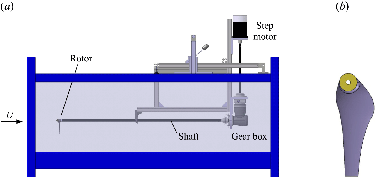
150 cm (length). A helical vortex was generated using a one-bladed rotor, mounted on an ogive-tipped shaft of 1.5 cm diameter, and driven externally by a computer-controlled stepper motor through a gear box (figure 1
 $a$
). The blade geometry (figure 1
 $b$
) is based on the low-Reynolds-number airfoil A18 by Selig et al. (Reference Selig, Guglielmo, Broeren and Giguère1995). It is designed to operate in the wind turbine regime and to produce a constant radial circulation distribution, in order to generate a highly concentrated tip vortex. The rotor has a radius
 $R_0$
= 8 cm and a tip chord
 $c$
= 1 cm. Additional details on the design methodology and experimental protocols are provided in Bolnot (Reference Bolnot2012) and Quaranta et al. (Reference Quaranta, Bolnot and Leweke2015). In the present configuration, the blade rotated at a frequency
 $f$
= 6.25 Hz, and the channel flow had a uniform free-stream velocity
 $U$
= 37.5 cm s−1, yielding a tip-chord-based Reynolds number
 ${Re} = 2 \pi R_0fc/\nu \approx 30\, 000$
, where
 $\nu$
is the kinematic viscosity.
The structure and evolution of the helical vortex were characterised by dye visualisations and velocity measurements. For the visualisations, fluorescent dye was painted on the blade tip prior to rotation, and then illuminated by LED panels emitting at a wavelength of 480 nm. Video sequences were recorded with a standard digital camera operating at 25 images per second. They provided information about the helix geometry (radius
 $R$
, pitch
 $h$
) and the perturbations related to the short-wave instability (structure, wavelength). Radial profiles of swirl and axial velocities of the tip vortex were measured by high-resolution stereoscopic particle image velocimetry (PIV), using a Nd-YAG double-pulsed laser and acquisition system from Dantec Dynamics. Their Dynamic Studio 8 software was used to obtain the three velocity components in the mid-plane of the rotor wake, focusing on a vortex cross-section located approximately half a helix pitch downstream of the rotor plane. Phase-averaged velocities were obtained from 2000 instantaneous PIV fields.
(
 $a$
) Experimental set-up (side view of the water channel test section) and (
 $b$
) the rotor blade geometry.

2.2. Numerical set-up and methods
The flow is simulated using an in-house code based on a spectral/spectral-element approach (Karniadakis & Triantafyllou Reference Karniadakis and Triantafyllou1992; Thompson et al. Reference Thompson, Hourigan and Sheridan1996). In radial planes, the flow is captured using a nodal spectral-element discretisation with refinement in the vicinity of the vortex, while the variation in the direction of the helix axis is represented by a Fourier expansion. The grid spacing is
 $\sim$
0.002
 $R$
in both the radial and axial directions near the vortex to resolve the very compact core. Preliminary testing was undertaken using increased resolution in both the radial and axial directions to ensure that this resolution is sufficient to properly resolve the flow. A single helix loop is simulated and the flow is assumed periodic in the direction of the helix axis, which prevents the development of long-wave pairing instabilities, whose modes are not periodic, but out of phase, over one helix loop. Computation follows temporal evolution rather than spatial development as in the experiments; a correspondence can be established via the helix convection speed
 $hf$
. Simulations are run with 5120 5
 $\times$
5 conforming quadrilateral spectral elements to capture the variation across two-dimensional axial slices extended to three dimensions with 256 planes in the axial direction. This equates to
 $\sim$
21 million mesh points. The grid extends radially to
 $4R$
. Note that the mesh is locally radial in the neighbourhood of the helix with circular arc segments in the azimuthal direction to avoid artificially perturbing the flow development from mesh-associated discretisation errors.
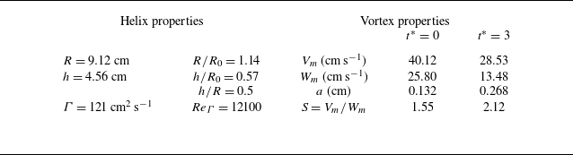
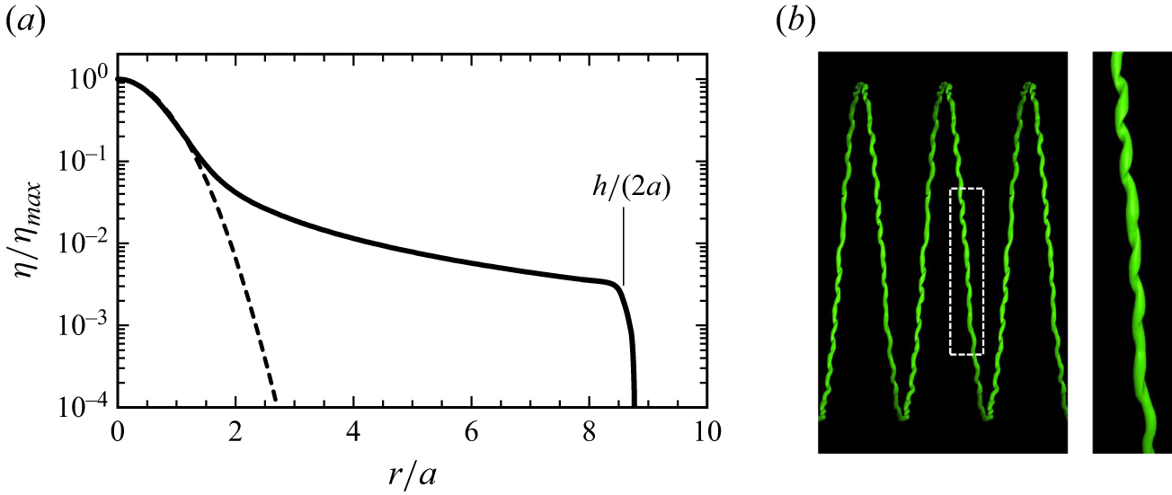
Simulations are initialised using the helix properties and velocity distributions measured in the experiments (table 1). Because the azimuthal velocity component falls off slowly far beyond the vortex core region, the initial condition is constructed from the more compact fitted azimuthal and axial vorticity distributions, truncated at a distance
 $h/2$
from the vortex centre (figure 5
 $a$
), in order to avoid overlap from neighbouring loops. The helix radius
 $R$
and initial maximum swirl velocity
 $V_m$
of the vortex are set to unity in the simulations, which defines the non-dimensional time as
 $t^*=tV_m/R$
, with
 $t^*$
= 0 corresponding to the instant when the tip vortex passes the measurement location.
Properties of the unperturbed helical vortex.

Table 1. Long description
A table comparing helix and vortex properties. The table has two main sections: Helix properties and Vortex properties. The Helix properties section includes the following rows: Radius (R) is 9.12 centimeters, height (h) is 4.56 centimeters, and circulation (Γ) is 121 square centimeters per second. The Vortex properties section is divided into two columns, t* = 0 and t* = 3, each containing the following rows: Vm (velocity) in centimeters per second, Wm (velocity) in centimeters per second, a (radius) in centimeters, ReΓ (Reynolds number), and S (ratio of Vm to Wm). For t* = 0, Vm is 40.12 centimeters per second, Wm is 25.80 centimeters per second, a is 0.132 centimeters, ReΓ is 12100, and S is 1.55. For t* = 3, Vm is 28.53 centimeters per second, Wm is 13.48 centimeters per second, a is 0.268 centimeters, ReΓ is not provided, and S is 2.12.
In the experiments, short-wave perturbations appear obvious at a distance corresponding to
 $t^*=6$
. Therefore, a numerical stability analysis was carried out for the simulated flow frozen at
 $t^*=3$
(after shifting to the frame of reference in which the helix is stationary), by adding a low-amplitude white-noise perturbation to trigger the growth of instabilities, and determining the most unstable modes as function of wavenumber along the vortex axis, using the linearised evolution equations. Determination of the axial modes is achieved by rotating each axial plane so that the helical vortex is lined up between planes – effectively, the helix is unwound into a straight vortex. This allows the axial modes to be determined, which can then be isolated prior to rewinding the helix.
2.3. Theoretical calculation for elliptic instability
Using the experimentally measured helix geometry and velocity profiles, including swirl velocity
 $V(r)$
and axial velocity
 $W(r)$
, as initial input, the unperturbed numerical evolution yields these distributions at any subsequent time. In line with the numerical stability analysis, we take the fields at
 $t^*=3$
as the base flow for theoretical calculations. Variables in the base flow are non-dimensionalised by the core size,
 $a$
(the distance from the core centre to the maximum cross-sectional azimuthal velocity), and the angular velocity in the vortex centre,
 $\varOmega _0$
, at
 $t^*=3$
.
In the theory, perturbations developing within the vortex core are assumed to be composed of waves (also called Kelvin modes), expressed for the velocity and pressure fields
 $(\boldsymbol{u}',p')$
in the form
 \begin{equation} (\boldsymbol{u}',p')=[\boldsymbol{u}(r),p(r)] \mathrm{exp}(\mathrm{i}kz + \mathrm{i}m\theta - \mathrm{i} \varpi t) + \text{c.c.}, \end{equation}
where
 $\varpi$
is the complex temporal frequency,
 $k$
and
 $m$
are the axial and azimuthal real wavenumbers, respectively, and
 $\text{c.c.}$
represents the complex conjugate. Here, (
 $r, \theta, z$
) are local cylindrical coordinates around the vortex centre line. The characteristics of these waves satisfy a dispersion relation
 $D(\varpi , k,m )= 0$
derived from solving the eigenvalue problem obtained by linearising the viscous perturbation equations around the underlying axisymmetric vortex obtained at
 $t^*=3$
. We use the same Chebyshev spectral collocation method as Fabre & Jacquin (Reference Fabre and Jacquin2004b
) to obtain, for each fixed
 $m$
and
 $k$
, the possible complex eigenfrequencies
 $\varpi =\omega -\mathrm{i}\xi$
(where
 $\omega$
is the mode frequency and
 $\xi$
the damping rate).
These waves can be excited and coupled by higher-order effects associated with vortex curvature and external strain fields, leading to curvature and elliptic instability, respectively. For the elliptic instability, this implies a condition of resonance between two waves
 $(\varpi _1, m_1, k_1)$
and
 $(\varpi _2, m_2, k_2)$
with the elliptic correction induced by an external strain of strength
 $S_e$
, corresponding to a stationary,
 $z$
-independent,
 $m=2$
forced wave
 \begin{equation} \omega _1=\omega _2, \quad k_1=k_2, \quad m_1=m_2+2. \end{equation}
The growth rate induced by this resonance can be calculated via a multi-scale analysis, as shown in Eloy & Le Dizès (Reference Eloy and Le Dizès1999). The resonance leads to an instability if this growth rate exceeds the damping rate of the waves involved in the resonance.
3. Experimental results
(
 $a$
) Dye visualisation of the helical blade tip vortex for constant (unperturbed) rotor frequency. Short-wave perturbations appear towards the end of the observation interval. The dashed rectangle represents the area visualised in figure 3. Here,
 $\zeta$
is the distance from the rotor and
 $t^*$
the non-dimensional time elapsed since the vortex passed the PIV measurement location at
 $\zeta /R_0=0.3$
. (
 $b$
) Sequence of close-up views of one helix loop.

Figure 2(
 $a$
) shows an overall dye visualisation of the rotor wake generated in the water channel. The tip vortex presents a regular helical structure over a downstream distance (
 $\zeta$
) of approximately five rotor radii. Such visualisations were used to determine the geometric parameters of the helix. The radius and pitch were measured by tracking dye patterns at the top and bottom of each loop. After a short transient, they approach the asymptotic values
 $R$
and
 $h$
shown in table 1. The long-wave pairing instability is not visible, its growth is too slow to appear within the observation interval. Short-wave helix distortions become visible around
 $\zeta /R_0 = 4$
. A closer look is presented in figure 2(
 $b$
) as a sequence of images of the same helix loop at several locations/times. The loop exhibits irregular waves, without a clearly marked single wavelength, suggesting that the distortion results from a combination of multiple unstable modes with different wavelengths. An average wavelength of
 $\lambda =1.4$
cm is determined from these recordings, after correcting for vortex curvature in this view. Based on the vortex properties at
 $t^*=3$
shown in table 1, this wavelength is approximately 5 times the vortex core radius
 $a$
, corresponding to a non-dimensional wavenumber
 $ka = 2\pi a/\lambda = 1.2$
. Judging from the dye pattern, the perturbations appear to involve a displacement of the core as a whole. As the helical vortex loops propagate downstream, the perturbation amplitude grows, leading to a more irregular pattern.
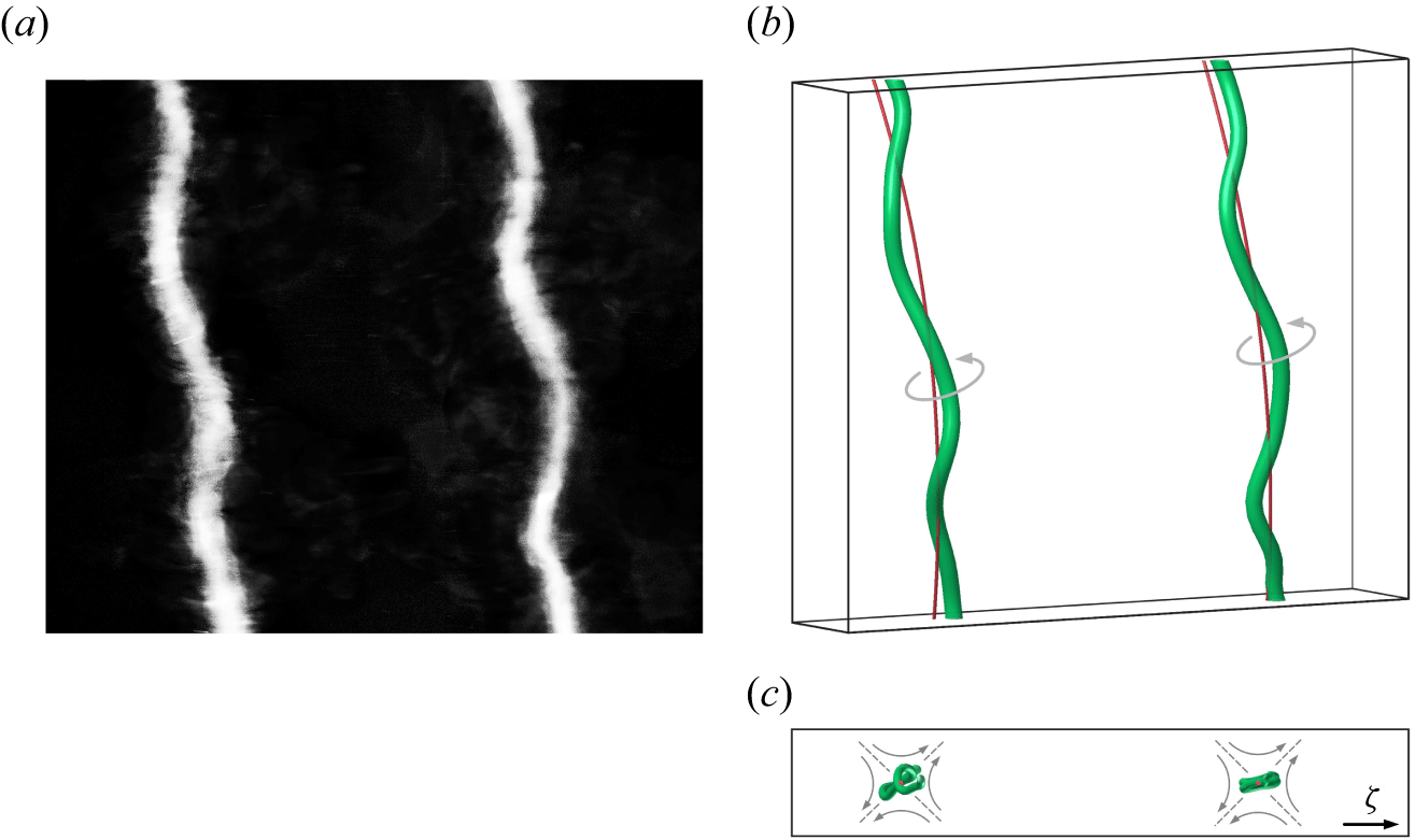
Perturbation structure for a forced wavenumber
 $M=16$
. (
 $a$
) Close-up dye visualisation in the region outlined in figure 2(
 $a$
). (
 $b$
) Three-dimensional reconstruction from stereoscopic images. The red line represents the axis of the unperturbed vortex. (
 $c$
) Axial view from below along the digitally straightened vortices of (
 $b$
). The mutually induced strain field is shown schematically in grey.

To isolate a single instability mode from these irregular waves, an additional experiment was conducted. The helical vortex was forced by periodically modulating the rotor rotation frequency
 $f$
with period
 $(Mf)^{-1}$
. Here, the number of waves per helix loop
 $M=L/\lambda$
is a measure for the instability scale, where
 $L=\sqrt {4\pi ^2R^2+h^2}$
is the length of one loop. The value of
 $M$
is determined by the choice of the target wavelength. In light of the results from the numerical stability analysis presented in § 4, two elliptic modes with wavenumbers
 $ka=0.47$
(
 $M=16$
) and
 $ka=1.61$
(
 $M=55$
) are candidates. Due to a limitation of the maximum motor bandwidth, perturbations with small
 $\lambda$
(large
 $k$
) are not experimentally accessible in our set-up. Therefore, the mode with
 $M=16$
is forced and becomes apparent closer to the rotor as a core displacement, with a well-defined wavelength matching the forcing. A close-up dye visualisation can be seen in figure 3(
 $a$
). Stereoscopic imaging from two viewing directions was used, in order to determine the three-dimensional structure of the vortex deformation, following Verhille & Bartoli (Reference Verhille and Bartoli2016). The reconstructed vortex lines are shown in figure 3(
 $b$
) for the unperturbed and perturbed cases. After digital straightening of the vortex axes, shown in figure 3(
 $c$
), the deformations of the vortex core are clearly visible. They are approximately planar, in a plane between the horizontal and the stretching direction of the strain field that the helix loops induce on each other. Classical elliptic instability is typically observed at much smaller wavelengths and involves more complex core perturbations than the apparent planar displacement of the vortex centre.
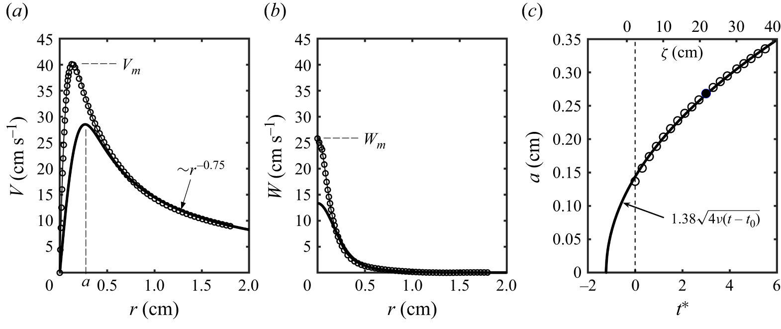
The properties of the tip vortex were determined from velocity measurements using stereoscopic PIV. Figures 4(
 $a$
) and 4(
 $b$
) present the radial profiles of swirl and axial velocity, respectively, at
 $\zeta /R_0=0.3$
. The measured profiles are close to the ones of the model proposed by Moore & Saffman (Reference Moore and Saffman1973) for trailing wing tip vortices. In particular, the swirl velocity approximately follows
 $r^{-0.75}$
for large distances
 $r$
, which implies that there is still significant axial vorticity in this region outside the viscous core, as illustrated by figure 5(
 $a$
). As indicated above, the core radius
 $a$
is here defined as the radial position of maximum swirl velocity
 $V_m$
. For the same configuration, Quaranta et al. (Reference Quaranta, Bolnot and Leweke2015) have reported a substantially larger value of
 $a$
, which was likely due to insufficient spatial resolution. The characteristics of the experimental helical vortex determined from visualisations and PIV are summarised in table 1. They also include the total circulation
 $\varGamma$
, determined using a circular contour of radius
 $h/2$
around the vortex centre, and the swirl number
 $S$
, defined as the ratio of maximum swirl to axial velocities.
As mentioned above, the wavelength of the unstable mode in figure 3 is significantly larger than that found for short-wave instabilities in other flows, which would typically have
 $M\gtrsim 50$
. It is also much smaller than the wavelengths of the pairing instability, which have
 $M=({1}/{2}), ({3}/{2}), ({5}/{2}), \ldots$
for the case of a single helix. In the next two sections, numerical simulation and stability analysis, as well as a theoretical considerations, will be used to further investigate this unexpected low-wavenumber short-wave displacement instability of a helical vortex.
Profiles of the mean azimuthally averaged (
 $a$
) swirl (
 $V$
) and (
 $b$
) axial (
 $W$
) velocity components of the tip vortex. Symbols represent the PIV measurements at
 $\zeta /R_0=0.3$
(
 $t^*=0$
), and the thick line the data at
 $t^*=3$
obtained from the numerical simulation. (
 $c$
) Temporal evolution of core size
 $a$
, from numerical simulation. The solid line gives the theoretical viscous evolution.

4. Numerical results
A direct numerical simulation (DNS) of the helical vortex was performed, initialised using experimental data, as explained in § 2.2. The truncated initial vorticity profile is shown qualitatively in figure 5(
 $a$
). Due to the small scale and moderate Reynolds number, the core radius increases significantly over the observation interval, as illustrated in figure 4(
 $c$
). When low-level white noise is initially added to trigger instability growth, short-wave perturbations appear in the helix (figure 5
 $b$
), with wavelengths and spiral structure resembling those observed in the (unforced) experiments (figure 2). Note that, while only a single helical loop is simulated, the image in figure 5
 $(b)$
(and those in figure 7 below) show multiple translated loops for clarity of interpretation.
(
 $a$
) Axial vorticity (
 $\eta$
) profile used for the numerical and theoretical analyses. The dashed line represents a Gaussian distribution. (
 $b$
) Visualisation from DNS (
 $Q$
-criterion, see Dubief & Delcayre Reference Dubief and Delcayre2000) of the short-wave instability at
 $t^*=6$
.

The frozen flow at
 $t^*=3$
, with the vortex velocity profiles shown as thick lines in figure 4(
 $a$
,
 $b$
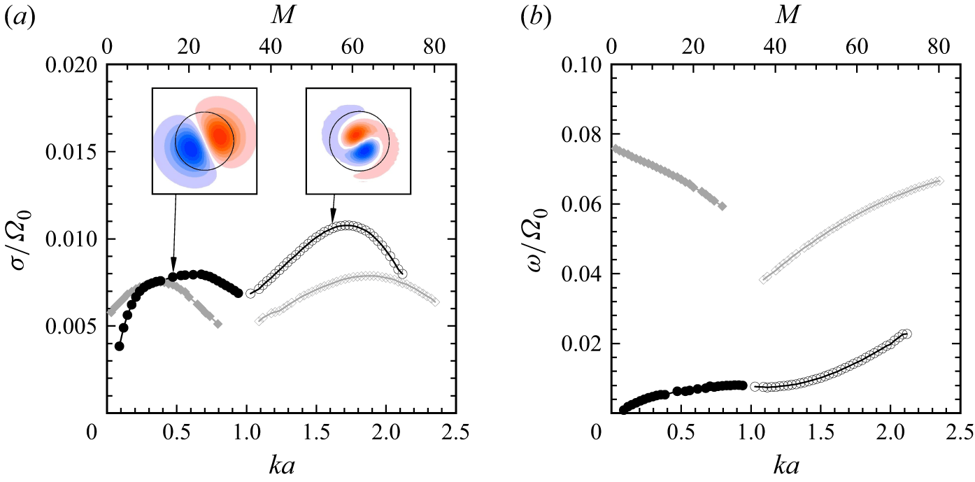
), was used for linear stability analysis. The results for the most unstable perturbations are given in figure 6. The growth rate (
 $\sigma$
) versus wavenumber
 $k$
(or equivalently
 $M$
) in figure 6(
 $a$
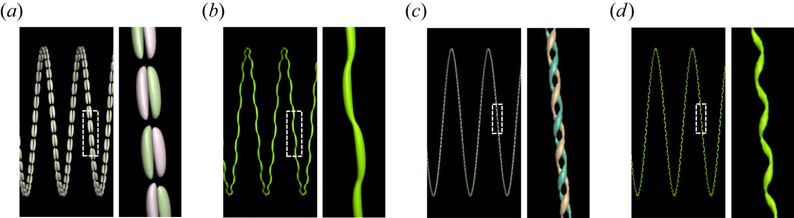
) presents four wide branches, illustrating a large range of unstable wavelengths. Representative mode structures are shown by cross-sectional perturbation vorticity, with three-dimensional views given in figure 7. At
 $ka=0.47$
, the perturbations consist of plane displacement waves of the vortex, whose orientation is similar to the experimental one for
 $M=16$
(figure 3). At larger
 $ka=1.61$
, the unstable modes take the form of higher-order helical bending modes, with a more complex core structure.
Numerical linear stability analysis of the helical vortex at
 $t^*=3$
. (
 $a$
) Growth rate of most unstable modes as a function of wavenumber, with corresponding perturbation vorticity in the vortex cross-section (the black circles have radius
 $a$
). Here,
 $\varOmega _0$
is the fluid angular velocity at the vortex centre. (
 $b$
) Frequencies of the modes shown in (
 $a$
), using the same symbols.

Structure of the unstable modes highlighted in figure 6(
 $a$
); (
 $a,b$
)
 $M=16, ka=0.47$
, (
 $c,d$
)
 $M=55, ka=1.61$
. Three-dimensional representation (and close-up) of (
 $a,c$
) azimuthal perturbation vorticity and (
 $b,d$
) total vorticity.

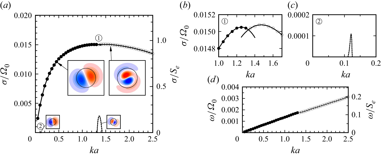
In order to further explore the origin of this instability, particularly the effect of vortex curvature, a second stability analysis was performed in the same way, for an array of straight parallel vortices with the same properties as in the helical case and spaced by the helix pitch
 $h$
. The result in figure 8 again shows a large interval of unstable wavenumbers, with basically the same unstable modes at small and large
 $k$
, and growth rates of the same order of magnitude. This similarity between the instabilities of the helical vortex and the straight-vortex array strongly suggests that vortex curvature is not at the origin of this phenomenon. The non-dimensional curvature, of order
 $a/R$
, is indeed quite small in our flow.
Numerical linear stability analysis of an array of straight vortices with the same velocity profiles and spacing as for the helical vortex. (
 $a$
) Growth rate as a function of wavenumber, with cross-sectional mode structures for
 $ka=0.45$
and
 $ka=1.60$
(large insets). The dashed lines correspond to the only unstable perturbations (small insets) arising from Kelvin mode resonances (branch crossings
 $C_1$
and
 $C_2$
in figure 9
 $b$
). (
 $b$
,
 $c$
) Enlargements of (
 $a$
). (
 $d$
) Mode frequencies.

In the following section, we use elements of short-wave instability theory to shed more light on the observations made from experiments and numerical simulation.
5. Theoretical results
Short-wavelength instabilities are usually associated with the resonance of modes of the underlying axisymmetric vortex with either the background strain field (elliptic instability) or corrections induced by vortex curvature (curvature instability). Since curvature can be ruled out here, the resonance would therefore be mediated by a strain field, implying a coupling between modes with azimuthal wavenumbers
 $m$
and
 $m+2$
. Both experimental and numerical results demonstrate that the instability involves modes with
 $|m|=1$
, which motivated us to focus on the vortex modes with azimuthal wavenumbers
 $m=1$
and
 $m=-1$
.
We use the underlying axisymmetric vortex profiles obtained from the numerical simulations at
 $t^*=3$
as the base flow. To isolate a single vortex, the axial vorticity decays smoothly to zero through a spline function for
 $r\gt h/2$
(figure 5
 $a$
), and the axial velocity is held constant beyond this radius. As explained in § 2.3, the vortex modes are obtained by solving the viscous linear stability problem. We compute Kelvin modes over a range of
 $k$
for azimuthal wavenumbers
 $m=1$
and
 $m=-1$
. The least-damped modes are selected in the calculation, because the instability is not expected when the modes have strong damping rates.
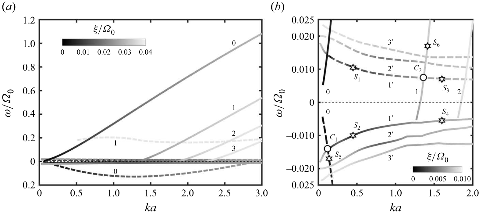
(
 $a$
) Dispersion relations for Kelvin modes of azimuthal wavenumbers
 $m=1$
(dashed lines) and
 $m=-1$
(solid lines) for a straight vortex with the same profile as the helical vortex at
 $t^*=3$
. The grey level indicates the damping rate. (
 $b$
) Close-up view around
 $\omega =0$
. The symbols marked
 $S_i$
refer to the mode structures shown in figure 10, and the
 $C_i$
refer to branch crossings.

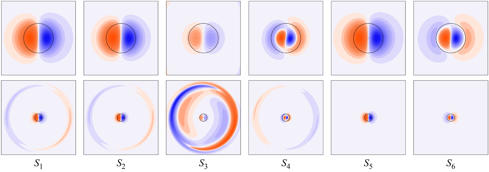
Structure of selected Kelvin modes identified in figure 9(
 $b$
). Top row: core region for
 $r/a\lt 2.5$
; bottom row: global view for
 $r/a\lt 10$
. The black circles have radius
 $a$
. Shown are:
 $S_1$
(
 $m=1$
,
 $n=1$
’,
 $ka=0.45$
);
 $S_2$
(−1, 1’, 0.45);
 $S_3$
(1, 1’, 1.60);
 $S_4$
(−1, 1’, 1.60);
 $S_5$
(1, 0, 0.14);
 $S_6$
(−1, 1, 1.42).

Figure 9(
 $a$
) presents the dispersion relation
 $\omega (k)$
, with the damping rate given by the grey level. Several branches labelled by
 $n$
are displayed for each
 $m$
. This label is related to the number of zeros of the radial velocity eigenfunction within the core (Sipp & Jacquin Reference Sipp and Jacquin2003) and provides a measure of the mode complexity. For
 $m=-1$
, the modes become increasingly damped as
 $n$
increases. For
 $m=1$
, two branches are obtained, for
 $n=0$
whose eigenmode has the same structure as that obtained for the
 $m=-1$
,
 $n=0$
branch, and for
 $n=1$
whose modes are much more damped. The spatial structures of the modes for typical branches
 $n=0$
and
 $n=1$
are illustrated in figure 10,
 $S_5$
and
 $S_6$
, respectively. The modes for the
 $n=0$
branches correspond to displacement modes.
Another family of eigenmodes is observed in the frequency range
 $-0.025\lt \omega \lt 0.025$
shown in figure 9(
 $b$
), where parts of the least-damped branches are displayed with special labels
 $1',2',3'$
. As with the classical branches, the modes become more strongly damped as
 $n$
increases. The spatial structures of these modes for
 $n=1'$
are shown in figure 10 (
 $S_1$
–
 $S_4$
) for the two axial wavenumbers corresponding to highlighted modes in the stability analysis. At small
 $k$
, the modes for
 $m=1$
and
 $m=-1$
are very similar, exhibiting the structure of the displacement mode within the core and a weak structure localised near the edge of the vortex at
 $r=h/2$
. As
 $k$
increases, the mode for
 $m=-1$
transitions within the vortex core to an
 $n=1$
mode, while for
 $m=1$
it remains a displacement mode, but with a stronger structure at the edge.
This family of eigenmodes is newly discovered here, it does not appear in standard vortex models. We computed the dispersion relation of an equivalent Batchelor vortex with identical core profiles (see below, figure 11) and only the expected classical branches were found. The modes of the new family seem to be associated with the weak vorticity present outside the vortex core (figure 5
 $a$
). The structure they exhibit at the edge is not associated with a critical layer, which lies much further away, in the region where the vortex is potential. Therefore, they are probably not critical-layer modes, such as the L2 family reported by Fabre et al. (Reference Fabre, Sipp and Jacquin2006) for the Lamb–Oseen vortex.
The
 $m=1$
and
 $m=-1$
branches intersect at several points (figure 9
 $b$
), where the corresponding modes can be resonantly coupled via the background strain field, making an elliptic instability possible, as explained in § 2.3. We computed the growth rates via the external strain rate
 $S_e$
for the array of straight vortices simulated above. The value of
 $S_e$
acting on a given vortex is obtained by superposing the strain field induced by all other vortices in the array. With one nearby vortex of circulation
 $\varGamma$
located at a distance
 $h$
, the induced strain rate is
 $\varGamma /(2\pi h^2)$
. The total contribution from the vortices on both sides of an infinite array is therefore
 \begin{equation} S_e = 2\boldsymbol{\cdot }\frac {\varGamma }{2\pi } \left ( \frac {1}{h^2} + \frac {1}{(2h)^2} + \frac {1}{(3h)^2} + {\cdots} \right ) = \frac {\pi \varGamma }{6h^2}. \end{equation}
The dimensionless strain rate for our configuration is
 $S_e/\varOmega _0=0.016$
.
(
 $a$
) Dispersion relations for Kelvin modes of azimuthal wavenumbers
 $m=1$
(dashed lines) and
 $m=-1$
(solid lines) for an equivalent Batchelor vortex, with the same core properties as the helical vortex at
 $t^*=3$
. The grey level indicates the damping rate. (
 $b$
) Close-up view around
 $\omega =0$
.

Previous work on the Lamb–Oseen vortex (Eloy & Le Dizès Reference Eloy and Le Dizès1999) and on a strained Batchelor vortex (Lacaze et al. Reference Lacaze, Ryan and Le Dizès2007; Roy et al. Reference Roy, Schaeffer, Le Dizès and Thompson2008) has demonstrated that resonances between modes with the same radial structure, i.e. with the same label
 $n$
for corresponding branches, are usually the most unstable. They are called ‘principal modes’. Among the resonant points, the sole principal mode for which the corresponding Kelvin modes share the same label
 $n=1$
was stable, because the mode for
 $m=1,n=1$
is too strongly damped. Only two resonances, denoted by
 $C_1$
and
 $C_2$
in figure 9(
 $b$
), were found to be unstable. However, their coupling coefficients are small due to the mismatch in radial structure. As a result, although
 $C_1$
and
 $C_2$
occur near the wavenumbers associated with the maximum amplification in the numerical stability analysis (figure 8), the resulting theoretical growth rates are approximately one order of magnitude lower than those predicted numerically. The mode resonance also cannot explain the large instability bands.
In order to further assess the role of classical resonances in our configuration, a stability analysis was performed with the same procedure for the equivalent Batchelor vortex, whose vorticity profile is shown in figure 5(
 $a$
) as a dotted line, and considering the same external strain (
 $S_e/\varOmega _0=0.016)$
. The growth rates of the resonances (branch crossings) in figure 11(
 $b$
) were computed exhaustively, but no unstable modes were found among them. This result is consistent with the one reported in figure 12(a) of Lacaze et al. (Reference Lacaze, Ryan and Le Dizès2007), where an instability map is presented for a similar strain rate
 $S_e/\varOmega _0=0.01$
. Our configuration falls outside the unstable regime. Therefore, the new instability cannot be explained by resonances between Kelvin modes from the classical branches.
We suspect that the instability arises from interaction between the new
 $n=1'$
branches for
 $m=1$
and
 $m=-1$
. Although these branches do not intersect, their frequencies remain close over a wide range of
 $k$
. A sufficiently strong strain field could then still couple these modes and induce growth that overcomes the damping associated with the weak frequency detuning between them. This mechanism would explain the structure of the unstable mode at
 $k=0.45$
, which corresponds to a superposition of the
 $m=1$
and
 $m=-1$
displacement modes with comparable amplitude, leading to a planar sinuous deformation of the vortex, as observed in figures 3 and 7(
 $a,b$
). At
 $k=1.60$
, the two
 $n=1'$
modes differ within the core, which would explain that their superposition forms a helical structure, possibly dominated by the structure of the
 $m=-1$
mode, in agreement with figure 7(
 $c,d$
).
A quantitative proof of this hypothesis is not provided here, because a numerically robust prediction of the growth rate between modes with special labels is beyond the present theoretical framework. In contrast to the classical resonances analysed above, this coupling has large contributions from regions far from the vortex core, where the elliptic correction is no longer a small perturbation. A new theoretical framework, valid up to the hyperbolic point, needs to be developed to correctly estimate this contribution.
6. Conclusions
We presented observations of a previously unexplored short-wave instability of a helical vortex generated by a rotor blade in a water channel, confirmed by numerical simulation of the same flow. A linear stability analysis, using the experimentally measured vortex profiles and geometry, reveals the existence of large wavenumber bands of unstable modes, characterised by planar or helical bending perturbations, which is a surprising result. In particular, a planar displacement mode is found for wavelengths much larger than for the classical elliptic instability, but also much smaller than for the well-known pairing instability. Stability results for an equivalent straight-vortex system show very similar features and rule out curvature as the source of the helical vortex instability. A new family of vortex perturbations (Kelvin modes) of azimuthal wavenumbers
 $m=\pm 1$
and low frequency is discovered, whose existence is linked to the particular velocity profile of the blade tip vortex, characterised by a region of low-level vorticity outside the inner viscous core. The experimental and numerical observations are consistent with the interaction of two of these modes, although the precise mechanism still needs to be determined, since their frequency branches never cross. The well-known mechanism of mode resonance through a strain field, which may lead to short-wave vortex instability, cannot account for the growth rates and unstable wavenumber bands found for the present flow configuration.
The structure of the new Kelvin modes bears similarities with certain instability modes of Stuart vortices, an analytical model of finite-core vortex arrays, for which a hyperbolic instability at the midpoints between vortices has been shown to play a role (Potylitsin & Peltier Reference Potylitsin and Peltier1999). The possible link with the Kelvin mode interaction considered here appears worthy of further investigation.
Acknowledgements
We thank G. Verhille for his help with the three-dimensional reconstruction of the helical vortex.
Funding
This work was supported by resources provided by the Pawsey Supercomputing Research Centre with funding from the Australian Government and the Government of Western Australia through NCMAS project d71. Z.X. received financial support from the China Scholarship Council (grant CSC 202406230291).
Declaration of interests
The authors report no conflict of interest.
 a
 b

 a
 ζ
 t∗
 ζ/R0=0.3
 b
 M=16
 a
 a
 b
 c
 b
 a
 V
 b
 W
 ζ/R0=0.3
 t∗=0
 t∗=3
 c
 a
 a
 η
 b
 Q
 t∗=6
 t∗=3
 a
 a
 Ω0
 b
 a
 a
 a,b
 M=16,ka=0.47
 c,d
 M=55,ka=1.61
 a,c
 b,d
 a
 ka=0.45
 ka=1.60
 C1
 C2
 b
 b
 c
 a
 d
 a
 m=1
 m=−1
 t∗=3
 b
 ω=0
 Si
 Ci
 b
 r/a<2.5
 r/a<10
 a
 S1
 m=1
 n=1
 ka=0.45
 S2
 S3
 S4
 S5
 S6

 a
 m=1
 m=−1
 t∗=3
 b
 ω=0

 Open access

