1 Introduction and the drag reduction mechanism

The use of complex surfaces to reduce skin friction drag has been an active area of scientific interest for several decades. Superhydrophobic surfaces have recently attracted a growing amount of research into their drag reduction capabilities. These surfaces combine chemical hydrophobicity with surface micro-roughness. This combination allows pockets of gas to be entrapped in between the roughness elements when the surfaces are submerged in water (Rothstein Reference Rothstein2010). Drag reduction can result from the overlying flow locally slipping over the effective surface formed by the roughness crests and entrapped gas pockets, as sketched in figure 1, giving a mean slip velocity at this effective surface. This drag reduction potential has been realised under experimental conditions, in both laminar (Watanabe, Udagawa & Udagawa Reference Watanabe, Udagawa and Udagawa1999; Ou, Perot & Rothstein Reference Ou, Perot and Rothstein2004), and turbulent flows (Daniello, Waterhouse & Rothstein Reference Daniello, Waterhouse and Rothstein2009; Woolford et al. Reference Woolford, Prince, Maynes and Webb2009) and has been demonstrated in idealised numerical simulations (Min & Kim Reference Min and Kim2004; Martell, Perot & Rothstein Reference Martell, Perot and Rothstein2009).

Figure 1.

Schematic of flow over a submerged superhydrophobic surface showing the regions of no slip and free slip over the roughness elements and entrapped gas pockets respectively.

The performance of superhydrophobic surfaces can be characterised through the concept of slip lengths. By considering the mean velocity at the surface, a slip length is introduced through the Navier slip condition (Navier Reference Navier1823), defined as

(1.1) $$\begin{eqnarray}u_{s}=\ell _{x}\left|\frac{\unicode[STIX]{x2202}u}{\unicode[STIX]{x2202}y}\right|_{s},\end{eqnarray}$$

where the slip velocity, $u_{s}$ , is the mean velocity at the surface, $|\unicode[STIX]{x2202}u/\unicode[STIX]{x2202}y|_{s}$ is the mean wall-normal velocity gradient at the surface and $\ell _{x}$ is the mean slip length. This slip length defines the virtual origin experienced by the mean flow, i.e. it is the distance below the surface where the mean flow would experience a non-slipping wall. The value of the slip length depends on the geometry and size of the surface texture. Analytical solutions for the slip length have been derived for textures of streamwise and spanwise aligned ridges in the viscous Stokes regime (Philip Reference Philip1972; Lauga & Stone Reference Lauga and Stone2003) and have been obtained numerically for textures of regular arrays of isolated posts in the same regime (Ybert, Barentin & Cottin-Bizonne Reference Ybert, Barentin and Cottin-Bizonne2007). The slip lengths obtained in the viscous regime have been shown to hold in turbulent flows for small texture sizes, $L^{+}\lesssim 10$ (Seo & Mani Reference Seo and Mani2016), where $L$ is the texture spacing, as shown in figure 1, and the $+$ superscript denotes scaling in wall units. For larger $L^{+}$ , the slip length deviates from the viscous prediction. Seo & Mani (Reference Seo and Mani2016) attributed this deviation to the development of boundary layers over the roughness elements. They proposed a model, for sufficiently large texture sizes, $L^{+}\sim 100$ , where the slip length scales with the cube root of the texture size. A physical model for the slip length in between the Stokes regime and the model proposed by Seo & Mani (Reference Seo and Mani2016) is, however, still missing. We conduct laminar simulations, shown in figure 2, and compare the obtained slip lengths to our direct numerical simulation (DNS) results taken from later in this paper. The laminar simulations are able to capture the initial deviation from the viscous prediction, which suggests that the initial deviation is due to advective effects. However, these laminar simulations fail to predict the slip length beyond $L^{+}\gtrsim 20$ , where the slip length tends to the relation proposed by Seo & Mani (Reference Seo and Mani2016).

For laminar flows, drag reduction using superhydrophobic surfaces depends only on the value of the slip length in the streamwise direction, $\ell _{x}$ , which acts to shift the mean velocity profile by the slip velocity. In turbulent flows, however, the spanwise slip length, $\ell _{z}$ , also influences the surface drag (Min & Kim Reference Min and Kim2004). As shown by Luchini (Reference Luchini2015), this is analogous to the drag reduction mechanism of riblets, where drag reduction was shown to be proportional to the difference between the streamwise and spanwise slip lengths (Luchini, Manzo & Pozzi Reference Luchini, Manzo and Pozzi1991; Luchini Reference Luchini1996), or protrusion heights in riblet terminology. The effect of spanwise slip has been attributed to allowing quasi-streamwise vortices, part of the near-wall turbulent cycle, to move closer to the surface (Min & Kim Reference Min and Kim2004; Luchini Reference Luchini2015).

Figure 2.

Variation of the slip length with texture size: - - - -, Stokes-flow prediction (Ybert et al. Reference Ybert, Barentin and Cottin-Bizonne2007); –○–, laminar simulations; –▫–, streamwise slip length $\ell _{x}^{+}$ from the present study (DNS); –▵–, spanwise slip length $\ell _{z}^{+}$ from the present study; –♢–, $\ell _{z,eff}^{+}$ from (1.5) for the previous $\ell _{z}^{+}$ values.

For small surface manipulations, the classical theory of wall turbulence states that the only influence of the surface on the outer flow is the location at which the outer flow perceives the wall. With drag-reducing surfaces, the logarithmic region of the mean velocity profile, $U^{+}$ , is shifted upwards, and with drag increasing surfaces it is shifted downwards. The Kármán constant, $\unicode[STIX]{x1D705}$ , and wake function remain unmodified (Clauser Reference Clauser1956). It follows that the free-stream velocity, $U_{\unicode[STIX]{x1D6FF}}^{+}$ , of a surface with small sized manipulations, can be given by

(1.2) $$\begin{eqnarray}U_{\unicode[STIX]{x1D6FF}}^{+}=\left(\frac{2}{c_{f}}\right)^{1/2}=\unicode[STIX]{x1D705}^{-1}\log \unicode[STIX]{x1D6FF}^{+}+B+\unicode[STIX]{x0394}U^{+},\end{eqnarray}$$

where $c_{f}$ is the skin friction coefficient, $\unicode[STIX]{x0394}U^{+}$ is the difference of the mean velocity profile compared to a smooth wall far enough from the surface, $\unicode[STIX]{x1D6FF}^{+}$ is the flow thickness and $B$ includes the smooth-wall logarithmic intercept and the wake function. When considering a boundary layer, $\unicode[STIX]{x1D6FF}$ is the boundary-layer thickness. For a channel $\unicode[STIX]{x1D6FF}$ is the channel half-height, with $U_{\unicode[STIX]{x1D6FF}}^{+}$ the channel centreline velocity. Defining the friction coefficient, $c_{f}$ , based on $U_{\unicode[STIX]{x1D6FF}}$ , from (1.2), a relation between $\unicode[STIX]{x0394}U^{+}$ and the drag reduction can be obtained. Compared to a smooth wall at the same $\mathit{Re}_{\unicode[STIX]{x1D70F}}$ , we have

(1.3) $$\begin{eqnarray}DR=-\frac{\unicode[STIX]{x0394}c_{f}}{c_{f_{0}}}=1-\frac{1}{\left(1+\unicode[STIX]{x0394}U^{+}/U_{\unicode[STIX]{x1D6FF}_{0}}^{+}\right)^{2}},\end{eqnarray}$$

where $c_{f_{0}}$ and $U_{\unicode[STIX]{x1D6FF}_{0}}^{+}$ are the skin friction coefficient and free-stream velocity for the reference smooth wall. As $U_{\unicode[STIX]{x1D6FF}_{0}}^{+}$ , and $c_{f_{0}}$ , are weakly dependent on the Reynolds number, if $Re_{\unicode[STIX]{x1D70F}}=\unicode[STIX]{x1D6FF}^{+}$ differs between the two cases an additional logarithmic correction to (1.3) is required (Gatti & Quadrio Reference Gatti and Quadrio2016). For riblets of small size, it was shown that $\unicode[STIX]{x0394}U^{+}$ varies linearly with the difference between the streamwise and spanwise slip lengths (Luchini et al. Reference Luchini, Manzo and Pozzi1991; Luchini Reference Luchini1996). That is,

(1.4) $$\begin{eqnarray}\unicode[STIX]{x0394}U^{+}=\unicode[STIX]{x1D707}_{0}~(\ell _{x}^{+}-\ell _{z}^{+}),\end{eqnarray}$$

where $\unicode[STIX]{x1D707}_{0}$ is a coefficient of order unity (Jiménez Reference Jiménez1994; Luchini Reference Luchini1996; Bechert et al. Reference Bechert, Bruse, Hage, van der Hoeven and Hoppe1997). For superhydrophobic surfaces, this relationship for $\unicode[STIX]{x0394}U^{+}$ holds when the spanwise slip length is small. However, as the spanwise slip length increases, the effect of spanwise slip on $\unicode[STIX]{x0394}U^{+}$ saturates (Fukagata, Kasagi & Koumoutsakos Reference Fukagata, Kasagi and Koumoutsakos2006). A parametric study was carried out by Busse & Sandham (Reference Busse and Sandham2012), which mapped the obtained drag reduction for a range of streamwise and spanwise slip lengths. Their results are consistent with the spanwise effect being governed by an ‘effective’ spanwise slip length, $\ell _{z,eff}^{+}$ (Fairhall & García-Mayoral Reference Fairhall and García-Mayoral2018), given by

(1.5) $$\begin{eqnarray}\ell _{z,eff}^{+}=\frac{\ell _{z}^{+}}{1+\ell _{z}^{+}/4},\end{eqnarray}$$

and the velocity shift is then,

(1.6) $$\begin{eqnarray}\unicode[STIX]{x0394}U^{+}\approx \ell _{x}^{+}-\ell _{z,eff}^{+},\end{eqnarray}$$

with the coefficient $\unicode[STIX]{x1D707}_{0}\approx 1$ , as proposed by Luchini (Reference Luchini1996, Reference Luchini2015). García-Mayoral, Gómez-de-Segura & Fairhall (Reference García-Mayoral, Gómez-de-Segura and Fairhall2018) argue that if the dynamics of turbulence is unaltered except for a wall-normal shift then $\unicode[STIX]{x1D707}_{0}$ must necessarily be equal to 1. Preliminary analysis in Gómez-de-Segura et al. (Reference Gómez-de-Segura, Fairhall, MacDonald, Chung and García-Mayoral2018) suggests that the cause of the saturation effect of $\ell _{z}^{+}$ results from the impermeability imposed at the surface, an effect not present with riblets. The imposed impermeability acts to limit the shift of quasi-streamwise vortices towards the surface. Therefore, to maximise drag reduction for any surface modification, the streamwise slip length should be maximised, and the spanwise slip length and the wall-normal permeability minimised.

With real superhydrophobic surfaces, the liquid–gas interface of the gas pockets is able to deform in response to the overlying flow. This has the effect of relaxing the impermeability condition of the wall-normal velocity fluctuations. Seo, García-Mayoral & Mani (Reference Seo, García-Mayoral and Mani2018) included coupling of the gas pocket deformation with the overlying turbulent flow in their numerical simulations. They found that, compared to simulations where the gas pockets were considered rigid, the mean velocity profile and turbulent fluctuations appear to remain essentially unmodified when the liquid–gas interface is free to deform, for texture sizes up to $L^{+}\lesssim 30$ . The similarity between the mean velocity profiles and the velocity fluctuations of deformable and undeformable surfaces reported in their work suggests that the shift of turbulence closer to the surface, due to spanwise slip, is not further increased by the relaxation of the impermeability of wall-normal velocity fluctuations, at least for $L^{+}\lesssim 30$ .

From (1.6), to maximise drag reduction the streamwise slip length should be maximised. Increasing the texture size is one way to increase the slip length (Philip Reference Philip1972; Ybert et al. Reference Ybert, Barentin and Cottin-Bizonne2007). However, increasing the texture size eventually leads to the loss of the gas pockets from the surface. The surface then becomes a rough surface, potentially increasing the drag. One possible cause for this is due to pressure fluctuations deforming the gas pockets, which eventually overcome the surface tension keeping them entrapped. Seo, García-Mayoral & Mani (Reference Seo, García-Mayoral and Mani2015) reported a texture-coherent pressure deformation distribution, caused by stagnation of the slipping flow at the texture elements. Seo et al. (Reference Seo, García-Mayoral and Mani2018) found that, for $L^{+}\gtrsim 30$ , an upstream-travelling capillary wave of the interface can develop for sufficiently large Weber numbers, whose onset significantly increased the pressure fluctuations. Both of these mechanisms increase pressure fluctuations with increasing texture size, and are possible explanations for the failure mechanism of superhydrophobic surfaces. An alternative potential cause for the loss of the gas pockets is the shear driven failure mechanism (Wexler et al. Reference Wexler, Grosskopf, Chow, Fan, Jacobi and Stone2015a ; Wexler, Jacobi & Stone Reference Wexler, Jacobi and Stone2015b ) in which the lubricating fluid is depleted due to shear with the overlying flow. This failure mechanism is more prevalent with liquid infused surfaces, where a liquid is used as the lubricating fluid rather than air (Lafuma & Quere Reference Lafuma and Quere2011; Wong et al. Reference Wong, Kang, Tang, Smythe, Hatton, Grinthal and Aizenberg2011). With these surfaces, there is a smaller disparity in viscosity between the lubricating fluid and the overlying fluid, and consequently a larger interfacial shear compared to superhydrophobic surfaces.

Predicting the performance of surfaces using slip lengths assumes that the size of the surface texture is small compared to the scales in the overlying turbulent flow (Bechert & Bartenwerfer Reference Bechert and Bartenwerfer1989). In this theoretical ‘vanishingly small’ limit, the overlying turbulent structures only experience the surface through the averaged effect of the texture, i.e. its slip lengths. They do not perceive individual texture elements. Slip-length boundary conditions were used in early DNS studies of superhydrophobic surfaces to predict the attainable drag reduction (Min & Kim Reference Min and Kim2004; Busse & Sandham Reference Busse and Sandham2012). Slip-length models are attractive in computational simulations because additional spatial resolution is not required to resolve the flow around the texture elements. However, as the texture size becomes of the order of turbulent structures in the overlying flow, the assumption of vanishing texture size becomes inappropriate. Consequently, the majority of recent simulations of superhydrophobic surfaces explicitly resolve the surface texture (Martell et al. Reference Martell, Perot and Rothstein2009; Park, Park & Kim Reference Park, Park and Kim2013; Jelly, Jung & Zaki Reference Jelly, Jung and Zaki2014; Türk et al. Reference Türk, Daschiel, Stroh, Hasegawa and Frohnapfel2014; Rastegari & Akhavan Reference Rastegari and Akhavan2015; Seo et al. Reference Seo, García-Mayoral and Mani2015; Fairhall & García-Mayoral Reference Fairhall and García-Mayoral2018).

Seo & Mani (Reference Seo and Mani2016) investigated the applicability of modelling textured surfaces using slip lengths. They compared the results from simulations where the texture geometry was resolved to ones with equivalent homogeneous slip lengths, obtained from the texture-resolved simulations. To assess the validity of the slip-length model, they measured the instantaneous slip lengths of individual texture elements and compared these values to the measured slip length of the mean flow. They found that for small textures, in their case $L^{+}\lesssim 10$ , the instantaneous slip length experienced by individual texture elements was close to the measured slip length of the mean flow, with the mean velocity profiles of both surface representations matching. For larger textures, however, the velocity and shear over individual texture elements appeared to lose correlation, resulting in large variations in the instantaneous slip lengths. A large disagreement was also present between the obtained mean velocity profiles from the two surface representations when correlation was lost.

Fairhall & García-Mayoral (Reference Fairhall and García-Mayoral2018) further investigated the validity of slip-length models in texture-resolved simulations. They analysed the boundary condition experienced by length scales of the overlying turbulence that are much larger than the texture size, using a Fourier approach to discriminate between different length scales. They showed that even scales much larger than the texture size displayed an apparent loss of correlation, not just scales of the order of the texture size. They proposed that this observed loss of correlation was due to the magnitude of the texture-induced flow becoming of the order of the overlying turbulent flow, contaminating the perceived slip length, rather than a direct effect of the texture size becoming too large.

The separate effects that slip and surface texture have on the overlying turbulence are also not completely clear. The results of Min & Kim (Reference Min and Kim2004) and Busse & Sandham (Reference Busse and Sandham2012), which model the surface through homogeneous slip lengths, show both a shift of the peaks of the root mean square (r.m.s.) of fluctuations and a change in their magnitudes. They suggest that slipping surfaces both shift turbulence closer to the surface and modify the intensity of the near-wall turbulent cycle. However, both these simulations were conducted with a constant mass flow rate and present their results normalised by the friction velocity of the smooth wall reference case. As the simulations produce either a drag reduction or a drag increase, due to the imposed constant mass flow rate, the actual friction velocity for each individual case changes. Scaling by the smooth-wall friction velocity therefore artificially modifies the magnitudes of the peaks of the fluctuations, potentially contributing to the change of turbulence intensity observed. Simulations in a channel with superhydrophobic boundary conditions applied to only one wall have also been observed to display a shift and weakening of turbulent fluctuations near the superhydrophobic surface (Martell et al. Reference Martell, Perot and Rothstein2009). However, in this non-symmetric set-up, there is no clearly defined friction Reynolds number, which makes it difficult to assess what effects the superhydrophobic surface has on the overlying turbulence.

Previous studies have also investigated the interaction of the surface texture elements with the overlying turbulent flow. In numerical simulations of textured surfaces, formed by streamwise aligned grooves, Jelly et al. (Reference Jelly, Jung and Zaki2014) and Türk et al. (Reference Türk, Daschiel, Stroh, Hasegawa and Frohnapfel2014) showed that, for sufficiently large texture sizes, additional secondary and tertiary flows are generated by the alternating no-slip/free-slip nature of the surface, which act to increase the drag. The results of the numerical simulations of Rastegari & Akhavan (Reference Rastegari and Akhavan2015) and Seo et al. (Reference Seo, García-Mayoral and Mani2015) also show that the presence of surface texture can significantly modify turbulent fluctuations near the surface. Busse & Sandham (Reference Busse and Sandham2013) included the effect of the roughness elements protruding into the flow in their numerical simulations. They showed that the drag-reducing effect of slip can be eliminated by the additional drag from the exposed roughness elements. Experimental studies have also observed that for sufficiency large roughness size, expressed in wall units, superhydrophobic surfaces resulted in a drag increase rather than a drag decrease. This has been attributed to the protrusion of roughness elements introducing additional drag and roughness-like effects (Bidkar et al. Reference Bidkar, Leblanc, Kulkarni, Bahadur, Ceccio and Perlin2014; Ling et al. Reference Ling, Srinivasan, Golovin, McKinley, Tuteja and Katz2016; Gose et al. Reference Gose, Golovin, Boban, Mabry, Tuteja, Perlin and Ceccio2018). Ling et al. (Reference Ling, Srinivasan, Golovin, McKinley, Tuteja and Katz2016) also investigated the effect of increasing the roughness protrusion, for the same texture, by increasing the overlying fluid pressure in their experiments. Their results showed an increase in drag with increasing fluid pressure as the roughness elements are increasingly exposed.

In this work we reassess the applicability of slip-length models for textured superhydrophobic surfaces by isolating the slip length experienced by the overlying turbulence. We then analyse the effects of surface slip and surface texture separately. The paper is organised as follows. Section 2 outlines the numerical method we use. In § 3 we use a modified form of the triple decomposition (Abderrahaman-Elena & García-Mayoral Reference Abderrahaman-Elena and García-Mayoral2016; Abderrahaman-Elena, Fairhall & García-Mayoral Reference Abderrahaman-Elena, Fairhall and García-Mayoral2019) to isolate the overlying turbulent flow from the texture-induced flow and reassess the apparent slip length. We then analyse the results from equivalent slip-length simulations in § 4, and compare these to texture-resolving simulations in § 5, to determine the effects of slip and texture separately. Our findings are then summarised in § 6.

2 Numerical method

Two sets of direct numerical simulations (DNS) of turbulent channels were conducted. The first set of simulations resolve the surface texture geometry, by applying alternating free-slip and no-slip boundary conditions to both channel walls. The gas pockets are considered rigid, resulting in an impermeability condition at the surface. The use of a free-slip boundary condition neglects all dynamics of the flow within the gas pockets. Schonecker, Baier & Hardt (Reference Schonecker, Baier and Hardt2014) investigated the effect of coupling the lubricating fluid with the overlying flow on the obtained slip length. They showed that while the free-slip condition over-predicts the slip length, it can give a reasonable model provided that the gas pockets are sufficiently deep. Seo et al. (Reference Seo, García-Mayoral and Mani2018) showed that for texture sizes reported in experimental studies, $L^{+}\lesssim O(10)$ (Daniello et al. Reference Daniello, Waterhouse and Rothstein2009; Woolford et al. Reference Woolford, Prince, Maynes and Webb2009; Bidkar et al. Reference Bidkar, Leblanc, Kulkarni, Bahadur, Ceccio and Perlin2014; Ling et al. Reference Ling, Srinivasan, Golovin, McKinley, Tuteja and Katz2016; Rosenberg et al. Reference Rosenberg, Buren, Fu and Smits2016; Gose et al. Reference Gose, Golovin, Boban, Mabry, Tuteja, Perlin and Ceccio2018), the interface deformation should be small. Their results showed for textures of this size, the turbulent velocity fluctuations were essentially unmodified by the inclusion of interface deformation.

Figure 3.

Instantaneous realisation of vortical structures, represented using the Q-criterion, showing the surface texture for the case with $L^{+}\approx$ 47.

The surface texture considered in our simulations consists of a regular array of square posts in a collocated arrangement, as shown in figure 3, with a solid fraction, the ratio of post area to total surface area, $\unicode[STIX]{x1D719}_{s}=1/9$ . In experimental studies $L$ is typically kept fixed while the Reynolds number is varied between experiments. As a result, $u_{\unicode[STIX]{x1D70F}}$ and therefore $L^{+}$ changes. Here we adopt the typical DNS approach of keeping the Reynolds number and $u_{\unicode[STIX]{x1D70F}}$ approximately constant between simulations and changing $L$ , so an equivalent parametric sweep for $L^{+}$ is achieved. The texture spacings we consider range from $L^{+}\approx 6$ to 47, and are listed in table 1. The simulations with $L^{+}\approx 12$ , 24, and 47 were previously reported in Fairhall & García-Mayoral (Reference Fairhall and García-Mayoral2018). The second set of simulations replace the textured surfaces by the slip lengths, obtained a posteriori from the texture-resolved simulations, and are also listed in table 1.

Table 1.

Simulation parameters for the textured and homogeneous slip-length simulations. $L^{+}$ is the texture size in wall units, or the texture size for which the applied slip lengths are equivalent. $Re_{\unicode[STIX]{x1D70F}_{\unicode[STIX]{x1D6FF}}}$ is the friction Reynolds number. $N_{x,w}$ and $N_{z,w}$ are the number of grid points in the streamwise and spanwise directions in the refined blocks near the channel walls, with $n_{x}$ and $n_{z}$ the number of grid points per texture element in the refined block for the streamwise and spanwise directions respectively. $N_{y}$ is the number of grid points in the wall-normal direction. $\overline{\ell }_{x}^{+}$ is the mean slip length, $\widehat{\ell }_{x}$ and $\widehat{\ell }_{z}$ are the dynamic slip lengths and $\unicode[STIX]{x0394}U^{+}$ is the resulting shift of the logarithmic region of the mean velocity profile.

The numerical code has been adapted from García-Mayoral & Jiménez (Reference García-Mayoral and Jiménez2011) and is briefly summarised here. Further numerical details are given in Fairhall & García-Mayoral (Reference Fairhall and García-Mayoral2018). The three-dimensional incompressible Navier–Stokes equations are solved using a spectral discretisation in the streamwise ( $x$ ) and spanwise ( $z$ ) directions with the wall-normal ( $y$ ) direction discretised using second-order finite differences on a staggered grid. A fractional step method is used (Kim & Moin Reference Kim and Moin1985), combined with a three-step Runge–Kutta to advance in time with a semi-implicit scheme used for the viscous terms and an explicit scheme for the advective terms (Le & Moin Reference Le and Moin1991). The advective terms are dealiased using the ‘ $2/3$ rule’. All simulations were run at a friction Reynolds number, $Re_{\unicode[STIX]{x1D70F}_{\unicode[STIX]{x1D6FF}}}=180$ , based on the channel half-height, $\unicode[STIX]{x1D6FF}$ , by applying a constant mean pressure gradient. The channel is of size $2\unicode[STIX]{x03C0}\unicode[STIX]{x1D6FF}\times \unicode[STIX]{x03C0}\unicode[STIX]{x1D6FF}\times 2\unicode[STIX]{x1D6FF}$ in the streamwise, spanwise and wall-normal directions respectively.

Figure 4.

Difference between (a) mean velocity profiles, with slip velocity ( $u_{s}$ ) subtracted; (b) r.m.s. velocity fluctuations; (c) wall-normal decay of streamwise coherent flow for the DNS grid resolution dependency test with $L^{+}\approx 24$ . Lines: - - - -, smooth wall; –▫–, 12 points per texture; –○–, 24 points per texture; –♢–, 36 points per texture; –▵– 48 points per texture.

Figure 5.

Comparison of the spectral energy densities of the three velocities and Reynolds stress at $y^{+}=15$ for the cases with $L^{+}\approx 24$ of the DNS grid resolution dependency test. Filled contour, 12 points per texture; —— 24 points per texture; - - - - 36 points per texture.

Figure 6.

Dependency of the mean streamwise slip length with grid resolution in viscous Stokes-flow simulations. Lines: –○–, finite difference discretisation; –▫–, spectral discretisation; –♢–, error of DNSs assuming that the error with 48 points per texture element matches the Stokes-flow error.

To reduce the computational cost of the texture-resolved simulations, the code uses a ‘multiblock’ grid which allows finer resolution near the walls, taking the form of additional Fourier modes, compared to the channel centre (García-Mayoral & Jiménez Reference García-Mayoral and Jiménez2011). The grid resolution in the channel centre, and for the homogeneous slip-length simulations, is $\unicode[STIX]{x0394}x^{+}\approx 8.8$ , $\unicode[STIX]{x0394}z^{+}\approx 4.4$ with $\unicode[STIX]{x0394}y_{min}^{+}\approx 0.3$ at the surfaces and $\unicode[STIX]{x0394}y_{max}^{+}\approx 3$ in the channel centre. For the texture-resolved simulations, the grid resolution near the surface is dependent on the texture size to obtain sufficient resolution of the flow around the texture elements. For the cases with $L^{+}\approx 18$ to 47, all results reported use 24 grid points per texture element. For the case with $L^{+}\approx 12$ , due to the computational cost, 12 grid points per texture element are used for the turbulent statistics. To assess the effects of this different grid resolution, the case with $L^{+}\approx 24$ was also run with 12, 36 and 48 points per texture element. The turbulent statistics with 12, 24 and 36 grid points per texture show good agreement, as shown in figure 4, suggesting that the overlying turbulence is not affected by the grid resolution. This is further supported by the respective premultiplied energy spectra, as shown at $y^{+}=15$ in figure 5, which show negligible change to the distribution of turbulent energy with varying grid resolution. Additionally, the r.m.s. of the ensemble-averaged texture-coherent flow with 12 points per texture element is within 4 % of the value with 48 points per texture element, as shown in figure 4(c), suggesting only a weak influence of the resolution on the texture-induced flow. There is, however, a discrepancy in the value of the mean slip length between both grid resolutions. To investigate this discrepancy, we conducted viscous Stokes-flow simulations for varying grid resolutions. The Stokes-flow code uses the same fractional step scheme as the DNS code, but with the viscous term solved using a fully implicit method. The domain size is $L\times L\times 4L$ , with the flow driven by a homogeneous shear at $y=4L$ . A comparison of the grid dependency for a collocated, spectral discretisation and a staggered, finite-difference discretisation is shown in figure 6. Both simulation set-ups converge to the same value of the mean slip length with increasing grid resolution. The spectral discretisation, however, converges at a slower rate. For the spectral discretisation with 24 grid points per texture element, the difference of the obtained slip length, when compared to a staggered finite-difference discretisation with 72 points, is 14 %. Using 12 points per texture, the difference is 27 %. The error from DNSs with the same resolutions is portrayed superimposed in the figure, assuming that the error for 48 points per texture is the same to set a common scale. The similar trend between the Stokes flow and DNS convergence suggests that the error in the DNSs is consistent with that of the Stokes-flow simulations, which suggests that the slip lengths obtained from DNS can be corrected by the Stokes-flow error to offset this resolution dependency. Note nevertheless that this error only affects the mean slip length, and therefore the offset of the mean velocity profile, but it does not affect the turbulent fluctuations or the texture-coherent flow.

Figure 7.

Ratio of the DNS streamwise slip lengths (with spectral discretisation) to the Stokes-flow slip lengths with finite-difference discretisation: ●, 24 points per texture; ▪, 12 points per texture; ♦, 36 points per texture; ▾, 48 points per texture. The results at $L^{+}=0$ are obtained from the viscous Stokes-flow simulations. The solid symbols represent the actual slip lengths obtained from the simulations. The hollow symbols show the estimated grid-converged slip lengths obtained from assuming the discretisation error is the same in the Stokes-flow simulations and the DNSs. ▵, results from Seo & Mani (Reference Seo and Mani2016).

Figure 8.

Validation of the implementation of the free-slip/no-slip boundary conditions versus the case with $L^{+}\approx 39$ from Seo et al. (Reference Seo, García-Mayoral and Mani2015). (a) Mean velocity profiles, with slip velocity ( $u_{s}$ ) subtracted; (b) r.m.s. velocity fluctuations: – –, smooth wall; ——, present results; ○, results from Seo et al. (Reference Seo, García-Mayoral and Mani2015).

The obtained streamwise slip lengths from the DNSs, together with the Stokes-flow slip lengths in the viscous limit, $L^{+}\ll 1$ , and results from Seo & Mani (Reference Seo and Mani2016) are shown in figure 7. By assuming again that the discretisation error of the DNSs is the same as the discretisation error of the viscous Stokes-flow simulations, with the same spectral discretisation, estimates of the grid-converged DNS slip lengths are obtained. For different grid resolutions, the estimated slip lengths for the same texture size have similar values and are close to the slip lengths obtained by Seo & Mani (Reference Seo and Mani2016). This further indicates that the discretisation error of the DNSs is consistent with the discretisation error of the Stokes-flow simulations. Due to this grid-resolution dependency, and to allow a fair comparison of the slip-length statistics between texture sizes, the case with $L^{+}\approx 12$ was further run with 24 points per texture element until the texture-coherent statistics had converged. The texture-coherent statistics have a much shorter time scale than the statistics for the overlying turbulence so they could be obtained at a more moderate cost. All statistics presented for the slip lengths in the results and subsequent analysis are obtained from the simulation with 24 points per texture. To obtain the texture-coherent slip lengths and statistics for $L^{+}\approx 6$ , we conducted an additional simulation using the laminar slip-lengths, shown in figure 2, as initial conditions. The implementation of the boundary conditions was validated against the case with $L^{+}\approx 39$ of Seo et al. (Reference Seo, García-Mayoral and Mani2015), as shown in figure 8. It should be noted that the grid resolution dependency of the spectral code suggests that the slip lengths in the present work are consistently under-predicted, compared to previous work in the literature where finite-difference discretisations were used. This is demonstrated in the slight mismatch between the mean velocity profile compared to Seo et al. (Reference Seo, García-Mayoral and Mani2015) in figure 8. However, the actual values of the slip lengths are not the focus of the present work, and the turbulent statistics on the other hand appear to agree well.

2.1 Effect of Reynolds number

To investigate any dependence on the Reynolds number, additional simulations of the cases with $L^{+}\approx 24$ and $L^{+}\approx 35$ were conducted at $Re_{\unicode[STIX]{x1D70F}}\approx 405$ . At this higher Reynolds number, the r.m.s. velocity fluctuations over a smooth wall are larger in magnitude than at $Re_{\unicode[STIX]{x1D70F}}\approx 180$ (Spalart Reference Spalart1988; Moser, Kim & Mansour Reference Moser, Kim and Mansour1999). We therefore compare the changes to the fluctuations caused by the presence of the texture to their corresponding smooth wall. The r.m.s. velocity and Reynolds stress fluctuations for the case with $L^{+}\approx 35$ , shown in figure 9, show modifications to the flow in the near-wall region, compared to the smooth-wall profiles, which are qualitatively consistent at both Reynolds numbers. Beyond a height $y^{+}\approx 50$ –75 the fluctuations then collapse to the respective smooth-wall profiles, consistent with the results of Seo et al. (Reference Seo, García-Mayoral and Mani2015). These results suggest that the effect of the texture is restricted to the near-wall region and scales in wall units, as conventionally agreed (Martell, Perot & Rothstein Reference Martell, Perot and Rothstein2010; Park et al. Reference Park, Park and Kim2013; Seo et al. Reference Seo, García-Mayoral and Mani2015).

Figure 9.

Comparison of the r.m.s. of the velocity fluctuations and Reynolds stress for the case with $L^{+}\approx 35$ : ——, smooth wall at $Re_{\unicode[STIX]{x1D70F}}\approx 180$ ; – –, smooth wall at $Re_{\unicode[STIX]{x1D70F}}\approx 405$ ; –○–, case with $L^{+}\approx 35$ at $Re_{\unicode[STIX]{x1D70F}}\approx 180$ ; –▫–, case with $L^{+}\approx 35$ at $Re_{\unicode[STIX]{x1D70F}}\approx 405$ .

To compare the dynamics in the overlying flow, premultiplied energy spectra of the three velocities and Reynolds stress for both Reynolds numbers, at a height $y^{+}=15$ above the surface, are shown in figure 10 for the cases with $L^{+}\approx 24$ and $L^{+}\approx 35$ . The spectra are normalised by the respective r.m.s. fluctuation at this height for each Reynolds number. The results suggest that the modifications in turbulent dynamics in the overlying flow are essentially independent of the Reynolds number, if the texture is the same in wall units, so that results at low $Re_{\unicode[STIX]{x1D70F}}$ are relevant to applications at high $Re_{\unicode[STIX]{x1D70F}}$ .

Figure 10.

Comparison of the spectral energy densities of the three velocities and Reynolds stress for the cases with $L^{+}\approx 24$ and $L^{+}\approx 35$ at $y^{+}=15$ . Filled contour, $Re_{\unicode[STIX]{x1D70F}}\approx 405$ ; ——, $Re_{\unicode[STIX]{x1D70F}}\approx 180$ .

3 Homogeneity of the slip length for textured surfaces

We first investigate the apparent slip length experienced by the overlying flow in texture-resolved simulations. Fairhall & García-Mayoral (Reference Fairhall and García-Mayoral2018) proposed that the observed loss of correlation of the slip length is due to the texture-induced flow becoming of the same order as the overlying turbulent flow. This texture-induced flow contaminates the perceived slip length across the full wavenumber space. Therefore, to better assess the slip length perceived by the overlying turbulent flow, here we filter out the texture-induced flow from the velocity fields.

3.1 Decomposition of the velocity fields for textured surfaces

Triple decomposition (Reynolds & Hussain Reference Reynolds and Hussain1972) is commonly used to separate a ‘texture-coherent’ contribution from the texture-incoherent overlying turbulence. This decomposition splits the flow field into a space–time-averaged mean flow, a time-averaged component which is phase locked to the texture, and the remaining time–space fluctuations,

(3.1) $$\begin{eqnarray}u(x,y,z,t)=U(y)+u^{\prime }(x,y,z,t)=U(y)+\widetilde{u}_{u}(\widetilde{x},y,\widetilde{z})+u_{T}(x,y,z,t).\end{eqnarray}$$

Here, $U(y)$ is the mean velocity at a given height and $u^{\prime }(x,y,z,t)$ is the total fluctuation. The latter is further decomposed into the texture-coherent fluctuation $\widetilde{u}_{u}(\widetilde{x},y,\widetilde{z})$ , where $\widetilde{x}$ and $\widetilde{z}$ refer to the local coordinates within the texture period, and the remaining fluctuation $u_{T}(x,y,z,t)$ . The triple decomposition has previously been shown to be useful to assess the strength of the texture-induced flow over superhydrophobic surfaces (Jelly et al. Reference Jelly, Jung and Zaki2014; Türk et al. Reference Türk, Daschiel, Stroh, Hasegawa and Frohnapfel2014; Seo et al. Reference Seo, García-Mayoral and Mani2015; Fairhall & García-Mayoral Reference Fairhall and García-Mayoral2018). However, it was shown by Abderrahaman-Elena & García-Mayoral (Reference Abderrahaman-Elena and García-Mayoral2016) that this decomposition is not completely effective at filtering out the texture-induced flow from $u_{T}$ for rough surfaces. They showed that the texture-coherent flow was modulated in intensity by the overlying turbulent flow, and proposed a modification to the triple decomposition to account for this modulation,

(3.2) $$\begin{eqnarray}u(x,y,z,t)\approx U(y)+\widetilde{u}_{u}(\widetilde{x},y,\widetilde{z})\left(\frac{U(y)+u_{T}(x,y,z,t)}{U(y)}\right)+u_{T}(x,y,z,t).\end{eqnarray}$$

Abderrahaman-Elena & García-Mayoral (Reference Abderrahaman-Elena and García-Mayoral2016) showed that this modified form of the triple decomposition was more effective at removing the footprint of the texture from $u_{T}$ .

The same principle of modulation of the texture-coherent flow can be applied to the spanwise velocity. In addition to the texture-induced flow generated by the overlying streamwise velocity, that generated by the overlying spanwise velocity also needs to be considered. While the mean spanwise velocity is zero, transverse local flow around texture elements is induced by the fluctuating, background $w_{T}$ , which generates a texture-coherent flow $\widetilde{w}_{w}^{\ast }(\widetilde{x},y,\widetilde{z}^{\ast })$ . To account for the leftwards and rightwards fluctuations, the ‘ $\ast$ ’ superscript denotes the directional, conditional average of the spanwise velocity (García-Mayoral & Jiménez Reference García-Mayoral and Jiménez2011). They are obtained by calculating the mean spanwise velocity over a period of texture to determine the local direction of the spanwise flow above the texture element. If the flow is rightwards, the flow around the texture element is added to the ensemble average, $\widetilde{w}_{w}^{\ast }(\widetilde{x},y,\widetilde{z}^{\ast })$ , and if the flow is leftwards, a specular image of the flow around the texture element is added to the ensemble average. The resulting decomposition of the spanwise velocity is then,

(3.3) $$\begin{eqnarray}\displaystyle w(x,y,z,t) & {\approx} & \displaystyle \widetilde{w}_{u}(\,\widetilde{x},y,\widetilde{z}\,)\left(\frac{U(y)+u_{T}(x,y,z,t)}{U(y)}\right)\nonumber\\ \displaystyle & & \displaystyle +\,\widetilde{w}_{w}^{\ast }(\widetilde{x},y,\widetilde{z}^{\ast })\left(\frac{w_{T}(x,y,z,t)}{\overline{w}^{\ast }(y)}\right)+w_{T}(x,y,z,t),\end{eqnarray}$$

where $\overline{w}^{\ast }(y)$ is the mean of $\widetilde{w}_{w}^{\ast }(\widetilde{x},y,\widetilde{z}^{\ast })$ at a given height, and is a norm of $w_{T}$ . Further details of this decomposition can be found in Abderrahaman-Elena et al. (Reference Abderrahaman-Elena, Fairhall and García-Mayoral2019).

Figure 11.

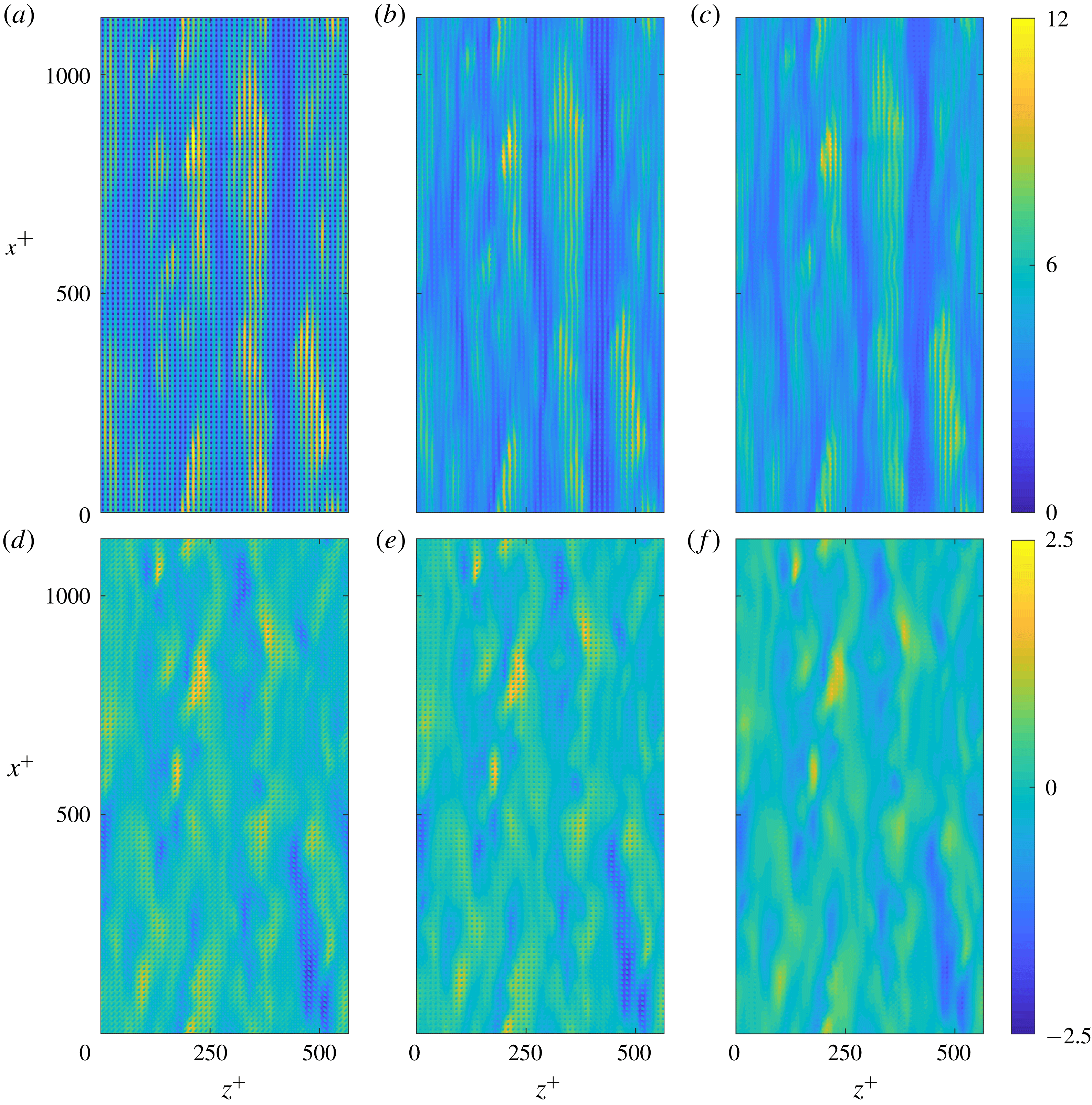
Streamwise (a–c) and spanwise (d–f) instantaneous velocity snapshots for the full velocity field (a,d), the turbulent component obtained from the conventional triple decomposition (b,e) and the turbulent component obtained from the modified triple decomposition (c,f) for the case with $L^{+}\approx 12$ .

Figure 12.

Premultiplied energy spectra at $y^{+}=0$ for the streamwise (a–c) and spanwise (d–f) velocities for the case with $L^{+}\approx 12$ . (a,d) Full velocity fields; (b,e) turbulent components obtained from the conventional triple decomposition; (c,f) turbulent components obtained from the modified triple decomposition.

Figure 13.

One-dimensional premultiplied energy spectra at $y^{+}=0$ of the streamwise (a,b) and spanwise (c,d) velocities for the case with $L^{+}\approx 12$ . $\cdots \cdots$ , full velocity signal; – –, turbulent components obtained from the conventional triple decomposition; ——, turbulent components obtained from the modified triple decomposition.

The result of the above decomposition minimises the signature of the texture in $u_{T}$ and $w_{T}$ . We refer to these as the ‘turbulent’ components in the following discussions. Instantaneous flow fields for the full streamwise and spanwise velocities at the surface for the case with $L^{+}\approx 12$ are shown in figure 11, together with the turbulent velocity fields obtained from both the conventional triple decomposition and the modified decomposition of (3.2)–(3.3). The effectiveness of the two decompositions at isolating the turbulent components of the velocities beyond any particular instant can be better elucidated from two-dimensional premultiplied energy spectra, as shown in figure 12 for the streamwise and spanwise velocities at the surface. The spectra obtained from the full velocity fields show energy at length scales consistent with that observed over smooth walls, as well as coherent energy directly induced by the texture at the wavelengths of the texture and its subharmonics. In addition to this coherent energy, there is texture-induced energy in length scales larger than the texture size that is modulated by the overlying turbulent flow. The relative magnitudes of the energy distribution are clearer after collapsing the data into one-dimensional spectra, as shown in figure 13. The turbulent components of the flow fields obtained from the decomposition should contain no energy at the texture length scales or the modulated texture-induced flow wavelengths. The conventional triple decomposition partially filters out the coherent energy at the wavelengths of the texture, but it has no mechanism to filter out wavelengths larger than the texture size or, for that matter, at wavelengths which are not harmonics of the texture wavelength. Figures 12(a) and 12(d) show that the texture has a dense spectral signature around the texture harmonics, caused by the amplitude modulation with the overlying flow. If the texture-coherent ensemble average is subtracted from the full signal, these surrounding regions remain. In physical space, this can be interpreted as the triple decomposition yielding a too intense coherent flow where the overlying, driving flow is weak, and vice versa. If, on the other hand, the amplitude-modulated texture-coherent flow is subtracted, the surrounding regions are effectively removed. For small textures, there is a clear separation of scales between the spectral region caused by the overlying turbulence and that induced by the texture, and the subtraction of the amplitude-modulated signal is essentially equivalent to filtering out wavelengths below a certain threshold. This is, however, not possible when the different regions overlap (Fairhall & García-Mayoral Reference Fairhall and García-Mayoral2018), while the algebraic solution for $u_{T}$ and $w_{T}$ in (3.2) and (3.3) is still possible.

For the spanwise velocity, the turbulent component contains only a small amount of energy of the texture-induced flow at the texture wavelength. The turbulent component of the streamwise velocity shows energy from modulation of the texture-induced flow in large streamwise wavelengths that has not been filtered. This energy results from the background spanwise velocity inducing streamwise velocity around texture elements, which is not accounted for in (3.2). This effect can be modelled in the decomposition, if the texture size is small, by assuming that the local overlying turbulence acts as a homogeneous transverse shear over texture elements, generating a corresponding coherent flow. This assumption is valid if there is a separation of scales between the texture wavelength and the scales of the overlying turbulence. For small texture sizes, $L^{+}\lesssim 18$ , this assumption is reasonable and including this term for the case shown here, $L^{+}\approx 12$ , filters the energy in large streamwise wavelengths from the background turbulent component. However, for larger texture sizes, $L^{+}\gtrsim 18$ , the texture width becomes larger than that of near-wall vortices (Blackwelder & Eckelmann Reference Blackwelder and Eckelmann1979). Individual texture elements no longer simply perceive an overlying homogeneous shear. In these cases, the inclusion of this term in the decomposition for the streamwise velocity results in spurious noise in the obtained background turbulent fields, $u_{T}$ . For consistency this term is neglected for all cases, but this does not affect the results in the subsequent analysis. The assumption of unidirectional flow over texture elements is also present in the spanwise velocity decomposition. The results in § 3.2 will show that as the texture size is increased this assumption starts to fail, but in these cases the inclusion of this term is still more effective at isolating the background turbulent flow than neglecting it.

Figure 14.

Instantaneous streamwise (a–d) and spanwise (e–h) slip lengths for wavelengths $\unicode[STIX]{x1D706}_{z}^{+}\approx 113{-}565$ and $\unicode[STIX]{x1D706}_{x}^{+}\approx 113{-}1131$ (coloured from red to blue for increasing streamwise wavelength) for the case with $L^{+}\approx 12$ obtained from the full velocity fields. (a,e) Instantaneous correlation of velocity and shear magnitudes; (b,f) probability density histogram of the slip length; (c,g) streamwise and (d,h) spanwise phase difference between velocity and shear. In (a,b,e,f) the dashed line indicates the fitted dynamic slip length, obtained from a linear regression of the data points, and the dotted line indicates the mean slip length.

Figure 15.

Instantaneous streamwise (a–d) and spanwise (e–h) slip lengths for wavelengths $\unicode[STIX]{x1D706}_{z}^{+}\approx 113{-}565$ and $\unicode[STIX]{x1D706}_{x}^{+}\approx 113{-}1131$ (coloured from red to blue for increasing streamwise wavelength) for the case with $L^{+}\approx 47$ obtained from the full velocity fields. (a,e) Instantaneous correlation of velocity and shear magnitudes; (b,f) probability density histogram of the slip length; (c,g) streamwise and (d,h) spanwise phase difference between velocity and shear. In (a,b,e,f) the dashed line indicates the fitted dynamic slip length, obtained from a linear regression of the data points, and the dotted line indicates the mean slip length.

3.2 Homogeneity of the slip length

Once the background turbulent component of the flow has been isolated, we reassess the apparent slip length experienced by the turbulent length scales in the overlying flow. Following Fairhall & García-Mayoral (Reference Fairhall and García-Mayoral2018), we consider the slip length from a spectral perspective, which allows us to discriminate between different length scales in the flow. The slip length in a spectral framework is characterised by both a magnitude and a phase, with the phase having streamwise and spanwise components. The phase of the slip length, $\unicode[STIX]{x1D711}$ , represents the phase lag between the velocity and shear at the surface. For a given wavelength, $\unicode[STIX]{x1D706}$ , the phase is $\unicode[STIX]{x1D711}=2\unicode[STIX]{x03C0}\unicode[STIX]{x0394}/\unicode[STIX]{x1D706}$ , where $\unicode[STIX]{x0394}$ is the spatial offset between the velocity and shear. For a homogeneous slip-length model to be valid, the measured slip length should have a magnitude that is constant in time and across wavelengths, with the velocity and shear in phase. In the following discussion, we refer to two slip lengths, the mean slip length and the dynamic slip length. The mean slip length, $\overline{\ell }_{x}^{+}$ , is the time average of the slip length experienced by the streamwise zero mode, i.e. it is the slip length experienced by the mean velocity profile. The dynamic slip length, $\hat{\ell }^{+}$ , is the time-average slip length experienced by the velocity fluctuations (Seo & Mani Reference Seo and Mani2016). The dynamic slip length is obtained from a linear fit of the instantaneous velocity and shear fluctuations.

It has previously been observed, from analysing the full velocity fields, that the velocity and shear are correlated for small texture sizes (Seo & Mani Reference Seo and Mani2016; Fairhall & García-Mayoral Reference Fairhall and García-Mayoral2018). This correlation can be observed in figure 14, which shows both the slip-length magnitudes and phases for the texture size $L^{+}\approx 12$ . Only a small scatter is present in the observed slip-length magnitude and phase. The wavelengths shown are $\unicode[STIX]{x1D706}_{x}^{+}\approx 113{-}1131$ and $\unicode[STIX]{x1D706}_{z}^{+}\approx 113{-}565$ . These are length scales relevant to the near-wall turbulent dynamics, being of the order of the near-wall vortices and streaks, and are length scales larger than the texture wavelengths. As with previous analysis using the full velocity fields, the value of the dynamic slip lengths, i.e. the slip lengths of the fluctuations, are slightly reduced compared to the mean slip length (Seo & Mani Reference Seo and Mani2016; Fairhall & García-Mayoral Reference Fairhall and García-Mayoral2018).

As the texture size is increased, the correlation between the velocity and shear, and therefore the validity of the slip length model, appears to be lost, as shown by Seo & Mani (Reference Seo and Mani2016) for texture sizes beyond $L^{+}\sim O(10)$ . This is demonstrated in figure 15, which shows the slip lengths obtained from the full velocity fields for the case with $L^{+}\approx 47$ . As discussed in Fairhall & García-Mayoral (Reference Fairhall and García-Mayoral2018) this loss of correlation occurs even for length scales much larger than the texture size, which was attributed to the contamination of the perceived slip length by the texture-induced flow.

Figures 14 and 15 only portray correlations for a subset of wavelengths. To assess the correlation over the full range, figure 16 extends this analysis to time-averaged spectral maps of the dynamic slip lengths. For reference, the spectral energy densities for the corresponding velocities at a height $y^{+}=15$ above the surface are overlaid, to indicate the energetically relevant length scales in the overlying flow. The spectral maps obtained from the full velocity fields show the effects of the contamination of the texture-induced flow. Length scales of the order of the texture size appear to experience significantly reduced slip lengths, while length scales much larger than the texture size appear to experience, on average, a slip length different to the value of the mean slip length. However, the instantaneous correlations in figure 15 showed that for larger texture sizes the concept of a time-averaged slip length loses validity.

Figure 16.

Spectral maps of the slip lengths obtained from the full velocity fields (filled contour) for the streamwise (a,c,e,g,i) and spanwise (b,d,f,h,j) directions, with $L^{+}\approx 12$ –47 shown from top to bottom. Spectral energy density of the corresponding velocity at a height of $y^{+}=15$ (lined contour). The red cross indicates the wavelength of the texture.

Figure 17.

Instantaneous streamwise (a–d) and spanwise (e–h) slip lengths for wavelengths $\unicode[STIX]{x1D706}_{z}^{+}\approx 113{-}565$ and $\unicode[STIX]{x1D706}_{x}^{+}\approx 113{-}1131$ (coloured from red to blue for increasing streamwise wavelength) for the case with $L^{+}\approx 47$ obtained from the turbulent components of the velocity fields. (a,e) Instantaneous correlation of velocity and shear magnitudes; (b,f) probability density histogram of the slip length; (c,g) streamwise and (d,h) spanwise phase difference between velocity and shear. In (a,b,e,f) the dashed line indicates the fitted dynamic slip length, obtained from a linear regression of the data points, and the dotted line indicates the mean slip length.

Figure 18.

Spectral maps of the variation of the slip length, $(\ell _{x/z}-\langle \ell _{x/z}\rangle )/\langle \ell _{x/z}\rangle$ where $\langle \ell _{x/z}\rangle$ is the mean dynamic slip length over the range $\unicode[STIX]{x1D706}_{x}^{+}\approx 113{-}1131$ and $\unicode[STIX]{x1D706}_{z}^{+}\approx 113{-}565$ , obtained from the turbulent components of the velocity fields (filled contour) for the streamwise (a,c,e,g,i) and spanwise (b,d,f,h,j) directions, with $L^{+}\approx 12$ –47 shown from top to bottom. Spectral energy density of the corresponding velocity at a height of $y^{+}=15$ (lined contour). The red cross indicates the wavelength of the texture.

We now reassess the slip-length correlations using the velocity fields of the background turbulent components, $u_{T}$ and $w_{T}$ . These correlations essentially show a collapse to a uniform slip length with zero phase, recovering a good correlation between velocity and shear, as shown in figure 17. It should be noted that use of the conventional triple decomposition to filter the flow fields would yield the same correlations of figure 15. This is because the wavelengths portrayed, $\unicode[STIX]{x1D706}_{x}^{+}$ , $\unicode[STIX]{x1D706}_{z}^{+}>100$ are larger than the texture wavelength, and would therefore be unmodified by the decomposition, as discussed in § 3.1. Recovery of the slip-length correlation for $u_{T}$ and $w_{T}$ can be interpreted as the overlying, background turbulence being subject to a homogeneous boundary condition, i.e. a slip length. This confirms that the loss of correlation of the slip length previously observed is a result of contamination by the texture-induced flow. Further to this, the streamwise dynamic slip length, i.e. the slip length experienced by the velocity fluctuations, recovers the value of the mean slip length, in contrast to the smaller value obtained from the full velocity fields. The previously observed reduction in value, therefore, also appears to be a result of contamination by the texture-induced flow. The spanwise fluctuations, however, still appear to experience a slip length that is smaller than the mean streamwise slip length, despite the isotropy of the texture.

Figure 18 shows spectral maps of the variation of the dynamic slip length for the background turbulent component. These confirm that a homogeneous slip length is recovered across all energetically relevant length scales. The streamwise spectral maps show slip lengths that are homogeneous across all scales, for all texture sizes, with values matching the slip length experienced by the mean flow. All length scales in the flow, therefore, experience the same streamwise slip length as the mean flow. For the spanwise slip length, for all texture sizes, and across all energetically relevant scales, the slip length is also homogeneous. As the texture size is increased, scales of the order of the texture size and smaller show a deviation from the slip length experienced by larger wavelengths. This apparent loss of correlation is likely due to the failure of the decomposition to fully remove the texture-induced flow. As discussed in § 3.1, the decomposition assumes that the flow remains unidirectional over individual texture elements. While for small texture sizes, $L^{+}\lesssim 18$ , this assumption is reasonable, for larger texture sizes, $L^{+}\gtrsim 18$ , the surface texture becomes larger than the near-wall vortices (Blackwelder & Eckelmann Reference Blackwelder and Eckelmann1979), making this assumption questionable. In any event, all relevant length scales in the background turbulent flow perceive the surface as a homogeneous slip length. Consequently, the mismatch between slip-length simulations and texture-resolving simulations, as the texture size is increased, cannot be attributed to the overlying turbulence not perceiving the surface as producing a homogeneous slip effect.

4 The effect of surface slip

In this section we isolate the effect of surface slip on the overlying turbulent flow by replacing the textured surfaces by the corresponding homogeneous boundary conditions, with slip lengths obtained a posteriori from the texture-resolved simulations. The values of the applied slip lengths are given in table 1. From this we will be able to separate the effects of slip and texture on the overlying turbulence.

Equation (1.6) can be interpreted such that the effective spanwise slip length, $\ell _{z,eff}^{+}$ , is the distance below the surface where the overlying turbulence perceives a wall (García-Mayoral et al. Reference García-Mayoral, Gómez-de-Segura and Fairhall2018; Gómez-de-Segura et al. Reference Gómez-de-Segura, Fairhall, MacDonald, Chung and García-Mayoral2018). The flow is therefore described by two virtual origins (Luchini et al. Reference Luchini, Manzo and Pozzi1991), the virtual origin of the mean flow, $\ell _{x}^{+}$ , and the virtual origin perceived by the overlying turbulent flow, $\ell _{T}^{+}$ . Due to the homogeneous slip-length boundary conditions and impermeability of the surfaces considered here $\ell _{T}^{+}\approx \ell _{z,eff}^{+}$ , the empirical relation in (1.5). For the more general case, in which the impermeability condition is relaxed, the turbulent virtual origin deviates from the relation for $\ell _{z,eff}^{+}$ (Gómez-de-Segura et al. Reference Gómez-de-Segura, Fairhall, MacDonald, Chung and García-Mayoral2018).

As the turbulent flow perceives a wall at a distance $\ell _{T}^{+}$ below the surface, we base the scaling for the problem from this virtual origin. The effective half-height of the channel, therefore, becomes the distance from the turbulent virtual origin to the channel centre $\unicode[STIX]{x1D6FF}^{\prime }=\unicode[STIX]{x1D6FF}+\ell _{T}$ , and the friction velocity, $u_{\unicode[STIX]{x1D70F}}$ , is defined at the turbulent virtual origin, $y^{+}=-\ell _{T}^{+}$ .

To compare the result of scaling with this $u_{\unicode[STIX]{x1D70F}}$ and the conventional scaling with the origin at $y^{+}=0$ , the mean velocity profiles, with the slip velocity subtracted, and the r.m.s. fluctuations of the velocities, Reynolds stress and streamwise vorticity are shown in figure 19. The r.m.s. of streamwise vorticity is an indicator of the strength and $y$ -location of quasi-streamwise vortices. The panels (a,c,f,i,l,o) of figure 19 normalise these profiles by the friction velocity obtained at $y^{+}=0$ . Compared to the smooth-wall profiles, these fluctuations show an apparent shift of the location of the peaks closer to the surface, as previously reported (Min & Kim Reference Min and Kim2004; Busse & Sandham Reference Busse and Sandham2012), as well as a slight increase of the magnitudes of the peaks for increasing slip. The panels (b,d,g,j,m,p) of figure 19 show these fluctuations after rescaling by the friction velocity at the turbulent virtual origin, $y^{+}=-\ell _{T}^{+}$ , and shifting the profiles in $y^{+}$ by $\ell _{T}^{+}$ , so that the origin is at $y^{+}=-\ell _{T}^{+}$ . Defined in this way, the profiles show a close collapse to the smooth-wall profiles. This supports the idea that turbulence perceives a virtual origin at $y^{+}=-\ell _{T}^{+}$ , and is otherwise essentially unmodified. There are slight differences to the r.m.s. profiles very close to the surface, most noticeably for the streamwise velocity fluctuations. Figure 19 shows that sufficiently far from the surface the turbulent flow perceives a wall at the turbulent virtual origin $y^{+}=-\ell _{T}^{+}$ . However, as the surface is approached the flow needs to satisfy the imposed boundary conditions, which are the imposed slip lengths. While turbulence perceives an origin at $y^{+}=-\ell _{T}^{+}$ , the streamwise and spanwise velocities would vanish at $y^{+}=-\ell _{x}^{+}$ and $y^{+}=-\ell _{z}^{+}$ , which in our simulations are both deeper into the surface than $y^{+}=-\ell _{T}^{+}$ . This modifies the gradient of the r.m.s. fluctuations very close to the surface. The effect is particularly intense for the streamwise velocity, which has the deepest virtual origin, and even results in a small increase in the value of the peak r.m.s.

Premultiplied energy spectra for the three velocities, Reynolds stress and streamwise vorticity are also shown in figure 19, at a height of 15 wall units above the turbulent virtual origin $\ell _{T}^{+}$ . These spectra also show a collapse to the smooth-wall data. The slip boundary conditions do not alter the turbulent dynamics in the overlying flow, which remains smooth-wall like except for the shift of the origin.

Figure 19.

Velocity fluctuations for the homogeneous slip-length simulations scaled by the friction velocity at the surface (a,c,f,i,l,o), rescaled by the friction velocity based at the turbulent virtual origin and shifted by the turbulent virtual origin, $\ell _{T}^{+}$ (b,d,g,j,m,p): ——, smooth wall; —— (from blue to red), increasing equivalent texture size $L^{+}\approx 12$ to 47. Spectral energy densities at a height $y^{+}+\ell _{T}^{+}=15$ (e,h,k,n,q). Filled contour, smooth wall; —— (from blue to red), increasing equivalent texture size.

5 The effect of surface texture

It has previously been observed that the $\unicode[STIX]{x0394}U^{+}$ obtained from texture-resolving simulations differs from that obtained from homogeneous slip-length simulations when the texture size becomes sufficiently large (Seo & Mani Reference Seo and Mani2016). The ratio of $\unicode[STIX]{x0394}U^{+}$ between the texture-resolving simulations and the equivalent homogeneous slip-length simulations for our cases shows this in figure 20. The results of § 3, however, showed that for texture-resolving simulations the overlying turbulence still experiences a homogeneous slip-length boundary condition, even for textures as large as $L^{+}\simeq 50$ . This indicates that the texture does not modify the boundary condition for the overlying turbulence. The additional downward shift of the mean velocity profile must, therefore, arise from the nonlinear interaction of the texture-induced flow with the overlying turbulence. To investigate the discrepancy in $\unicode[STIX]{x0394}U^{+}$ for larger texture sizes, in this section we compare the results of texture-resolving simulations to homogeneous slip-length simulations. We assume that the effect of slip in the texture-resolved cases is the same as in the homogeneous slip cases and, consequently, the virtual origin of the turbulent flow, $\ell _{T}^{+}$ , is the same as the virtual origin of the corresponding homogeneous slip-length simulation. Any further changes to the flow, compared to the homogeneous slip cases, are then a consequence of the texture.

Figure 20.

Ratio of $\unicode[STIX]{x0394}U^{+}$ measured from the texture-resolved simulations and the equivalent homogeneous slip-length simulations.

Figure 21.

Mean velocity profiles, velocity fluctuations and Reynolds stress for the texture-resolved simulations, scaled by the friction velocity at, and shifted by, the turbulent virtual origin: ——, smooth channel; —— (from blue to red), increasing texture size from $L^{+}\approx 12$ to 47.

Figure 22.

Comparison of fluctuations from the texture-resolved and from the equivalent homogeneous slip-length simulations to smooth channel data, for the cases with (a–c) $L^{+}\approx 18$ ; (d–f) $L^{+}\approx 24$ ; (g–i) $L^{+}\approx 47$ . (a,d,g) Mean velocity profile; (b,e,h) r.m.s. velocity fluctuations (c,f,i) Reynolds stress: ——, smooth channel; –▫–, homogeneous slip-length simulations; –○–, full velocity fluctuations from the texture-resolved simulations; - - - -, turbulent component of velocity fluctuations from the texture-resolved simulations.

Figure 23.

Spectral energy densities of the three velocities and Reynolds stress for the cases with $L^{+}\approx 12$ –47 at a height $y^{+}+\ell _{T}^{+}=15$ . Lines: ——, smooth wall; filled contour, texture-resolved simulations; – –, homogeneous slip-length simulations.

The mean velocity profiles and r.m.s. fluctuations of the velocities and the Reynolds stress for all textured cases are shown in figure 21. The full r.m.s. fluctuations are compared with those from the background turbulence, and with those in homogeneous slip simulations in figure 22, for the cases with $L^{+}=18$ , 24 and 47. For texture sizes $L^{+}\lesssim 20$ the fluctuations and mean velocity profiles from the texture-resolved simulations agree well with the homogeneous slip-length simulations. There is a texture-coherent contribution very close to the surface, but this does not significantly modify $\unicode[STIX]{x0394}U^{+}$ or the fluctuations of the background turbulence. Premultiplied energy spectra are shown in figure 23 at a height 15 wall units above the turbulent virtual origin, $\ell _{T}^{+}$ , where the signature of the texture is already negligible. They show that for $L^{+}\lesssim 20$ the spectra of the texture-resolved simulations essentially collapse to the spectra from simulations over smooth walls. For textures of this size, the predominant effect of the surface is the effect of surface slip. The shift $\unicode[STIX]{x0394}U^{+}$ for these texture sizes can be predicted by the homogeneous slip-length simulations.

Figure 24.

Streamwise (a,d), wall-normal (b,e) and spanwise (c,f) instantaneous velocity fluctuation flow fields, at a height $y^{+}+\ell _{T}^{+}=15$ , for a smooth wall (a–c) and the turbulent component of the velocities for the case with $L^{+}\approx 47$ (d–f).

Beyond $L^{+}\gtrsim 25$ , however, there are further modifications to the r.m.s. fluctuations than the sole effect of slip. Near the surface, the texture-induced coherent fluctuations become stronger, as previously reported (Jelly et al. Reference Jelly, Jung and Zaki2014; Türk et al. Reference Türk, Daschiel, Stroh, Hasegawa and Frohnapfel2014; Seo et al. Reference Seo, García-Mayoral and Mani2015). Additionally, with increasing texture size, the Reynolds stress profiles show a modified shape compared to smooth-wall turbulence with an increase in Reynolds stress for $y^{+}\lesssim 25$ . The contribution of the texture-coherent component to the Reynolds stress is negligible, so the observed difference is essentially caused by modifications in the background turbulence. This additional Reynolds stress results in a further downward shift of the mean velocity profile, and the corresponding reduction in $\unicode[STIX]{x0394}U^{+}$ . The near-wall peak of the streamwise fluctuations is also reduced compared to the peak observed over smooth walls. The wall-normal and spanwise fluctuations show an increase beyond the additional texture-induced fluctuations. This persists up to $y^{+}\sim 50$ and has previously been reported in flows over superhydrophobic surfaces (Seo et al. Reference Seo, García-Mayoral and Mani2015). It is a phenomenon also observed over rough surfaces (Antonia & Krogstad Reference Antonia and Krogstad2001; Orlandi & Leonardi Reference Orlandi and Leonardi2006). The premultiplied energy spectra show that beyond $L^{+}\gtrsim 25$ there is an increase of energy in shorter streamwise length scales, and a decrease of energy in longer streamwise length scales, compared to smooth-wall turbulence. The wall-normal velocity also shows an increase of energy in larger spanwise wavelengths. These are also a phenomenon seen over surfaces with roughness (Krogstad & Antonia Reference Krogstad and Antonia1994; Abderrahaman-Elena et al. Reference Abderrahaman-Elena, Fairhall and García-Mayoral2019). Instantaneous realisations of the fluctuating velocity components over a smooth wall and of the background turbulent component of the case with $L^{+}\approx 47$ are shown in figure 24 at a height $y^{+}+\ell _{T}^{+}=15$ . The latter show a reduction in streamwise coherence for scales of order 1000 wall units, as is also indicated by the energy spectra. At such large texture size, the length scales and magnitude of the texture-coherent flow become comparable to those of the background turbulence. The spectra and instantaneous flow fields suggest a modification of the near-wall dynamics through the disruption of streaks and quasi-streamwise vortices by the texture-induced flow.

These results show that, while the overlying turbulent flow still experiences the surface as imposing a homogeneous slip-length boundary condition, for sufficiently large textures, a nonlinear interaction of the texture-induced flow with the overlying turbulence modifies its dynamics. This interaction has an extended $y$ -support and does not occur only at $y^{+}=0$ . For the texture layout considered in this work, this nonlinear interaction begins to appear for $L^{+}\simeq 25$ and becomes significant for $L^{+}\gtrsim 30$ . This is therefore the upper limit where homogeneous slip lengths are valid, at least for the geometry studied here. Note that $L^{+}\gtrsim 30$ was also the limit established by Seo et al. (Reference Seo, García-Mayoral and Mani2018), beyond which the air–water interface can be expected to become unstable, so that drag reduction predictions would cease being meaningful. Different texture layouts could, however, cause different texture-induced flows, modifying the onset of the nonlinear interaction.