




1. Introduction
Intermediate-mass black holes (IMBHs) are black holes (BHs) between 100 and
 $10^4 M_{\odot}$
. BHs less massive than
 $\sim 100 M_{\odot}$
are well known as stellar-mass BHs. Before the detection of gravitational waves (GWs) (Abbott et al. Reference Abbott2016), they were found as X-ray binaries (Corral-Santana et al. Reference Corral-Santana2016). On the other hand, BHs more massive than
 $\sim 10^5 M_{\odot}$
are also known as supermassive BHs (SMBHs). SMBHs are located at the center of galaxies (Kormendy et al. 2013), and one exists at the center of the Milky Way galaxy (GRAVITY Collaboration 2019). Most of them are known as active galactic nuclei (AGNs) (Mezcua Reference Mezcua2017), and the BH masses are estimated from their luminosity (Reines, Greene, & Geha Reference Reines, Greene and Geha2013):
 \begin{equation}\log \left(\frac{M_{\rm{BH}}}{M_{\odot}}\right)=\log \epsilon+6.57 +0.47 \log \left(\frac{L_{\rm{H}_\alpha}}{10^{42} \rm{erg} \rm{~s}^{-1}}\right) +2.06 \log \left(\frac{\rm{FWHM}_{\rm{H} \alpha}}{10^3 \rm{~km} \rm{~s}^{-1}}\right),\end{equation}
where
 $M_{\rm BH}$
,
 $L_{\rm H\alpha}$
, and
 $\rm{FWHM}_{\rm H\alpha}$
are the black hole mass, H
 $_{\alpha}$
luminosity, and full width at half maximum of the
 $H_{\alpha}$
line. The least luminous AGNs are estimated to have SMBHs of several
 $10^4 M_{\odot}$
, which is the massive end of IMBHs.
Stellar-mass BHs have been found as X-ray binaries (Corral-Santana et al. Reference Corral-Santana2016). The most luminous one, Hyper-Luminous X-ray Source 1 (HLX-1) is estimated to have a
 $\sim 500$
–
 $20,000 M_{\odot}$
BH (Farrell et al. Reference Farrell, Webb, Barret, Godet and Rodrigues2009) (Godet et al. Reference Godet, Plazolles and Kawaguchi2012). HLX-1 is located in a globular cluster in the galaxy ESO 243–49.
GW has also suggested the existence of BHs over
 $100 M_{\odot}$
such GW190521, which is
 $140 M_{\odot}$
formed from
 $85+66M_{\odot}$
(Abbott et al. Reference Abbott2020), and GW231123, which is
 $225M_{\odot}$
formed from
 $137+103 M_{\odot}$
(The LIGO Scientific Collaboration et al. 2025). These correspond to the low-mass end of IMBHs.
IMBHs with a few thousand to
 $10^4 M_{\odot}$
are in a range that is hardly observable. Another way to detect IMBHs is through the kinematics of globular clusters. The central region of globular clusters is one possible site of IMBHs. If we could measure the steep rise of the velocity dispersion, it would be a sign of IMBHs (Lützgendorf et al. Reference Lützgendorf2013).
Some numerical simulations of star clusters have suggested the formation of IMBH via runaway collisions of stars in young star clusters (Portegies Zwart et al. Reference Portegies Zwart, Baumgardt, Hut, Makino and McMillan2004), and these simulations started from initially spherical and dynamically in equilibrium state. However, star-forming regions are not spherical or in equilibrium. Therefore, star clusters may also have formed similarly in turbulent molecular clouds. In such a case, the highest density of star clusters may have been achieved during their formation phase, when star clusters were still embedded in their parental molecular clouds. We, therefore, performed star cluster formation simulations starting from turbulent molecular clouds, integrating stars as collisional systems.
2. ASURA+BRIDGE
For the simulations, we used an N-body/smoothed-particle hydrodynamics (SPH) code, ASURA+BRIDGE code (Hirai et al. Reference Hirai, Fujii and Saitoh2021), which can treat stars as a collisional system. ASURA+BRIDGE code is based on an N-body/SPH code, ASURA (Saitoh et al. Reference Saitoh, Daisaka and Kokubo2009), but the N-body integration is calculated using PeTar code (Wang et al. Reference Wang, Iwasawa, Nitadori and Makino2020). They are combined using the BRIDGE scheme (Fujii et al. Reference Fujii, Iwasawa, Funato and Makino2007). Here, we summarize the ASURA+BRIDGE code in the following.
-
• ASURA: ASURA is an N-body/SPH code adopting density independent SPH scheme (Saitoh & Makino Reference Saitoh and Makino2013). It also adopts the FAST scheme (Saitoh & Makino Reference Saitoh and Makino2010), in which gas particles are integrated with timesteps smaller than those for self-gravity.
-
• Particle-particle particle-tree (P
 $^3$
T) scheme: a hybrid integrator of fourth-order Hermite scheme and leapfrog integrator with tree scheme initially developed for proto planetary disks (Oshino et al. Reference Oshino, Funato and Makino2011) and later applied for globular clusters (Iwasawa et al. Reference Iwasawa, Portegies Zwart and Makino2015). In P
$^3$
T scheme, the interaction within a given radius (short-range force) is integrated using the Hermite scheme with individual timesteps, but the other interaction (long-range force) is calculated using the tree scheme (Barnes & Hut Reference Barnes and Hut1986) and integrated using the leapfrog integrator with a shared timestep. P
$^3$
T scheme enables the integration of a million particles as a collisional system.
-
• PeTar: a P
$^{3}$
T scheme code with a slow-down algorithmic regularization (SDAR) scheme for binaries (Wang et al. Reference Wang, Iwasawa, Nitadori and Makino2020). The SDAR scheme enables the integration of hard binaries without gravitational softening. -
• BRIDGE: a hybrid integration scheme similar to P
$^3$
T. BRIDGE was initially developed for star clusters in a galaxy, in which star clusters were integrated with a high-order integrator as collisional systems, and the galaxy was integrated using a leapfrog integrator with a tree code. In ASURA+BRIDGE, stars are integrated using PeTar as a collisional system, but gas is integrated using tree code and leapfrog integrator, and they are combined in every BRIDGE timestep. -
• Probabilistic star formation: This scheme is often used for galaxy simulations. Once a gas particle satisfies the criteria for star formation, it forms a star particle. We adopted the following as the criteria; (1) density threshold (
$n_{\rm{th}}\gt10^5$
cm
$^{-3}$
), (2) temperature threshold (
$T_{\rm{th}} \lt 30$
K), and (3) the divergence of the velocity is less than zero. We assumed a star formation efficiency as 2 % of the local free-fall time (Krumholz, Dekel, & McKee Reference Krumholz, Dekel and McKee2012). See also (Hirai et al. Reference Hirai, Fujii and Saitoh2021) for more details. The mass of the forming star is drawn from a given IMF. We adopted Kroupa IMF (Kroupa & Weidner 2023). If the drawn mass is larger than half of the gas mass within a given search radius (
$0.2$
pc), we draw the stellar mass again. The star particle was formed by taking mass from gas particles within the search radius. -
• HII region model: Instead of solving radiation hydrodynamics, we calculated Strömgren radius using the local gas density around the massive star and increased the gas temperature in the radius to
$10^4$
K. We also added mechanical feedback due to the stellar wind to the gas particles within the radius as radial velocities (Renaud et al. Reference Renaud2013). If the calculated Strömgren radius is smaller than the distance to the nearest gas particle, we added the mechanical feedback to the gas particles within the gravitational softening length for gas particles. We used the OSTAR model (Lanz & Hubeny Reference Lanz and Hubeny2003), which is a table based on the numerical modeling of massive stars, for the photon counts. Since the photon counts drop around 8–10
$M_{\odot}$
, we adopted this feedback only from stars more massive than
$8 M_{\odot}$
. See (Fujii et al. Reference Fujii, Saitoh, Wang and Hirai2021) for more details. -
• Stellar evolution: stellar evolution using the Single Stellar Evolution (SSE) code (Hurley, Tout, & Pols Reference Hurley, Tout and Pols2002) (Banerjee et al. Reference Banerjee2020). We modified this from SSE’s constant value (
$\dot{M}=1.5\times10^{-4}M_{\odot}$
yr
$^{-1}$
) to the mass loss rate given by (Vink Reference Vink2018): (2)
\begin{equation} \log[\dot{m}_{\rm SW}/M_{\odot}\,{\rm yr}^{-1}] = -9.13+2.1\log[m/M_{\odot}] + 0.74\log[Z/Z_{\odot}]. \end{equation}
-
• Chemical evolution: The abundance of each gas and stars are treated using a chemical evolution library, CELib (Saitoh Reference Saitoh2017). The lost mass from massive stars were added to gas particles within the Strömgren radius, and the new abundance was calculated. CELib also treats the mixing of the elements among gas particles.
-
• Stellar collision: We assumed a sticky sphere approximation for the stellar collision and merger. When two stars approach closer than the sum of their radii, these stars merge without mass loss. When they merge, we assumed that the age of the primary-mass star is the stellar age of the merger remnant. For SSE, we also need to assume the initial mass of the merger remnant. We assumed the sum of the initial mass of the primary-mass star and the current mass of the secondary-mass (lower-mass) star as the initial mass of the merger remnant.
-
• Very massive star: For stars with
$\gt1000M_{\odot}$
, we extrapolated the stellar evolution model in SSE. However, we used the radius and luminosity of the zero-age main sequence, because the values of later times are sometimes unstable.


3. Initial conditions
We adopted a turbulent molecular cloud for our initial conditions (Bonnell et al. Reference Bonnell, Bate and Vine2003). We set up an initially homogeneous spherical molecular cloud with masses of either
 $10^5$
or
 $10^6M_{\odot}$
and metallicity of
 $0.02Z_{\odot}$
and
 $0.1Z_{\odot}$
, similar to observed globular clusters (Harris Reference Harris1996). We adopted radii of 5 and 10 pc for those two masses, respectively, to produce a similar initial density. As a result, in all cases, their initial free-fall time is 0.5–0.6 Myr.
The initial turbulent velocity field is assumed to be a divergence-free Gaussian random field with a power spectrum P(k), varying as
 $k^{-4}$
, where k represents the wave number (Bonnell et al. Reference Bonnell, Bate and Vine2003). We set the initial virial ratio (
 $\alpha_{\rm vir}=|E_{\rm k}|/|E_{\rm p}|$
, where
 $E_{\rm k}$
and
 $E_{\rm p}$
are the total kinetic and potential energies, respectively), to be 0.1. We set the initial gas-particle mass to be
 $0.1 M_{\odot}$
. The initial temperature was set to be 30 K (Fujii et al. Reference Fujii, Wang and Tanikawa2024).
4. Results
The star formation proceeded in the initial free-fall time of the gas (
 $\sim 0.5$
Myr). Stellar collisions occurred especially in the most massive clump of the simulation, in which the central density of the cluster exceeded
 $10^7M_{\odot}$
pc
 $^{-3}$
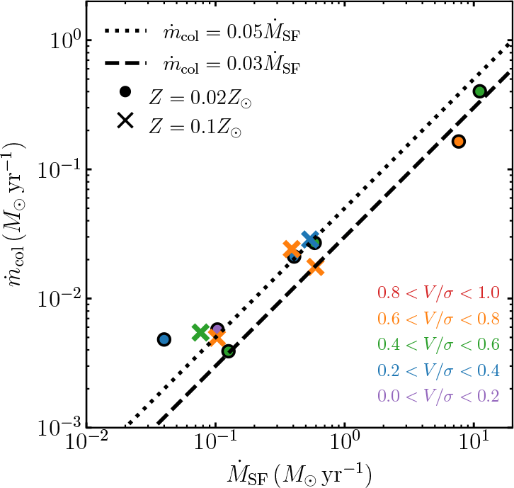
. In Figure 1, we present the relation between the mass increase rate of the cluster due to the star formation and the mass increase rate of the most massive star due to the stellar collisions. We found that 3–5 % of the stellar mass formed in star clusters was provided to the VMS. Our most massive star cluster evolved to
 $5\times 10^5M_{\odot}$
, and a VMS with
 $10^4M_{\odot}$
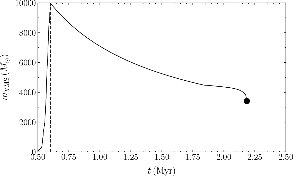
formed in it. We show the mass evolution of this VMS due to runaway collision in Figure 2.
Relation between the mass increase rates of the most massive star and cluster. Colors indicate the rotation of clusters.

Figure 1 Long description
Panel A: A scatter plot depicting the relationship between the mass increase rates of the most massive star and cluster. The horizontal axis represents the mass increase rate of the star-forming region in solar masses per year, ranging from 0.01 to 10. The vertical axis represents the mass increase rate of the collapsing region in solar masses per year, ranging from 0.001 to 10. Data points are marked with circles and crosses, indicating different metallicities. Two dashed lines represent different rates of mass increase. Colors indicate the rotation of clusters.
Mass evolution of the VMS through runaway collisions (before 0.6 Myr) and due to stellar evolution (after 0.6 Myr). The black dot indicates the time and mass when a BH was formed. Vertical dashed line indicates 0.6 Myr, at which we stopped our simulation.

We also analyzed the rotation in a way similar to that adopted in observations, the mean line-of-sight velocity normalized by the velocity dispersion. Our simulations have the six-dimensional data (positions and velocities) of each star. We, therefore, identified the rotation axis by calculating the inertia tensor and then determining the mean line-of-sight velocity (V) along with the rotation axis. We adopted this as the rotation velocity. We also measured the line-of-sight velocity dispersion at each radius (
 $\sigma(r)$
). We found that the rotation velocity normalized by the velocity dispersion (
 $V(r)/\sigma (r)$
) peaks at around 0.03 pc. We, therefore, defined
 $V(r\lt0.02{\rm pc})/\sigma (\lt0.02{\rm pc})$
as the rotation of the cluster. This value is almost equivalent to the peak velocity normalized by the line-of-sight velocity dispersion. As shown in Fig. 1, we did not find any relation between the cluster rotation and collision rate.
After the formation of a very massive star via collisions, the feedback due to the Hii region blew away the gas from the cluster and terminated the star formation. We stopped the simulation there, and the following stellar evolution using SSE (the version we have in PeTar code). In our case, this star loses
 $\sim 6000 M_{\odot}$
and finally leaves a
 $3400 M_{\odot}$
IMBH. This evolution is shown in Figure 2.
5. Summary
We developed a novel N-body/SPH code, ASURA+BRIDGE, and performed star cluster formation simulations from turbulent molecular clouds. We combined an N-body simulation code, PeTar, with an SPH code, ASURA. With PeTar, we can integrate stars, including hard binaries, without gravitational softening. With this code, we can treat star clusters as collisional systems, including stellar collisions.
The most massive clouds formed a star cluster as massive as globular clusters. In this cluster, a runaway collision of stars occurred, and a very massive star with
 $\sim 10^4 M_{\odot}$
formed. Typically, 3–5 % of star cluster mass went to the VMS. According to the stellar evolution model (SSE), it evolves to a
 $3400 M_{\odot}$
IMBH.

 Open access

