Forecasting provides the opportunity to put one's self to the test. Are our models of voting behavior accurate? It is easy to retrofit an explanation for what has happened in the past. Taking a chance on a forecast that can go wrong does not afford us that luxury. Forecasting can also teach a lesson in humility. Over the last decade, political scientists have been willing to gamble on their models. We have had some success. Everyone on the forecasting panel at the 1996 APSA Annual Meeting correctly forecast a Clinton victory. The forecasting of the 2000 presidential election was clearly a lesson in humility (at least for this author). None of the authors of this symposium forecast a Bush victory. Moreover, many forecast a rather substantial victory for Al Gore.1
Technically, we did get it right. After all, we were forecasting the popular vote, which Al Gore did win.
Despite the problems inherent in forecasting, it still has considerable value.2
See Campbell and Garand (2000) for a discussion of the utility of political forecasting.
Assuming we move beyond the simplistic World Series, longest name, and tallest candidate rules, we can actually test our theories of voting behavior. Forecasting also implies that the further before an event we offer the forecast, the more its potential value. A forecast a day or two before the election probably does not offer us much insight beyond what we can get from the news the night before the election. The earlier the forecast the greater the value. Compare a weather forecaster who offers the forecast of a tornado that will hit in five minutes versus a forecaster who offers the forecast a few hours, or days, in advance. Which one has done a better job? Which one has provided a more useful service?
Influences on Election Outcomes
Several factors are quite reasonably thought to be related to presidential election outcomes. Many of the forecasting models take the state of the economy into account. Virtually all of these take some measure of how the economy has performed in the past (Abramowitz 2000; Campbell 2000; Fair 1988; Holbrook 2000; Lewis-Beck and Tien 2000; Lewis-Beck and Wrighton 1994; Lockerbie 2000; Norpoth 2000; Wlezien and Erikson 2000). Several in the forecasting industry have also begun to take into account that voters' economic expectations (Lewis-Beck and Tien 2000; Lockerbie 2000; Norpoth 2000; Wlezien and Erikson 2000). While both likely play a role in why people vote the way they do and why elections turn out like they do, my own work, both in forecasting and individual level vote choice models (Lockerbie 1992; 2000), shows that prospective evaluations are stronger. In the interest of parsimony (given that I have so few cases), it makes sense to trim the number of variables in the model. Consequently, I make use of a prospective item from the Index of Consumer Sentiment in the Survey of Consumer Attitudes and Behavior that concerns what people think will happen to their personal finances over the next year (denoted Next Year Worse).3
Thanks to John Prechtel at the University of Georgia for obtaining the latest data from Rebecca McBee Bono at the Survey of Consumers at the University of Michigan. The earlier data is available at the web site <http://www.sca.isr.umich.edu/>
To make the forecast well in advance of the actual event, I make use of the responses from the first quarter of the election year. Specifically, the question asks “Now looking ahead—do you think that a year from now you (and your family living here) will be better off financially, or worse off, or about the same as now?” The percentage stating the next year will be worse is the score for this variable. This item clearly focuses on the individual and on the future. There is one problem with this item; it makes no statement of attribution of responsibility. The respondents could think their finances are going to improve through the dint of their own efforts or decline due to other events, such as because their boss was just found out to have improperly made use of company assets. Kramer (
1983) and Lockerbie (
1992;
2002) argue that for the economy to influence political attitudes and behaviors, there should be some sense of attribution to political actors. We can take some comfort in that the problem with the item used here is that it biases us against finding a relationship.
Aside from the economy, we should also take into account the potential for an incumbency advantage or penalty. Some might argue that when a president seeks reelection, he might have an advantage. Voters might be willing to give the individual the chance to fully implement his program. One term might not be enough. A third term for a party is another thing. After eight years, voters might experience party fatigue. Also, it will not be the leader of the party seeking a third term, àla Franklin Roosevelt. Instead, it will be (or at least in recent history it has been) the incumbent vice president. At this point voters might be looking for a change, or at least sympathetic to the arguments of the opposition party. Similarly, even if the incumbent vice president is victorious, voters might not be inclined to give one party 16 years of uninterrupted power. Consequently, the model employs a variable (denoted Term Two and Beyond) to account for this possibility. This is scored 0 if the incumbent president, or his party, is seeking his first reelection. It is scored 1 in all other years.
Presidential Election Outcomes
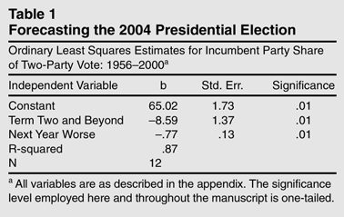
How well does this model forecast when confronted with the data? The equation in Table 1 shows the results of regressing the two-party vote share of the incumbent party on the two independent variables.4
Given the small size of the data set and the potential for an outlying case to make a difference, I reran the analysis using least median squares regression. The results are largely the same. Consequently, the results are not likely to be the result of making use of one particular statistical technique.
With an R-squared of .87, the equation fits the data reasonably well. Both independent variables are statistically significant and in the expected direction. First, the more pessimistic the nation is about personal finances, the worse the incumbent party does when seeking reelection. The incumbent party loses approximately three-quarters of a percentage point of the two-party popular vote for every one percentage point increase in people who are pessimistic. The range on this item is from a low of 6 in 1956, 1964, and 2000. The high on this variable is 25.33 in 1980.
5 The mean is 9.79 and the standard deviation is 5.22.
Moving from the minimum to the maximum translates to a more than 14-point swing in vote share. Second, the party that hopes for reelection after winning two consecutive elections has a rough road to hoe. The coefficient on this item indicates that when a party seeks to move beyond two terms, it loses on average almost nine percentage points. Given the relative closeness of American presidential elections, this is not an inconsequential sum.
Out-of-Sample Forecasts
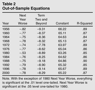
How good a job does the equation do? Are the results driven by one aberrant year? Instead of using the entire data set and the equation for the entire data set to assess the verisimilitude of the model, I make use of out-of-sample forecasts. I simply reestimate the equation with the year I wish to forecast (or, since it as after the fact, ex post forecast) excluded. In other words, I remove one year from the data set, reestimate the equation, and then evaluate the equation. I then take the actual values for the independent variables for the excluded year and plug them into the equation to generate the forecast for that year. This procedure allows two things. First, we can assess the stability of the model by looking at the coefficients for the variables with a single year excluded at a time. Do the coefficients change dramatically? Does the statistical significance of the variables change with a single year excluded? Second, how good a job does the model do in forecasting the excluded year.
Table 2 shows the equations used to generate the out-ofsample forecasts. The first thing to note is the stability of the coefficients. With the exception of the equation with 1980 excluded, the coefficients for the economic variable are within one-half a standard error. In fact, with the exception of the equations excluding 1956 and 1980, the coefficients are within one-seventh of a standard error. For the equation excluding 1980, the coefficient is within two standard errors. We should note that this is the year that the economic item hovers at the edge of statistical significance. Nonetheless, it does hover on the good side of the line. Turning to the time in the White House variable, the coefficients are within one standard error in every instance. Regardless of the year excluded, the R-squared never falls below .84. Looking at the R-squareds also shows us a great deal of similarity; the range on the R-squareds is only .06.
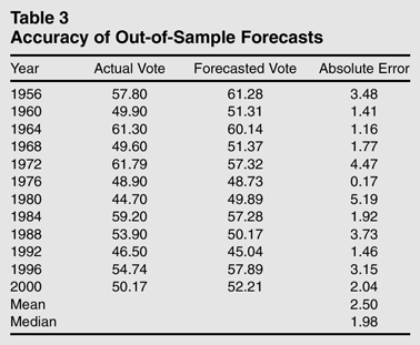
We should also look at the point estimates to ascertain how good a job the equation forecasts. With the out-of-sample equations, we can test their forecasting ability without using the data points we are forecasting to generate the forecast we are examining. The model performs reasonably well. Given the timing of the forecast, the typical forecasting error is remarkably small (mean=2.50, median=1.98). There are two elections that are misforecast: 1960 and 1968. Even here, the forecast errors are not terribly large. In 1960, the error is less than one and one-half percentage points. In 1968, the error is less than two percentage points.
Forecast 2004
How does 2004 look? Plugging the values for the independent variables (Next Year Worse=9.67 and Term Two and Beyond=0) into the equation yields a forecast of 57.6% of the two party vote for President Bush.
How certain should we be of the forecast for 2004? There are several ways in which one can look at this. First, note that for the equation to mis-forecast the victor, it would have to be off by more than seven percentage points. Given that the largest error from the 12 out-of-sample forecasts so far is just over five percentage points, we can, following Campbell (2000, 29), argue that we have a less than one in 12 chance of being wrong in the prediction of a Bush victory. We can also make use of the confidence interval around the prediction, as suggested by Beck (2000, 164). Since the forecast shows Bush winning with 57.6% of the two-party vote and the standard error of the forecast is 2.51, the t value of 3.03 tells us that the confidence is somewhat better than 99%, onetailed. In short, two of the standard tests of certainty lead one to believe with a high degree of confidence that Bush will win reelection.
Conclusion
This forecast speaks to our models of voting behavior. Many of the economic models of voting behavior argue that voters look to the future when casting ballots. While we cannot make direct statements about individuals from aggregates, the findings here are wholly consistent with the hypothesis that voters are looking to the future when casting ballots. Voters might be asking “What will you do for me?”
What does all of the preceding tell us? Elections appear to be predictable events. By taking a few bits of information that are available well before the campaign, we can forecast the outcome of elections quite well. These items are set well before the campaign begins in earnest. We can measure the time a party has controlled the White House as the previous election is called in the media. The item that comes from the election year itself is the measure of voters' expectations concerning their personal financial well-being, and this is available before the parties' conventions. In short, we can make quite accurate forecasts before the parties have officially nominated their standard bearers.