

1 Introduction
In his recent bid for the presidency of the Association for Mathematics of Language, Makoto Kanazawa writes:Footnote *
The scientific study of language is such a large and important field that it's strange that so little mathematical research is being carried out. By comparison, the latest issue of Journal of Economic Theory has 14 original articles, and all but one of them are mathematical papers in the sense of containing theorems and proofs. And the title of the journal is not ‘Journal of Mathematical Economics’, which is actually a separate journal.Footnote 1
That linguistics lags behind economics is not surprising: making more money is a stronger drive for change and progress than better understanding the language faculty. But Bruce Tesar's book shows that the time might be ripe for change and progress in our field as well. Employing a formally sophisticated analytical approach (as opposed to a purely simulation-based approach), the book provides a beautiful example of the interplay between learnability and structural assumptions on the typological space. It thus shows that computational phonology has become a mature subfield of generative linguistics.
Tesar's book formalises the notion of output-drivenness, and explores its phonological meaning, its OT characterisation and its implications for learnability. Informally, a phonological grammar is output-driven provided ‘disparities between input and output are only introduced to the extent necessary to satisfy output restrictions’ (p. 1). Chapter 2 formalises this intuition into a notion of output-drivenness defined independently of the phonological formalism assumed (e.g. SPE, OT, HG). The phonological underpinning of this notion is illustrated by showing that non-output-drivenness unifies a number of phonological phenomena such as chain shifts, derived environment effects and opacity. Chapter 3 focuses on OT and provides a sharp characterisation of output-drivenness in OT grammars. It shows that output-drivenness in OT depends on the nature of the faithfulness constraints, and provides a characterisation of the faithfulness constraints which guarantee output-drivenness. Chapter 4 then surveys and systematises a number of OT approaches to non-output-driven phonological phenomena using the formal characterisation obtained in Chapter 3. Chapters 7 and 8 explore the implications of output-drivenness for OT learnability, focusing on the problem of simultaneously learning a grammar and a lexicon of underlying forms from paradigmatic information. Chapter 1 provides an informal overview, Chapters 5 and 6 review selected prior work on OT learnability and Chapter 9 wraps up.
The book is a difficult read. In this review article I attempt to offer a reader's guide, focusing on the learnability implications of output-drivenness (which are perhaps less accessible to the readership of this journal than its phonological implications). I thus start right away in §2 with a review of the learning problem tackled by Tesar, and pause to discuss two notions of efficient learning, a looser and a more demanding one. In §3, I review Tesar's notion of output-drivenness, tailored to the rather restrictive representational framework considered in his statement of the learning problem. In the rest of the review, I tackle the following question: what can output-drivenness do for the learner? I address this question from two perspectives. In §4, I focus on time complexity: does output-drivenness help the learner to tackle the learning problem faster? In §5, I focus on correctness: does output-drivenness help the learner to better succeed in solving the learning problem? In order to address these questions, I compare Tesar's Output-driven Learner (ODL) with Merchant's (Reference Merchant2008) state-of-the-art Contrast Pair and Ranking Information (CPR) learner, which is only briefly described in Tesar's book. For completeness, CPR is reviewed in Appendix A of the supplementary online materials.Footnote 2
CPR and ODL share the same architecture, in that both maintain partial lexical and grammatical (ranking) information, which are incremented iteratively by boosting one type of partial information against the other. Furthermore, the subroutines used by ODL are a speeded-up version of those used by CPR, as explained in Appendix B. §4 quantifies the speed-up afforded by output-drivenness by comparing the efficiency of CPR's and ODL's subroutines, using both the generous and demanding notions of efficiency introduced in §2. CPR and ODL use two types of subroutines: one for the extraction of ranking information and the other for the extraction of lexical information. Furthermore, these subroutines can be applied to two types of data: either to a single entry in the paradigm or to a pair of entries which share a morpheme (a contrast pair), and are thus able to display morphophonemic alternations. Output-drivenness affords a huge speed-up of the subroutine which extracts ranking information from a single paradigmatic entry: while Merchant's original subroutine is optimal, but (plausibly) inefficient even relative to the looser notion of efficiency, Tesar's restatement under the assumption of output-drivenness is efficient even relative to the more demanding notion. Furthermore, output-drivenness affords a substantial speed-up of Merchant's subroutine for the extraction of lexical information from a single paradigmatic entry: while the original subroutine is only efficient relative to the looser notion of efficiency, Tesar's restatement under the assumption of output-drivenness is efficient even relative to the more demanding notion. Unfortunately, output-drivenness is not helpful when these subroutines are applied to contrast pairs: Merchant's subroutine for the extraction of ranking information from contrast pairs remains inefficient, and the subroutine for the extraction of lexical information from contrast pairs remains efficient only relative to the looser notion of efficiency.
§5 turns from time complexity to correctness. It is easy to formally characterise a class of cases where Merchant's CPR is provably bound to fail. The trouble stems from the fact that CPR is excessively prudent: whenever a paradigm is consistent with a feature being set underlyingly to two different values, CPR refuses to make a choice. If that happens for two features whose values are correlated, CPR inevitably falls short of success. This is, as far as I can tell, the core weakness of CPR's approach. And output-drivenness does not help. Indeed, since Tesar's ODL uses subroutines which are (faster but) equivalent to CPR's subroutines, it inherits CPR's excessive prudence. The crucial question of whether any such problematic case is actually attested in natural language phonology is left open at this stage. Yet this interplay between the typology of what is attested and the formal restrictions on what is learnable demonstrates how relevant this line of research is for phonological theory.
2 The problem of learning languages from paradigms
This section introduces the learning problem tackled in Tesar's book, namely the problem of learning a language from a paradigm within an assigned typology of languages. §2.1 defines the typological space, §2.2 and §2.3 introduce the notions of language and paradigm and §2.4 puts the pieces together, in an explicit statement of the learning problem. §2.5 simplifies the learning problem through some additional rather restrictive representational assumptions, and §2.6 discusses two notions (one more generous, the other more demanding) of the time complexity of a learner.
2.1 Typology
Let ℛ and  be finite sets of
underlying
roots and underlying
suffixes
respectively. They are assumed to be disjoint, so that it is always possible to
tell whether a given underlying morpheme is a root or a suffix. A generic
underlying root is denoted by a bold capital letter from the beginning of the
alphabet (A, B, …), and a generic
underlying suffix by a bold lower-case letter (a, b,
…). As illustration, assume that the underlying roots consist of the
consonant /p/ plus a vowel which is either short or long and either stressed or
unstressed, as (1a), and that the
underlying suffixes have a different consonant, /k/, as in (1b).
-
(1)


Let 핉 and 핊 be the sets of meanings for underlying roots and suffixes respectively. For convenience, they are assumed to be disjoint and to contain exactly one meaning for each underlying root and suffix. A generic root meaning is denoted by M and a generic suffix meaning by m. An example is provided in (2).
-
(2)

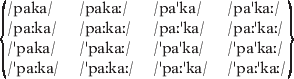
The set of underlying forms consists of all concatenations of a root and
a suffix. A generic underlying form is thus denoted by Aa,
Bb, … . Since the sets
ℛ and of underlying roots and
suffixes are disjoint, the root and the suffix in any given underlying
concatenation can always be pulled apart. In our example, the set of underlying
forms thus consists of the 16 concatenations of the four underlying roots with
the four underlying suffixes, as in (3).
-
(3)
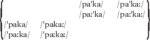
A generating function Gen maps an underlying concatenation Aa of an underlying root A and an underlying suffix a to a set of candidate surface forms. We assume that the set of surface forms is some subset of the set of root/suffix concatenations. Thus again, the root and the suffix in any given surface concatenation can always be pulled apart. A concatenation is denoted with letters from the end of the alphabet when it is construed as a surface form: e.g. Xx, Yy, Zz. Furthermore, we assume that all underlying forms share the same candidate set. In our example, we could thus define the candidate set shared by all underlying concatenations as the subset (4) of the eight root/suffix concatenations which have exactly one stress.
-
(4)
Finally,  is a finite set of
phonological constraints. Each constraint takes an underlying
concatenation Aa and a surface candidate concatenation
Xx and returns the corresponding number of violations. Consider the
four markedness constraints in (5a),
together with the two identity faithfulness constraints in (5b), with respect to the two relevant
features, [stress] and [length]. The two consonants play no role in this example
(apart from distinguishing roots from suffixes): each morpheme can be identified
by its vowel.
-
(5)

These ingredients (ℛ, , 핉, 핊,
Gen, ) define a typology of
languages, as explained in the next subsection. The example defined in (1)–(5) has become known in the literature (since Tesar Reference Tesar2006) as the Paka typology.
2.2 Languages
A lexicon assigns an underlying root or suffix morpheme to each root or suffix meaning. A generic lexicon is denoted by Lex. Thus, the identities Lex(M)=A and Lex(m)=a say that the root meaning M corresponds to the underlying root morpheme A and that the suffix meaning m corresponds to the underlying suffix morpheme a according to the lexicon Lex. For convenience, we assume lexicons to be one-to-one (no ambiguity). An example of a lexicon for our running example is given in (6), which states that the root meaning BOY corresponds to the underlying root /pa/, the suffix meaning nom to the underlying suffix /ka/, and so on.
-
(6)

Any ranking ≫ of the constraint set defines a corresponding OT grammar, denoted by G≫. The identity G≫(Aa)=Xx thus says that the grammar G≫ corresponding to the ranking ≫ maps the underlying root/suffix concatenation Aa to the surface root/suffix concatenation Xx. For instance, the ranking (7a) of the constraint set in (5) defines the grammar which maps the 16 underlying concatenations in (3) as in (7b).Footnote 3 The surface realisation of a root meaning like BOY of course depends on the suffix it combines with. The meaning combination BOYnom corresponds by (6) to the underlying concatenation /paka/, which surfaces as [ˈpaka] according to (7b). And the meaning combination BOYgen corresponds to the underlying concatenation /paˈka/, which surfaces as [paˈka]. The stress feature of the root morpheme BOY thus alternates, depending on the suffix it combines with.
-
(7)
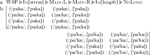
A language is a pair (Lex, ≫) of a lexicon
and an OT grammar, or equivalently the corresponding constraint ranking
≫. This definition captures the intuition that languages such as
English, Italian and Latin all consist of a specific lexicon and a specific
phonological grammar. The ingredients (ℛ, , 핉, 핊,
Gen, ) described in §2.1
thus define a typology of languages, namely the typology of all pairs
(Lex, ≫) of a lexicon Lex
together with the OT grammar corresponding to a constraint ranking
≫.
2.3 Paradigms
A paradigm specifies the surface realisation of certain combinations of a root and a suffix meaning. A generic paradigm is denoted by π. Thus the identity π(Mm)=Xx says that the meaning combination Mm of the root meaning M and the suffix meaning m is realised as the surface concatenation Xx according to the paradigm π. This definition captures the usual notion of paradigm, such as the Latin paradigm in (8). Root meanings are listed by row, suffix meanings are listed by column, the top left entry [akwa] provides the surface realisation of the meaning combination WATERnom.
-
(8)

A paradigm π is consistent with a language (Lex, ≫) provided it satisfies the crucial condition (9). The lexicon Lex maps the root meaning M to some underlying root morpheme A=Lex(M) and the suffix meaning m to some underlying suffix morpheme a=Lex(m). We can then concatenate this root A with this suffix a and feed the resulting concatenation Aa to the OT grammar G≫ corresponding to the ranking ≫, which will return a certain surface concatenation Xx. Condition (9) says that the surface concatenation Xx thus obtained is exactly the one assigned by the paradigm π to the meaning combination Mm we started from.
-
(9)

To illustrate, Latin is consistent with the paradigm (8) because its lexicon maps the root meaning WATER to /akw-/ and the suffix meaning nom to /-a/, and its phonology allows the resulting underlying concatenation /akwa/ to surface faithfully, as in the top left entry in (8). To give another example, the paradigm (10) is consistent with the language (Lex, ≫), corresponding to the lexicon Lex in (6) and the grammar G≫ in (7). In fact, the root meaning BOY corresponds to the underlying root /pa/ according to the lexicon Lex, the suffix meaning nom corresponds to the underlying form /ka/, and the resulting underlying concatenation /paka/ surfaces as [ˈpaka] according to the grammar G≫, as in the top left entry of the paradigm in (10).
-
(10)

A paradigm is, essentially, a collection of surface concatenations Xx, Yy, …, annotated with the corresponding root and suffix meanings. These meanings reveal whether two different surface concatenations Xx and Yy are the surface realisations of two meaning combinations Mm and M&capsmfrown;, which share, say, the same root meaning M. If the surface forms X and Y are different, then we know that the underlying form (whatever it is) assigned by the lexicon to the shared root meaning M undergoes some alternation when it surfaces in the context of one or both of the two suffixes m and &capsmfrown;. As an example, we have noted above that stress of the morpheme corresponding to the root meaning BOY alternates according to the grammar (7), depending on whether that root is concatenated with nom or dat. Paradigm (10) encodes this alternation, because the first and third entries in the top row show that the root surfaces with a different stress in the two concatenations. In other words, a paradigm is a way to encode information on the alternations enforced by the corresponding grammar, without revealing the underlying forms assigned by the corresponding lexicon.
2.4 The learning problem
A child acquiring English, Italian or Latin is exposed to a sequence of surface concatenations Xx, Yy, … . Because of the assumption that surface roots and suffixes belong to disjoint sets of morphemes, the learner can parse any surface concatenation Xx into its root X and its suffix x. Assume that the context of utterance provides the child with enough cues to reconstruct the root meaning M, corresponding to the surface root X, and the suffix meaning m, corresponding to the surface suffix x. The child thus effectively has access to pairs (Mm, Xx) of a root/suffix meaning combination Mm and its surface realisation Xx. The collection of these training pairs is a paradigm consistent with the native phonology. These considerations motivate the problem of learning languages from paradigms, explicitly stated in (11).
-
(11)

From the generative perspective, the learner has full knowledge of the underlying typology of languages, as stated in (11a.i). As motivated above, the data fed to the learner consist of some paradigm generated by some language in the typology, as stated in (11a.ii). Equivalently, the learner is provided with information concerning the alternations without being shown the underlying forms. The target language is one of possibly many languages which are consistent with the paradigm. As a first attempt at solving the problem of reconstructing the target language, the learner thus looks for a language consistent with the input paradigm, as stated in (11b).Footnote 4 A specific instance of the learning problem (11) is provided in (12). The language (Lex, ≫), consisting of the lexicon Lex in (6) and the ranking ≫ in (7a), is a solution of this specific instance of the problem of learning languages from paradigms.
-
(12)

2.5 Some simplifying assumptions
To start from the simplest possible case, Tesar tackles the learning problem in (11) under the restrictive assumptions in (13) on the underlying typology. Morphemes are assumed to have the simplest possible shape, i.e. they consist of a single segment. The phonology is assumed to be feature-based, and the features are assumed to be as simple as possible.
-
(13)

To illustrate, note that the Paka typology defined in §2.1 satisfies these simplifying assumptions. In fact, underlying root and suffix morphemes effectively consist of a single segment, namely the vowel (the consonant serves no other purpose than to distinguish roots from suffixes). And the set Φ of relevant features consists of the two features [length] and [stress], which are both binary and total, and furthermore independent (all four combinations of values are instantiated).Footnote 5
2.6 How to measure the efficiency of a learner
Certain instances of the learning problem (11) are ‘larger’ than others: they have more features, more morphemes, more constraints, a larger input paradigm, and so on. Larger instances require the learner to ‘do more work’, namely to perform a larger number of steps. The time complexity of a learner is the rate at which the number of steps required by the learner grows with the size of the instances. If it grows slowly (i.e. polynomially), then the learner is efficient, and can tackle instances of the problem which have a realistic size. Whether a learner qualifies as efficient depends of course on how the size of the instances of the problem is measured. In this subsection, I consider two different measures of the size of the instances of the problem of learning languages from paradigms, which lead to a generous and a (more) demanding notion of efficiency.
2.6.1 A generous definition of efficiency
According to one approach, a learner should be allowed enough time to scan
the morpheme sets ℛ and to find a
good underlying morpheme for each meaning, and thus assemble a lexicon. The
number of steps which a learner is allowed to make should thus depend on the
number of morphemes
(|ℛ|+||), leading to
definition (14).Footnote
6
-
(14)

Letting the permitted number of steps depend on the number of
morphemes
|ℛ|+|| as in (14) gives the learner enough time to
inspect the input paradigm π. Furthermore, it gives enough time
to scan any candidate set, which is crucial, given that no currently
available OT ranking algorithm succeeds without scanning all the candidates
(in the worst case). On the other hand, letting the permitted number of
steps depend on the number of morphemes does not make the problem trivial.
In fact, the number of lexicons is factorial in the number of morphemes
(because lexicons are bijections between meanings and an equal number of
morphemes). Thus, allowing the learner the time to scan all the morphemes
does not afford it enough time to exhaustively scan the
typology of languages: a brute-force search is not efficient.
2.6.2 A more demanding definition of efficiency
In §2.5, the learning setting was simplified by assuming that the
underlying root and suffix morphemes consist of single segments which are
distinguished by a certain set Φ of binary, total and independent
features. Within this feature-based framework, Tesar suggests that the
number of steps that a learner is allowed to make should depend on the
number of features |Φ|, rather than on the
number of morphemes
|ℛ|+||, leading to
definition (15). The difference
between the two formulations in (14) and (15) is
substantial, because the number of morphemes grows exponentially in the
number of features. Tesar's notion of efficiency in (15) is thus more demanding than the
one in (14).Footnote
7
-
(15)

The definition in (15) must crucially allow the number of steps made by the learner to also depend on the number of entries in the input paradigm π. In fact, the input paradigm π could consist of a full 4|&phosupPHgr;| entries, in which case a learner could not even inspect the paradigm in time polynomial in the number of features. Furthermore, Tesar's definition must crucially allow the number of steps also to depend on the size of the largest candidate set. In fact, a candidate set could consist of a full 4|&phosupPHgr;| entries, in which case the learner could not inspect the candidate set in time polynomial in the number of features, and thus would not be able to tackle even a basic ranking problem (because, as noted above, no currently available OT ranking algorithm succeeds without scanning all the candidates in the worst case).Footnote 8
3 Output-drivenness
This section introduces the notion of output-drivenness. The presentation is tailored to the restrictive representational framework described in the statement of the learning problem in §2, and thus does not attempt to do justice to the theory of output-drivenness developed in Chapters 2 and 3 of Tesar's book in a much broader context.
3.1 Similarity
Recall the representational framework we are assuming. Underlying forms Aa, Bb, … and their surface candidates Xx, Yy, … are concatenations of roots A, B, … , X, Y, … and suffixes a, b, … x, y, … . To start from the simplest possible case, we assumed in (13) that each root and each suffix consists of a single segment, that these segments are characterised in terms of a certain set Φ of phonological features and that these features are all total and binary. Within this representational framework, condition (16) formalises the intuition that an underlying concatenation Aa is less similar to a surface concatenation Xx than is another underlying concatenation Bb.Footnote 9
-
(16)

To illustrate, consider again the Paka typology in §2.1. The corresponding feature set Φ consists of the two features [length] and [stress] (which are total and binary). The underlying form Aa=/ˈpaːka/ is less similar to the surface form Xx=[paˈkaː] than is the underlying form Bb=/ˈpaˈka/. In fact, condition (16) holds for the roots, because the more similar underlying root B=/ˈpa/ differs from the surface root X=[pa] in the feature [stress], as does the less similar root A=/ˈpaː/ (besides also differing in the other feature, [length]). Condition (16) holds for the suffixes as well, because the more similar underlying suffix b=/ˈka/ differs from the surface suffix x=[ˈkaː] in the feature [length], and the less similar suffix a=/ka/ also differs in that feature (besides differing in the other feature, [stress]). By analogous reasoning, the sixteen underlying forms of the Paka typology in (3) can be ordered as in (17) according to their similarity to the surface form Xx=[paˈkaː] (more similar forms are positioned above less similar ones).
-
(17)

The underlying form /paˈkaː/ is located at the top of the lattice, because it is of course the most similar underlying form to the surface form [paˈkaː], which induces the lattice. The underlying form /ˈpaːka/ is at the bottom of the lattice, because its root and suffix differ in both the features [length] and [stress] from the surface form [paˈkaː].
3.2 Output-drivenness
Output-drivenness captures the following intuition: any discrepancy between an underlying and a surface concatenation is driven by the goal of making the surface (or output) concatenation fit the phonotactics. This intuition can be elaborated as follows. Suppose that a grammar G maps a certain underlying concatenation Aa to a certain surface concatenation Xx. Intuitively, this means that Xx is phonotactically licit and that Aa is not too dissimilar from Xx according to that grammar. Consider another underlying concatenation Bb, which is more similar to Xx than Aa is. An output-driven grammar G then also maps Bb to Xx, since the phonotactic status of Xx does not depend on the underlying form, and Bb is even more similar to Xx.
-
(18)

Consider again the relative similarity of the sixteen underlying forms of the Paka typology to the surface form Xx=[paˈkaː], represented by the lattice in (17). Suppose that an output-driven grammar maps the underlying form Aa=/paːka/ to that surface form Xx=[paˈkaː]. Then it must also map to Xx=[paˈkaː] any underlying form given in bold in (19), as they are all more similar to Xx=[paˈkaː] than is Aa=/paːka/. Output-drivenness thus substantially limits the ‘freedom’ of a grammar. We will see below in §3.4 that each OT grammar in the Paka typology is guaranteed to satisfy the output-drivenness condition in (18).
-
(19)

Chain shifts and derived environment effects yield phonological mappings which are not output-driven.
3.3 Idempotency
Assume that a grammar G maps some underlying concatenation Aa to some surface concatenation Xx. This means in particular that the surface concatenation Xx is phonotactically licit according to this grammar G. Furthermore, condition (16) guarantees that Xx (construed as an underlying concatenation) is more similar to itself (construed as a surface concatenation) than to any other underlying concatenation Aa. The output-drivenness condition (18), with Xx in place of Bb, thus ensures that G maps any phonotactically licit form Xx (construed as an underlying concatenation) to itself (construed as a surface concatenation). The latter condition states that the grammar G is idempotent, a property which plays a crucial role in the literature on the acquisition of phonotactics (Hayes Reference Hayes2004, Prince & Tesar Reference Prince and Tesar2004). In other words, output-drivenness entails idempotency (but not vice versa).
3.4 Output-drivenness for OT grammars
The definition of output-drivenness in (18) is independent of the framework used to define phonological grammars. In Chapter 3, Tesar focuses on OT and addresses the following question: which constraint sets yield typologies of OT grammars which are all output-driven? Consider an OT grammar which maps the less similar underlying concatenation Aa to the surface concatenation Xx. The mapping (Aa, Xx) therefore beats the mapping (Aa, Yy) for any other surface concatenation Yy, according to the constraint ranking corresponding to that grammar. This in turn means that there is one constraint preferring the winner mapping (Aa, Xx) over the loser mapping (Aa, Yy) which is ranked above every constraint which instead prefers (Aa, Yy) over (Aa, Xx), as shown in (20).
-
(20)

Consider another underlying concatenation Bb, which is more similar to Xx than is Aa, and must therefore also be mapped to Xx, in order for output-drivenness to hold. If the top-ranked constraint in (20) is a markedness constraint M, then it does not care whether the underlying concatenation is Aa or Bb. The fact that M prefers the mapping (Aa, Xx) over the mapping (Aa, Yy) thus entails that it also prefers (Bb, Xx) over (Bb, Yy). If instead this constraint is a faithfulness constraint F, this entailment holds, provided that F satisfies condition (21).
-
(21)

The diagram in (20) can thus be updated as shown by the underlining in (22).
-
(22)

Consider now a constraint which incorrectly prefers the mapping (Bb, Yy) to the mapping (Bb, Xx). If it is a markedness constraint M, then it again also prefers (Aa, Yy) to (Aa, Xx), i.e. it is one of the constraints C 1, C 2, … ranked at the bottom of (22). If instead it is a faithfulness constraint F, the same conclusion holds, provided that the faithfulness constraint F satisfies condition (23).
-
(23)

The diagram in (22) can thus be updated as shown by the underlining in (24).
-
(24)

The ranking configuration in (24) ensures that the ranking considered ranks a constraint which prefers (Bb, Xx) to (Bb, Yy) above every constraint which instead prefers (Bb, Yy) to (Bb, Xx), so that (Bb, Xx) wins over (Bb, Yy). Since this conclusion holds for any surface concatenation Yy, the grammar considered indeed maps the more similar underlying form Bb to Xx, as desired.
Let me take stock. Suppose that every faithfulness constraint F satisfies the two conditions (21) and (23) whenever the underlying concatenation Bb is more similar to the surface concatenation Xx than is the underlying concatenation Aa. Then, any grammar corresponding to any ranking of the constraint set is output-driven, no matter what the markedness constraints are. Tesar shows in particular that Ident-type faithfulness constraints, Max and Dep satisfy these two crucial conditions (pp. 108–115). Thus, for example, every grammar in the OT typology defined by the Paka specifications is output-driven, because the set of faithfulness constraints in (5b) consists only of the two identity constraints Ident[stress] and Ident[length]. Other faithfulness constraints (including Dep[V], Max[C], the local conjunction of two Ident-type faithfulness constraints and positional faithfulness constraints) are shown by Tesar not to satisfy the two conditions in (21) and (23). These constraints have indeed been used in the OT literature to capture non-output-driven phenomena such as chain shifts and derived environment effects (see Chapter 4 for discussion and references).
4 What can output-drivenness do for the learner? The perspective of time complexity
§2 reviewed the problem of learning languages from paradigms. Tesar tackles this problem starting from the premise that ‘for language learning to be possible, the linguistic theory must have some kind of non-trivial structure … that can be exploited by a learner’ (p. 18). §3 reviewed a structural condition that could be imposed on the typology explored by the learner, namely output-drivenness. Unfortunately, this is not a typological universal: several attested phonological phenomena are not output-driven, and various faithfulness constraints indeed give rise to non-output-driven behaviour. Tesar (p. 18) nonetheless contends that ‘the definition of output-driven maps is a first cut at identifying [the] structure’ which makes learning possible. These considerations motivate the following question: what can output-drivenness do for the learner? As anticipated in §1, this section (together with the next one) addresses this question by comparing Tesar's Output Driven Learner (ODL) with Merchant's (Reference Merchant2008) Contrast Pair and Ranking Information (CPR) learner. §4.1 outlines the architecture shared by CPR and ODL, based on the idea of maintaining partial lexical and ranking information which is incremented iteratively. §4.2 (complemented by Appendix A) introduces CPR's subroutines for extracting lexical and ranking information. These subroutines are guaranteed never to make an error, but are too slow to be efficient. §4.3 (complemented by Appendix B) then introduces ODL's subroutines as a speeded-up reformulation of CPR's subroutines through output-drivenness. The implications of this speed-up for efficiency are discussed. Finally, §4.4 and §4.5 illustrate two of ODL's speeded-up subroutines in more detail, underscoring the role played by output-drivenness in their analyses.
4.1 The common architecture of CPR and ODL
4.1.1 Partial lexical information
As stated in (13), we are assuming that root and suffix morphemes consist of single segments which are distinguished by a certain set Φ of phonological features. A lexicon can thus describe the underlying segment it assigns to a certain meaning by specifying the value of each feature in that segment. To illustrate, consider again the Paka typology defined in §2.1. As noted above, its root and suffix morphemes effectively consist of single segments (the vowels) which are distinguished by the two features [length] and [stress]. The lexicon (6) can thus be specified in terms of feature-values as in (25). The two entries ‘−’ in the leftmost column specify that the underlying segment corresponding to the root meaning BOY is [−long] and [−stress], i.e. it is /pa/, as determined by (6).
-
(25)

A partial lexicon leaves some features unset for some root or suffix segments. An extreme case is that of an empty lexicon, which does not specify the value of any feature for any meaning. At the other extreme, a lexicon which specifies the value of each feature for each meaning is total. From now on, I will use the term ‘lexicon’ and the symbol Lex to refer to a lexicon which can be either partial or total. To illustrate, the lexicon in (25) is total, while that in (26) is partial, for instance because it fails to specify the value of the feature [length] for the root meaning GIRL.
-
(26)

Two lexicons are consistent provided they agree where both are specified: if a certain feature is set for a certain meaning by both lexicons, then it is set to the same value. To illustrate, the two lexicons in (25) and (26) are consistent. Finally, an underlying form Aa for a meaning combination Mm is consistent with a lexicon Lex provided it agrees with any feature specified by the lexicon: if a feature is set by the lexicon Lex for the root meaning M (for the suffix meaning m) to some value, the root morpheme A (the suffix morpheme a) has that value for that feature. To illustrate, the partial lexicon (26) is consistent with both underlying forms /paˈka/ and /paːˈka/ for the meaning combination GIRLgen, as the lexicon does not set the feature [length] for the root meaning GIRL.
4.1.2 Partial grammatical/ranking information
An OT grammar is a collection of mappings (Aa, Xx) which specify that an underlying form Aa is mapped to a surface form Xx. A partial grammar specifies the surface realisation only for some underlying concatenations. An extreme case is that of an empty grammar, which does not specify the surface realisation of any underlying concatenation. At the other extreme, a grammar which provides a mapping for each underlying concatenation is total. From now on, I will use the term ‘grammar’ and the symbol G to refer to a grammar which can be either partial or total. To illustrate, consider again the Paka typology. The grammar in (7b) is total, because it provides surface realisations for each of the sixteen underlying concatenations in (3), whereas the grammar in (27) is partial, because it fails to provide surface realisations for the underlying concatenations /pakaː/, /ˈpaˈka/, etc.
-
(27)

Two grammars are consistent provided there exists at least one ranking which is consistent with both. This entails in particular that, if the two grammars both provide a surface realisation for a certain underlying concatenation, they provide the same surface realisation. Thus the grammar in (7b) and the partial grammar in (27) are consistent. Finally, a mapping (Aa, Xx) of an underlying concatenation Aa to a surface concatenation Xx is consistent with a grammar G provided there exists at least a ranking which is consistent with both, namely it maps Aa to Xx and furthermore maps the underlying concatenation Bb to the surface concatenation Yy for every mapping (Bb, Yy) prescribed by the grammar G. Thus the partial grammar in (27) is consistent with the mapping (/pakaː/, [ˈpaka]), because both that partial grammar and the mapping are consistent with the ranking in (7a).
4.1.3 Iteratively boosting partial lexical and partial ranking information
The learning problem in (11) asks for a language consistent with a given paradigm. A language consists of a lexicon and an OT grammar, or equivalently the corresponding ranking. A natural approach to this learning problem is to maintain partial lexical information and partial grammatical information and to increment them iteratively by ‘boosting’ one type of partial information with the other. This idea is formalised in the algorithmic scheme in (28). The learner reads the input paradigm π, which is provided with an instance of the learning problem (line 1). It maintains lexical information in the form of a current (possibly partial) lexicon Lex and grammatical information in the form of a current (possibly partial) grammar G. They are initialised to the empty lexicon and the empty grammar (line 2). They are then updated by boosting one against the other. On the one hand, the learner tries to extract new grammatical information (i.e. to add new mappings to its current grammar G), using the lexical information encoded in its current (possibly partial) lexicon Lex (line 4). On the other hand, the learner tries to extract new lexical information (i.e. to set some feature still unspecified by the current lexicon Lex) using the ranking information encoded in the current (possibly partial) grammar G (line 5). These two steps are repeated until no new lexical or grammatical information can be extracted from the input paradigm (line 6). The algorithm then returns its current lexicon Lex and its current grammar G (line 7). The returned lexicon Lex and the returned grammar G can of course be partial. The learner is deemed correct as long as any total lexicon Lex total consistent with the returned lexicon Lex and any total grammar G total consistent with the returned grammar G yield a language (Lex total, G total) which is consistent with the input paradigm π, and thus solves the instance of the problem the learner has been trained on.
-
(28)
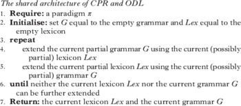
Both Merchant's (Reference Merchant2008) CPR and Tesar's ODL subscribe to this idea of iteratively boosting partial lexical and grammatical information against each other. The algorithmic scheme (28) thus distils their shared architecture. I now turn to the subroutines used by CPR and ODL at lines 4 and 5 for extracting ranking and lexical information.
4.2 CPR's slow subroutines
CPR's subroutines are based on three core ideas: join, inconsistency detection and contrast pairs. This subsection (complemented by Appendix A) offers a quick sketch of these ideas. Merchant develops a new subroutine for extracting grammatical/ranking information. The intuitive idea is as follows (see Appendix A: §3 for details). The partial lexical information encoded in the current lexicon Lex reduces the range of possible underlying forms for a certain meaning combination Mm to those consistent with Lex. The subroutine thus considers all mappings of all consistent underlying forms to the surface form of Mm provided by the paradigm. It then extracts any ranking information which is shared across all such mappings. Shared ranking information is extracted through a novel technique based on the notion of join. The technique is provably optimal, in the sense that it extracts as much ranking information as possible.
CPR's subroutine for extracting lexical information is based on the classical method of inconsistency detection (Kager Reference Kager1999, Tesar et al. Reference Tesar, Alderete, Horwood, Nishitani and Prince2003, Tesar Reference Tesar2006, among many others). The intuitive idea is as follows (see Appendix A: §5 for details). A certain feature is set to a certain value for a certain meaning combination Mm by detecting the fact that the opposite value is inconsistent with the current ranking information, in the sense that there is no ranking consistent with the current ranking information which is able to map an underlying form for Mm with the opposite value to the surface form for Mm provided by the paradigm. Both the subroutine for extracting ranking information through the join and the subroutine for extracting lexical information through inconsistency detection come with correctness guarantees: if the current lexical and ranking information is correct, the extended lexical information and the extended ranking information returned by these subroutines are correct as well.
These two subroutines for extracting ranking and lexical information can be applied not only to a single entry in the paradigm corresponding to a single meaning combination Mm, but also to a contrast pair, i.e. a pair of meaning combinations which share either the root meaning (a pair such as Mm and M&capsmfrown;) or the suffix meaning (a pair such as Mm and &Mfrown;m). Various authors (including Alderete et al. Reference Alderete, Brasoveanu, Prince and Tesar2005 and Merchant & Tesar Reference Merchant and Tesar2008) have pointed out that the subroutine for extracting lexical information through inconsistency detection extracts more information when applied to contrast pairs than when applied to individual paradigmatic entries. The intuitive idea is as follows (see Appendix A: §6 for details). Contrast pairs (not single entries) are indeed the smallest data units able to display morphophonemic alternations. A learner which extracts lexical information by only looking at a single entry at the time is thus effectively ignoring the alternations encoded in the paradigm, and is therefore bound to fail. This intuition carries over to Merchant's new subroutine for extracting ranking information, which is indeed boosted by being applied to contrast pairs rather than to single paradigmatic entries (see Appendix A: §4 for details).
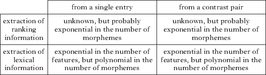
The crux of CPR's subroutines is their time complexity. Recall from §2.6 that the time complexity of an algorithm for learning languages from paradigms can be measured either in terms of the number of morphemes (leading to a laxer notion of efficiency) or in terms of the number of features (leading to a more demanding notion of efficiency). The time complexity of CPR's subroutines is summarised in Table I.
Time complexity of CPR's subroutines.

Merchant's subroutine for extracting ranking information based on the join relies on the operation of fusional closure. Unfortunately, there are no results which I am aware of on the efficient computation of the fusional closure. The time complexity of Merchant's subroutine for extracting ranking information is thus unknown. But the subroutine is most likely not efficient, no matter how efficiency is defined and no matter whether the subroutine is applied to a single entry of the paradigm or to a contrast pair, as summarised in the first row of Table I. The efficiency of the subroutine for extracting lexical information based on inconsistency detection depends on how its time complexity is measured. In fact, the subroutine is efficient relative to the laxer measure of time complexity (in terms of the number of morphemes), but not relative to the more demanding measure of time complexity (in terms of the number of features), no matter whether the subroutine is applied to a single entry in the paradigm or to a contrast pair, as summarised in the second row of Table I.
4.3 ODL's speeded-up subroutines through output-drivenness
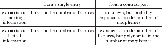
What is the effect of output-drivenness on the efficiency of the subroutines reviewed in the preceding subsection? The most spectacular implication of output-drivenness is a huge speed-up of Merchant's subroutine for extracting ranking information from a single entry in the paradigm. That subroutine requires the computation of the join, and is thus (most plausibly) inefficient, no matter how efficiency is defined, as indicated in the top left cell of Table I. Output-drivenness circumvents the computation of the join, leading to a restatement of the subroutine, whose time complexity grows only very slowly (i.e. linearly) with the number of features, as stated in the top left cell of Table II. In other words, the subroutine becomes efficient. And efficiency holds even relative to the strictest of the two measures of time complexity introduced in §2.6.
Time complexity of ODL's subroutines.

Tesar's subroutine for extracting ranking information from a single meaning concatenation using output-drivenness is presented in §4.4, together with an analysis of its time complexity and correctness, which highlights the role of output-drivenness. Appendix B: §1 explains the equivalence between Tesar's and Merchant's subroutines.
Output-drivenness also provides a substantial speed-up of the subroutine for extracting lexical information from a single entry in the paradigm through inconsistency detection. As indicated in the bottom left cell of Table I, that subroutine is only efficient relative to the laxer measure of time complexity (in terms of the number of morphemes), not the stricter measure (in terms of the number of features). Output-drivenness allows a restatement of this subroutine whose time complexity grows only very slowly (i.e. linearly) with the number of features, as stated in the bottom left cell of Table II. In other words, the subroutine becomes efficient relative to the strict measure of time complexity as well. Tesar's subroutine for extracting lexical information from a single meaning concatenation using output-drivenness is presented in §4.5, together with an analysis of its time complexity and correctness which highlights the role of output-drivenness. Appendix B: §2 explains the connection between Tesar's subroutine and inconsistency detection.
Tesar discusses in detail how output-drivenness can be used to reformulate the subroutine for extracting lexical information from contrast pairs through inconsistency detection. This discussion is rather more technical, and is therefore relegated to Appendix B: §3. The upshot of this discussion is the following. Output-drivenness does not improve the time complexity of the subroutine, which remains inefficient relative to the stricter measure of time complexity (in terms of the number of features), as stated in the bottom right cell of Table II. Output-drivenness can nonetheless be used to construct a variant of this subroutine which is faster, although weaker.
Merchant's subroutine for extracting ranking information requires the time-consuming computation of the join, no matter whether the subroutine is applied to a single entry of the paradigm or to a contrast pair. As noted above, output-drivenness allows a huge reduction of time complexity when the subroutine is applied to a single entry, because output-drivenness effectively allows us to circumvent the computation of a join. Tesar does not discuss the case where Merchant's subroutine for extracting ranking information is applied to a contrast pair. In this case, it seems to me that there is no way around the join, as explained in Appendix B: §4. If this conclusion is correct, the time complexity cannot be reduced through output-drivenness, and the subroutine remains inefficient, as stated in the top right cell of Table II.
A comparison of Tables I and II shows that output-drivenness has a substantial effect on time complexity when lexical and ranking information is extracted from a single entry in the paradigm, but also that output-drivenness unfortunately falls short when lexical and ranking information is extracted from a contrast pair. Table II furthermore raises the following question: does the learner really need the full power afforded by Merchant's subroutine for extracting ranking information from contrast pairs? Or can the learner content itself with the ranking information that can be extracted from a single entry at a time? To the best of my knowledge, this question is currently open.Footnote 10 It seems to me that this is crucial for the prospects of output-drivenness. If it turns out that the ranking information extracted from single entries suffices, then we can dismiss the bad news in the top right cell of Table II, and conclude that output-drivenness is indeed the structural assumption needed by the learner in order to achieve efficiency. If, instead, the additional ranking information provided by contrast pairs is needed, then output-drivenness will plausibly have to be supplemented with additional structural assumptions, able to yield a significant improvement in the top right cell of Table II.
4.4 Extracting ranking information using output-drivenness
4.4.1 Description of the subroutine
The subroutine Extract Ranking Information defined in (29) takes as input some partial ranking information in the form of a partial grammar G, some lexical information in the form of a (possibly partial) lexicon Lex and a paradigm π (line 1). It extends that ranking information by adding to the partial grammar G an additional mapping, as follows. The subroutine considers a certain meaning combination Mm (line 2). It reads off the paradigm π the surface realisation Xx of that meaning combination (line 3). It then constructs the underlying concatenation Bb as follows (line 4). If a feature is set by the input lexicon Lex to a certain value for the root meaning M or for the suffix meaning m, then the underlying root B or suffix b has that value for the feature; otherwise, the underlying root B or suffix b has the same value for the feature as the surface root X or suffix x. The subroutine then updates the current partial grammar G by adding the mapping (Bb, Xx) of the underlying concatenation Bb just constructed to the surface realisation Xx provided by the paradigm (line 5). The grammar thus updated is then returned (line 6).
-
(29)
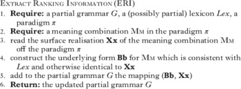
4.4.2 Analysis of the subroutine
The time complexity of ERI is controlled by the time required to execute line
4, which in turn grows only linearly with the number of features used to
define the root and suffix segments. The subroutine is therefore efficient
even relative to the more demanding notion of efficiency introduced in
§2.6.2. The following straightforward lemma uses
output-drivenness to show that ERI is also correct. 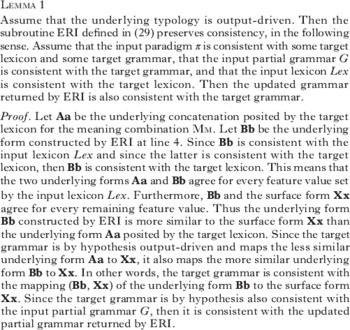
Appendix B: §1 develops the analysis of ERI further. It shows that ERI is equivalent to Merchant's (Reference Merchant2008) subroutine for the extraction of ranking information through the notion of join (Tesar does not point out this equivalence). Crucially, Merchant's subroutine is optimal (in that it extracts as much ranking information as possible), although, unfortunately, not efficient. Output-drivenness thus allows ERI to inherit the optimality of Merchant's subroutine, while affording a huge gain in time complexity.
4.4.3 First example
Consider the example in (12) of the problem of learning languages from paradigms, whereby the underlying typology is the Paka typology defined in §2.1 and the paradigm is the one in (10), generated by the lexicon in (6) and the OT grammar in (7). Suppose that the ERI subroutine is fed the empty input grammar G and the empty lexicon Lex (line 1), and that it focuses on the meaning combination BOYnom (line 2). ERI then reads off paradigm (10) the surface realisation Xx=[ˈpaka] of that meaning combination (line 3), and constructs the underlying form Bb, which is identical to that surface form Xx but for the features set in the input lexicon Lex (line 4). Since Lex is empty, ERI constructs the completely faithful underlying form Bb=/ˈpaka/. ERI then faithfully adds to the empty grammar G the mapping (Bb, Xx)=(/ˈpaka/, [ˈpaka]) of the underlying form /ˈpaka/ to [ˈpaka]. After running ERI iteratively on all meaning combinations, it finally returns the partial grammar in (30a), which contains the four forms which appear in the paradigm, faithfully mapped to themselves. This partial grammar is equivalent to the ranking conditions in (30b).
-
(30)

The application of ERI with an empty input lexicon Lex is also called phonotactic learning (§5.6.2 of Tesar's book): since the lexicon is empty, the learner is extracting ranking information from the simple fact that the surface forms [ˈpaka], [paˈka], [paˈkaː] and [ˈpaːka] appear in the paradigm, i.e. are all phonotactically licit.
4.4.4 Second example
Suppose now that ERI is fed the partial grammar G in (30) and the partial lexicon Lex in (31), which sets values for the feature [length] (line 1). Suppose furthermore that it focuses on the meaning combination DOGdat (line 2). ERI then reads off paradigm (10) the surface realisation Xx=[ˈpaka] of that meaning combination (line 3), and constructs the underlying form Bb=/ˈpakaː/ (line 4), which is identical to the surface form Xx=[ˈpaka] but for the features set in the current lexicon for the root DOG (none) and the suffix dat (i.e. [length], which has been set to +).
-
(31)

ERI then adds to the empty grammar G the mapping (Bb, Xx)=(/ˈpakaː/, [ˈpaka]) of the just constructed underlying form /ˈpakaː/ to the surface form [ˈpaka] (line 6), and returns the updated grammar (32a). This partial grammar is equivalent to the ranking conditions in (32b).
-
(32)

This example illustrates how ERI is able to extract new non-phonotactic ranking information from a lexicon such as (31), which is partial and thus sets only a few feature values.
4.5 Extracting lexical information using output-drivenness
4.5.1 Description of the subroutine
The subroutine Extract Lexical Information defined in (33) takes as input some lexical information in the form of a partial lexicon Lex, some ranking information in the form of a (possibly partial) grammar G and a paradigm π (line 1). The subroutine considers a certain meaning combination Mm (line 2). And it focuses on some feature ϕ which is unset according to the input partial lexicon Lex (line 3). For concreteness, I am assuming here that the feature ϕ is unset for the root meaning M (the case where it is unset for the suffix meaning m is completely analogous). The goal of the subroutine is to extend the input partial lexicon Lex by trying to set the feature ϕ for the root meaning M. The subroutine reads off the paradigm π the surface realisation Xx of that meaning combination Mm (line 4). And it considers the underlying concatenation Bb which is consistent with the input lexicon Lex and is otherwise identical to the surface concatenation Xx, but for the fact that the underlying root B and the surface root X have opposite values for the feature ϕ (line 5). If the input grammar G is not consistent with the mapping (Bb, Xx) of this underlying concatenation Bb to the surface concatenation Xx (line 6), then the subroutine concludes that it is not possible to set the feature ϕ for the root meaning M to the opposite value from the one it surfaces with in X. The subroutine thus updates the lexicon by setting the feature ϕ for the root meaning M equal to the value it surfaces with in X (line 7). The lexicon thus updated is then returned (line 9).
-
(33)
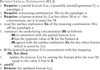
4.5.2 Analysis of the subroutine
The time complexity of the subroutine ELI is controlled by the time required
to execute line 4, which in turn grows only linearly with the number of
features used to define the root and suffix segments. The subroutine is
therefore efficient even relative to the more demanding notion of efficiency
introduced in §2.6.2. The following straightforward lemma uses
output-drivenness to show that ELI is also correct. 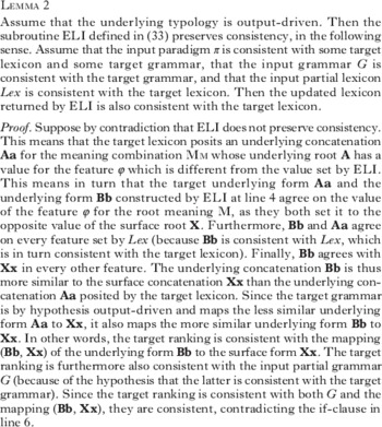
Appendix B: §2 further develops the analysis of ELI. It shows that it is equivalent to the classical strategy of inconsistency detection. Crucially, the time complexity of inconsistency detection is exponential in the number of features. Output-drivenness thus affords a substantial reduction of time complexity.
4.5.3 Example
Consider again instance (12) of the problem of learning languages from paradigms. Suppose that ELI is fed the empty lexicon Lex and the input grammar G in (30) obtained above through phonotactic learning (line 1). Suppose that it considers the meaning combination BOYnom (line 2) and that it focuses on the feature ϕ=[length], not set by the input lexicon Lex for the root meaning BOY (line 3). ERI then reads off paradigm (10) the surface realisation Xx=[ˈpaka] of this meaning combination (line 4). The target feature ϕ=[length] surfaces with the value ‘−’ in the surface root X=[ˈpa]. ELI thus tries to rule out the hypothesis that this feature ϕ=[length] is set to the opposite value ‘+’ in the underlying root for BOY. To this end, ELI constructs the underlying concatenation Bb, which is consistent with Lex and otherwise identical to the surface realisation Xx, but for the feature ϕ=[length] for the root BOY, which is set to the value ‘+’ (line 5). Since Lex is empty, this is the underlying concatenation Bb=/ˈpaːka/. ELI then checks whether the input partial grammar G is consistent with the mapping (Bb, Xx)=(/ˈpaːka/, [ˈpaka]) of the just constructed underlying concatenation /ˈpaːka/ to the surface concatenation [ˈpaka] (line 6). Consistency fails. In particular, this mapping requires the markedness constraint NoLong to be ranked above the faithfulness constraint Ident[length] in order for (/ˈpaːka/, [ˈpaka]) to win over (/ˈpaːka/, [ˈpaːka]). This ranking is inconsistent with the ranking in (30b) expressed by the input grammar G. ELI thus updates the current empty lexicon by setting the feature [length] for the root meaning BOY to be the same as the value ‘−’ it surfaces with in [ˈpaka], so that the updated lexicon is as in (34).
-
(34)

This step can be summarised as follows. The paradigm contains forms with a long vowel. This means that long vowels are phonotactically licit (at least when stressed). Phonotactic learning has been able to learn that, namely to learn that Ident[length] needs to be ranked above NoLong, as in (30). An underlying (stressed) long vowel thus cannot be shortened, hence the inconsistency of the mapping (/ˈpaːka/, [ˈpaka]) considered by ELI.
5 What can output-drivenness do for the learner? The perspective of correctness
Suppose that ODL is trained on an input paradigm which is consistent with some target
language (Lex
tar, ≫tar) in the
underlying typology.Footnote
11
ODL initialises its current lexicon Lex to the empty
lexicon and its current grammar G to the empty grammar. The initial
lexicon Lex, being empty, is trivially consistent with the target
lexicon Lex
tar. Furthermore, the initial grammar
G, being empty, is trivially consistent with the grammar
corresponding to the target ranking ≫tar. ODL then
successively applies the subroutines ERI, ELI and their restatements in terms of
contrast pairs, for a number of iterations. The analyses of these subroutines
provided above in §4.4 and §4.5 (as well as in Appendix B:
§3) show that each of these subroutines preserves consistency: if the
lexicon and grammar provided as input to these subroutines are consistent with the
target lexicon Lex
tar and the target ranking
≫tar, then the updated partial lexicon and the updated
grammar returned by these subroutines are also consistent with the target lexicon
Lex
tar and the target ranking
≫tar. In conclusion, the current lexicon and the current
grammar entertained by ODL are initially consistent with
(Lex
tar, ≫tar) and stay
consistent throughout, leading to the following result. 
This theorem is partly good and partly bad news. The good news is that ODL is prudent: Theorem 1 ensures that ODL is always consistent with some target grammar. And prudence guarantees safe choices: ODL never sets a feature incorrectly in the current lexicon or adds an incorrect mapping to the current grammar. The bad news is that ODL is too prudent: Theorem 1 says that ODL is not satisfied with being consistent with one target language, but actually insists on being consistent with all of them. And excessive prudence hinders success: it is easy to formally single out cases where ODL is bound to fail because of its excessive prudence. The rest of this section elaborates on this point.
Tesar shows that when ODL is trained on the instance in (12) of the problem of learning languages from paradigms, the lexicon returned by ODL fails to set the value of the feature [length] for the two suffixes nom and acc. This is not crucial, since those feature values are not contrastive. In other words, there are four different languages (Lex&phosuptard1;, ≫tar), (Lex&phosuptard2;, ≫tar), (Lex&phosuptard3;, ≫tar) and (Lex&phosuptard4;, ≫tar) in the Paka typology which are consistent with the paradigm, and thus count as target languages. They have the same ranking, and only differ in how their four lexicons set the value of the feature [length] for the two suffixes nom and acc (two values × two suffixes gives four possibilities). Theorem 1 explains why ODL leaves those two feature values unset. Indeed, suppose there existed a run of ODL where the algorithm ended up setting those two feature values. For concreteness, suppose that ODL happened to set them as Lex&phosuptard1;. The final lexicon learned by ODL would then be inconsistent with the other three target lexicons Lex&phosuptard2;, Lex&phosuptard3; and Lex&phosuptard4;. This is forbidden by Theorem 1: the final lexicon learned by ODL must be consistent with all four of these target lexicons, and thus must leave unset any feature value where they disagree. In other words, when there are different target languages, ODL refuses to choose one over the other, and prudently abstains from making any move that would lead to an inconsistency with any of the target languages.
In the case of the Paka language considered here, the failure of ODL to set the value of the feature [length] for the suffixes nom and acc creates no problems: the partial lexicon returned by ODL can be completed by setting the two missing values at random. Yet, now that we have understood why ODL fails to set those two values, it is easy to imagine variants where ODL's failure to set some values does lead to trouble. Suppose that the paradigm that ODL is trained on is consistent with two target languages (Lex&phosuptard1;, ≫tar) and (Lex&phosuptard2;, ≫tar), which have different lexicons Lex&phosuptard1; and Lex&phosuptard2;, but (to keep things simple) share the ranking ≫tar. Suppose that the two target lexicons Lex&phosuptard1; and Lex&phosuptard2; differ in particular in the way they set a certain feature ϕ for a certain morpheme, say the root meaning M. This is the same case as, for example, the feature [length] and the morpheme nom. Yet suppose that there is some other morpheme, say another root &Mfrown; (possibly equal to M), and some other feature ψ (possibly equal to ϕ), such that consistency with the input paradigm requires the value assigned to feature ψ for &Mfrown; to crucially depend on the value assigned to feature ϕ for M. The two lexicons Lex&phosuptard1; and Lex&phosuptard2; will thus also necessarily differ in the value they assign the feature ψ for &Mfrown;. Again, when ODL is trained on this paradigm, it will fail to set the value of the feature ϕ for M and the value of the feature ψ for &Mfrown;, because it would otherwise be inconsistent with one of the two target lexicons, in contradiction of Theorem 1. Yet in this case ODL has stopped short of succeeding. In fact, because of the correlation between the two feature values for the two morphemes, these values which ODL has failed to learn cannot be set at random; they are a crucial component of the learning task.
At this point, two crucial questions arise, which unfortunately I have to leave open. The first is the following: is it possible to guarantee that ODL succeeds at least in the benign cases where the ‘pathologies’ just described do not hold? More explicitly, consider the case of a paradigm π which is consistent with a single language, so that ODL's excessive prudence cannot lead into trouble. Is it possible to guarantee that ODL succeeds in this benign case? The second question is the following: is it possible to construct phonologically plausible typologies which yield paradigms consistent with multiple languages where ODL's excessive prudence leads to trouble in the way just characterised formally? Or is it instead the case that such cases are hard to come by in natural language phonology? Whatever the answer to this question, it changes nothing for the importance of Tesar's work. If it turns out that no such cases are attested, this match between the typology of what is attested and the restrictions on what is learnable will provide exciting evidence in favour of ODL. If, instead, it turns out that such cases are well instantiated, then we will have made substantial progress, by understanding the shortcomings of ODL's reliance on inconsistency detection. And this will only have been made possible by the kind of careful and sophisticated computational work reported in Tesar's book.