1 Introduction
Nanoparticles of various sizes and shapes are employed in many technologies (Henry & Chen Reference Henry and Chen2008; Janjua et al. Reference Janjua, Nudurupati, Singh and Aubry2011; Radhakrishnan et al. Reference Radhakrishnan, Yu, Eckmann and Ayyaswamy2017). In certain applications, it is important to predict the diffusivity and the trajectory of the particle in a fluid medium close to confining boundaries where hydrodynamic interactions with the wall gain prominence. The fluid medium itself may be stationary or flowing.
In targeted drug delivery, for example, ligand functionalized nano-sized particles, or nanocarriers (NCs) are commonly used to deliver drugs to specific locations inside the vasculature. The dynamics of these particles in a confined environment, such as in a narrow blood vessel, is governed by a complex interplay between the hydrodynamic forces, Brownian interactions, wall effects and adhesive interactions of the ligands with specific receptors expressed on the vessel wall. The magnitude of each of these effects is governed by a number of factors including the size and the shape of the NC, the size of the vessel, the flow rate, the hematocrit density and the expression levels of the receptor molecules on the vascular surface (Ayyaswamy et al. Reference Ayyaswamy, Muzykantov, Eckmann and Radhakrishnan2013). Our study also has applications in the microrheology of simple and complex fluids where the frequency dependent complex shear modulus of individual particles is used to measure the local rheological properties of the material. See, for example, Waigh (Reference Waigh2005), Cicuta & Donald (Reference Cicuta and Donald2007), Squires & Mason (Reference Squires and Mason2010a ,Reference Squires and Mason b ) and Gómez-González & del Álamo (Reference Gómez-González and del Álamo2016) for details.
Here, we are concerned with the effects of the shape (which is taken to be a spheroid) and the confinement on the dynamics of the NC. These are of particular interest in targeted drug delivery where as compared to spherical NCs, spheroidal NCs have been shown to have a higher efficacy of binding to the cell (Champion & Mitragotri Reference Champion and Mitragotri2006; Shah et al. Reference Shah, Liu, Hu and Gao2011; Liu, Shah & Tan Reference Liu, Shah and Tan2012; Dasgupta, Auth & Gompper Reference Dasgupta, Auth and Gompper2013). The bulk medium, in this study, is considered to be a Newtonian incompressible fluid in a cylindrical vessel. When pressure gradients are present, the base flow is taken to correspond to a weak Poiseuille (parabolic) profile.
Numerical simulations of a finite-sized ellipsoid immersed in a fluid medium have been previously carried out using various methods, such as the Stokesian dynamics method (Wakiya Reference Wakiya1957), the finite element method (Sugihara-Seki Reference Sugihara-Seki1996; Xu & Michaelides Reference Xu and Michaelides1996; Glowinski et al. Reference Glowinski, Pan, Hesla, Joseph and Périaux2001; Swaminathan, Mukundakrishnan & Hu Reference Swaminathan, Mukundakrishnan and Hu2006), the boundary integral method (Hsu & Ganatos Reference Hsu and Ganatos1989), the Lagrange-multiplier-based fictitious domain schemes (Glowinski et al. Reference Glowinski, Pan, Hesla, Joseph and Périaux2001) and the lattice Boltzmann method (LBM) (Ding & Aidun Reference Ding and Aidun2000; Xia et al. Reference Xia, Connington, Rapaka, Yue, Feng and Chen2009; Huang, Yang & Lu Reference Huang, Yang and Lu2014). However, corresponding studies for a nano-sized ellipsoid are unavailable at present. For nano-sized particles, thermal effects should be considered. To account for the effects of the thermal fluctuations on a mechanical system, one can add the thermal force terms to the governing equations of the system based on the formulations of non-equilibrium statistical mechanics (Kubo Reference Kubo1966). In order to achieve thermal equilibrium, the spatial and temporal correlations in these systems should satisfy a balance between the thermal random force and the dissipation of the system as required by the fluctuation–dissipation theorem (Kubo Reference Kubo1966). To add the thermal force describing the Brownian motion of a particle immersed in a fluid, we adopt the fluctuating hydrodynamic approach (Landau & Lifshitz Reference Landau and Lifshitz1987), where a stochastic stress is added to the stress tensor in the fluid momentum equation. Although the particle Reynolds number is very small, the presence of thermal effects requires a treatment of the full Navier–Stokes equations together with the random stress tensor in the problem formulation. Previously, such simulations have only been carried out for a spherical NC by employing the finite volume method (Sharma & Patankar Reference Sharma and Patankar2004; Donev et al. Reference Donev, Vanden-Eijnden, Garcia and Bell2010), LBM (Ladd Reference Ladd1993, Reference Ladd1994a ,Reference Ladd b ; Patankar Reference Patankar2002; Adhikari et al. Reference Adhikari, Stratford, Cates and Wagner2005; Dünweg & Ladd Reference Dünweg, Ladd, Holm and Kremer2009; Nie & Lin Reference Nie and Lin2009), the stochastic Eulerian–Lagrangian method (Atzberger Reference Atzberger2011) and the stochastic arbitrary Lagrangian–Eulerian (ALE) method (Uma et al. Reference Uma, Swaminathan, Radhakrishnan, Eckmann and Ayyaswamy2011).
For an ellipsoidal particle, however, there are special requirements that have to be satisfied based on its shape. We employ quaternions to describe the instantaneous orientation of the ellipsoid (Chou Reference Chou1992; Kuipers Reference Kuipers1999; Swaminathan et al. Reference Swaminathan, Mukundakrishnan and Hu2006). We resolve both the translational and the rotational motions of the NC using the arbitrary Lagrangian–Eulerian finite element technique (Hu, Patankar & Zhu Reference Hu, Patankar and Zhu2001), for which the unstructured finite element mesh is generated using the Delaunay–Voronoi method (George Reference George1991). The fluctuation–dissipation theorem is satisfied by discretizing the hydrodynamic equations in terms of the finite element shape functions based on the Delaunay triangulation (Español, Anero & Zúñiga Reference Español, Anero and Zúñiga2009). In our treatment here, the fluid is considered to be incompressible. To account for compressibility effects, as discussed in Uma et al. (Reference Uma, Swaminathan, Radhakrishnan, Eckmann and Ayyaswamy2011), the added mass of the displaced fluid should be considered along with the mass of the particle. For simulations of an ellipsoidal NC, the added masses and added moments of inertia have to be considered and these are non-trivial calculations due to their dependence on the shape and orientation of the particle. The appropriate expressions for these quantities are provided in detail in this manuscript.
For the fluctuating hydrodynamics approach, a large number of realizations are required to develop adequate statistics of the dynamics, and this is computationally expensive. Under certain conditions, the relaxation behaviour of the velocity autocorrelations may also be obtained in the absence of the imposed random stress tensor. This procedure, the deterministic method, is based on the Onsager regression hypothesis, which states that the regression of microscopic thermal fluctuations at equilibrium follows the macroscopic law of relaxation of small non-equilibrium disturbances (Onsager Reference Onsager1931a ,Reference Onsager b ). The deterministic method affords computational ease to develop relevant results with a stationary medium. The details are described in a subsequent subsection.
The paper is organized as follows. Section 2 describes the mathematical formulation of the problem, the Galerkin finite element method for solving the fluid momentum equations and the generation of the random stress tensor for a tetrahedron mesh. Section 3 presents the validations, the numerical results and the discussion. In § 4 we present the conclusions.
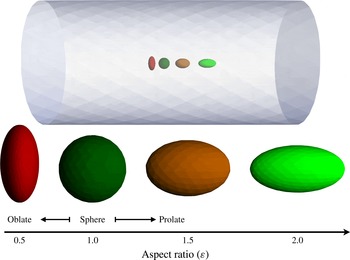
Spheroidal NCs with aspect ratio
 $\unicode[STIX]{x1D700}=0.5$
,
 $1.0$
,
 $1.5$
and
 $2.0$
at the centre of a cylindrical tube of diameter
 $D=5~\unicode[STIX]{x03BC}\text{m}$
, and oriented along the axis of the tube.

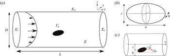
Schematic representation of (a) a spheroid bounded by a circular tube of length
 $L$
and diameter
 $D$
with a Poiseuille flow along the
 $x$
direction, (b) the dimensions of a spheroid denoted by
 $a$
,
 $b$
and
 $c$
. Panel (c) shows the various length scales in the system: the proximity of the particle from the wall boundary described either in terms of its radial distance
 $r$
or its separation from the wall
 $h=D/2-r$
and
 $\unicode[STIX]{x1D701}_{0}$
, which denotes the maximum radial size of the particle – the value of
 $\unicode[STIX]{x1D701}_{0}$
is a function of
 $\unicode[STIX]{x1D703}$
.

2 Formulation of the problem and solution methodology
2.1 Governing equations and boundary conditions for the fluctuating hydrodynamics study
We consider a spheroidal NC immersed in an incompressible, quiescent or flowing Newtonian fluid contained in a cylindrical tube
 $\unicode[STIX]{x1D6F4}$
, as shown in figures 1 and 2. The inlet and outlet boundaries are denoted by
 $\unicode[STIX]{x1D6F4}_{i}$
and
 $\unicode[STIX]{x1D6F4}_{o}$
, respectively,
 $\unicode[STIX]{x1D6F4}_{w}$
is the wall boundary and the particle surface is denoted by
 $\unicode[STIX]{x1D6E4}_{p}$
. The dimensions of the particle are denoted by
 $a$
,
 $b$
and
 $c$
, and the length and diameter of the tube are
 $L$
and
 $D$
, respectively, as shown in figure 2(a,b). In this article, we will only focus on spheroidal particles with
 $b=c$
, which are a special class of ellipsoids and are highly relevant for most technological applications. The position of the particle (i.e. its centre of mass) is expressed either in terms of
 $r$
, the radial distance from the tube axis, or
 $h$
, the radial distance as measured from the wall boundary. The angular orientation of the particle is measured in terms of the inclination angle
 $\unicode[STIX]{x1D703}$
which denotes an in-plane tilt (in the
 $x{-}z$
plane). At
 $\unicode[STIX]{x1D703}=0^{\circ }$
,
 $a$
is the dimension of the NC along the tube axis, while
 $b$
and
 $c$
are those along the radial directions, and this is illustrated in figure 2(b). We describe the shape of the NC with respect to its dimensions at
 $\unicode[STIX]{x1D703}=0^{\circ }$
and define the aspect ratio as
 $\unicode[STIX]{x1D700}=a/c$
. Hence in our notations,
 $a<b=c$
for an oblate spheroid (
 $\unicode[STIX]{x1D700}<1.0$
) and
 $a>b=c$
for a prolate spheroid (
 $\unicode[STIX]{x1D700}>1.0$
).
In view of the asymmetric shape and the orientation of the spheroid, yet one more measure of length becomes relevant in our problem. With reference to figure 2(a) it may be noted that
 $\unicode[STIX]{x1D701}_{0}$
is the maximum value from among the projections of
 $a$
,
 $b$
and
 $c$
on a plane perpendicular to the cylinder axis (see appendix B). For example,
 $\unicode[STIX]{x1D701}_{0}=b/2$
when
 $\unicode[STIX]{x1D703}=0^{\circ }$
and
 $\unicode[STIX]{x1D701}_{0}=a/2$
when
 $\unicode[STIX]{x1D703}=90^{\circ }$
. For notational simplicity, we define the non-dimensional separation between the NC and the wall, in terms of
 $h$
and
 $\unicode[STIX]{x1D701}_{0}$
, as
 $\widetilde{h}=(h-\unicode[STIX]{x1D701}_{0})/\unicode[STIX]{x1D701}_{0}$
.
The fluid domain satisfies:
 $$\begin{eqnarray}\displaystyle & \displaystyle \unicode[STIX]{x1D735}\boldsymbol{\cdot }\boldsymbol{u}=0, & \displaystyle\end{eqnarray}$$
 $$\begin{eqnarray}\displaystyle & \displaystyle \unicode[STIX]{x1D70C}^{(f)}\frac{\text{D}\boldsymbol{u}}{\text{D}t}=\unicode[STIX]{x1D735}\boldsymbol{\cdot }\unicode[STIX]{x1D748}, & \displaystyle\end{eqnarray}$$
where
 $\boldsymbol{u}$
and
 $\unicode[STIX]{x1D70C}^{(f)}$
are the velocity and density of the fluid respectively;
 $\unicode[STIX]{x1D748}$
is the total stress tensor given by:
 $$\begin{eqnarray}\displaystyle \unicode[STIX]{x1D748}=-p\unicode[STIX]{x1D645}+\unicode[STIX]{x1D707}[\unicode[STIX]{x1D735}\boldsymbol{u}+(\unicode[STIX]{x1D735}\boldsymbol{u})^{\text{T}}]+\unicode[STIX]{x1D64E}. & & \displaystyle\end{eqnarray}$$
Here,
 $p$
is the pressure,
 $\unicode[STIX]{x1D645}$
is the identity tensor and
 $\unicode[STIX]{x1D707}$
is the dynamic viscosity. The random stress tensor
 $\unicode[STIX]{x1D64E}$
is assumed to be a Gaussian white noise that satisfies:
 $$\begin{eqnarray}\displaystyle & \displaystyle \langle \unicode[STIX]{x1D61A}_{ij}(\boldsymbol{x},t)\rangle =0, & \displaystyle\end{eqnarray}$$
 $$\begin{eqnarray}\displaystyle & \displaystyle \langle \unicode[STIX]{x1D61A}_{ik}(\boldsymbol{x},t)\unicode[STIX]{x1D61A}_{lm}(\boldsymbol{x}^{\prime },t^{\prime })\rangle =2k_{B}T\unicode[STIX]{x1D707}(\unicode[STIX]{x1D6FF}_{il}\unicode[STIX]{x1D6FF}_{km}+\unicode[STIX]{x1D6FF}_{im}\unicode[STIX]{x1D6FF}_{kl})\unicode[STIX]{x1D6FF}(\boldsymbol{x}-\boldsymbol{x}^{\prime })\unicode[STIX]{x1D6FF}(t-t^{\prime }), & \displaystyle\end{eqnarray}$$
where
 $\langle \cdot \rangle$
denotes an ensemble average,
 $k_{B}$
is the Boltzmann constant,
 $T$
is the absolute temperature and
 $\unicode[STIX]{x1D6FF}_{ij}$
is the Kronecker delta. The Dirac delta functions
 $\unicode[STIX]{x1D6FF}(\boldsymbol{x}-\boldsymbol{x}^{\prime })$
and
 $\unicode[STIX]{x1D6FF}(t-t^{\prime })$
denote that the components of the random stress tensor are spatially and temporally uncorrelated. The mean and variance of the random stress tensor are chosen to be consistent with the fluctuation–dissipation theorem for an incompressible fluid (Hauge & Martin-Löf Reference Hauge and Martin-Löf1973).
The translational and rotational motions of a rigid particle suspended in the fluid satisfy,
 $$\begin{eqnarray}\displaystyle & \displaystyle m\frac{\text{d}\boldsymbol{U}}{\text{d}t}=\boldsymbol{G}-\int _{\unicode[STIX]{x1D6E4}_{p}}\unicode[STIX]{x1D748}\boldsymbol{\cdot }\hat{\boldsymbol{n}}\,\text{d}s, & \displaystyle\end{eqnarray}$$
 $$\begin{eqnarray}\displaystyle & \displaystyle \unicode[STIX]{x1D644}\frac{\text{d}\unicode[STIX]{x1D734}}{\text{d}t}+\unicode[STIX]{x1D734}\times (\unicode[STIX]{x1D644}\unicode[STIX]{x1D734})=-\unicode[STIX]{x1D64D}^{\text{T}}\int _{\unicode[STIX]{x1D6E4}_{p}}(\boldsymbol{x}-\boldsymbol{X})\times (\unicode[STIX]{x1D748}\boldsymbol{\cdot }\hat{\boldsymbol{n}})\,\text{d}s, & \displaystyle\end{eqnarray}$$
where
 $\boldsymbol{U}=(U_{x},U_{y},U_{z})^{\text{T}}$
and
 $\boldsymbol{X}=(X_{x},X_{y},X_{z})^{\text{T}}$
are the translational velocity and the position of the centre of mass of the NC, respectively, in the Cartesian frame
 $(x,y,z)$
.
 $\unicode[STIX]{x1D734}=(\unicode[STIX]{x1D6FA}_{1},\unicode[STIX]{x1D6FA}_{2},\unicode[STIX]{x1D6FA}_{3})^{\text{T}}$
is rotational velocity of the particle in the body fitted frame of reference given by
 $(1,2,3)$
. The mass and the moments of inertia of the particle are given by
 $m$
and
 $\unicode[STIX]{x1D644}$
, respectively, and
 $\boldsymbol{G}$
represents a body force such as gravity.
 $\hat{\boldsymbol{n}}$
is the outward drawn unit normal to the particle surface. Here, the moment of inertia
 $\unicode[STIX]{x1D644}$
is also defined with respect to the body frame attached to the particle.
 $\unicode[STIX]{x1D64D}$
is the rotational matrix that transforms the body frame quantities to the inertial frame
 $(x,y,z)$
. In this study, the rotational matrix is defined in terms of the quaternions
 $\boldsymbol{q}=(q_{0},q_{1},q_{2},q_{3})^{\text{T}}$
with
 $\Vert q\Vert ^{2}=q_{0}^{2}+q_{1}^{2}+q_{2}^{2}+q_{3}^{2}=1$
, as:
 $$\begin{eqnarray}\displaystyle \unicode[STIX]{x1D64D}=\left(\begin{array}{@{}ccc@{}}2(q_{0}^{2}+q_{1}^{2})-1 & 2(q_{1}q_{2}-q_{0}q_{3}) & 2(q_{1}q_{3}+q_{0}q_{2})\\ 2(q_{1}q_{2}+q_{0}q_{3}) & 2(q_{0}^{2}+q_{2}^{2})-1 & 2(q_{2}q_{3}-q_{0}q_{1})\\ 2(q_{1}q_{3}+q_{0}q_{2}) & 2(q_{2}q_{3}+q_{0}q_{1}) & 2(q_{0}^{2}+q_{3}^{2})-1\end{array}\right). & & \displaystyle\end{eqnarray}$$
The position
 $\boldsymbol{X}$
and the quaternions
 $\boldsymbol{q}$
of the particle evolve in time according to:
 $$\begin{eqnarray}\displaystyle \frac{\text{d}\boldsymbol{X}}{\text{d}t}=\boldsymbol{U}, & & \displaystyle\end{eqnarray}$$
and
 $$\begin{eqnarray}\displaystyle {\displaystyle \frac{\text{d}\boldsymbol{q}}{\text{d}t}}=\frac{1}{2}\left(\begin{array}{@{}cccc@{}}0 & -\unicode[STIX]{x1D6FA}_{1} & -\unicode[STIX]{x1D6FA}_{2} & -\unicode[STIX]{x1D6FA}_{3}\\ \unicode[STIX]{x1D6FA}_{1} & 0 & \unicode[STIX]{x1D6FA}_{3} & -\unicode[STIX]{x1D6FA}_{2}\\ \unicode[STIX]{x1D6FA}_{2} & -\unicode[STIX]{x1D6FA}_{3} & 0 & \unicode[STIX]{x1D6FA}_{1}\\ \unicode[STIX]{x1D6FA}_{3} & \unicode[STIX]{x1D6FA}_{2} & -\unicode[STIX]{x1D6FA}_{1} & 0\end{array}\right)\boldsymbol{ q}. & & \displaystyle\end{eqnarray}$$
The initial conditions of the problem are:
 $$\begin{eqnarray}\displaystyle \boldsymbol{U}(t=0)=0,\quad \unicode[STIX]{x1D734}(t=0)=0,\quad \boldsymbol{u}(t=0)=0\quad \text{in }\unicode[STIX]{x1D6F4}, & & \displaystyle\end{eqnarray}$$
and the boundary conditions are given by:
 $$\begin{eqnarray}\displaystyle & \displaystyle \boldsymbol{u}=\boldsymbol{u}_{\boldsymbol{i}\boldsymbol{n}}\quad \text{on }\unicode[STIX]{x1D6F4}_{i}\text{ (inlet)}, & \displaystyle\end{eqnarray}$$
 $$\begin{eqnarray}\displaystyle & \displaystyle \unicode[STIX]{x1D748}\boldsymbol{\cdot }\hat{\boldsymbol{n}}=0\quad \text{on }\unicode[STIX]{x1D6F4}_{o}\text{ (outlet)}, & \displaystyle\end{eqnarray}$$
 $$\begin{eqnarray}\displaystyle & \displaystyle \boldsymbol{u}=0\quad \text{on }\unicode[STIX]{x1D6F4}_{w}\text{ (wall boundary)}, & \displaystyle\end{eqnarray}$$
 $$\begin{eqnarray}\displaystyle & \displaystyle \boldsymbol{u}=\boldsymbol{U}+\unicode[STIX]{x1D64D}\unicode[STIX]{x1D734}\times (\boldsymbol{x}-\boldsymbol{X})\quad \text{on }\unicode[STIX]{x1D6E4}_{p}\text{ (particle surface)}. & \displaystyle\end{eqnarray}$$
The above formulation is numerically solved and the details are provided in the next subsection.
2.2 The weak formulation
Let
 ${\mathcal{V}}$
be the function space given by:
 $$\begin{eqnarray}\displaystyle {\mathcal{V}}=\left\{\begin{array}{@{}l@{}}\boldsymbol{V}=(\boldsymbol{U},\unicode[STIX]{x1D734},\boldsymbol{u},p)|(\boldsymbol{U},\unicode[STIX]{x1D734})\in {\mathcal{R}}^{3},\,\boldsymbol{u}\in {\mathcal{H}}^{1},\,p\in {\mathcal{L}}^{2},\\ \boldsymbol{u}=0\text{ on }\unicode[STIX]{x1D6F4}_{w},\,\boldsymbol{u}=\boldsymbol{U}+\unicode[STIX]{x1D64D}\unicode[STIX]{x1D734}\times (\boldsymbol{x}-\boldsymbol{X})\text{ on }\unicode[STIX]{x1D6E4}_{p},\\ \boldsymbol{u}=\boldsymbol{u}_{in}\text{ on }\unicode[STIX]{x1D6F4}_{i},\,p=0\text{ and }\unicode[STIX]{x1D748}\boldsymbol{\cdot }\hat{\boldsymbol{n}}=0\text{ on }\unicode[STIX]{x1D6F4}_{o},\end{array}\right\} & & \displaystyle\end{eqnarray}$$
where
 ${\mathcal{H}}^{1}$
is the Hilbert space for the fluid velocity field. The test function space
 ${\mathcal{V}}_{0}$
is the same as
 ${\mathcal{V}}$
, except that
 $\boldsymbol{u}=0$
on
 $\unicode[STIX]{x1D6F4}_{i}$
and
 $\unicode[STIX]{x1D6F4}_{o}$
, and hence:
 $$\begin{eqnarray}\displaystyle \tilde{\boldsymbol{V}}=(\tilde{\boldsymbol{U}},\tilde{\unicode[STIX]{x1D734}},\tilde{\boldsymbol{u}},\tilde{p})\in {\mathcal{V}}_{0}. & & \displaystyle\end{eqnarray}$$
Multiplying (2.2) by the test function for the fluid velocity
 $\tilde{\boldsymbol{u}}$
and integrating over the fluid domain at time
 $t$
yields:
 $$\begin{eqnarray}\displaystyle \int _{\unicode[STIX]{x1D6F4}}\unicode[STIX]{x1D70C}^{(f)}\frac{\text{D}\boldsymbol{u}}{\text{D}t}\boldsymbol{\cdot }\tilde{\boldsymbol{u}}\,\text{d}v-\int _{\unicode[STIX]{x1D6F4}}(\unicode[STIX]{x1D735}\boldsymbol{\cdot }\unicode[STIX]{x1D748})\boldsymbol{\cdot }\tilde{\boldsymbol{u}}\,\text{d}v=0. & & \displaystyle\end{eqnarray}$$
Upon integration by parts, the second term may be expressed as:
 $$\begin{eqnarray}\displaystyle \int _{\unicode[STIX]{x1D6F4}}(\unicode[STIX]{x1D735}\boldsymbol{\cdot }\unicode[STIX]{x1D748})\boldsymbol{\cdot }\boldsymbol{u}\,\text{d}v & = & \displaystyle -\int _{\unicode[STIX]{x1D6F4}}\unicode[STIX]{x1D748}\boldsymbol{ : }\unicode[STIX]{x1D735}\boldsymbol{u}\,\text{d}v+\int _{\unicode[STIX]{x1D6E4}_{p}}(\unicode[STIX]{x1D748}\boldsymbol{\cdot }\hat{\boldsymbol{n}})\boldsymbol{\cdot }\tilde{\boldsymbol{u}}\,\text{d}s,\end{eqnarray}$$
and the last term of (2.19) may be rewritten using equations: (2.6) and (2.7) as
 $$\begin{eqnarray}\displaystyle \int _{\unicode[STIX]{x1D6E4}_{p}}(\unicode[STIX]{x1D748}\boldsymbol{\cdot }\hat{\boldsymbol{n}})\boldsymbol{\cdot }\tilde{\boldsymbol{u}}\,\text{d}s & = & \displaystyle \int _{\unicode[STIX]{x1D6E4}_{p}}(\unicode[STIX]{x1D748}\boldsymbol{\cdot }\hat{\boldsymbol{n}})\boldsymbol{\cdot }(\tilde{\boldsymbol{U}}+(\unicode[STIX]{x1D64D}\tilde{\unicode[STIX]{x1D734}})\times (\boldsymbol{x}-\boldsymbol{X}))\,\text{d}s\nonumber\\ \displaystyle & = & \displaystyle \tilde{\boldsymbol{U}}\boldsymbol{\cdot }\int _{\unicode[STIX]{x1D6E4}_{p}}\unicode[STIX]{x1D748}\boldsymbol{\cdot }\hat{\boldsymbol{n}}\,\text{d}s+(\unicode[STIX]{x1D64D}\tilde{\unicode[STIX]{x1D734}})\boldsymbol{\cdot }\int _{\unicode[STIX]{x1D6E4}_{p}}(\boldsymbol{x}-\boldsymbol{X})\times (\unicode[STIX]{x1D748}\boldsymbol{\cdot }\hat{\boldsymbol{n}})\,\text{d}s\nonumber\\ \displaystyle & = & \displaystyle -\tilde{\boldsymbol{U}}\boldsymbol{\cdot }\left(m\frac{\text{d}\boldsymbol{U}}{\text{d}t}-\boldsymbol{G}\right)-(\unicode[STIX]{x1D64D}\tilde{\unicode[STIX]{x1D734}})\boldsymbol{\cdot }\left(\unicode[STIX]{x1D64D}\left[\unicode[STIX]{x1D644}\frac{\text{d}\unicode[STIX]{x1D734}}{\text{d}t}+\unicode[STIX]{x1D734}\times \unicode[STIX]{x1D644}\unicode[STIX]{x1D734}\right]\right)\nonumber\\ \displaystyle & = & \displaystyle -\tilde{\boldsymbol{U}}\boldsymbol{\cdot }\left(m\frac{\text{d}\boldsymbol{U}}{\text{d}t}-\boldsymbol{G}\right)-\tilde{\unicode[STIX]{x1D734}}\boldsymbol{\cdot }\left(\unicode[STIX]{x1D644}\frac{\text{d}\unicode[STIX]{x1D734}}{\text{d}t}+\unicode[STIX]{x1D734}\times \unicode[STIX]{x1D644}\unicode[STIX]{x1D734}\right).\end{eqnarray}$$
From (2.3), (2.18), (2.19) and (2.20), we obtain the weak formulation for the combined fluid–particle momentum equations:
 $$\begin{eqnarray}\displaystyle & & \displaystyle \int _{\unicode[STIX]{x1D6F4}}\unicode[STIX]{x1D70C}^{(f)}\frac{\text{D}\boldsymbol{u}}{\text{D}t}\boldsymbol{\cdot }\tilde{\boldsymbol{u}}\,\text{d}v-\int _{\unicode[STIX]{x1D6F4}}p\unicode[STIX]{x1D735}\boldsymbol{\cdot }\tilde{\boldsymbol{u}}\,\text{d}v+\int _{\unicode[STIX]{x1D6F4}}(\unicode[STIX]{x1D707}(\unicode[STIX]{x1D735}\boldsymbol{u}+(\unicode[STIX]{x1D735}\boldsymbol{u})^{\text{T}})+\unicode[STIX]{x1D64E})\boldsymbol{ : }\unicode[STIX]{x1D735}\tilde{\boldsymbol{u}}\,\text{d}v\nonumber\\ \displaystyle & & \displaystyle \quad +\,\tilde{\boldsymbol{U}}\boldsymbol{\cdot }\left(m\frac{\text{d}\boldsymbol{U}}{\text{d}t}-\boldsymbol{G}\right)+\tilde{\unicode[STIX]{x1D734}}\boldsymbol{\cdot }\left(\unicode[STIX]{x1D644}\frac{\text{d}\unicode[STIX]{x1D734}}{\text{d}t}+\unicode[STIX]{x1D734}\times (\unicode[STIX]{x1D644}\unicode[STIX]{x1D734})\right)=0,\end{eqnarray}$$
together with,
 $$\begin{eqnarray}\displaystyle \int _{\unicode[STIX]{x1D6F4}}\tilde{p}(\unicode[STIX]{x1D735}\boldsymbol{\cdot }\boldsymbol{u})\,\text{d}v=0. & & \displaystyle\end{eqnarray}$$
2.3 Arbitrary Lagrangian–Eulerian mesh movement
An ALE technique is used to handle the movement of the particle in the fluid domain, see (Hu et al.
Reference Hu, Patankar and Zhu2001). The material derivative of
 $\boldsymbol{u}(\boldsymbol{x},t)$
in an ALE formulation is given as:
 $$\begin{eqnarray}\displaystyle \frac{\text{D}\boldsymbol{u}}{\text{D}t}=\frac{\unicode[STIX]{x1D6FF}\boldsymbol{u}}{\unicode[STIX]{x1D6FF}t}+[(\boldsymbol{u}-\boldsymbol{u}_{m})\boldsymbol{\cdot }\unicode[STIX]{x1D735}]\boldsymbol{u}, & & \displaystyle\end{eqnarray}$$
where,
 $$\begin{eqnarray}\displaystyle \frac{\unicode[STIX]{x1D6FF}\boldsymbol{u}}{\unicode[STIX]{x1D6FF}t}=\frac{\unicode[STIX]{x2202}}{\unicode[STIX]{x2202}t}\boldsymbol{u}(\boldsymbol{x}(\unicode[STIX]{x1D719},t),t)|_{\unicode[STIX]{x1D719}\,\text{is fixed}},\quad \text{and}\quad \frac{\text{d}}{\text{d}t}\boldsymbol{x}(\unicode[STIX]{x1D719},t)=\boldsymbol{u}_{m}, & & \displaystyle\end{eqnarray}$$
are the time derivatives of the velocity and the mesh velocity, respectively, with the former being defined in a fixed referential frame
 $\unicode[STIX]{x1D719}$
.
The mesh velocity
 $\boldsymbol{u}_{m}$
in (2.24a,b
) is set to follow the motion of the particle and the motion of the confined fluid, and is computed using the Laplace’s equation in the fluid domain:
 $$\begin{eqnarray}\unicode[STIX]{x1D735}\boldsymbol{\cdot }(\unicode[STIX]{x1D716}_{e}\unicode[STIX]{x1D735}\boldsymbol{u}_{m})=0\quad \text{in }\unicode[STIX]{x1D6F4},\end{eqnarray}$$
subject to boundary conditions:
 $$\begin{eqnarray}\displaystyle & \displaystyle \boldsymbol{u}_{m}=\boldsymbol{U}+\unicode[STIX]{x1D64D}\unicode[STIX]{x1D734}\times (\boldsymbol{x}-\boldsymbol{X})\quad \text{on }\unicode[STIX]{x1D6E4}_{p}, & \displaystyle\end{eqnarray}$$
 $$\begin{eqnarray}\displaystyle & \displaystyle \boldsymbol{u}_{m}=0\quad \text{on }\unicode[STIX]{x1D6F4}_{w}+\unicode[STIX]{x1D6F4}_{i}+\unicode[STIX]{x1D6F4}_{o}. & \displaystyle\end{eqnarray}$$
Here,
 $\unicode[STIX]{x1D716}_{e}$
controls the deformation of the mesh and we choose it to be
 $\unicode[STIX]{x1D716}_{e}=1/V_{e}$
, where
 $V_{e}$
is the volume of the tetrahedral element. Similarly, the acceleration
 $\boldsymbol{a}_{m}$
of the mesh vertices is chosen to satisfy
 $$\begin{eqnarray}\unicode[STIX]{x1D735}\boldsymbol{\cdot }(\unicode[STIX]{x1D716}_{e}\unicode[STIX]{x1D735}\boldsymbol{a}_{m})=0\quad \text{in }\unicode[STIX]{x1D6F4},\end{eqnarray}$$
with boundary conditions:
 $$\begin{eqnarray}\displaystyle & \displaystyle \boldsymbol{a}_{m}=\frac{\text{d}\boldsymbol{U}}{\text{d}t}+\unicode[STIX]{x1D64D}\frac{\text{d}\unicode[STIX]{x1D734}}{\text{d}t}\times (\boldsymbol{x}-\boldsymbol{X})+\unicode[STIX]{x1D64D}\unicode[STIX]{x1D734}\times \left(\unicode[STIX]{x1D64D}\unicode[STIX]{x1D734}\times (\boldsymbol{x}-\boldsymbol{X})\right)\quad \text{on }\unicode[STIX]{x1D6E4}_{p}, & \displaystyle\end{eqnarray}$$
 $$\begin{eqnarray}\displaystyle & \displaystyle \boldsymbol{a}_{m}=0\quad \text{on }\unicode[STIX]{x1D6F4}_{w}+\unicode[STIX]{x1D6F4}_{i}+\unicode[STIX]{x1D6F4}_{o}. & \displaystyle\end{eqnarray}$$
The linear weak formulations for the mesh velocity and acceleration are solved using the biconjugate gradient stabilized method. The positions of the mesh vertices are updated using the second-order forward Euler scheme:
 $$\begin{eqnarray}\boldsymbol{x}_{m}^{n+1}=\boldsymbol{x}_{m}^{n}+\boldsymbol{u}_{m}^{n}(\boldsymbol{x}^{n})\unicode[STIX]{x0394}t+{\textstyle \frac{1}{2}}\boldsymbol{a}_{m}^{n}(\boldsymbol{x}^{n})\unicode[STIX]{x0394}t^{2}.\end{eqnarray}$$
2.4 Temporal discretization
We use an adaptive second-order backward finite difference method to discretize the time derivatives in (2.21) which are given by:
 $$\begin{eqnarray}\displaystyle & \displaystyle \frac{\text{D}\boldsymbol{u}}{\text{D}t}\approx C_{1}\frac{\boldsymbol{u}^{n+1}(\boldsymbol{x})-\boldsymbol{u}^{n}(\boldsymbol{x}^{\prime })}{\unicode[STIX]{x0394}t_{n}}+C_{2}\frac{\unicode[STIX]{x1D6FF}\boldsymbol{u}^{n}(\boldsymbol{x}^{\prime })}{\unicode[STIX]{x1D6FF}t} & \displaystyle \nonumber\\ \displaystyle & \displaystyle \qquad \qquad +\,[(\boldsymbol{u}^{n+1}(x)-\boldsymbol{u}_{m}^{n+1}(x))\boldsymbol{\cdot }\unicode[STIX]{x1D735}]\boldsymbol{u}^{n+1}(x), & \displaystyle\end{eqnarray}$$
 $$\begin{eqnarray}\displaystyle & \displaystyle \frac{\text{d}\boldsymbol{U}}{\text{d}t}\approx C_{1}\frac{\boldsymbol{U}^{n+1}-\boldsymbol{U}^{n}}{\unicode[STIX]{x0394}t_{n}}+C_{2}\frac{\unicode[STIX]{x1D6FF}\boldsymbol{U}^{n}}{\unicode[STIX]{x1D6FF}t}, & \displaystyle\end{eqnarray}$$
 $$\begin{eqnarray}\displaystyle & \displaystyle \frac{\text{d}\unicode[STIX]{x1D734}}{\text{d}t}\approx C_{1}\frac{\unicode[STIX]{x1D734}^{n+1}-\unicode[STIX]{x1D734}^{n}}{\unicode[STIX]{x0394}t_{n}}+C_{2}\frac{\unicode[STIX]{x1D6FF}\unicode[STIX]{x1D734}^{n}}{\unicode[STIX]{x1D6FF}t}, & \displaystyle\end{eqnarray}$$
where
 $C_{1}=\unicode[STIX]{x0394}t_{n}/2\unicode[STIX]{x0394}t_{n}+\unicode[STIX]{x0394}t_{n-1}$
and
 $C_{2}=\unicode[STIX]{x0394}t_{n}+\unicode[STIX]{x0394}t_{n-1}/2\unicode[STIX]{x0394}t_{n}+\unicode[STIX]{x0394}t_{n-1}$
, with
 $\unicode[STIX]{x0394}t_{n}=t_{n+1}-t_{n}$
being the time step for integration.
We use a second-order finite difference scheme to discretize the position and the orientation (represented by quaternions) of the particle as:
 $$\begin{eqnarray}\displaystyle & \displaystyle \boldsymbol{X}^{n+1}=\boldsymbol{X}^{n}+\unicode[STIX]{x0394}t_{n}\boldsymbol{U}^{n}+\frac{(\unicode[STIX]{x0394}t_{n})^{2}}{2}\frac{\text{d}\boldsymbol{U}^{n}}{\text{d}t}, & \displaystyle\end{eqnarray}$$
 $$\begin{eqnarray}\displaystyle & \displaystyle \boldsymbol{q}^{n+1}=\boldsymbol{q}^{n}+\unicode[STIX]{x0394}t_{n}\frac{\text{d}\boldsymbol{q}^{n}}{\text{d}t}+\frac{(\unicode[STIX]{x0394}t_{n})^{2}}{2}\frac{\text{d}^{2}\boldsymbol{q}^{n}}{\text{d}t^{2}}. & \displaystyle\end{eqnarray}$$
The derivatives of
 $\boldsymbol{q}^{n}$
are computed using (2.10).
Using (2.32)–(2.34), the weak formulation of the governing equations (see (2.21)) may now be expressed as:
 $$\begin{eqnarray}\displaystyle & & \displaystyle \int _{\unicode[STIX]{x1D6F4}}\unicode[STIX]{x1D70C}^{(f)}\left(\frac{C_{1}}{\unicode[STIX]{x0394}t_{n}}\boldsymbol{u}^{n+1}(\boldsymbol{x})+((\boldsymbol{u}^{n+1}(\boldsymbol{x})-\boldsymbol{u}_{m}^{n+1}(\boldsymbol{x}))\boldsymbol{\cdot }\unicode[STIX]{x1D735})\boldsymbol{u}^{n+1}(\boldsymbol{x})\right)\boldsymbol{\cdot }\tilde{\boldsymbol{u}}\text{d}v\nonumber\\ \displaystyle & & \displaystyle \qquad -\,\int _{\unicode[STIX]{x1D6F4}}p^{n+1}(\boldsymbol{x})\unicode[STIX]{x1D735}\boldsymbol{\cdot }\tilde{\boldsymbol{u}}\,\text{d}v\nonumber\\ \displaystyle & & \displaystyle \qquad +\,\int _{\unicode[STIX]{x1D6F4}}\left(\unicode[STIX]{x1D707}(\unicode[STIX]{x1D735}\boldsymbol{u}^{n+1}(\boldsymbol{x})+(\unicode[STIX]{x1D735}\boldsymbol{u}^{n+1}(\boldsymbol{x}))^{\text{T}})+\boldsymbol{S}^{n+1}(\boldsymbol{x})\right)\boldsymbol{ : }\unicode[STIX]{x1D735}\tilde{\boldsymbol{u}}\,\text{d}v\nonumber\\ \displaystyle & & \displaystyle \qquad +\,\frac{C_{1}}{\unicode[STIX]{x0394}t_{n}}m\tilde{\boldsymbol{U}}\boldsymbol{U}^{n+1}+\tilde{\unicode[STIX]{x1D734}}\boldsymbol{\cdot }\left(\frac{C_{1}}{\unicode[STIX]{x0394}t_{n}}\unicode[STIX]{x1D644}\unicode[STIX]{x1D734}^{n+1}+\unicode[STIX]{x1D734}^{n+1}\times (\unicode[STIX]{x1D644}\unicode[STIX]{x1D734}^{n+1})\right)\nonumber\\ \displaystyle & & \displaystyle \quad =\int _{\unicode[STIX]{x1D6F4}}\unicode[STIX]{x1D70C}^{(f)}\left(\frac{C_{1}}{\unicode[STIX]{x0394}t_{n}}\boldsymbol{u}^{n}(\boldsymbol{x}^{\prime })-C_{2}\frac{\unicode[STIX]{x1D6FF}\boldsymbol{u}^{n}(\boldsymbol{x}^{\prime })}{\unicode[STIX]{x1D6FF}t}\right)\boldsymbol{\cdot }\tilde{\boldsymbol{u}}\,\text{d}v+\left(\frac{C_{1}}{\unicode[STIX]{x0394}t_{n}}m\boldsymbol{U}^{n}-C_{2}m\frac{\text{d}\boldsymbol{U}^{n}}{\text{d}t}+\boldsymbol{G}\right)\tilde{\boldsymbol{U}}^{n}\nonumber\\ \displaystyle & & \displaystyle \qquad +\,\tilde{\unicode[STIX]{x1D734}}\boldsymbol{\cdot }\unicode[STIX]{x1D644}\left(\frac{C_{1}}{\unicode[STIX]{x0394}t_{n}}\unicode[STIX]{x1D734}^{n}-C_{2}\frac{\text{d}\unicode[STIX]{x1D734}^{n}}{\text{d}t}\right),\end{eqnarray}$$
and
 $$\begin{eqnarray}\displaystyle \int _{\unicode[STIX]{x1D6F4}}\tilde{p}(\unicode[STIX]{x1D735}\boldsymbol{\cdot }\boldsymbol{u}^{n+1}(\boldsymbol{x}))\,\text{d}v=0. & & \displaystyle\end{eqnarray}$$
The location of the grid in the new domain
 $\boldsymbol{x}$
and its correspondence to the old domain
 $\boldsymbol{x}^{\prime }$
follows (2.31). Since the nodes on the particle surface are also updated by (2.31), these node positions may move away from the body surface and hence we need to reset the surface nodes at each time step.
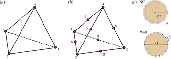
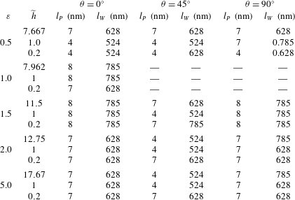
The 4-node and 10-node tetrahedrons used in the finite element representation of the computational domain are shown in panels (a) and (b), respectively. The top panel in (c) shows an icosahedron used in the discretization of a spherical particle of diameter
 $a$
which is later mapped to a spheroid – here
 $l_{P}$
denotes the mesh length on the particle surface. The lower panel in (c) shows the cross-section of a cylindrical tube of diameter
 $D$
. The mesh size on the particle surface is denoted by
 $l_{W}$
.

2.5 Spatial discretization
-
(i) Surface/boundary mesh: the boundaries of the computational domain are discretized as described in Hu et al. (Reference Hu, Patankar and Zhu2001). Briefly, as shown in figure 3(c), we start by approximating the surface of a unit sphere by an icosahedron and further subdivide the faces of the icosahedron into a triangular mesh with a predefined characteristic length
 $l_{P}$
. The triangular mesh on the icosahedron is stereographically projected to construct the boundary mesh for an spheroidal particle with specified values of
$a$
,
$b$
,
$c$
and
$\unicode[STIX]{x1D703}$
. Similarly, the cylindrical wall boundary is discretized into a triangular mesh with a characteristic length
$l_{W}$
. In the following, we will describe the finite element mesh parameters used in our calculations in terms of
$l_{P}$
and
$l_{W}$
.
-
(ii) Volume mesh: the fluid domain is discretized by tetrahedral finite elements generated using Delaunay–Voronoi methods. The discrete solution for the fluid velocity is approximated by piecewise quadratic functions and is assumed to be continuous over the domain. We use 10 node tetrahedral elements (figure 3 b) to locally interpolate the velocity. On the other hand, the pressure and the stress are piecewise linear and continuous, and are interpolated using 4-node tetrahedral elements (figure 3 a). The 4-node and 10-node elements used to interpolate the stress and the velocity are known to satisfy the Ladyzhenskaya–Babuska–Brezzi conditions for stability (Hu et al. Reference Hu, Patankar and Zhu2001).


For a given finite element mesh, the combined fluid–solid weak formulation (2.37) reduces to a nonlinear system of algebraic equations, which is solved by a Newton–Raphson algorithm. Similarly, the mesh velocity (2.25) and mesh acceleration (2.28) can also be reduced to linear systems of algebraic equations. These coupled systems are solved by a multigrid preconditioned conjugate gradient method.
2.6 Random stress tensor for the tetrahedral finite element mesh
We now describe the procedure to numerically generate the random stresses associated with the unstructured tetrahedral mesh. The random stress at each node on the computational domain depends on the volumes of the tetrahedrons associated with it.
The components of the random stress tensor
 $\unicode[STIX]{x1D64E}^{(i)}$
in the
 $i$
th tetrahedral element, with volume
 $V_{e}^{(i)}$
, is approximated from (2.5) as
 $$\begin{eqnarray}\displaystyle & \displaystyle \langle \unicode[STIX]{x1D61A}_{xx}\rangle ^{(i)}=\langle \unicode[STIX]{x1D61A}_{yy}\rangle ^{(i)}=\langle \unicode[STIX]{x1D61A}_{zz}\rangle ^{(i)}=0, & \displaystyle\end{eqnarray}$$
 $$\begin{eqnarray}\displaystyle & \displaystyle \langle \unicode[STIX]{x1D61A}_{xy}\rangle ^{(i)}=\langle \unicode[STIX]{x1D61A}_{yz}\rangle ^{(i)}=\langle \unicode[STIX]{x1D61A}_{zx}\rangle ^{(i)}=0, & \displaystyle\end{eqnarray}$$
 $$\begin{eqnarray}\displaystyle & \displaystyle \langle \unicode[STIX]{x1D61A}_{xx}^{2}\rangle ^{(i)}=\langle \unicode[STIX]{x1D61A}_{yy}^{2}\rangle ^{(i)}=\langle \unicode[STIX]{x1D61A}_{zz}^{2}\rangle ^{(i)}=\frac{4k_{B}T\unicode[STIX]{x1D707}}{V_{e}^{(i)}\unicode[STIX]{x0394}t}, & \displaystyle\end{eqnarray}$$
 $$\begin{eqnarray}\displaystyle & \displaystyle \langle \unicode[STIX]{x1D61A}_{xy}^{2}\rangle ^{(i)}=\langle \unicode[STIX]{x1D61A}_{yz}^{2}\rangle ^{(i)}=\langle \unicode[STIX]{x1D61A}_{zx}^{2}\rangle ^{(i)}=\frac{2k_{B}T\unicode[STIX]{x1D707}}{V_{e}^{(i)}\unicode[STIX]{x0394}t}, & \displaystyle\end{eqnarray}$$
where
 $\unicode[STIX]{x0394}t$
is the time step for the numerical simulation. The total stress on a node is then computed as:
 $$\begin{eqnarray}\displaystyle \unicode[STIX]{x1D64E}={\mathcal{C}}\mathop{\sum }_{i=1}^{N_{e}}\unicode[STIX]{x1D64E}^{(i)}, & & \displaystyle\end{eqnarray}$$
with
 ${\mathcal{C}}=1$
when the node is inside the computational domain and
 ${\mathcal{C}}=\sqrt{2}$
when the node is on a boundary surface.
 $N_{e}$
is the number of tetrahedrons associated with this node. At a boundary node, since we consider the spheroidal particles to be solid, the tetrahedral volume
 $V_{e}^{(i)}$
underestimates the total volume defined by the Dirac delta function
 $\unicode[STIX]{x1D6FF}(\boldsymbol{x}-\boldsymbol{x}^{\prime })$
, given in the right-hand side of (2.5). Ignoring the effect of the particle curvature on the estimate for
 $V_{e}^{(i)}$
, we approximate the effective volume as
 $\unicode[STIX]{x1D6FF}(\boldsymbol{x}-\boldsymbol{x}^{\prime })=2/V_{e}^{(i)}$
. Using this estimate in (2.41) and (2.42) and summing over all tetrahedral elements linked to a given node leads to the general equation given in (2.43).
2.7 Deterministic calculations to compute velocity autocorrelations in a quiescent fluid
In this study, we also employ a computationally inexpensive calculation to study the velocity autocorrelation function (VACF) and angular velocity autocorrelation function (AVACF) of a nano-spheroid. This method follows from the fluctuation–dissipation relation which states that the temporal correlation in the thermal stresses is equivalent to the correlation in the hydrodynamic memory of a stationary fluid (Kubo Reference Kubo1966). Earlier works (Pagonabarraga et al. Reference Pagonabarraga, Hagen, Lowe and Frenkel1998; Iwashita, Nakayama & Yamamoto Reference Iwashita, Nakayama and Yamamoto2008; Yu et al. Reference Yu, Eckmann, Ayyaswamy and Radhakrishnan2015) have shown that the averaged time correlation in the velocity of a Brownian particle, in a stationary medium, is equivalent to that for a driven particle computed in the absence of thermal fluctuations. This technique is called the deterministic method (Vitoshkin et al. Reference Vitoshkin, Yu, Eckmann, Ayyaswamy and Radhakrishnan2016).
Sincethe inclusionof the stochastic stresses (
 $\unicode[STIX]{x1D64E}\neq 0$
)in the fluctuatinghydrodynamics formulation leads to a large computational overhead, we may use the deterministic method to investigate the long-time behaviour of the velocity autocorrelation of the nano-spheroid in a quiescent medium. The formulation and numerical techniques for the deterministic method are similar to that for fluctuating hydrodynamics except that:
-
(i) the stochastic stress on each fluid element is taken to be
$\unicode[STIX]{x1D64E}=0$
, -
(ii) theinitialvalueoftheparticlevelocity (2.11)istakentobe
$\boldsymbol{U}(0)=(U_{x,0},U_{y,0},U_{z,0})$
and
$\unicode[STIX]{x1D734}(0)=(\unicode[STIX]{x1D6FA}_{x,0},\unicode[STIX]{x1D6FA}_{y,0},\unicode[STIX]{x1D6FA}_{z,0})$
with at least one of the components being non-zero.



It should be noted that, though the deterministic method provides an inexpensive route to compute the long-time correlations in the particle velocities, the trajectories obtained in these simulations are not reflective of those for a fluctuating particle.
2.8 Added masses and moments of inertia as functions of the aspect ratio
In our computational method we have employed an incompressible fluid formulation. To account for the corrections due to the incompressibility assumption, the effective masses and the moments of inertia must be included in our numerical evaluations, e.g. see Korotkin (Reference Korotkin2008), Uma et al. (Reference Uma, Swaminathan, Radhakrishnan, Eckmann and Ayyaswamy2011). In this section we present the expressions for the effective masses and moments of inertia (Korotkin Reference Korotkin2008) of a spheroidal particle in terms of its aspect ratio
 $\unicode[STIX]{x1D700}$
. The expressions for the added masses and moments of inertia of a general ellipsoid may be found in Korotkin (Reference Korotkin2008).
We define the direction dependent added masses and moments of inertia as:
 $$\begin{eqnarray}\displaystyle & \displaystyle m_{\unicode[STIX]{x1D6FC}}^{\ast }=(1+k_{\unicode[STIX]{x1D6FC}})m, & \displaystyle\end{eqnarray}$$
 $$\begin{eqnarray}\displaystyle & \displaystyle I_{\unicode[STIX]{x1D6FC}\unicode[STIX]{x1D6FC}}^{\ast }=(1+K_{\unicode[STIX]{x1D6FC}\unicode[STIX]{x1D6FC}})I_{\unicode[STIX]{x1D6FC}\unicode[STIX]{x1D6FC}}. & \displaystyle\end{eqnarray}$$
Here
 $k_{\unicode[STIX]{x1D6FC}}$
(
 $\unicode[STIX]{x1D6FC}=x$
,
 $y$
,
 $z$
) denotes the coefficient of the added mass along the
 $\unicode[STIX]{x1D6FC}$
direction, and
 $K_{\unicode[STIX]{x1D6FC}\unicode[STIX]{x1D6FC}}$
(
 $\unicode[STIX]{x1D6FC}=1$
,
 $2$
,
 $3$
) denotes the coefficient of the added moment of inertia along the principal direction
 $\unicode[STIX]{x1D6FC}$
. The analytical forms for the aspect ratio dependent values of
 $m_{\unicode[STIX]{x1D6FC}}^{\ast }$
and
 $I_{\unicode[STIX]{x1D6FC}\unicode[STIX]{x1D6FC}}^{\ast }$
for a spheroidal particle fully immersed in a fluid are as below:
2.8.1 Oblate spheroids (
$a<b=c$
and
$\unicode[STIX]{x1D700}<1.0$
)


For an oblate spheroid (with
 $a<b=c$
) and oriented such that the semi-minor axes is along the axial direction of the bounding wall, we define the coefficients:
 $$\begin{eqnarray}A_{ob}={\displaystyle \frac{2\unicode[STIX]{x1D700}}{(1-\unicode[STIX]{x1D700}^{2})^{3/2}}}\left({\displaystyle \frac{\sqrt{1-\unicode[STIX]{x1D700}^{2}}}{\unicode[STIX]{x1D700}}}-\sin ^{-1}\left(\sqrt{1-\unicode[STIX]{x1D700}^{2}}\right)\right),\end{eqnarray}$$
and
 $$\begin{eqnarray}B_{ob}=C_{ob}={\displaystyle \frac{\unicode[STIX]{x1D700}}{(1-\unicode[STIX]{x1D700}^{2})^{3/2}}}\left(\sin ^{-1}\left(\sqrt{1-\unicode[STIX]{x1D700}^{2}}\right)-\unicode[STIX]{x1D700}\sqrt{1-\unicode[STIX]{x1D700}^{2}}\right).\end{eqnarray}$$
The added mass coefficients may then be expressed in terms of
 $A_{ob}$
and
 $C_{ob}$
as:
 $$\begin{eqnarray}k_{x}={\displaystyle \frac{A_{ob}}{2C_{ob}}};\quad k_{y}=k_{z}={\displaystyle \frac{C_{ob}}{A_{ob}+C_{ob}}},\end{eqnarray}$$
 $$\begin{eqnarray}\displaystyle & \displaystyle K_{11}=0, & \displaystyle\end{eqnarray}$$
 $$\begin{eqnarray}\displaystyle & \displaystyle K_{22}=K_{33}={\displaystyle \frac{(1-\unicode[STIX]{x1D700}^{2})^{2}}{\unicode[STIX]{x1D700}^{2}+1}}\quad {\displaystyle \frac{A_{ob}-C_{ob}}{2(1-\unicode[STIX]{x1D700}^{2})+(C_{ob}-A_{ob})(\unicode[STIX]{x1D700}^{2}+1)}}. & \displaystyle\end{eqnarray}$$
2.8.2 Spherical particles (
$a=b=c$
and
$\unicode[STIX]{x1D700}=1.0$
)


For a spherical particle (2.48), (2.49) and (2.50) reduce to the well-known results for the added coefficients:
 $$\begin{eqnarray}k_{x}=k_{y}=k_{z}={\textstyle \frac{1}{2}},\end{eqnarray}$$
and
 $$\begin{eqnarray}K_{11}=K_{22}=K_{33}=0.\end{eqnarray}$$
2.8.3 Prolate spheroids (
$a>b=c$
and
$\unicode[STIX]{x1D700}>1.0$
)


For a prolate spheroid with its semi-major axes along the axial direction of the tube, we define the coefficients:
 $$\begin{eqnarray}\displaystyle & \displaystyle A_{pr}={\displaystyle \frac{2\unicode[STIX]{x1D700}}{(\unicode[STIX]{x1D700}^{2}-1)^{3/2}}}\left(\log \left(\sqrt{\unicode[STIX]{x1D700}^{2}-1}+\unicode[STIX]{x1D700}\right)-{\displaystyle \frac{\sqrt{\unicode[STIX]{x1D700}^{2}-1}}{\unicode[STIX]{x1D700}}}\right), & \displaystyle\end{eqnarray}$$
 $$\begin{eqnarray}\displaystyle & \displaystyle B_{pr}=C_{pr}={\displaystyle \frac{\unicode[STIX]{x1D700}^{2}}{\unicode[STIX]{x1D700}^{2}-1}}\left(1-{\displaystyle \frac{\sqrt{\unicode[STIX]{x1D700}^{2}-1}}{\unicode[STIX]{x1D700}}}\log \left(\sqrt{\unicode[STIX]{x1D700}^{2}-1}+\unicode[STIX]{x1D700}\right)\right). & \displaystyle\end{eqnarray}$$
The coefficients of the added masses and moments of inertia may then be expressed in terms of
 $A_{pr}$
and
 $C_{pr}$
as:
 $$\begin{eqnarray}k_{x}={\displaystyle \frac{A_{pr}}{2-A_{pr}}};\quad k_{y}=k_{z}={\displaystyle \frac{C_{pr}}{2-C_{pr}}},\end{eqnarray}$$
 $$\begin{eqnarray}\displaystyle & \displaystyle K_{11}=0, & \displaystyle\end{eqnarray}$$
 $$\begin{eqnarray}\displaystyle & \displaystyle K_{22}=K_{33}={\displaystyle \frac{(1-\unicode[STIX]{x1D700}^{2})^{2}}{1+\unicode[STIX]{x1D700}^{2}}}\quad {\displaystyle \frac{A_{pr}-C_{pr}}{2(1-\unicode[STIX]{x1D700}^{2})+(C_{pr}-A_{pr})(1+\unicode[STIX]{x1D700}^{2})}}. & \displaystyle\end{eqnarray}$$
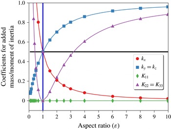
Equations (2.51) and (2.52) may be also be obtained as limiting cases of (2.55)–(2.57). The aspect ratio and direction dependent added masses and moments of inertia coefficients, given by (2.46)–(2.57), are shown in figure 4.
Coefficients of the added masses (
 $k_{x}$
,
 $k_{y}$
and
 $k_{z}$
) and moments of inertia (
 $K_{11}$
,
 $K_{22}$
and
 $K_{33}$
) as functions of
 $\unicode[STIX]{x1D700}$
, the aspect ratio of the particle. The horizontal line represents the added mass component for a spherical particle (
 $\unicode[STIX]{x1D700}=1$
), for which
 $k_{x}=k_{y}=k_{z}=0.5$
.

3 Numerical results and discussion
We study the motion of the particle in (i) a quiescent fluid medium, and (ii) a fully developed Poiseuille flow at the entrance. For particle motion in the presence of a Poiseuille flow, we initially fix the particle at the desired location and subsequently release it only when the flow is fully developed (Uma et al.
Reference Uma, Swaminathan, Radhakrishnan, Eckmann and Ayyaswamy2011). For the results reported in this study, we take the tube diameter
 $D$
to be in the range
 $5{-}50~\unicode[STIX]{x03BC}\text{m}$
and tube length
 $L=40~\unicode[STIX]{x03BC}\text{m}$
throughout. The dynamic viscosity and density of the fluid are taken to be
 $\unicode[STIX]{x1D707}=10^{-3}~\text{kg}~\text{m}^{-1}~\text{s}^{-1}$
, and
 $\unicode[STIX]{x1D70C}^{(f)}=10^{3}~\text{kg}~\text{m}^{-3}$
, respectively.
The presence of stochastic stresses (
 $\unicode[STIX]{x1D64E}\neq 0$
) continuously alters the degrees of freedom in the fluid and as a result the spheroidal particle is subject to a net force which has contributions from both the hydrodynamic and the stochastic stresses. First, we consider a stationary medium. In the absence of an external flow, the motion of the nanoparticle is solely Brownian.
The fluid temperature is set at
 $T=310~\text{K}$
and the thermal energy is given by
 $k_{B}T$
, with the Boltzmann constant
 $k_{B}=1.3806503\times 10^{-23}~\text{kg}~\text{m}^{2}~(\text{s}^{-2}~\text{K}^{-1})$
. We first consider a neutrally buoyant spheroidal NC of aspect ratio
 $\unicode[STIX]{x1D700}=1.5$
(with
 $a=600~\text{nm}$
and
 $b=c=400~\text{nm}$
and
 $\unicode[STIX]{x1D703}=0^{\circ }$
) initially placed at the centre of a fluid filled cylinder with
 $D=5~\unicode[STIX]{x03BC}\text{m}$
and
 $L=40~\unicode[STIX]{x03BC}\text{m}$
. The characteristic length of the particle is taken to be the equivalent spherical diameter
 $d_{eq}=\sqrt[3]{abc}=457.9~\text{nm}$
and this sets a representative hydrodynamic time scale
 $t_{\unicode[STIX]{x1D708}}=(d_{eq}/2)^{2}/\unicode[STIX]{x1D707}=5.24\times 10^{-8}$
s which will be employed for the scaling throughout the treatment. We have also examined the motion of this particle in the presence of a Poiseuille flow along the
 $x$
direction. In this case, flows with maximum inlet velocities in the range
 $u_{max}=10^{-1}$
–
 $10^{5}$
 $~\unicode[STIX]{x03BC}\text{m}~\text{s}^{-1}$
, corresponding to Péclet numbers (
 $Pe=d_{eq}u_{max}/D_{\infty }$
) in the range
 $2.31\times 10^{-2}$
–
 $2.31\times 10^{4}$
, and particle Reynolds numbers (
 $Re^{(p)}=\unicode[STIX]{x1D70C}^{(f)}d_{eq}u_{max}/\unicode[STIX]{x1D707}$
) in the range
 $5\times 10^{-8}$
–
 $5\times 10^{-2}$
, have been investigated. Here
 $D_{\infty }=2k_{B}T/(6\unicode[STIX]{x03C0}\unicode[STIX]{x1D707}d_{eq})$
is the Stokes–Einstein diffusivity for the equivalent spherical particle.
3.1 Thermal equilibration of the spheroidal NC
Since this study is a numerical evaluation of a stochastic differential equation formulation, it is very important to set formally correct procedures in place before embarking on the full evaluation. Rigorous requirements in this context consist of guaranteeing thermal equilibration of the NC with the bulk medium and the satisfaction of the Maxwell–Boltzmann distribution for the components of the particle velocity.
As stated earlier, the preset bulk fluid temperature is
 $T=310~\text{K}$
. We note that the fluid–particle system is a self-thermostat that maintains the equilibrium temperature through the fluctuation–dissipation relation. Using the equipartition theorem, we numerically estimate the translational and rotational temperatures, denoted by
 $T^{(t)}$
and
 $T^{(r)}$
respectively, as:
 $$\begin{eqnarray}\displaystyle T^{(t)}={\displaystyle \frac{T_{x}^{(t)}+T_{y}^{(t)}+T_{z}^{(t)}}{3}}=\frac{1}{3k_{B}}\mathop{\sum }_{\unicode[STIX]{x1D6FC}=x,y,z}m_{\unicode[STIX]{x1D6FC}}^{\ast }\langle U_{\unicode[STIX]{x1D6FC}}^{2}\rangle , & & \displaystyle\end{eqnarray}$$
and
 $$\begin{eqnarray}\displaystyle T^{(r)}={\displaystyle \frac{T_{1}^{(r)}+T_{2}^{(r)}+T_{3}^{(r)}}{3}}=\frac{1}{3k_{B}}\mathop{\sum }_{\unicode[STIX]{x1D6FC}=1,2,3}I_{\unicode[STIX]{x1D6FC}\unicode[STIX]{x1D6FC}}^{\ast }\langle \unicode[STIX]{x1D6FA}_{\unicode[STIX]{x1D6FC}}^{2}\rangle . & & \displaystyle\end{eqnarray}$$
In estimating these temperatures, we explicitly account for the effective masses
 $m_{\unicode[STIX]{x1D6FC}}^{\ast }$
and moments of inertia
 $I_{\unicode[STIX]{x1D6FC}\unicode[STIX]{x1D6FC}}^{\ast }$
, whose exact forms are given in (2.45).
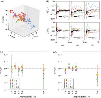
Figure 5(a) shows five independent trajectories of an NC, initially at the same starting location. The computations were carried out over a period of
 $3~\unicode[STIX]{x03BC}\text{s}$
using a time step of
 $\unicode[STIX]{x0394}t=10^{-10}~\text{s}$
. These trajectories demonstrate the Brownian characteristic of the particle. For each of these trajectories, we compute
 $T_{\unicode[STIX]{x1D6FC}}^{(t)}$
and
 $T_{\unicode[STIX]{x1D6FC}}^{(r)}$
, the translational and rotational temperatures, respectively, along each principal direction
 $\unicode[STIX]{x1D6FC}$
. The time evolution of
 $T_{\unicode[STIX]{x1D6FC}}^{(t)}$
and
 $T_{\unicode[STIX]{x1D6FC}}^{(r)}$
are shown in figure 5(b). Both the translational and rotational temperatures of the particle transition to a steady state at very short times (
 ${\sim}500\unicode[STIX]{x0394}t\simeq t_{\unicode[STIX]{x1D708}}$
) following their introduction into the fluid. While the temperatures of the individual trajectories fluctuate by as much as
 $\pm 15\,\%$
, the time-averaged temperatures, also shown alongside in each of the panels in figure 5(b), show thermal equilibration with the preset bulk temperature.
Next, we investigate the effect of various spheroidal NC aspect ratios on thermal equilibration. We consider five different aspect ratios,
 $\unicode[STIX]{x1D700}=0.5,1.0,1.5,2.0$
and 5.0 for which the translational and rotational temperatures are displayed in figure 5(c,d) – the complete set of data can be found in figures S1.1–S1.15 in the supplementary material available at https://doi.org/10.1017/jfm.2017.182. The NCs here all have an equivalent volume of
 $0.0502~~\unicode[STIX]{x03BC}\text{m}^{3}$
, which corresponds to an effective spherical diameter of
 $d_{eq}=457.9~\text{nm}$
, as before. In this context, we have also studied the effect of confinement on the thermodynamic behaviour of the NCs by computing their equilibrations for three wall separation distances, chosen such that the NC is in (i) the bulk regime (
 $\widetilde{h}>1$
), (ii) the near wall regime (
 $\widetilde{h}=1$
) and (iii) the lubrication regime (
 $\widetilde{h}=0.2$
). We note that
 $\widetilde{h}$
is the non-dimensional particle separation from the curved wall and is a function of
 $\unicode[STIX]{x1D700}$
and the particle orientation (see appendix B). The computed values of
 $T^{(t)}$
and
 $T^{(r)}$
are averaged over 10 independent
 $3~\unicode[STIX]{x03BC}\text{s}$
trajectories, and these are shown in figure 5(c,d), respectively. The evaluated particle temperatures match with that of the bulk fluid within
 $\pm 15\,\%$
, independent of the aspect ratios and confinement effects. The larger deviations seen for
 $\unicode[STIX]{x1D700}=5.0$
may further be improved by refining the computational mesh, which we discuss next.
(a) Five independent trajectories of a spheroidal particle (with
 $\unicode[STIX]{x1D700}=1.5$
and
 $a=600~\text{nm}$
) immersed in a fluid with fluctuating stresses. (b) Time evolution of the scaled translational and rotational temperatures, along the
 $x$
,
 $y$
and
 $z$
directions, for all the five trajectories, along with their ensemble-averaged value. (c,d) Translational and rotational temperatures, averaged over all directions, as a function of
 $\unicode[STIX]{x1D700}$
, the aspect ratio of the spheroidal NC, for three different positions with respect to the bounding wall. Mesh parameters used are
 $l_{P}=6~\text{nm}$
and
 $l_{W}=785~\text{nm}$
. The exact values for
 $\widetilde{h}>1$
for different
 $\unicode[STIX]{x1D716}$
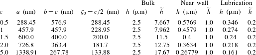
may be found in table 1.

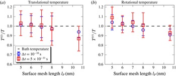
The computed values of the equilibrium temperature depend both on the resolution of the computational mesh (i.e. on
 $l_{P}$
and
 $l_{W}$
in figure 3(c)) and the time step
 $\unicode[STIX]{x0394}t$
. This is illustrated in figure 6, for an NC with
 $\unicode[STIX]{x1D700}=1.5$
,
 $a=600~\text{nm}$
, and
 $\unicode[STIX]{x1D703}=0^{\circ }$
, where we show
 $T^{(t)}$
and
 $T^{(r)}$
as functions of
 $l_{P}$
computed for two time steps
 $\unicode[STIX]{x0394}t=10^{-10}$
s and
 $\unicode[STIX]{x0394}t=5\times 10^{-11}$
s. The error bars correspond to the standard deviation in the temperatures computed from 10 independent ensembles and the maximum error in the predictions is found to be around
 $15\,\%$
. For the condition of the study, for
 $l_{P}\sim 8~\text{nm}$
the estimates of the equilibrated temperatures are almost the same as the bath temperature
 $T$
confirming equilibration. Beyond
 $l_{P}=8~\text{nm}$
, equilibrium is not attained because of the inability to determine the stress and the corresponding velocity fields sufficiently accurately. It is important therefore to correctly estimate the mesh length that yields equilibration for the prevailing conditions. These studies establish the criteria for mesh convergence in stochastic hydrodynamic computations.
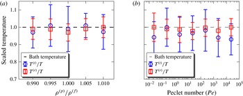
Figure 7(a) shows
 $T^{(t)}$
and
 $T^{(r)}$
for a nearly neutrally buoyant spheroidal particle, of similar dimensions as before, for five different particle densities that are chosen to be in the range
 $990\leqslant \unicode[STIX]{x1D70C}^{(p)}\leqslant 1010~\text{kg}~\text{m}^{-3}$
, in thermal equilibrium with a quiescent fluid. We find for the range of densities investigated that thermal equilibration is attained in a manner similar to that described earlier.
We next study how the presence of external flow impacts the stochastic motion of the NC by introducing it at the centre of a tube with a well-developed incoming Poiseuille flow. We investigate this phenomenon for seven different flow rates with the NC Péclet numbers in the range
 $Pe=2.31\times 10^{-2}$
–
 $2.31\times 10^{4}$
. Figure 7(b) shows the translational and rotational temperatures as a function of
 $Pe$
for a neutrally buoyant spheroidal NC with a normalized surface mesh length of
 $l_{P}=5~\text{nm}$
and
 $l_{W}=785~\text{nm}$
. Our results show that equilibration is attained by the NC in a manner similar to the above even in the presence of weak Poiseuille flows.
Translational and rotational temperatures of the NC as a function of the surface mesh length, for two values of the computational time step:
 $\unicode[STIX]{x0394}t=10^{-10}~\text{s}$
and
 $\unicode[STIX]{x0394}t=5\times 10-11~\text{s}$
.

Translational and rotational temperatures of the spheroidal nanocarrier (a) as a function of
 $\unicode[STIX]{x1D70C}^{(p)}/\unicode[STIX]{x1D70C}^{(f)}$
in a stationary fluid medium, and (b) as a function of the Péclet number (
 $Pe$
) in a Poiseuille flow with
 $\unicode[STIX]{x1D70C}^{(p)}/\unicode[STIX]{x1D70C}^{(f)}=1$
. Mesh parameters used are
 $l_{P}=6~\text{nm}$
and
 $l_{W}=785~\text{nm}$
.

Having shown that the spheroidal NC satisfies the principle of equipartition of translational and rotational energies, we next investigate the behaviour of the velocity components.
To be self-consistent, in this section we show that the translational and rotational velocities of the NC in the fluctuating fluid satisfy:
 $$\begin{eqnarray}P(U_{\unicode[STIX]{x1D6FC}})\,\text{d}U_{\unicode[STIX]{x1D6FC}}={\displaystyle \frac{1}{\sqrt{2\unicode[STIX]{x03C0}}}}\exp \left(-{\displaystyle \frac{U_{\unicode[STIX]{x1D6FC}}^{2}}{2\unicode[STIX]{x1D70E}_{(t),\unicode[STIX]{x1D6FC}}^{2}}}\right),\end{eqnarray}$$
and
 $$\begin{eqnarray}P(\unicode[STIX]{x1D6FA}_{\unicode[STIX]{x1D6FC}})\,\text{d}\unicode[STIX]{x1D6FA}_{\unicode[STIX]{x1D6FC}}={\displaystyle \frac{1}{\sqrt{2\unicode[STIX]{x03C0}}}}\exp \left(-{\displaystyle \frac{\unicode[STIX]{x1D6FA}_{\unicode[STIX]{x1D6FC}}^{2}}{2\unicode[STIX]{x1D70E}_{(r),\unicode[STIX]{x1D6FC}}^{2}}}\right),\end{eqnarray}$$
respectively. Here
 $\unicode[STIX]{x1D70E}_{(t),\unicode[STIX]{x1D6FC}}^{2}=k_{B}T/m_{\unicode[STIX]{x1D6FC}}^{\ast }$
is the variance in the
 $\unicode[STIX]{x1D6FC}$
component of the particle translational velocity, with
 $\unicode[STIX]{x1D6FC}=x,y,z$
and
 $\unicode[STIX]{x1D70E}_{(r),\unicode[STIX]{x1D6FC}}^{2}=k_{B}T/I_{\unicode[STIX]{x1D6FC}\unicode[STIX]{x1D6FC}}^{\ast }$
, with
 $\unicode[STIX]{x1D6FC}=1,2,3$
the variance in the rotational velocities.
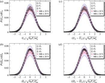
The corresponding probability distributions for a spheroidal particle, with
 $\unicode[STIX]{x1D700}=1.5$
,
 $a=600~\text{nm}$
and
 $\unicode[STIX]{x1D703}=0^{\circ }$
, placed at the centre of the tube, is shown in figure 8(a,b).
 $P(U_{\unicode[STIX]{x1D6FC}})\,\text{d}U_{\unicode[STIX]{x1D6FC}}$
shows a normal distribution, for all values of
 $\unicode[STIX]{x1D6FC}=x$
,
 $y$
and
 $z$
. Furthermore, the computed probabilities deviate at most by 10 % from the normal distribution as is shown by the shaded region that represents a
 $\pm 10\,\%$
deviation. We also studied the velocity distribution for a spheroidal NC placed at the centre of a tube with a steady Poiseuille flow with
 $u_{max}=100~~\unicode[STIX]{x03BC}\text{m}~\text{s}^{-1}$
.
 $P(U_{\unicode[STIX]{x1D6FC}})\,\text{d}U_{\unicode[STIX]{x1D6FC}}$
in the presence of flow is shown in figure 8(c,d), and both the translational and rotational velocities show a normal distribution consistent with Maxwell–Boltzmann statistics.
Equilibrium probability of the translational and rotational velocities of a spheroidal nanoparticle in a quiescent fluid (a,b) and in a Poiseuille flow (c,d). The two shaded regions in each of the panels represent deviations of
 $\pm 10\,\%$
and
 $\pm 20\,\%$
from the Maxwell–Boltzmann (MB) distribution. Data shown for an NC with
 $\unicode[STIX]{x1D700}=1.5$
,
 $a=600~\text{nm}$
, and
 $\unicode[STIX]{x1D703}=0^{\circ }$
placed at the centre of a cylindrical tube of diameter
 $D=5~\unicode[STIX]{x03BC}\text{m}$
. Mesh parameters used are
 $l_{P}=7~\text{nm}$
and
 $l_{W}=785~\text{nm}$
.

3.2 Translational velocity autocorrelation and rotational velocity autocorrelation of the spheroidal NC
We define the VACF of the NC velocities as
 $$\begin{eqnarray}C_{U_{\unicode[STIX]{x1D6FC}}}(t)=\frac{\left\langle U_{\unicode[STIX]{x1D6FC}}(0)U_{\unicode[STIX]{x1D6FC}}(t)\right\rangle }{(k_{B}T/m_{\unicode[STIX]{x1D6FC}}^{\ast })}\quad \forall \unicode[STIX]{x1D6FC}=x,y,z\end{eqnarray}$$
and the AVACF as
 $$\begin{eqnarray}C_{\unicode[STIX]{x1D6FA}_{\unicode[STIX]{x1D6FC}}}(t)=\frac{\left\langle \unicode[STIX]{x1D6FA}_{\unicode[STIX]{x1D6FC}}(0)\unicode[STIX]{x1D6FA}_{\unicode[STIX]{x1D6FC}}(t)\right\rangle }{(k_{B}T/I_{\unicode[STIX]{x1D6FC}\unicode[STIX]{x1D6FC}}^{\ast })}\quad \forall \unicode[STIX]{x1D6FC}=1,2,3.\end{eqnarray}$$
We compute the VACF and AVACF of a Brownian NC using two methods: (i) direct calculations using the fluctuating hydrodynamics approach and (ii) from the relaxation of the velocity using the deterministic method. It has been previously shown that for a sufficiently small initial velocity, the decay of the NC velocity is identical to the velocity autocorrelation function, and in scaled units, we express the VACF and AVACF from the deterministic method as:
 $$\begin{eqnarray}C_{U_{\unicode[STIX]{x1D6FC}}}(t)=\frac{U_{\unicode[STIX]{x1D6FC}}(t)}{U_{\unicode[STIX]{x1D6FC}}(0)}\quad \forall \unicode[STIX]{x1D6FC}=x,y,z,\end{eqnarray}$$
and
 $$\begin{eqnarray}C_{\unicode[STIX]{x1D6FA}_{\unicode[STIX]{x1D6FC}}}(t)=\frac{\unicode[STIX]{x1D6FA}_{\unicode[STIX]{x1D6FC}}(t)}{\unicode[STIX]{x1D6FA}_{\unicode[STIX]{x1D6FC}}(0)}\quad \forall \unicode[STIX]{x1D6FC}=1,2,3.\end{eqnarray}$$
The time correlation in the translational and rotational velocities of a Brownian particle in the absence of hydrodynamic interactions decays as:
 $$\begin{eqnarray}C_{U_{\unicode[STIX]{x1D6FC}}}(t)=\exp \left(-\frac{t}{{\mathcal{M}}_{\unicode[STIX]{x1D6FC}}^{(t)}m_{\unicode[STIX]{x1D6FC}}^{\ast }}\right),\end{eqnarray}$$
and
 $$\begin{eqnarray}C_{\unicode[STIX]{x1D6FA}_{\unicode[STIX]{x1D6FC}}}(t)=\exp \left(-\frac{t}{{\mathcal{M}}_{\unicode[STIX]{x1D6FC}}^{(r)}I_{\unicode[STIX]{x1D6FC}\unicode[STIX]{x1D6FC}}^{\ast }}\right),\end{eqnarray}$$
respectively. Here, we denote the translational and rotational mobilities of the particle, along the
 $\unicode[STIX]{x1D6FC}$
direction, as
 ${\mathcal{M}}_{\unicode[STIX]{x1D6FC}}^{(t)}$
and
 ${\mathcal{M}}_{\unicode[STIX]{x1D6FC}}^{(r)}$
, respectively. (The mobilities are estimated from the towing method described in § S3 in the supplementary material. In all of our results presented for the VACF we use mobilities computed using this method to show the duration of the first exponential decay regime.) However, when the hydrodynamic forces are explicitly taken into account, the exponential decay only holds for times smaller than the viscous relaxation time
 $t_{\unicode[STIX]{x1D708}}$
(i.e. for
 $t\leqslant t_{\unicode[STIX]{x1D708}}$
). The long-time behaviour (
 $t>t_{\unicode[STIX]{x1D708}}$
) of the VACF and AVACF for a spheroidal particle immersed in a bulk fluid follows an algebraic decay (Hocquart & Hinch Reference Hocquart and Hinch1983; Cichocki & Felderhof Reference Cichocki and Felderhof1995; Lowe, Frenkel & Masters Reference Lowe, Frenkel and Masters1995; Cichocki & Felderhof Reference Cichocki and Felderhof1996; Masters Reference Masters1996; Cichocki & Felderhof Reference Cichocki and Felderhof1997; Masters Reference Masters1997) given by
 $$\begin{eqnarray}C_{U_{\unicode[STIX]{x1D6FC}}}(t)=\frac{1}{6\sqrt{\unicode[STIX]{x03C0}}}\left(\frac{t}{t_{\unicode[STIX]{x1D708}}}\right)^{-3/2}\quad \text{for translational velocities }(\unicode[STIX]{x1D6FC}=x,y,z),\end{eqnarray}$$
and
 $$\begin{eqnarray}C_{\unicode[STIX]{x1D6FA}_{\unicode[STIX]{x1D6FC}}}(t)=\frac{\unicode[STIX]{x1D6F9}_{\unicode[STIX]{x1D6FC}\unicode[STIX]{x1D6FC}}^{A}}{60\sqrt{\unicode[STIX]{x03C0}}}\left(\frac{t}{t_{\unicode[STIX]{x1D708}}}\right)^{-5/2}\quad \text{for rotational velocities }(\unicode[STIX]{x1D6FC}=1,2,3).\end{eqnarray}$$
Here
 $$\begin{eqnarray}\unicode[STIX]{x1D6F9}_{\unicode[STIX]{x1D6FC}\unicode[STIX]{x1D6FC}}^{A}={\displaystyle \frac{I_{\unicode[STIX]{x1D6FC}\unicode[STIX]{x1D6FC}}^{\ast }}{I_{sph}}}\left(1+{\displaystyle \frac{3}{5}}\left({\displaystyle \frac{\unicode[STIX]{x1D716}_{\unicode[STIX]{x1D6FD}\unicode[STIX]{x1D6FE}}^{2}-1}{\unicode[STIX]{x1D716}_{\unicode[STIX]{x1D6FD}\unicode[STIX]{x1D6FE}}^{2}+1}}\right)^{2}\right).\end{eqnarray}$$
 $I_{\unicode[STIX]{x1D6FC}\unicode[STIX]{x1D6FC}}^{\ast }$
is the added moment of inertia along the
 $\unicode[STIX]{x1D6FC}$
direction and
 $I_{sph}$
is the moment of inertia of the equivalent sphere. The indices
 $\unicode[STIX]{x1D6FC},\unicode[STIX]{x1D6FD},\unicode[STIX]{x1D6FE}$
form a cyclic pair, such that
 $\unicode[STIX]{x1D6FD}=2$
and
 $\unicode[STIX]{x1D6FE}=3$
when
 $\unicode[STIX]{x1D6FC}=1$
, and
 $\unicode[STIX]{x1D716}_{\unicode[STIX]{x1D6FD}\unicode[STIX]{x1D6FE}}$
is the ratio of the particle dimensions along the
 $\unicode[STIX]{x1D6FD}$
and
 $\unicode[STIX]{x1D6FE}$
directions. For example, for a prolate spheroid (with
 $\unicode[STIX]{x1D700}=1.5$
)
 $\unicode[STIX]{x1D716}_{23}=1$
,
 $\unicode[STIX]{x1D716}_{31}=2/3$
and
 $\unicode[STIX]{x1D716}_{12}=3/2$
.
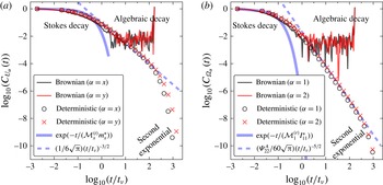
In figure 9 we show the VACF and AVACF for a spheroidal NC, with
 $\unicode[STIX]{x1D700}=1.5$
,
 $a=600~\text{nm}$
and
 $\unicode[STIX]{x1D703}=0^{\circ }$
, placed at the centre of the tube with
 $D=5~\unicode[STIX]{x03BC}\text{m}$
and
 $L=40~\unicode[STIX]{x03BC}\text{m}$
, for which
 $\widetilde{h}=11.5$
. In both panels, the solid lines correspond to data obtained from stochastic simulations and the symbols denote those obtained from the deterministic method. All data for the stochastic simulations have been averaged over 10 independent
 $3~\unicode[STIX]{x03BC}\text{s}$
Brownian trajectories.
(a)
 $C_{U_{\unicode[STIX]{x1D6FC}}}(t)$
, the VACF for
 $\unicode[STIX]{x1D6FC}=x,y$
and (b)
 $C_{\unicode[STIX]{x1D6FA}_{\unicode[STIX]{x1D6FC}}}(t)$
, the AVACF for
 $\unicode[STIX]{x1D6FC}=1,2$
, for a spheroidal NC (
 $\unicode[STIX]{x1D700}=1.5$
and
 $a=600~\text{nm}$
) placed at the centre of a cylindrical tube, with
 $\unicode[STIX]{x1D703}=0^{\circ }$
and
 $\widetilde{h}=11.5$
. In both the panels the solid lines correspond to data obtained from stochastic simulations and the symbols denote those obtained using the deterministic method. The correlations in the particle velocity show a Stokes exponential decay for
 $t<t_{\unicode[STIX]{x1D708}}$
and an algebraic decay for
 $t>t_{\unicode[STIX]{x1D708}}$
.

The VACF and AVACF shown in figure 9(a,b) show an initial Stokes exponential decay for
 $t<t_{\unicode[STIX]{x1D708}}$
followed by an algebraic decay for
 $t>t_{\unicode[STIX]{x1D708}}$
culminating in a second exponential decay for large times. For
 $t<t_{\unicode[STIX]{x1D708}}$
, the estimates from both the stochastic and deterministic methods agree very well with each other. The observed exponential decay agrees favourably with that predicted for this regime by (3.9) and (3.10). When
 $t>t_{\unicode[STIX]{x1D708}}$
, the VACF and AVACF from the deterministic method shows a cross-over to a power-law behaviour. The behaviour for the VACF scales as
 $(t/t_{\unicode[STIX]{x1D708}})^{-3/2}/(6\sqrt{\unicode[STIX]{x03C0}})$
for all the coordinate directions
 $x$
,
 $y$
and
 $z$
. For the AVACF, the scaling law is given by
 $\unicode[STIX]{x1D6F9}_{11}^{A}(t/t_{\unicode[STIX]{x1D708}})^{-5/2}/(60\sqrt{\unicode[STIX]{x03C0}})$
, with
 $\unicode[STIX]{x1D6F9}_{11}^{A}=I_{11}^{\ast }/I_{sph}$
along the 1 direction and
 $\unicode[STIX]{x1D6F9}_{22}^{A}(t/t_{\unicode[STIX]{x1D708}})^{-5/2}/(60\sqrt{\unicode[STIX]{x03C0}})$
, with
 $\unicode[STIX]{x1D6F9}_{22}^{A}=1.089(I_{22}^{\ast }/I_{sph})$
along the 2 and 3 directions. These scaling laws have been displayed with dotted lines in figure 9(a,b). Significantly, these predictions compare very favourably with the theoretical estimates of Hocquart & Hinch (Reference Hocquart and Hinch1983), thus lending credibility to this numerical undertaking. For both VACF and AVACF, at large times a second exponential decay is observed. This behaviour is attributable to the presence of the curved boundary of the vessel wall and its interaction with the NC motions.
It is noteworthy that the predictions of the detailed numerical stochastic calculations and those of the deterministic method compare very well. The detailed stochastic calculations are very time consuming and computationally prohibitively expensive at large times. However, the deterministic calculations that yield essentially the same results have a lower computational overhead.
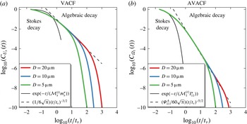
In figure 10(a,b) we display the translational and rotational VACFs, respectively, for a NC with
 $\unicode[STIX]{x1D700}=1.5$
,
 $a=600~\text{nm}$
and
 $\unicode[STIX]{x1D703}=0^{\circ }$
. The translational quantities are for the
 $x$
direction while that for rotation corresponds to the
 $1$
direction. Three different vessel confinements of diameters of
 $D=5,\,10$
and
 $20~\unicode[STIX]{x03BC}\text{m}$
with a fixed length of
 $L=40~\unicode[STIX]{x03BC}\text{m}$
are considered. In all of these cases, the particle is initially located on the central axis of the confining tube, with
 $\widetilde{h}=11.5$
,
 $24$
and
 $49$
, respectively. As noted in the figures three distinct decay regimes may be identified: an initial exponential decay, followed by an algebraic decay culminating in a second exponential decay. The first exponential decay regime lasts nearly the same time for all values of
 $D$
, as would be expected. Larger the
 $D$
the corresponding algebraic decay regime is of longer duration. The first exponential decay may be thought as being due to an uncorrelated noise, the algebraic decay is due to the combined effects of the thermal noise and hydrodynamic correlations while the second exponential decay shows the influence of momentum reflections from the confining boundary (Vitoshkin et al.
Reference Vitoshkin, Yu, Eckmann, Ayyaswamy and Radhakrishnan2016). The computed algebraic regimes agree very well with the analytical predictions given in (3.11) and (3.12) thus providing an important validation for the comprehensive numerical formulation undertaken in this study. The analytical predictions are displayed by dotted lines and as can be seen they overpredict both at short and long times. It is worthwhile emphasising that both the short and long time scales have been accessed in these numerical evaluations and this has been possible by the use of both the fluctuating hydrodynamics and the deterministic methods. The effects of confinements can only be accurately described by employing simulations as carried out in this paper.
Effect of wall confinement on the VACF (along the
 $x$
direction) and AVACF (along the 1 direction) computed using the deterministic method. Data shown for a NC with
 $\unicode[STIX]{x1D700}=1.5$
,
 $a=600~\text{nm}$
and
 $\unicode[STIX]{x1D703}=0^{\circ }$
placed at the centre of a cylindrical tube with
 $D=5,\,10$
and
 $20~\unicode[STIX]{x03BC}\text{m}$
. The solid and dotted lines denote the Stokes decay and algebraic decay regimes respectively.

There has been a considerable amount of published literature (Hocquart & Hinch Reference Hocquart and Hinch1983; Cichocki & Felderhof Reference Cichocki and Felderhof1995; Lowe et al.
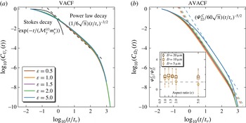
Reference Lowe, Frenkel and Masters1995; Cichocki & Felderhof Reference Cichocki and Felderhof1996; Masters Reference Masters1996; Cichocki & Felderhof Reference Cichocki and Felderhof1997; Masters Reference Masters1997) related to the particle shape dependence on the VACF and AVACF. Almost all of these studies concern themselves with the long-time algebraic decay of the AVACF in unconfined systems. Their results also state that the VACF in such circumstances is independent of the NC shape. We present numerically accurate values for the VACF and AVACF taking into account the effect of confinement. In this context, the effect of various aspect ratios,
 $\unicode[STIX]{x1D700}=0.5,\,1.0,\,1.5,\,2.0,$
and
 $5.0$
, on the translational and rotational VACFs along the
 $y$
and
 $2$
directions are displayed in figure 11(a,b) for an spheroidal NC that is placed at the centre of a cylindrical tube with
 $D=20~\unicode[STIX]{x03BC}\text{m}$
and
 $L=40~\unicode[STIX]{x03BC}\text{m}$
. The VACF (panel a) is found to be independent of the aspect ratio of the particle, with the algebraic regime scaling as
 $(t/t_{\unicode[STIX]{x1D708}})^{-3/2}/(6\sqrt{\unicode[STIX]{x03C0}})$
, which is shown as dotted lines. The AVACF (panel b), on the other hand, shows a strong dependence on the aspect ratio of the particle, particularly in the algebraic decay regime. This dependence has been captured by fitting this regime to
 $\unicode[STIX]{x1D6F9}_{22}^{C}(t/t_{\unicode[STIX]{x1D708}})^{-5/2}/(60\sqrt{\unicode[STIX]{x03C0}})$
, which is also shown alongside as dotted lines. In the inset, we compare the computed prefactor
 $\unicode[STIX]{x1D6F9}_{22}^{C}$
, for five different aspect ratios, to their corresponding analytical estimates given by
 $\unicode[STIX]{x1D6F9}_{22}^{A}$
, whose form is given in (3.13). Again excellent comparison with analytical predictions lend credibility to the numerical study. As discussed earlier, three distinct regimes may be identified: Stokes decay, algebraic decay followed by a second exponential decay which reflects the effect of confinement. It is to be noted that the scaling behaviour of both the VACF and AVACF may be modified from that given by (3.11) and (3.12) by changes in the NC–wall proximity and wall curvature. These aspects are displayed in § S2 of the supplementary material.
Effects of aspect ratios on the VACF and AVACF along the
 $y$
and
 $2$
directions, respectively. The main plot shows data for NCs confined by a tube with
 $D=20~\unicode[STIX]{x03BC}\text{m}$
. The dotted lines in panel (b) are the best fit curves for the algebraic decay regime which in turn is used to calculate
 $\unicode[STIX]{x1D6F9}_{22}^{C}(\unicode[STIX]{x1D700})$
. The inset to panel (b) shows a comparison of
 $\unicode[STIX]{x1D6F9}_{22}^{C}$
to their analytical estimates as a function of
 $\unicode[STIX]{x1D700}$
.

3.3 Diffusion of the spheroidal nanoparticle
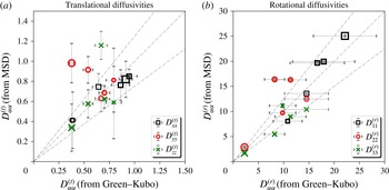
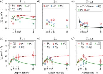
The evaluation of the various velocity autocorrelation functions enables the calculation of the particle diffusivities via the Green–Kubo relation (Kubo Reference Kubo1966). The diagonal components of the translational diffusion tensor
 $\unicode[STIX]{x1D63F}^{(t)}$
may be estimated from the VACF as:
 $$\begin{eqnarray}\unicode[STIX]{x1D60B}_{\unicode[STIX]{x1D6FC}\unicode[STIX]{x1D6FC}}^{(t)}(t)=\int _{0}^{t}\langle U_{\unicode[STIX]{x1D6FC}}(\unicode[STIX]{x1D70F})U_{\unicode[STIX]{x1D6FC}}(t+\unicode[STIX]{x1D70F})\rangle \,\text{d}\unicode[STIX]{x1D70F}\quad \forall \unicode[STIX]{x1D6FC}=x,y,\,\text{and }z.\end{eqnarray}$$
A similar expression also holds for the rotational diffusion tensor
 $\unicode[STIX]{x1D63F}^{(r)}$
, with
 $\unicode[STIX]{x1D6FC}=1$
, 2 and 3 (see Balakrishnan (Reference Balakrishnan2008) for details). Alternatively, the diffusive behaviour of the NC can also be ascertained from the scaling behaviour of the mean squared translational and rotational displacements defined by,
 $$\begin{eqnarray}\left\langle \unicode[STIX]{x0394}X_{\unicode[STIX]{x1D6FC}\unicode[STIX]{x1D6FC}}(t)\right\rangle =\left\langle \left(X_{\unicode[STIX]{x1D6FC}}(t+\unicode[STIX]{x1D70F})-X_{\unicode[STIX]{x1D6FC}}(\unicode[STIX]{x1D70F})\right)^{2}\right\rangle\end{eqnarray}$$
for the translational mean squared displacement (MSD), with
 $\unicode[STIX]{x1D6FC},\unicode[STIX]{x1D6FD}=x,y,z$
and
 $$\begin{eqnarray}\left\langle \unicode[STIX]{x0394}\unicode[STIX]{x1D6E9}_{\unicode[STIX]{x1D6FC}\unicode[STIX]{x1D6FC}}(t)\right\rangle =\left\langle \left(\unicode[STIX]{x1D6E9}_{\unicode[STIX]{x1D6FC}}(t+\unicode[STIX]{x1D70F})-\unicode[STIX]{x1D6E9}_{\unicode[STIX]{x1D6FC}}(\unicode[STIX]{x1D70F})\right)^{2}\right\rangle\end{eqnarray}$$
for the rotational MSD with
 $\unicode[STIX]{x1D6FC},\unicode[STIX]{x1D6FD}=1,2,3$
. For
 $t\gg t_{\unicode[STIX]{x1D708}}$
, the translational and rotational MSDs scale as:
 $$\begin{eqnarray}\lim _{t\rightarrow \infty }\langle \unicode[STIX]{x0394}X_{\unicode[STIX]{x1D6FC}\unicode[STIX]{x1D6FC}}(t)\rangle =2D_{\unicode[STIX]{x1D6FC}\unicode[STIX]{x1D6FC}}^{(t)}t\end{eqnarray}$$
and
 $$\begin{eqnarray}\lim _{t\rightarrow \infty }\left\langle \unicode[STIX]{x0394}\unicode[STIX]{x1D6E9}_{\unicode[STIX]{x1D6FC}\unicode[STIX]{x1D6FC}}(t)\right\rangle =2D_{\unicode[STIX]{x1D6FC}\unicode[STIX]{x1D6FC}}^{(r)}t,\end{eqnarray}$$
respectively.
A numerical evaluation of these equations will provide the zero-frequency diffusivity of the particle. It should also be noted that in systems with finite boundaries the linear scaling relations for the mean squared displacement may break down at large values of
 $t$
, due to the effects of confinement.
Mean squared displacement along various directions, for a neutrally buoyant spheroidal NC, with
 $\unicode[STIX]{x1D700}=1.5$
,
 $a=600~\text{nm}$
, and
 $\unicode[STIX]{x1D703}=0^{\circ }$
, placed at the centre of a stationary fluid medium. The translational MSD,
 $\unicode[STIX]{x0394}X_{\unicode[STIX]{x1D6FC}\unicode[STIX]{x1D6FC}}(t)$
for
 $\unicode[STIX]{x1D6FC}=x,y,z$
, and the rotational MSD,
 $\unicode[STIX]{x0394}\unicode[STIX]{x1D6E9}_{\unicode[STIX]{x1D6FC}\unicode[STIX]{x1D6FC}}(t)$
for
 $\unicode[STIX]{x1D6FC}=1,2,3$
, are shown in (a–f). The solid lines are the fits to the ballistic and diffusive regimes. Mesh parameters used are
 $l_{P}=7~\text{nm}$
and
 $l_{W}=785$
nm.

We first compute the diffusivity from the MSD calculations and compare them with estimates obtained using the Green–Kubo relation. Here, we numerically evaluate the MSD, along the various directions, for a neutrally buoyant spheroidal NC, with
 $\unicode[STIX]{x1D700}=1.5$
,
 $a=600~\text{nm}$
and
 $\unicode[STIX]{x1D703}=0^{\circ }$
, placed at the centre of a tube with
 $D=5~\unicode[STIX]{x03BC}\text{m}$
and
 $L=40~\unicode[STIX]{x03BC}\text{m}$
. The translational MSD,
 $\unicode[STIX]{x0394}X_{\unicode[STIX]{x1D6FC}\unicode[STIX]{x1D6FC}}(t)$
for
 $\unicode[STIX]{x1D6FC}=x,y,z$
, and the rotational MSD,
 $\unicode[STIX]{x0394}\unicode[STIX]{x1D6E9}_{\unicode[STIX]{x1D6FC}\unicode[STIX]{x1D6FC}}(t)$
for
 $\unicode[STIX]{x1D6FC}=1,2,3$
, are shown in figure 12(a–f). We observe that all the mean squared displacements cross-over from a ballistic regime (
 ${\sim}t^{2}$
) at short times to a diffusive regime (
 ${\sim}t$
) at longer times. For the NC investigated, this cross-over for the translational MSD is seen when
 $0.08t_{\unicode[STIX]{x1D708}}<t<5t_{\unicode[STIX]{x1D708}}$
and for the rotational MSD when
 $0.05t_{\unicode[STIX]{x1D708}}<t<t_{\unicode[STIX]{x1D708}}$
. We fit the ballistic regime to the functions
 $B_{\unicode[STIX]{x1D6FC}\unicode[STIX]{x1D6FC}}^{(t)}t^{2}$
(with
 $\unicode[STIX]{x1D6FC}=x,y$
and
 $z$
) and
 $B_{\unicode[STIX]{x1D6FC}\unicode[STIX]{x1D6FC}}^{(r)}t^{2}$
(with
 $\unicode[STIX]{x1D6FC}=1,2$
and
 $3$
), for the translational and rotational components, respectively, while the corresponding diffusive regimes are fit to (3.17) and (3.18). The best fits to each of these regimes are shown as solid lines. These enable the direct evaluation of NC diffusivities. Panels (a–f) reveal the important feature that the directional diffusivities are different for an spheroidal NC and vary along the directions
 $x$
,
 $y$
,
 $z$
and
 $1$
,
 $2$
,
 $3$
.
In figure 13, we compare the directional diffusivities
 $D_{\unicode[STIX]{x1D6FC}\unicode[STIX]{x1D6FC}}^{(t)}$
and
 $D_{\unicode[STIX]{x1D6FC}\unicode[STIX]{x1D6FC}}^{(r)}$
computed from the mean squared displacements with those computed from the VACF and AVACF using (3.14) for NCs with
 $\widetilde{h}>1$
. Results for
 $\widetilde{h}=1$
and
 $\widetilde{h}=0.2$
may be found in § S4 of the supplementary material. As may be noted, the predictions from either technique are essentially the same to within
 $\pm 15\,\%$
(see dotted lines). This agreement between the predictions of the two techniques are found to be independent of the aspect ratio of the NC
 $\unicode[STIX]{x1D700}$
and the NC location in the fluid medium
 $\widetilde{h}$
. Again this confirms the validity of the numerical scheme.
Comparison of the translational and rotational diffusivities computed from the velocity autocorrelation, using the Green–Kubo relation to those estimated from MSDs. Data for NCs shown with five different aspect ratios and placed at
 $\widetilde{h}>1$
. The central dotted line represents the linear correlation while the other two represent deviations of
 $\pm 20\,\%$
. The translational diffusivities (panel a) are in units of
 $~\unicode[STIX]{x03BC}\text{m}^{2}~\text{s}^{-1}$
and the rotational diffusivities (panel b) are in units of
 $\text{rad}^{2}~\text{s}^{-1}$
.

In figure 14 we show the directional translational and rotational diffusivities as a function of the aspect ratio for various locations of the NC in the vessel. The symbols denote the computed values of
 $D_{\unicode[STIX]{x1D6FC}\unicode[STIX]{x1D6FC}}^{(t)}$
and
 $D_{\unicode[STIX]{x1D6FC}\unicode[STIX]{x1D6FC}}^{(r)}$
, computed using the Green–Kubo relation from the VACF and AVACF, respectively. The diffusivities computed from the MSD are shown in S5 in the supplementary material.
Translational diffusivities (panels a–c) and rotational diffusivities (panels d–f) as a function of the aspect ratio, for three different NC–wall separations
 $\widetilde{h}>1$
,
 $\widetilde{h}=1$
and
 $\widetilde{h}=0.2$
. In panel (a),
 $\widetilde{D}_{xx}^{(t)}$
(dotted line) and
 $\widetilde{D}_{zz}^{(t)}$
(solid line) are the estimates for the Stokes–Einstein diffusivities along the
 $x$
and
 $z$
directions, respectively, which apply for unbounded domains. In panels (d–f),
 $\widetilde{D}_{11}^{(r)}$
(dotted line) and
 $\widetilde{D}_{33}^{(r)}$
(solid line) are the Stokes–Einstein–Debye diffusivities for a spheroidal particle in an unbounded domain.

The Stokes–Einstein long-time translational diffusivities for a NC in an unbounded media along the
 $x$
,
 $y$
and
 $z$
directions may be computed as
 $\widetilde{D}_{xx}^{(t)}=k_{B}T/\unicode[STIX]{x1D709}_{xx}^{(t)}(\unicode[STIX]{x1D700})$
and
 $\widetilde{D}_{yy}^{(t)}=\widetilde{D}_{zz}^{(t)}=k_{B}T/\unicode[STIX]{x1D709}_{zz}^{(t)}(\unicode[STIX]{x1D700})$
, respectively. Here
 $\unicode[STIX]{x1D709}_{xx}^{(t)}(\unicode[STIX]{x1D700})$
and
 $\unicode[STIX]{x1D709}_{zz}^{(t)}(\unicode[STIX]{x1D700})$
are the aspect ratio and direction dependent friction coefficients, computed as in Clift, Grace & Weber (Reference Clift, Grace and Weber1978). These asymptotes are shown in figure 14(a) as dotted and solid lines, respectively. For
 $\unicode[STIX]{x1D700}<1.0$
(
 $\unicode[STIX]{x1D700}=1$
corresponds to a spherical NC) we consider an oblate spheroidal NC. Both
 $\widetilde{D}_{yy}^{(t)}$
and
 $\widetilde{D}_{zz}^{(t)}$
are greater than
 $\widetilde{D}_{xx}^{(t)}$
. This may be explained as due to the effects of the added mass and added moments of inertia associated with the oblate spheroidal shape. These favour higher diffusivities in the
 $y$
and
 $z$
directions. On the other hand, when
 $\unicode[STIX]{x1D700}>1.0$
we have a prolate spheroid diffusing in an unbounded medium. Here, the same physical factors favour the
 $x$
directional diffusion. Succinctly, for NCs of equal volumes in an unbounded media (and the same equivalent diameter
 $d_{eq}$
), the direction dependent friction coefficients may be shown to scale with the aspect ratio as
 $\unicode[STIX]{x1D709}_{xx}^{(t)}(\unicode[STIX]{x1D700})\sim (4+\unicode[STIX]{x1D700})/\sqrt[3]{\unicode[STIX]{x1D700}}$
and
 $\unicode[STIX]{x1D709}_{zz}^{(t)}(\unicode[STIX]{x1D700})\sim (3+2\unicode[STIX]{x1D700})/\sqrt[3]{\unicode[STIX]{x1D700}}$
. As would be expected, for a NC located at the centre line of the vessel, for which
 $\widetilde{h}>1$
, our predictions for
 $D_{\unicode[STIX]{x1D6FC}\unicode[STIX]{x1D6FC}}^{(t)}$
follow this scaling behaviour for all values of
 $\unicode[STIX]{x1D700}$
. At a given
 $\unicode[STIX]{x1D700}$
, the directional diffusivities denoted by the symbols are uniformly smaller compared to the asymptotic values. This is due to the presence of the confining boundary which would serve to retard the diffusion consequent to enhanced viscous effects.
The effects of the presence of the bounding wall and the proximity of the NC to the wall are displayed in figures 14(b) and 14(c) for an NC with
 $\widetilde{h}=1$
and
 $\widetilde{h}=0.2$
, respectively. In these regimes, we find the diffusivities along all the directions decrease with
 $\widetilde{h}$
and are smaller compared to the corresponding values for
 $\widetilde{h}>1$
. For
 $\widetilde{h}=1$
(near wall regime) the effect of the wall is more severely felt for
 $D_{zz}^{(t)}$
and is the least for
 $D_{xx}^{(t)}$
. In fact,
 $D_{xx}^{(t)}$
shows a similar trend to that at
 $\widetilde{h}>1$
. All of these features are due to enhanced viscous effects. These same features with even more reduced diffusivities due to viscous drag are apparent at
 $\widetilde{h}=0.2$
, and the trends with increasing
 $\unicode[STIX]{x1D700}$
are similar to those at
 $\widetilde{h}=1$
. In this panel we also display a solid line that corresponds to
 $\widetilde{D}_{zz}^{(t)}=k_{B}T/(\unicode[STIX]{x1D6FD}6\unicode[STIX]{x03C0}\unicode[STIX]{x1D707}a)$
for a particle with in this regime. The feature that
 $D_{zz}^{(t)}$
is severely reduced at
 $\widetilde{h}=0.2$
and in fact is lower at higher aspect ratios (increasingly prolate shapes) may be attributed to two causes: increased viscous drag and the presence of lift forces in the lubrication regime.
 $D_{yy}^{(t)}$
is also affected by increased viscous drag but the effect of lift forces are minimal. It may be recalled that these discussions are applicable only to a NC with an angle of attack
 $\unicode[STIX]{x1D703}=0^{\circ }$
.
The diffusivities along
 $y$
and
 $z$
, which correspond to the radial directions, are found to depend on (i)
 $a$
, the NC cross-section in the
 $x$
direction and (ii) the enhanced drag parameter
 $\unicode[STIX]{x1D6FD}$
that is a function of the NC–wall separation
 $\widetilde{h}$
. This scaling behaviour predicted based on steady lubrication theory (Leal Reference Leal2007; Yu et al.
Reference Yu, Eckmann, Ayyaswamy and Radhakrishnan2015; Vitoshkin et al.
Reference Vitoshkin, Yu, Eckmann, Ayyaswamy and Radhakrishnan2016) is well represented by
 $k_{B}T/(\unicode[STIX]{x1D6FD}6\unicode[STIX]{x03C0}\unicode[STIX]{x1D707}a)$
, and this is shown as a solid line in figure 14(c).
The rotational diffusivities
 $D_{\unicode[STIX]{x1D6FC}\unicode[STIX]{x1D6FC}}^{(r)}$
for
 $\widetilde{h}>1$
, display a behaviour similar to that described for the translational diffusivities
 $D_{\unicode[STIX]{x1D6FC}\unicode[STIX]{x1D6FC}}^{(t)}$
. In figure 14(d–f)
 $\widetilde{D}_{11}^{(r)}=k_{B}T/\unicode[STIX]{x1D709}_{11}^{(r)}$
and
 $\widetilde{D}_{22,33}^{(r)}=k_{B}T/\unicode[STIX]{x1D709}_{22,33}^{(r)}$
, the rotational diffusivities of a spheroidal particle in an unbounded media, are shown as dotted and solid lines, respectively. The rotational friction coefficients
 $\unicode[STIX]{x1D709}_{11}^{(r)}$
and
 $\unicode[STIX]{x1D709}_{22,33}^{(r)}$
are computed as given by Perrin (Perrin, Francis Reference Perrin1934, Reference Perrin1936; Koenig Reference Koenig1975). The computed values of the rotational diffusivities are in excellent agreement with the asymptotic values for
 $\widetilde{h}>1$
, where the effect of the bounding walls on the rotational motions is minimal. The effects of added moments of inertia are responsible for the decreased diffusivities in the 2 and 3 directions. Again, with increasing
 $\unicode[STIX]{x1D700}$
the diffusivities decrease in the 2 and 3 directions due to enhanced form drag. For
 $\widetilde{h}\leqslant 1$
, while
 $D_{22,33}^{(r)}$
preserve the trend as a function of
 $\unicode[STIX]{x1D700}$
, that is noted for
 $\widetilde{h}>1$
, the behaviour of
 $D_{11}^{(r)}$
, which is significantly different, may be explained as a consequence of modifications in the added moment of inertia in the 1 direction caused by confinement.
3.4 Lift force on a NC and its relation to the diffusivity tensor
Thus far, we have focused on the diagonal components of the mobility/diffusivity tensor as a function of the aspect ratio and confinement. However, in targeted drug delivery applications, the off-diagonal elements of the mobility/diffusivity tensor are also of interest in order to quantify the degree of lift/margination of the NC subjected to flow in a confined vessel. While these off-diagonal elements can be estimated using the VACF approach we have utilized thus far in conjunction with the Green–Kubo relationship (Kubo Reference Kubo1966), the cross-correlation of velocities are not easily computable due to the significant numerical variations that may occur with such calculations, even with the deterministic formulation. An alternative approach which avoids this difficulty is to directly compute the lift and the drag forces on the NC when subject to flow and confinement. This is the approach we will adopt here.
We have explicitly computed
 $\boldsymbol{F}_{drag}$
and
 $\boldsymbol{F}_{lift}$
, for a prescribed Poiseuille flow condition using the ALE framework. In these calculations the position (
 $r$
) and the orientation (
 $\unicode[STIX]{x1D703}$
) of the nano-spheroid are taken to be fixed. We present all our results using two sets of drag and the lift coefficients:
 $$\begin{eqnarray}\text{(i)}\quad {\mathcal{C}}_{drag}={\displaystyle \frac{8|\boldsymbol{F}_{drag}|}{\unicode[STIX]{x1D70C}^{(f)}|\boldsymbol{u}(r)|^{2}\unicode[STIX]{x03C0}d_{eq}^{2}}}\quad \text{and}\quad {\mathcal{C}}_{lift}={\displaystyle \frac{8|\boldsymbol{F}_{lift}|}{\unicode[STIX]{x1D70C}^{(f)}|\boldsymbol{u}(r)|^{2}\unicode[STIX]{x03C0}d_{eq}^{2}}}\end{eqnarray}$$
based on an inertial scaling, and
 $$\begin{eqnarray}\text{(ii)}\quad {\mathcal{C}}_{drag}^{\dagger }={\displaystyle \frac{|\boldsymbol{F}_{drag}|}{\left(\unicode[STIX]{x1D707}|\boldsymbol{u}(r)|/h\right)\unicode[STIX]{x03C0}d_{eq}^{2}}}\quad \text{and}\quad {\mathcal{C}}_{lift}^{\dagger }={\displaystyle \frac{|\boldsymbol{F}_{lift}|}{\left(\unicode[STIX]{x1D707}|\boldsymbol{u}(r)|/h\right)\unicode[STIX]{x03C0}d_{eq}^{2}}}\end{eqnarray}$$
based on a viscous scaling. Here
 $d_{eq}$
is the equivalent sphere diameter and
 $|\boldsymbol{u}(r)|$
is the magnitude of the flow velocity at a radial position
 $r$
. At present, results for the drag and lift forces for a spheroidal particle bounded by a circular tube are unavailable for comparison. In view of this,we first validate our calculations with those reported by Ouchene et al. (Reference Ouchene, Khalij, Taniere and Arcen2015), where the authors study a spheroid in a rectangular tube at particle Reynolds number
 $Re^{(p)}=\unicode[STIX]{x1D70C}^{(f)}d_{eq}u_{max}/\unicode[STIX]{x1D707}=0.1$
. We expect our estimates for
 ${\mathcal{C}}_{drag}$
and
 ${\mathcal{C}}_{lift}$
to compare with those results for cases where the particle is located at the centre of the vessel and the role of the bounding geometry is a minimum. In the top panels in figure 15, we display
 ${\mathcal{C}}_{drag}$
and
 ${\mathcal{C}}_{lift}$
, as a function of
 $\unicode[STIX]{x1D703}$
, for the particle bounded by a cylindrical wall. We present results for aspect ratios
 $\unicode[STIX]{x1D700}=5$
,
 $2.5$
and
 $1.25$
, and with flow conditions such that
 $Re^{(p)}=0.1$
. The parameters used in these calculations are given in appendix E. Excellent comparison is noted. For all aspect ratios studied, the lift coefficient shows a parabolic profile as a function of
 $\unicode[STIX]{x1D703}$
(see figure 15
b), with a pronounced peak at
 $\unicode[STIX]{x1D703}=45^{\circ }$
. However, the peak value of
 ${\mathcal{C}}_{lift}$
decreases with a decrease in the aspect ratio (
 $\unicode[STIX]{x1D700}$
) of the particle. On the other hand, the drag (figure 15
a) shows a monotonic increase as a function of
 $\unicode[STIX]{x1D703}$
. This feature is also seen in Ouchene et al. (Reference Ouchene, Khalij, Taniere and Arcen2015). Furthermore, our estimates for
 ${\mathcal{C}}_{drag}^{\dagger }$
and
 ${\mathcal{C}}_{lift}^{\dagger }$
, shown in the lower panels of figure 15, reveal other interesting features. We find the drag on the particle to increase with increasing
 $\unicode[STIX]{x1D700}$
and
 $\unicode[STIX]{x1D703}$
.
A comparison of the drag and lift coefficients for a spheroidal NC (with
 $a=5~\unicode[STIX]{x03BC}\text{m}$
) as a function of the inclination angle
 $\unicode[STIX]{x1D703}$
and its aspect ratio
 $\unicode[STIX]{x1D700}$
. Data shown for particles with
 $\unicode[STIX]{x1D700}=5$
,
 $\unicode[STIX]{x1D700}=2.5$
and
 $\unicode[STIX]{x1D700}=1.25$
, placed at the centre of a circular tube of diameter
 $D=50~\unicode[STIX]{x03BC}\text{m}$
. Flow conditions have been chosen such that particle Reynolds number
 $Re^{(p)}=0.1$
. Mesh parameters used in these calculations are
 $l_{P}=75~\text{nm}$
,
 $188~\text{nm}$
and
 $473.5~\text{nm}$
, for aspect ratios
 $\unicode[STIX]{x1D700}=5,2.5$
and
 $1.25$
, respectively, and
 $l_{W}=5.235~\unicode[STIX]{x03BC}\text{m}$
.

In figure 16,
 ${\mathcal{C}}_{drag}$
is shown as a function of
 $Re^{(p)}$
for
 $\unicode[STIX]{x1D703}=0^{\circ }$
. The dotted line denotes
 ${\mathcal{C}}_{drag}=24/Re^{(p)}$
for a spherical particle in an unbounded medium, which in our case to particles located at the centre of the pipe (
 $r=0$
). The figure also displays
 ${\mathcal{C}}_{drag}$
for a micron-sized and a nano-sized particle as a function of aspect ratio and separation distance from the wall. For the micron-sized particle studied, the location is always at the centre (
 $r=0$
) while
 $\unicode[STIX]{x1D700}=5,2.5$
and
 $1.25$
, with
 $a=5~\unicode[STIX]{x03BC}\text{m}$
,
 $D=50~\unicode[STIX]{x03BC}\text{m}$
and
 $Re^{(p)}$
is taken to be
 $0.1$
(appendix E). For
 $\unicode[STIX]{x1D700}\simeq 1$
,
 ${\mathcal{C}}_{drag}$
is noted to approach the value for a sphere. For higher values of
 $\unicode[STIX]{x1D700}$
,
 ${\mathcal{C}}_{drag}$
is slightly lower than that for a sphere. This is as would be expected since the shape becomes more streamlined with increasing
 $\unicode[STIX]{x1D700}$
. Next, a with nano-sized particle in a vessel of diameter
 $D=5~\unicode[STIX]{x03BC}\text{m}$
, we fix
 $\unicode[STIX]{x1D700}=1.5$
(with
 $a=600~\text{nm}$
) and vary the particle location such that
 $r=0.0,1.9$
and
 $2.1~\unicode[STIX]{x03BC}\text{m}$
. We study this in the context of a fully developed Poiseuille flow with an inlet velocity
 $u_{max}=0.1~\text{cm}~\text{s}^{-1}$
, chosen to represent physiological flow rates (Mazumdar Reference Mazumdar2015), and the computed values of
 ${\mathcal{C}}_{drag}$
and
 ${\mathcal{C}}_{lift}$
are displayed in figure 17. The particle Reynolds numbers at the three radial positions for a fluid with a kinematic viscosity
 $\unicode[STIX]{x1D708}=10^{6}~\unicode[STIX]{x03BC}\text{m}^{2}~\text{s}^{-1}$
(which is representative of blood plasma) works out to be approximately
 $4\times 10^{-4}$
,
 $2\times 10^{-4}$
, and
 $1\times 10^{-4}$
, respectively. As noted from the figure, with increasing
 $r$
(closer to the wall) the drag on the nano-spheroid increases. Since the shape of the particles are similar, the varying drag values are ascribable to the prevailing velocity profile.
 ${\mathcal{C}}_{drag}$
as a function of the particle Reynolds number
 $Re^{(p)}$
for micron-sized and nano-sized spheroidal particles. Data shown for spheroids oriented along the
 $x$
direction with
 $\unicode[STIX]{x1D703}=0$
. Data for the micron-sized particles are from figure 15 and for the nano-sized particles are from figure 17. The dotted line denotes the predicted scaling relation of
 $24/Re^{(p)}$
for a spherical particle in the bulk.

The drag and lift coefficients are also dependent on the location of the NC with respect to the confining boundary. In figure 17 we show the drag and lift coefficients for a NC, with
 $\unicode[STIX]{x1D700}=1.5$
and
 $a=600~\text{nm}$
, placed at three radial positions chosen to be
 $\tilde{h}>1$
,
 $\tilde{h}=1$
and
 $\tilde{h}=0.2$
. The drag and lift forces experienced by the particle are approximately four orders of magnitude larger compared to the characteristic inertial force. We find both
 ${\mathcal{C}}_{drag}$
and
 ${\mathcal{C}}_{lift}$
to decrease with increasing
 $\tilde{h}$
, and the latter also shows a parabolic profile as a function of the inclination angle
 $\unicode[STIX]{x1D703}$
. On the other hand,
 ${\mathcal{C}}_{drag}^{\dagger }$
and
 ${\mathcal{C}}_{lift}^{\dagger }$
, which are also displayed in figure 17, show an opposite trend, as would be expected. We find both
 ${\mathcal{C}}_{drag}^{\dagger }$
and
 ${\mathcal{C}}_{lift}^{\dagger }$
to increase with increasing
 $\tilde{h}$
, with
 ${\mathcal{C}}_{drag}^{\dagger }\sim 20$
for
 $\tilde{h}>1$
(effect of shear is minimal) and
 ${\mathcal{C}}_{drag}^{\dagger }\sim 1$
for
 $\tilde{h}=0.2$
(wall shear stress is predominant).
(a) The drag coefficient
 ${\mathcal{C}}_{drag}$
and (b) the lift coefficient
 ${\mathcal{C}}_{lift}$
for a nano-spheroid (
 $\unicode[STIX]{x1D700}=1.5$
,
 $a=600~\text{nm}$
), as a function of the inclination angle
 $\unicode[STIX]{x1D703}$
for three different radial positions:
 $r=0.0~\unicode[STIX]{x03BC}\text{m}$
(
 $\tilde{h}>1$
),
 $r=1.9~\unicode[STIX]{x03BC}\text{m}$
(
 $\tilde{h}=1$
) and
 $r=2.1~\unicode[STIX]{x03BC}\text{m}$
(
 $\tilde{h}=0.2$
). Representative values for the mesh parameters are given in table 4.

4 Conclusions
We present numerical studies based on the fluctuating hydrodynamics approach and the deterministic method to investigate the Brownian motion of spheroidal NCs of various aspect ratios, angles of inclination and proximities to the wall in a cylindrical fluid filled vessel. The bulk medium may be stationary or may experience a weak Poiseuille flow. The incompressible fluid flow formulation is modified by considerations of added masses and added moments of inertia. A major objective is the evaluation of the effects of the confining boundary. Detailed results for the VACF and AVACF, mobility, diffusivity, drag and lift forces as functions of aspect ratio, inclination angle and proximity to the wall are presented. For the parameters considered, the confining boundary modifies the VACF and AVACF such that three distinct regimes are discernible – an initial exponential decay, followed by an algebraic decay culminating in a second exponential decay. The effects of shape, proximity to the wall and the drag and lift forces on the translational and rotational diffusivities of the NC are comprehensively displayed. The complicated behaviour of these quantities are explained in detail. The effects of the off-diagonal elements of the mobility/diffusivity tensor that enable the quantification of the degree of lift/margination of the NC have also been evaluated and discussed. Predicted results show excellent comparison with published results for the algebraic regime (the only such results that are available).
The fluctuating-hydrodynamics-based computational method presented here accurately captures the interplay between the stochastic and hydrodynamic forces even when the particle is in the lubrication layer. However, its use entails a large computational overhead. While it is well suited to study the short-time dynamics of single/many particle systems, its extension to probe longer time scales and more complex systems such as blood flow and dense colloidal suspensions may require the use of parallelizable computational algorithms. The results presented here are for spheroidal particles and further computations have to be carried out to accommodate true ellipsoids and work on this problem is in progress in our laboratory.
Author contributions
Y.W. was responsible for implementing the model for spheroidal particles and for the static mobility calculations presented in the SI. N.R. and Y.W. were responsible for implementing the fluctuating hydrodynamics approach. N.R. was responsible for implementing the deterministic VACF and Green–Kubo computations in the main text. D.M.E., P.S.A. and R.R. were principally responsible for conceptualizing the method and application along with N.R. and Y.W. All authors contributed to critically analysing the data, interpreting the results and writing of the paper.
Acknowledgements
The DNS methodology was developed in part by support from National Institutes of Health (NIH) grant R01-EB006818. The computation of the equilibrium and transport properties was supported in part by NIH grant U01-EB016027. The authors thank Dr H.-Y. Yu and Dr H. Vitoshkin for useful discussions.
Supplementary material
Supplementary material is available at https://doi.org/10.1017/jfm.2017.182.
Appendix A. Nomenclature
-
$x$
,
$y$
,
$z$
-
Cartesian coordinates
-
$1$
,
$2$
,
$3$
-
principal or body fitted coordinates
-
$a$
,
$b$
,
$c$
-
dimensions of the ellipsoid along the
$x$
,
$y$
and
$z$
directions -
$\unicode[STIX]{x1D700}$
-
aspect ratio of the spheroidal particle, defined by
$a/c$
-
$d_{eq}$
-
equivalent spherical diameter computed as
$\sqrt[3]{abc}$
-
$m$
-
mass of the ellipsoid
-
$m_{\unicode[STIX]{x1D6FC}}^{\ast }$
-
effective mass of the ellipsoid along principal direction
$\unicode[STIX]{x1D6FC}$
, with
$\unicode[STIX]{x1D6FC}=1,2,3$
-
$I_{\unicode[STIX]{x1D6FC}\unicode[STIX]{x1D6FC}}$
-
moment of inertia of the ellipsoid for rotation about
$\unicode[STIX]{x1D6FC}$
, with
$\unicode[STIX]{x1D6FC}=1,2,3$
-
$I_{\unicode[STIX]{x1D6FC}\unicode[STIX]{x1D6FC}}^{\ast }$
-
effective moment of inertia of the ellipsoid for rotation about
$\unicode[STIX]{x1D6FC}$
, with
$\unicode[STIX]{x1D6FC}=1,2,3$
-
$D$
-
diameter of the cylindrical tube
-
$L$
-
length of the cylindrical tube
-
$r$
-
radial position of the particle with respect to the central axis of the tube
-
$h$
-
shortest distance between the curved wall and the centroid of the particle
-
$\unicode[STIX]{x1D701}_{0}$
-
shortest distance between the curved wall and any point on the surface of the particle
-
$\widetilde{h}$
-
$(h-\unicode[STIX]{x1D701}_{0})/\unicode[STIX]{x1D701}_{0}$
, the non-dimensional particle separation from the curved wall
-
$l_{P}$
-
discretization length on the particle
-
$l_{W}$
-
discretization length on the bounding wall
-
$\boldsymbol{u}$
-
velocity of the fluid
-
$U_{\unicode[STIX]{x1D6FC}}$
-
translational velocity of the particle along the
$\unicode[STIX]{x1D6FC}$
direction,
$\unicode[STIX]{x1D6FC}=x,y,z$
-
$\unicode[STIX]{x1D714}_{\unicode[STIX]{x1D6FC}}$
-
rotational velocity of the particle in Cartesian coordinates,
$\unicode[STIX]{x1D6FC}=x,y,z$
-
$\unicode[STIX]{x1D6FA}_{\unicode[STIX]{x1D6FC}}$
-
rotational velocity of the particle in the principal coordinates,
$\unicode[STIX]{x1D6FC}=1,2,3$


Appendix B. Analytical expression for the radial dimension
$\unicode[STIX]{x1D701}_{0}$

For an asymmetric particle, the parameter
 $\unicode[STIX]{x1D701}_{0}$
is a measure of the maximum of the projections of the particle dimensions
 $a$
,
 $b$
and
 $c$
along a radial direction. Here we give a heuristic expression for
 $\unicode[STIX]{x1D701}_{0}$
that is valid for ellipsoids with one rotational symmetry – i.e. prolates (
 $a>b=c$
) and oblates (
 $a<b=c$
). In our derivation we consider a prolate spheroid (shown in figure 2) whose inclination angle
 $\unicode[STIX]{x1D703}$
denotes a rotation in the
 $x{-}z$
plane. Since the long axis of the cylindrical tube is along the
 $x$
direction, we take the radial direction for this calculation to be along
 $z$
. Let
 $(x_{0},y_{0},z_{0})$
denote the position of the centre of mass of the particle and
 $(x(\unicode[STIX]{x1D703}),y(\unicode[STIX]{x1D703}),z(\unicode[STIX]{x1D703}))$
denotes the location of the point on the particle surface with the minimum value of
 $z$
.
For a prolate spheroid in the
 $x{-}z$
plane,
 $z(\unicode[STIX]{x1D703})$
can be computed by computing the projections of the semi-major and semi-minor axis along the radial direction given by
 $(a\sin \unicode[STIX]{x1D703})/2$
and
 $(b\cos \unicode[STIX]{x1D703})/2$
, respectively. Below a critical inclination angle
 $\unicode[STIX]{x1D703}_{0}=\tan ^{-1}(b/a)$
,
 $z(\unicode[STIX]{x1D703})$
can be identified with the projection of the semi-minor axis while it is equal to projection of the semi-major axis when
 $\unicode[STIX]{x1D703}>\unicode[STIX]{x1D703}_{0}$
. This dependence can be expressed as
 $$\begin{eqnarray}\unicode[STIX]{x1D701}_{0}(a,b,\unicode[STIX]{x1D703})={\displaystyle \frac{a\sin \unicode[STIX]{x1D703}}{2}}{\mathcal{H}}(\unicode[STIX]{x1D703}-\unicode[STIX]{x1D703}_{0})+{\displaystyle \frac{b\cos \unicode[STIX]{x1D703}}{2}}{\mathcal{H}}(\unicode[STIX]{x1D703}_{0}-\unicode[STIX]{x1D703}),\end{eqnarray}$$
where
 ${\mathcal{H}}$
is the Heaviside step function.
Appendix C. Equivalent particle diameters and their radial positions for different aspect ratios
In this section, we present the various parameters for simulations of spheroidal particles under three type of confinements, which are classified as:
-
(i) bulk:
$\tilde{h}={\displaystyle \frac{h-\unicode[STIX]{x1D701}_{0}}{\unicode[STIX]{x1D701}_{0}}}>1$
, -
(ii) near wall:
$\tilde{h}={\displaystyle \frac{h-\unicode[STIX]{x1D701}_{0}}{\unicode[STIX]{x1D701}_{0}}}=1$
, -
(iii) lubrication:
$\tilde{h}={\displaystyle \frac{h-\unicode[STIX]{x1D701}_{0}}{\unicode[STIX]{x1D701}_{0}}}<1$
.


The value of
 $\widetilde{h}$
for the bulk regime depends on
 $\unicode[STIX]{x1D700}$
,
 $a$
,
 $\unicode[STIX]{x1D703}$
and
 $D$
. For the lubrication regime we take
 $\widetilde{h}=0.2$
throughout. Tables 1, 2 and 3 show the positions of the NC as a function of its aspect ratio, for
 $\unicode[STIX]{x1D703}=0^{\circ }$
,
 $45^{\circ }$
and
 $90^{\circ }$
respectively. The shown data correspond to confinement by a cylindrical tube with
 $D=5~\unicode[STIX]{x03BC}\text{m}$
and
 $L=40~\unicode[STIX]{x03BC}\text{m}$
.
Simulation parameters for spheroidal particles with five different aspect ratios subject to three different confinements in a cylindrical tube with
 $D=5~\unicode[STIX]{x03BC}\text{m}$
and
 $L=40~\unicode[STIX]{x03BC}\text{m}$
. These parameters correspond to a particle orientation
 $\unicode[STIX]{x1D703}=0^{\circ }$
.

Simulation parameters for spheroidal particles with five different aspect ratios subject to three different confinements in a cylindrical tube with
 $D=5~\unicode[STIX]{x03BC}\text{m}$
and
 $L=40~\unicode[STIX]{x03BC}\text{m}$
. These parameters correspond to a particle orientation
 $\unicode[STIX]{x1D703}=45^{\circ }$
. The radial dimension
 $\unicode[STIX]{x1D701}_{0}$
is computed as given in (B 1).
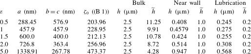
Simulation parameters for spheroidal particles with five different aspect ratios subject to three different confinements in a cylindrical tube with
 $D=5~\unicode[STIX]{x03BC}\text{m}$
and
 $L=40~\unicode[STIX]{x03BC}\text{m}$
. These parameters correspond to a particle orientation
 $\unicode[STIX]{x1D703}=90^{\circ }$
.

Appendix D. Mesh length on the particle used in the computation
The values of
 $l_{P}$
and
 $l_{W}$
(defined in figure 3) used in our calculations are given in table 4.
The mesh lengths on the particle and on the tubular wall,
 $l_{P}$
and
 $l_{W}$
, respectively, for five different aspect ratios and a confining wall with
 $D=5~\unicode[STIX]{x03BC}\text{m}$
and
 $L=40~\unicode[STIX]{x03BC}\text{m}$
.

Parameter values used in the calculation of drag and lift coefficients for comparison with that from Ouchene et al. (Reference Ouchene, Khalij, Taniere and Arcen2015).

Appendix E. Parameters used in the computation of drag and lift forces in the bulk
The target particle Reynolds number is computed as
 $Re_{p}(r)=|\boldsymbol{u}(r)|\,\text{d}_{eq}/\unicode[STIX]{x1D708}$
, where
 $d_{eq}$
is the equivalent sphere diameter and
 $\unicode[STIX]{x1D708}$
is the kinematic viscosity. We choose
 $\unicode[STIX]{x1D708}=10^{5}$
and particles with
 $a=5~\unicode[STIX]{x03BC}\text{m}$
and aspect ratios
 $\unicode[STIX]{x1D700}=5,2.5$
and
 $1.25$
. For each of the particles, we compute its equivalent sphere diameter as
 $d_{eq}=\sqrt[3]{abc}$
, see table 5 for details.