





1. Introduction
Porous media composed of a solid matrix with interconnected voids are ubiquitous in both natural environments and engineered systems (Bottaro Reference Bottaro2019). In geophysical settings such as granular beds and fractured formations, porous media govern groundwater migration (Goyal et al. Reference Goyal, Haritash and Singh2021) and control subsurface flow and transport in reservoirs (Guo et al. Reference Guo, Bandilla, Nordbotten, Celia, Keilegavlen and Doster2016). In engineering applications, porous structures formed by arrays of cylindrical elements arise in compact heat exchangers (Xie et al. Reference Xie, Zhao, Li and Wu2025a
), porous burners and combustion chambers (Wang et al. Reference Wang, Wang, Wang, Wang, Liu and Zhu2024), CO
 $_2$
geological storage (Huppert & Neufeld Reference Huppert and Neufeld2014) and thermal management devices (Zhao & Lu Reference Zhao and Lu2002), where pore-scale flow within the array directly controls pressure drop, heat and mass transfer, mixing and operational safety. Beyond these applications, porous media offer a canonical multiscale setting, in which the interplay of obstacle-induced shear and confinement governs the emergence of unsteadiness and the routes to transition.
Given the complex topology of porous media, numerical studies are essential for analysing flow instability and transitional phenomena. Numerical simulations of flow in porous media can be classified as either microscopic or macroscopic, depending on the time and length scales of the motions being resolved (Jin & Kuznetsov Reference Jin and Kuznetsov2024). Macroscopic simulations are performed by applying time and volume averaging to the microscopic governing equations (Wood et al. Reference Wood, He and Apte2020). In contrast, in microscopic simulations, flow phenomena at scales smaller than the representative elementary volume (REV) must be resolved (Jin et al. Reference Jin, Uth, Kuznetsov and Herwig2015), requiring explicit modelling of the detailed geometry of the porous elements. A commonly used approach is the generalised pore model, which consists of idealised solid obstacles such as cylinders, spheres or squares that approximate the local structure of the REV. Pore-scale-resolved simulations conducted on generalised pore model domains explicitly capture the pore-scale geometry and flow field, making this framework particularly suitable for investigating complex microscale phenomena in porous media, including the onset of flow instability and transition.
Compared with macroscopic studies, microscopic analyses have been relatively rare, primarily due to the greater geometrical complexity and higher computational cost. However, by capturing fine-scale flow structures, microscopic simulations can significantly enhance the understanding of flow behaviour in porous media. In particular, the global transition mechanism appears insensitive to specific microstructural configurations (Srikanth et al. Reference Srikanth, Huang, Su and Kuznetsov2021). To reduce computational cost, REV simulations are often performed in idealised periodic porous domains with periodic boundary conditions. For instance, Uth et al. (Reference Uth, Jin, Kuznetsov and Herwig2016) conducted direct numerical simulations (DNS) of isotropic porous media without volume-averaged assumptions, which fully resolve all flow scales. Chu et al. (Reference Chu, Weigand and Vaikuntanathan2018, Reference Chu, Yang, Pandey and Weigand2019) analysed turbulent kinetic energy transport and spectral features in square porous media with and without thermal convection. In addition, pore-resolved large-eddy simulations (Hutter et al. Reference Hutter, Zenklusen, Kuhn and Rudolf von Rohr2011; Shams et al. Reference Shams, Roelofs, Komen and Baglietto2014; Huang et al. Reference Huang, Srikanth and Kuznetsov2022) offer a good compromise between accuracy and efficiency, and the results generally agree with those of DNS (Chandesris et al. Reference Chandesris, D’Hueppe, Mathieu, Jamet and Goyeau2013; Rao & Jin Reference Rao and Jin2022). Notably, the macroscopic flow properties in REVs can also be inferred based on high-fidelity microscopic simulations (Wood et al. Reference Wood, He and Apte2020). For instance, Rao & Zhang (Reference Rao and Zhang2025) developed a coupled macroscopic model for forced thermal convection in periodic structures, with transport closures validated against pore-scale DNS. Very recently, the same authors further established unified scaling laws for vertical natural convection in porous media (Rao & Zhang Reference Rao and Zhang2026), enabling predictive macroscale modelling based on microscopic simulations.
Despite previous efforts, the complex interactions between fluid and solid phases make it challenging to clearly identify the various types of flow instabilities in porous media. Previous numerical and experimental studies have demonstrated that flow transition phenomena in porous structures can be highly complex (Koch & Hill Reference Koch and Hill2001). In a recent review, Wood et al. (Reference Wood, He and Apte2020) categorised the flow behaviour into four regimes as
 $\textit{Re}$
(the Reynolds number) increases:
 $(a)$
the Darcy regime,
 $(b)$
the inertial regime,
 $(c)$
the unsteady laminar (transitional) regime and
 $(d)$
the breakdown to turbulence. In particular, as the Reynolds number increases, a Hopf bifurcation may occur due to the oscillating wake behind the obstacles. From the perspective of hydrodynamic stability, the onset of the oscillatory instability is associated with a Hopf bifurcation, in which a steady fixed point loses stability as a complex-conjugate pair of eigenvalues of the linearised operator crosses the imaginary axis into the unstable half-plane (Schmid & Henningson Reference Schmid and Henningson2001; Frantz et al. Reference Frantz, Loiseau and Robinet2023). In the present study, this bifurcation corresponds to the onset of sustained unsteadiness from an initially steady pore-scale base flow and therefore defines the critical Reynolds number for the instability. Lahbabi & Chang (Reference Lahbabi and Chang1985) numerically investigated the transition in a cubic array of spheres and identified a Hopf bifurcation followed by period-doubling as the Reynolds number increased, before the flow eventually became chaotic. Similar phenomena have also been observed in the simulations of a spherical porous medium (Hill & Koch Reference Hill and Koch2002a
,
Reference Hill and Kochb
). Based on numerical and experimental studies, Mizushima & Akinaga (Reference Mizushima and Akinaga2003) demonstrated that the oscillatory flow induced by vortex shedding in a row of square bars originates from a Hopf bifurcation, offering physical insight into periodic instabilities in porous media structures. Sewatkar et al. (Reference Sewatkar, Sharma and Agrawal2009) showed that varying the gap ratio can induce transitions between synchronous and quasi-periodic flow regimes through secondary bifurcations. Bao et al. (Reference Bao, Wu and Zhou2012) studied flow past a six-cylinder inline array and found a sudden drop of the dominant frequency, indicating the onset of a Hopf bifurcation. Agnaou et al. (Reference Agnaou, Lasseux and Ahmadi2016) numerically investigated the first Hopf bifurcation for tandem or random placement of square and circular REVs, observing the transitional regime across a wide range of porosities. Very recently, for a set of tandem-arranged REV elements, Srikanth & Kuznetsov (Reference Srikanth and Kuznetsov2025a
,
Reference Srikanth and Kuznetsovb
) observed a Hopf bifurcation following symmetry breaking, with the resulting oscillatory behaviour interpreted as a secondary instability. Nevertheless, a theoretical explanation of the origin and underlying mechanisms of the phenomena is still lacking.
In addition to numerical and experimental investigations, stability and sensitivity analyses offer deeper theoretical insights into transition mechanisms such as symmetry breaking, vortex shedding and streak formation. As a general approach, global stability analysis is capable of capturing the full spatial complexity of flow instabilities and precisely identifying the critical transition parameters (Theofilis Reference Theofilis2011). Moreover, the receptivity of global modes to various modifications can be further quantified through adjoint-based sensitivity analysis (Sipp et al. Reference Sipp, Marquet, Meliga and Barbagallo2010). Common strategies, including structural sensitivity (i.e. the wavemaker) (Giannetti & Luchini Reference Giannetti and Luchini2007), sensitivity to base flow (Bottaro et al. Reference Bottaro, Corbett and Luchini2003) and sensitivity to forcing (Marquet et al. Reference Marquet, Sipp and Jacquin2008), provide direct guidance for flow control. For instance, Giannetti & Luchini (Reference Giannetti and Luchini2007) revealed that the most sensitive region in the wake of a single cylinder lies near the far downstream of the separation bubble. Pralits et al. (Reference Pralits, Brandt and Giannetti2010) extended this approach to a rotating cylinder and demonstrated suppression of vortex shedding using small control cylinders. In addition, Carini et al. (Reference Carini, Giannetti and Auteri2014) applied stability analysis to flows past side-by-side cylinders, a configuration analogous to wake interactions in REVs of cylinder arrays. Although global stability and sensitivity analyses have been extensively applied to canonical bluff-body flows (e.g. Williamson Reference Williamson1996; Barkley Reference Barkley2006; Yang et al. Reference Yang, Feng and Zhang2022; Nastro et al. Reference Nastro, Robinet, Loiseau, Passaggia and Mazellier2023; Frantz et al. Reference Frantz, Mimeau, Salihoglu, Loiseau and Robinet2025), their application to porous media remains limited, leaving an important gap in the understanding of flow transition in such systems.
Recently, Chu et al. (Reference Chu, Wu, Rist and Weigand2020) reported the first global stability analysis of transitional flows in elementary porous media. However, the study was restricted to staggered-arranged square cylinders with a fixed spacing and a few representative Reynolds numbers, leaving the transition pathways in elementary porous media not fully investigated. In particular, flow and heat transfer in porous media are commonly described in terms of porosity
 $\phi$
. Recent simulations suggest that macroscopic structures can survive within porous media only as
 $\phi$
approaches unity (Rao & Jin Reference Rao and Jin2022), which motivates us to investigate whether
 $\phi$
can be used to predict the onset threshold of unsteadiness based on microscopic simulations. Moreover, the role of REV geometry in the nature of instabilities has not been addressed. To develop a more complete picture of transition in porous media, the present study examines the global stability and bifurcation characteristics of tandem arrays of cylindrical obstacles over a range of porosities. Similar to the analysis of side-by-side cylinders in Carini et al. (Reference Carini, Giannetti and Auteri2014), we identify multiple eigenmode families with distinct spatial features, whose emergence is closely related to porosity. Notably, the critical Reynolds number for the Hopf bifurcation varies approximately linearly with
 $\phi$
at high and intermediate porosities, making it an effective diagnostic for predicting the instability onset. In addition, we explore adjoint-based sensitivity analysis and passive control, which highlights the regions where small base-flow modifications or localised forcing most effectively alter the stability characteristics.
The rest of the paper is organised as follows. Section 2 describes the flow configuration, governing equations, formulations of the stability and sensitivity analyses and numerical methods. Section 3 discusses the stability and bifurcation characteristics of the elementary porous media for different porosities. Section 4 presents a passive control strategy based on sensitivity analysis. Finally, discussions and conclusions are provided in § 5.
2. Problem formulation and numerical methods
2.1. Flow configuration
Schematic of the geometrical configuration and coordinate system. The region enclosed by the red dashed lines indicates the locally periodic computational domain used in the simulations, where periodic boundary conditions are imposed in all directions.

In the present study, a REV of a homogeneous porous medium composed of circular cylinders arranged in an inline configuration is simulated following Xie et al. (Reference Xie, Zhao, Ma, Li and Wu2025b
), as illustrated in figure 1. The computational domain consists of a doubly periodic array of circular cylinders with identical diameter
 $D$
, with adjacent cylinder surfaces separated by a gap
 $G$
in both the streamwise (
 $x$
) and transverse (
 $y$
) directions. Taking
 $D$
as the characteristic length scale gives
 $d=1$
, and the corresponding gap ratio is
 $g = G/D$
. The REV is defined as the central periodic unit cell of the array, corresponding to a computational domain of size
 $(3 +3g) \times (2 +2g)$
in the
 $x$
–
 $y$
plane, with periodic boundary conditions imposed in both directions. The enlarged computational domain enables the fundamental spatial period of the eigenmodes to be captured, thereby facilitating the identification of the leading stability characteristics. The flow is driven by imposing a mean pressure gradient in the streamwise (
 $x$
) direction to maintain a constant flow rate.
The governing equations of the flow are the incompressible, unsteady Navier–Stokes equations. In non-dimensional form:
 \begin{equation} \begin{cases} \partial _t\boldsymbol{U}+\boldsymbol{\nabla }\boldsymbol{U}\boldsymbol{\cdot }\boldsymbol{U}+\boldsymbol{\nabla }\!{P}-\textit{Re}^{-1}{\nabla} ^2\boldsymbol{U}= 0, \\[3pt] \boldsymbol{\nabla }\boldsymbol{\cdot }\boldsymbol{U} = 0, \end{cases} \end{equation}
where
 $\boldsymbol{U} = (U, V)$
represents the velocity,
 $P$
is the pressure and
 $\textit{Re}$
denotes the Reynolds number, which is defined based on
 \begin{equation} \textit{Re} = \frac {U_{\textit{int}} D}{\nu }. \end{equation}
where
 $\nu$
is the kinetic viscosity. Here
 $U_{\textit{int}}$
denotes the averaged interstitial velocity in the streamwise direction, given by
 \begin{equation} U_{\textit{int}} = \frac {\int _\varOmega U\, \mathrm{d}\varOmega }{\varOmega }, \end{equation}
in which
 $\varOmega = (3+3g)(2+2g) - 3\pi /2$
is the fluid area, where the second term accounts for the area occupied by the six circular cylinders within the REV.
To establish a connection between the pore-scale geometry and the macroscopic flow characteristics, the porosity
 $\phi$
is introduced as the fraction of void space (Anovitz & Cole Reference Anovitz and Cole2015). For the present two-dimensional configuration, the porosity is given by
 \begin{equation} \phi = 1 - \frac {\pi }{4(1+g)^2}. \end{equation}
It is also convenient to introduce the non-dimensional centre-to-centre spacing
 \begin{equation} \ell = 1+g, \end{equation}
so that (2.4) can be rewritten as
 \begin{equation} 1-\phi = \frac {\pi }{4\ell ^2}. \end{equation}
This relation provides a more direct geometric characterisation of the pore spacing, thereby facilitating a clearer interpretation of the transition threshold in the later discussion.
2.2. Linear stability analysis
We analyse the stability of the REV of the porous medium through global linear stability analysis, which evaluates the growth of infinitesimal perturbations to a base flow and determines the onset of instabilities and bifurcations. The steady base flow,
 $\boldsymbol{Q}_b = (\boldsymbol{U}_{\!b}, P_b)^T$
, is obtained as the steady-state solution of (2.1):
 \begin{equation} \begin{cases} \boldsymbol{\nabla }\boldsymbol{U}_{\!b}\boldsymbol{\cdot }\boldsymbol{U}_{\!b}+\boldsymbol{\nabla }\!{P}_b-\textit{Re}^{-1}{\nabla} ^2\boldsymbol{U}_{\!b}= 0,\\[3pt] \boldsymbol{\nabla }\boldsymbol{\cdot }\boldsymbol{U}_{\!b}=0. \end{cases} \end{equation}
An infinitesimal perturbation is then imposed on the base flow. Substituting the Reynolds decomposition
 $\boldsymbol{U} = \boldsymbol{U}_{\!b} + \boldsymbol{u}$
and
 $P = P_b + p$
into the governing equations (2.1) and neglecting high-order nonlinear terms, yields the linearised Navier–Stokes equations:
 \begin{equation} \begin{cases} \partial _t\boldsymbol{u}+\boldsymbol{\nabla }\boldsymbol{U}_{\!b} \boldsymbol{\cdot }\boldsymbol{u} + \boldsymbol{\nabla }\boldsymbol{u}\boldsymbol{\cdot }\boldsymbol{U}_{\!b} + \boldsymbol{\nabla }\!{p}-\textit{Re}^{-1}{\nabla} ^2\boldsymbol{u}=0,\\[3pt] \boldsymbol{\nabla }\boldsymbol{\cdot }\boldsymbol{u}=0, \end{cases} \end{equation}
where
 $\boldsymbol{u}$
and
 $p$
denote the velocity and pressure perturbations, respectively.
In linear modal stability analysis, the perturbation field is assumed to evolve exponentially in time:
 \begin{equation} \boldsymbol{q} = (\boldsymbol{u}, p)^T = \boldsymbol{\hat {q}}(x,y)e^{\lambda t} + \text{c.c.}, \end{equation}
where
 $\lambda$
denotes the complex temporal exponent and c.c. stands for the complex conjugate. Since the governing linearised problem has real coefficients, complex eigenvalues appear as conjugate pairs,
 $\sigma +{\rm i}\omega$
and
 $\sigma -{\rm i}\omega$
; the physical oscillation frequency is therefore given by
 $|\omega |/2\pi$
. Substituting the above normal-mode ansatz into the linearised Navier–Stokes equations (2.8) leads to a generalised eigenvalue problem:
 \begin{equation} \lambda \boldsymbol{M} \hat {\boldsymbol{q}} = \boldsymbol{A} \hat {\boldsymbol{q}}, \end{equation}
where
 $\boldsymbol{A}$
and
 $\boldsymbol{M}$
denote the Jacobian and the mass operators arising from the linearisation about the base state. The complex eigenvalue
 $\lambda = \sigma \pm {\rm i}\omega$
characterises the temporal evolution of the perturbation. The real part
 $\sigma$
denotes the growth rate, indicating whether perturbations intensify (
 $\sigma \gt 0$
) or decay (
 $\sigma \lt 0$
), whereas the absolute value of the imaginary part,
 $|\omega | = 2\pi f$
, represents the angular frequency associated with the oscillation frequency
 $f$
. Specifically, a flow is considered globally unstable if at least one growth rate becomes positive. In addition, the Strouhal number
 $\textit{St} = \textit{fd}/U_{\textit{int}}$
is introduced to characterise the frequency of vortex shedding. The corresponding eigenfunction
 $\hat {\boldsymbol{q}}$
, referred to as the eigenmode, represents the spatial structure of the instability.
2.3. Adjoint-based sensitivity analysis and flow control
The introduction of adjoint equations for sensitivity analysis allows a detailed identification of the regions governing the onset and evolution of flow instability mechanisms. The adjoint problem can be obtained through the generalised Lagrange identity, which defines the dual of the linearised Navier–Stokes operator,
 $\mathcal{L}^+$
, such that
 \begin{equation} \left \langle \boldsymbol{q}^+, \mathcal{L} \boldsymbol{q} \right \rangle = \left \langle \mathcal{L}^+ \boldsymbol{q}^+, \boldsymbol{q} \right \rangle \!, \end{equation}
for any admissible perturbation state
 $\boldsymbol{q}^+$
. The adjoint mode can be obtained by solving the eigenvalue problem for the adjoint operator, analogous to the direct problem (2.10). The adjoint eigenproblem is defined with respect to the
 $L^2$
inner product
 \begin{equation} \langle \boldsymbol{q}^+, \boldsymbol{q} \rangle = \int _{\varOmega } \boldsymbol{q}^{+*}\boldsymbol{\cdot }\boldsymbol{q}\,\mathrm{d}\varOmega , \end{equation}
where the asterisk denotes the complex conjugate. The direct and adjoint modes are normalised using the corresponding bi-orthogonality condition
 \begin{equation} \langle \boldsymbol{q}^+, \boldsymbol{q} \rangle = 1. \end{equation}
In addition, the structural sensitivity, referred to as the wavemaker (Giannetti & Luchini Reference Giannetti and Luchini2007), is given by
 \begin{equation} S = |\boldsymbol{q}|\,|\boldsymbol{q}^+|, \end{equation}
which identifies the core region of the instability and is of particular interest in the development of flow-control strategies. Under the present bi-orthogonal normalisation, the wavemaker field is evaluated as the pointwise product of the local amplitudes of the direct and adjoint modes.
Furthermore, effective passive control strategies can be designed based on the sensitivities to base-flow modifications or external forcing. By constructing a Lagrangian functional based on the direct and adjoint eigenvalue problems, the sensitivity of the eigenvalue
 $\lambda$
to the base flow
 $\boldsymbol{U}_{\!b}$
is obtained by taking variations of the functional with respect to
 $\boldsymbol{U}_{\!b}$
:
 \begin{equation} \boldsymbol{\nabla} _{\!\boldsymbol{U}_{\!b}} \lambda = \underbrace {-(\boldsymbol{\nabla }\boldsymbol{\hat {u}})^H \boldsymbol{\cdot }\boldsymbol{\hat {u}}^+}_{\boldsymbol{\nabla} _{\boldsymbol{U}_{\!b},T}\lambda } + \underbrace {\boldsymbol{\nabla }\boldsymbol{\hat {u}}^+ \boldsymbol{\cdot }\boldsymbol{\hat {u}}^*}_{\boldsymbol{\nabla} _{\boldsymbol{U}_{\!b},P}\lambda }, \end{equation}
in which the superscript
 ${}^{H}$
denotes the Hermitian transpose. As discussed in Marquet et al. (Reference Marquet, Sipp and Jacquin2008), the two contributions
 $\boldsymbol{\nabla} _{\boldsymbol{U}_{\!b},T}\lambda$
and
 $\boldsymbol{\nabla} _{\boldsymbol{U}_{\!b},P}\lambda$
can be interpreted as the sensitivity to modifications of perturbation transport, and of perturbation production, by the base flow.
Similarly, the sensitivity to steady forcing can be derived by taking variations of the Lagrangian functional with respect to an external forcing
 $\boldsymbol{F}$
, leading to the equations for adjoint base flow
 \begin{equation} -\boldsymbol{\nabla }\boldsymbol{U}_{\!b}^+ \boldsymbol{\cdot }\boldsymbol{U}_{\!b} + (\boldsymbol{\nabla }\boldsymbol{U}_{\!b})^T \boldsymbol{\cdot }\boldsymbol{U}_{\!b}^+ -\boldsymbol{\nabla }\!P_b^+ -\textit{Re}^{-1}{\nabla} ^2\boldsymbol{U}_{\!b}^+ = \boldsymbol{\nabla} _{\!\boldsymbol{U}_{\!b}}\lambda , \qquad \boldsymbol{\nabla }\boldsymbol{\cdot }\boldsymbol{U}_{\!b}^+=0 . \end{equation}
Then the sensitivity to steady forcing is directly given by the adjoint base flow
 $\boldsymbol{\nabla} _{\!\boldsymbol{F}} \lambda =\boldsymbol{U}_{\!b}^+$
. Detailed derivations of the sensitivity equations can be found in Marquet et al. (Reference Marquet, Sipp and Jacquin2008).
From the perspective of flow control, the eigenvalue drift induced by adding a small forcing perturbation
 $\delta \boldsymbol{F}$
to the governing equations can be computed as
 $\delta \lambda _{\textit{stability}} = \lambda _{\delta \boldsymbol{F}\neq 0} - \lambda _{\delta \boldsymbol{F}=0}$
, or evaluated directly from
 \begin{equation} \delta \lambda _F = \left \langle \boldsymbol{\nabla} _{\!\boldsymbol{F}} \lambda \,\middle |\, \delta \boldsymbol{F} \right \rangle \!. \end{equation}
Accordingly, the sensitivity gradient provides an effective means of assessing the impact of flow control without the need to perform the stability analysis again.
Moreover, note that since evaluating the sensitivity to a steady force requires
 $\boldsymbol{\nabla} _{\!\boldsymbol{U}_{\!b}}\lambda$
,
 $\delta \boldsymbol{F}$
may equivalently be interpreted in terms of the associated base-flow modification
 $\delta \boldsymbol{U}_{\!\boldsymbol{F}} = \boldsymbol{\nabla} _{\!\boldsymbol{F}} \boldsymbol{U}_{\!b} \boldsymbol{\cdot }\delta \boldsymbol{F}$
. In analogy with (2.17), the corresponding eigenvalue variation is given by
 \begin{equation} \delta \lambda _{U_b} = \big \langle \boldsymbol{\nabla} _{\!\boldsymbol{U}_{\!b}} \lambda \,\big |\, \delta \boldsymbol{U}_{\!\boldsymbol{F}} \big \rangle . \end{equation}
Therefore, the variation
 $\delta \lambda$
induced by external forcing can be determined either by repeating the stability analysis after introducing
 $\delta \boldsymbol{F}$
, or, equivalently but more efficiently, from the sensitivity functions
 $\boldsymbol{\nabla} _{\!\boldsymbol{F}} \lambda$
or
 $\boldsymbol{\nabla} _{\!\boldsymbol{U}_{\!b}}\lambda$
.
2.4. Perturbation kinetic energy analysis
The instability mechanisms can also be examined from an energy transfer perspective by identifying the sources of perturbation amplification using the perturbation kinetic energy (PKE) budget derived from the Reynolds–Orr equation:
 \begin{equation} \frac {\mathrm{d}\textit{E}}{\mathrm{d}\textit{t}} = \int _{\varOmega } I_i \, \mathrm{d}\varOmega - \int _{\varOmega } \textit{D} \, \mathrm{d}\varOmega , \end{equation}
where
 $E = ({1}/{2})\int _{\varOmega } u_i^2 \, \mathrm{d}\varOmega$
denotes the PKE. Specifically, the production term
 \begin{equation} I_i = -\,u_i u_j \frac {\partial U_{b,i}}{\partial x_j} \end{equation}
quantifies the rate of energy transfer from the mean flow to the disturbances, while the dissipation term is
 \begin{equation} D = \frac {1}{\textit{Re}}\,\frac {\partial u_i}{\partial x_k}\frac {\partial u_i}{\partial x_k}, \end{equation}
which represents the viscous removal of perturbation energy. The formulation quantifies perturbation energy production and dissipation, identifying where and how a mode extracts energy from the base flow and drives instability. Accordingly, PKE analysis complements linear stability and sensitivity analyses by revealing the energy pathways responsible for disturbance amplification.
Specifically,
 $I_i$
can be further decomposed into four components:
 \begin{equation} I_1=-u^2 \frac {\partial U_b}{\partial x},\qquad I_2=-u v \frac {\partial U_b}{\partial y},\qquad I_3=-v u \frac {\partial V_b}{\partial x},\qquad I_4=-v^2 \frac {\partial V_b}{\partial y}. \end{equation}
Each term corresponds to a distinct physical mechanism associated with the in-plane velocity gradients of the base flow, thereby helping to elucidate the origin of the observed instabilities. Specifically,
 $I_1$
represents the contribution due to streamwise acceleration and deceleration of the base flow within the porous medium. The term
 $I_2$
reflects the lift-up mechanism, where wall-normal perturbations interact with the base-flow shear to induce amplification of streamwise streaks. The contribution
 $I_3$
quantifies energy transfer associated with streamwise variations of the lateral component of the base flow. Finally,
 $I_4$
corresponds to the converging–diverging mechanism in the lateral direction.
2.5. Numerical methods
In order to perform high-fidelity numerical simulations and stability analyses of the porous medium composed of circular cylinders, high-order spectral element codes Nek5000 (Fischer et al. Reference Fischer, Kerkemeier and Peplinski2020) are used. The time step
 $\Delta t$
is selected to satisfy the Courant–Friedrichs–Lewy condition, with the Courant number maintained between 0.5 and 1.0. A polynomial order
 $N=7$
is adopted to balance accuracy and computational cost, following the recommendations of Fischer et al. (Reference Fischer, Kerkemeier and Peplinski2020). Grid refinement is applied near boundary layers, in which the elements have been refined by the O-type mesh (see figure 1). The combination of mesh flexibility and spectral accuracy makes the current computational approach well suited for handling complex geometries. The unit cell is subject to periodic boundary conditions on opposite faces, with the velocity and the periodic component of pressure taken to be periodic. The flow rate is fixed by prescribing the non-dimensional mean streamwise velocity
 $U_{\textit{int}} = 1$
for all geometrical configurations, while the mean pressure gradient is adjusted during the computation to maintain the prescribed bulk flow.
The base flows for stability analysis are computed using a fully converged Newton–Krylov method. The linear systems are solved based on a generalised minimal residual (GMRES) algorithm, and Newton iterations are advanced until the absolute residual falls below
 $10^{-11}$
, ensuring accuracy and robustness in subsequent stability analysis. The global stability and sensitivity analyses are performed through matrix-free eigenvalue computations in Krylov subspace. A residual tolerance of
 $10^{-7}$
is imposed as the stopping criterion in the Arnoldi iteration for the generalised eigenvalue problem. For the linearised problem, the perturbation fields are subject to the same periodic boundary conditions on the paired boundaries of the REV, while homogeneous no-slip conditions are imposed on the cylinder surfaces. The bulk-flow constraint used to obtain the base state is not applied separately in the perturbation eigenvalue problem. For each case, we compute the eight leading eigenmodes and rank them by growth rate to identify the dominant instability. The relevant physical branches are then tracked across the parameter space based on the continuity of eigenvalue evolution, oscillation frequency and eigenmode structure. For the detailed numerical implementations, the reader is referred to Yang et al. ( Reference Yang, Feng and Zhang2022, Reference Yang, Wang, Guo and Zhang2023). Additional validations of the numerical methods and grid sensitivity analyses for DNS and eigenvalue computations are provided in Appendix A. Moreover, a justification for restricting the stability analysis to two dimensions is given in Appendix B.
3. Stability and bifurcation analysis
In this section, we examine the global stability and bifurcation behaviour of the present tandem-cylinder REV over a wide range of porosities. We first determine the threshold trends and the dominant eigenmodes of the leading Hopf bifurcation, and then analyse the instability core and its sustaining mechanism via structural sensitivity and perturbation energy analysis.
3.1. Base flow
The converged base flows at the critical Reynolds number for several representative spacings
 $g$
are shown in figure 2. In all cases, the maximum streamwise velocity occurs in the throat between the two cylinders, where the tandem arrangement induces minimal velocity loss and yields flow characteristics analogous to those of a channel flow. For low-
 $g$
cases, wake development is strongly suppressed due to the geometric confinement of the neighbouring obstacles. As the gap increases, the streamwise velocity decreases both in the throat and in the recirculation region. The base flow provides the basis for the stability analysis in the following sections.
3.2. Global modes and bifurcations
Streamwise velocity field of the base flow at the critical Reynolds number for different gap spacings:
 $(a)$
 $g = 0.2$
at
 $\textit{Re} = 303.4$
,
 $(b)$
 $g = 0.4$
at
 $\textit{Re} = 219.1$
,
 $(c)$
 $g = 0.6$
at
 $\textit{Re} = 142.6$
,
 $(d)$
 $g = 0.8$
at
 $\textit{Re} = 90.7$
,
 $(e)$
 $g = 1.2$
at
 $\textit{Re} = 38.8$
,
 $(f)$
 $g = 1.4$
at
 $\textit{Re} = 31$
,
 $(g)$
 $g = 1.6$
at
 $\textit{Re} = 26.2$
,
 $(h)$
 $g = 1.8$
at
 $\textit{Re} = 22.8$
.

Variations of the critical Reynolds number
 ${\textit{Re}}_c$
and the linear stability analysis eigenfrequency
 $\omega /2\pi$
as functions of
 $(a)$
the gap ratio
 $g$
and
 $(b)$
the porosity
 $\phi$
.

Streamwise spatial distribution of the direct modes of the leading eigenvalue at the critical Reynolds number
 ${\textit{Re}}_c$
for different gap spacings:
 $(a)$
 $g = 0.2$
at
 $\textit{Re} = 303.4$
(APS mode),
 $(b)$
 $g = 0.3$
at
 $\textit{Re} = 255.9$
(APL mode),
 $(c)$
 $g = 0.4$
at
 $\textit{Re} = 219.1$
(IPS mode),
 $(d)$
 $g = 0.6$
at
 $\textit{Re} = 142.6$
(IPM mode),
 $(e)$
 $g = 1.0$
at
 $\textit{Re} = 55.1$
(IPL mode),
 $(f)$
 $g = 1.6$
at
 $\textit{Re} = 26.2$
(IPL mode).

To identify the transition threshold of the present elementary porous-medium configuration, figure 3 summarises the critical Reynolds number
 ${\textit{Re}}_c$
and the corresponding frequency over the range of porosities considered. As in the wake of a single circular cylinder (Williamson Reference Williamson1996), the primary instability of the present REV is dominated by two-dimensional modes, as verified in Appendix A. In all cases, the leading eigenmodes have non-zero frequency, indicating a Hopf bifurcation. Following Kang (Reference Kang2003) for side-by-side cylinders, the dominant instability may be classified as an in-phase (IP) or an anti-phase (AP) synchronised mode according to its symmetry. In addition, the frequencies within each colour-coded region in figure 3 show only small variations. The corresponding spatial periods are integer multiples of the minimal periodic unit (see figure 4), and the oscillation frequency differs markedly between different branches. Accordingly, the IP modes are further subdivided into IPL, IPM and IPS, corresponding to long-, intermediate- and short-period structures, respectively. The AP modes are likewise classified into APL and APS. Specifically, the unstable modes in figures 4
 $(a)$
and 4
 $(b)$
differ from those in the remaining panels and exhibit a symmetry about the horizontal axis. By contrast, the other modes show nearly identical structures in the upper and lower channels, indicative of IP synchronised vortex shedding (Carini et al. Reference Carini, Giannetti and Auteri2014). Apparently, the AP modes can be attributed to strong mutual interference and phase coupling between the separated shear layers. When the gap is sufficiently narrow, the shear layers interact strongly across the throat, enabling efficient exchange of vorticity and pressure perturbations and promoting AP synchronisation between the upper and lower channels at a dominant frequency. As the gap increases, the cross-gap coupling is progressively reduced, so that the upper and lower channels become increasingly decoupled and behave more like two separate wakes. Consequently, the global mode becomes closer to that of a confined channel flow (Schmid & Henningson Reference Schmid and Henningson2001). The leading response shifts towards an IP organisation, indicating that the spacing ratio and the associated porosity are key parameters controlling the instability.
Neutral stability curves in the
 $\phi$
–
 $\textit{Re}$
plane. The grey region denotes the stable regime. The colours of the neutral curves indicate different dominant unstable modes: APS (purple,
 $\phi \lt 0.5069$
), APL (blue,
 $0.5069 \leqslant \phi \lt 0.5840$
), IPS (green,
 $0.5840 \leqslant \phi \lt 0.6605$
), IPM (orange,
 $0.6605 \leqslant \phi \lt 0.7725$
) and IPL (red,
 $\phi \geqslant 0.7725$
). The
 ${\textit{Re}}_c$
values obtained from two-dimensional (2-D) DNS and tri-global stability analysis are denoted by open square and cross symbols, respectively. The remaining data points are obtained from bi-global stability analysis with spanwise wavenumber
 $k_z=0$
.

Neutral stability curves in the
 $g$
–
 $\textit{Re}$
plane. The grey region denotes the stable regime. The colours of the neutral curves indicate different dominant unstable modes: APS (purple,
 $g \lt 0.262$
), APL (blue,
 $0.262 \leqslant g \lt 0.347$
), IPS (green,
 $0.347 \leqslant g \lt 0.521$
), IPM (orange,
 $0.521 \leqslant g \lt 0.858$
) and IPL (red,
 $g \geqslant 0.858$
). The
 ${\textit{Re}}_c$
values obtained from two-dimensional (2-D) DNS and tri-global stability analysis are denoted by open square and cross symbols, respectively. The remaining data points are obtained from bi-global stability analysis with spanwise wavenumber
 $k_z=0$
.

Note that the critical Reynolds numbers
 ${\textit{Re}}_c$
associated with the AP mode are significantly higher than those at larger spacings. Over the porosity range considered in the present work,
 ${\textit{Re}}_c$
decreases monotonically with increasing gap ratio, reflecting progressively weaker shear-layer confinement and therefore an earlier onset of the primary instability. A simple scaling argument for
 ${\textit{Re}}_c$
can be formulated in terms of competing advective and viscous time scales. Near onset, the growth rate
 $\sigma$
quantifies the temporal growth of the instability and is therefore taken to scale with the inverse advective time,
 $\sigma \sim U_{\textit{int}}/D$
. Additionally, based on the non-dimensional centre-to-centre spacing
 $\ell$
defined in (2.5), a natural estimate for the pore length scale is
 $L\sim \ell D$
. Viscous effects then enter through momentum diffusion across a pore, giving a damping rate
 $\sigma _\nu \sim \nu /L^2\sim \nu /(\ell ^2D^2)$
. Balancing the two effects at criticality gives
 \begin{equation} \frac {U_{\textit{int}}}{D}\sim C\,\frac {\nu }{\ell ^2D^2}, \end{equation}
where
 $C=O(1)$
depends on the detailed modal structure and feedback mechanism. Rearranging yields
 \begin{equation} {\textit{Re}}_c = \frac {U_{\textit{int}}D}{\nu }\sim \frac {C}{\ell ^2}. \end{equation}
Then based on (2.6),
 \begin{equation} {\textit{Re}}_c\sim A(1-\phi )=A-A\phi , \end{equation}
suggesting a linear dependence of the transition threshold on porosity. The trend is indeed apparent in figures 5 and 6. The threshold of the Hopf bifurcation varies in a piecewise-linear manner with the porosity
 $\phi$
. A linear fit yields
 \begin{equation} {\textit{Re}}_c(\phi )= \begin{cases} -733.2\phi + 649.6, \quad \text{ for } \quad 0.45 \lt \phi \lesssim 0.8,\\[3pt] -205.8\phi + 208.7, \quad \text{ for } \quad 0.85 \lesssim \phi \lt {0.95}, \end{cases} \end{equation}
with a coefficient of determination
 $R^2$
exceeding
 $0.99$
in both cases. The breakpoint selection was assessed using the refined dataset in the transition region. The endpoints of the two fitting branches were varied point by point from the minimum- and maximum-porosity sides, and a linear regression was performed for each candidate endpoint. Since several nearby endpoints for the low-porosity branch gave almost unchanged values of
 $R^2$
, we selected the integer-spacing case
 $g=1$
, corresponding to
 $\phi =0.804$
, as the endpoint because of its clearer geometric interpretation. For the high-porosity branch, the starting point was selected using the same
 $R^2$
criterion, giving the case
 $g=1.3$
, corresponding to
 $\phi =0.851$
. This procedure suggests that the breakpoint represents a narrow transition region rather than a mathematically sharp value. The fitted results are also consistent with the trends shown in figure 6, which reflect the corresponding inverse-square dependence on spacing. The linear stability analysis yields a transition threshold that is consistent with the DNS-based estimate, with details of the estimation procedure given in Appendix C (see also Yang et al. Reference Yang, Wang, Guo and Zhang2023). Additional tri-global stability calculations show that the critical conditions are consistent with those obtained from the bi-global analysis, indicating that the instability onset is dominated by the two-dimensional mode in the present parameter range. The detailed validation procedure is reported in Appendix B. The Landau coefficient obtained from the weakly nonlinear analysis further indicates that the bifurcation is supercritical across the considered parameter range. Together, these findings show that the present global stability analysis accurately captures the instability onset and that porosity can be regarded as a key indicator of transition.
The PKE production terms
 $\int _\varOmega I_i \,\mathrm{d} \varOmega$
for different gap values
 $g$
, in which
 $I_{\textit{sum}} = \sum _{n=1}^4 I_n$
.

The change in scaling across porosity regimes can be attributed to a shift in the dominant length scale and coupling mechanism inside the REV. Recent pore-resolved simulations indicate that the internal flow remains dominated by pore-scale motions, as macroscale vortical structures collapse rapidly upon entering the porous media (Courter et al. Reference Courter, Srikanth, Kemayo and Kuznetsov2026). At lower porosities, the pore geometry thus plays a primary role in determining the flow structure and the transition behaviour. Accordingly, the present results show an approximately linear variation of the Hopf threshold with
 $\phi$
over
 $0.45 \lesssim \phi \lesssim 0.8$
. In addition, a second, shorter linear segment is also observed at higher porosities (
 $\phi \gtrsim 0.85$
), albeit with a different slope. At high porosity, wake interference is reduced and the variation of
 ${\textit{Re}}_c$
with
 $\phi$
becomes weaker as the flow moves towards the isolated-cylinder limit, at which one would recover the classical onset of vortex shedding for an isolated cylinder,
 ${\textit{Re}}_c \approx 47$
(Barkley Reference Barkley2006). Nevertheless, even at the highest porosity considered here (
 $\phi =0.95$
), the primary threshold remains substantially smaller (
 ${\textit{Re}}_c=13.2$
). The phenomenon indicates that the REV does not simply approach the unbounded single-cylinder limit, since residual confinement and periodic interactions can still provide an efficient global feedback that precipitates an earlier onset of Hopf bifurcation. The intermediate interval
 $0.8 \lesssim \phi \lesssim 0.85$
can therefore be considered as a buffer regime, in which the instability reorganises from a strongly coupled, throat-controlled dynamics towards a more wake-dominated behaviour. The resulting competition between coupling mechanisms naturally produces a gradual change in slope between the two approximately linear branches.
3.3. Perturbation energy analysis and wavemaker
The PKE distributions
 $I_{\textit{sum}} = \sum _{n=1}^4 I_n$
of the leading direct mode at
 $(a)$
 $g = 0.2$
,
 ${\textit{Re}}_c = 303.4$
,
 $(b)$
 $g = 0.3$
,
 ${\textit{Re}}_c = 255.9$
,
 $(c)$
 $g = 0.4$
,
 ${\textit{Re}}_c = 219.1$
,
 $(d)$
 $g = 0.6$
,
 ${\textit{Re}}_c = 142.6$
,
 $(e)$
 $g = 1.0$
,
 ${\textit{Re}}_c = 55.1$
and
 $(f)$
 $g = 1.6$
,
 ${\textit{Re}}_c = 26.2$
.

The wavemaker of the leading eigenmode at
 $(a)$
 $g = 0.2$
,
 ${\textit{Re}}_c = 303.4$
,
 $(b)$
 $g = 0.3$
,
 ${\textit{Re}}_c = 255.9$
,
 $(c)$
 $g = 0.4$
,
 ${\textit{Re}}_c = 219.1$
,
 $(d)$
 $g = 0.6$
,
 ${\textit{Re}}_c = 142.6$
,
 $(e)$
 $g = 1.0$
,
 ${\textit{Re}}_c = 55.1$
and
 $(f)$
 $g = 1.6$
,
 ${\textit{Re}}_c = 26.2$
.

Figure 9. Long description
Panel A: A heat map showing flow instability patterns around circular objects. The horizontal axis ranges from -1.8 to 1.8, and the vertical axis ranges from -1.2 to 1.2. The color scale ranges from -2.50 to 2.50. Panel B: A heat map showing flow instability patterns around circular objects. The horizontal axis ranges from -1.95 to 1.95, and the vertical axis ranges from -1.30 to 1.30. The color scale ranges from -2.00 to 2.00. Panel C: A heat map showing flow instability patterns around circular objects. The horizontal axis ranges from -2.1 to 2.1, and the vertical axis ranges from -1.4 to 1.4. The color scale ranges from -1.00 to 1.00. Panel D: A heat map showing flow instability patterns around circular objects. The horizontal axis ranges from -2.4 to 2.4, and the vertical axis ranges from -1.6 to 1.6. The color scale ranges from -0.80 to 0.80. Panel E: A heat map showing flow instability patterns around circular objects. The horizontal axis ranges from -3.0 to 3.0, and the vertical axis ranges from -2.0 to 2.0. The color scale ranges from -0.60 to 0.60. Panel F: A heat map showing flow instability patterns around circular objects. The horizontal axis ranges from -3.9 to 3.9, and the vertical axis ranges from -2.6 to 2.6. The color scale ranges from -0.40 to 0.40.
The instability mechanism is further elucidated by examining the PKE budget evaluated for the dominant global eigenmode. As summarised in figure 7, the production is dominated by the lift-up contribution
 $I_2$
. As
 $g$
increases, the amplitude of
 $I_2$
decreases but remains dominant over other terms. By comparison,
 $I_1$
,
 $I_3$
and
 $I_4$
are small in the integrated balance, indicating that these terms primarily redistribute perturbation energy locally rather than contributing to the net production. As outlined in § 2.4, the production is separated into contributions associated with the streamwise and cross-stream gradients of the base flow. The instability is therefore mainly shear-driven, with lift-up mechanism converting cross-stream motion into amplified streamwise streaks (Brandt Reference Brandt2014). A similar predominance of the lift-up mechanism in the production budget has also been reported in related geometries (Lashgari et al. Reference Lashgari, Tammisola, Citro, Juniper and Brandt2014; Chu et al. Reference Chu, Wu, Rist and Weigand2020).
In addition, the spatial distribution of the total PKE production is compared across different gaps in figure 8. Specifically, for relatively small gap
 $g=0.2$
, positive production peaks upstream of the channel and extends into the downstream region of the upstream cylinder, whereas negative
 $I_{\textit{sum}}$
remains confined near the cylinder walls and is largely balanced by the other contributions. Overall, the positive contribution of
 $I_{\textit{sum}}$
clearly outweighs its negative counterpart, indicating that the corresponding lift-up mechanism plays a dominant role in promoting the flow instability.
To further identify the core of the global instability, we perform structural sensitivity analysis based on the overlap of the normalised direct and adjoint modes (Giannetti & Luchini Reference Giannetti and Luchini2007), as depicted in figure 9. The wavemaker highlights where the local feedback sustaining the global mode is strongest. For all cases, the sensitivity concentrates in two symmetric bands along the passage between the tandem cylinders and extends into the near wake. These regions closely coincide with the maxima of the total production
 $I_{\textit{sum}}$
in figure 8, linking the energetic diagnosis to the sensitivity-based identification of the instability core.
As the gap
 $g$
(and hence the porosity
 $\phi$
) increases, the regions of significant PKE production and wavemaker intensity broaden as geometric confinement relaxes. Over the entire range considered, the net energy production remains dominated by the lift-up mechanism, whose positive regions broaden laterally and penetrate further into the recirculation zones, whereas the region with vanishing production along the channel centre also widens. The wavemaker exhibits a similar evolution. As the porosity increases, the high-sensitivity bands along the main passage widen and extend further into the near wake, while their peak intensity decreases. This indicates that the dominant unsteadiness becomes less responsive to localised perturbations, despite the preferred locations remaining tied to the shear amplification region. At the largest gap (see figure 9
 $f$
), the wavemaker becomes more spatially uniform, with sensitivity distributed over a larger fraction of the domain. Overall, the wavemaker distribution remains closely aligned with the regions of strongest PKE production, motivating the subsequent design of control strategies.
4. Flow control
In addition to global stability analysis, we further implement the adjoint-based framework outlined in § 2.3 to control the onset of instability. We show that the sensitivity-based estimates are capable of capturing both the growth rate and frequency shifts obtained from global stability analysis for the present REV of porous media, providing practical guidance for control design.
Streamwise spatial distributions of the growth rate sensitivity of the leading eigenvalue to base-flow modifications at the critical Reynolds number
 ${\textit{Re}}_c$
, for different gap ratios
 $g$
:
 $(a)$
 $g=0.2$
,
 $(b)$
 $g=0.3$
,
 $(c)$
 $g=0.4$
,
 $(d)$
 $g=0.6$
,
 $(e)$
 $g=1.0$
,
 $(f)$
 $g=1.6$
.

4.1. Sensitivity to base-flow modifications
We first examine the sensitivity of the leading global mode to perturbations of the base flow. The corresponding sensitivities of the growth rate
 $\sigma$
and frequency
 $\omega$
are reported in figures 10 and 11, respectively. Similar to the changes observed in the leading eigenmodes, the sensitivity gradient varies markedly with
 $g$
. For relatively low porosities,
 $\boldsymbol{\nabla} _{\!\boldsymbol{U}_{\!b}}\sigma$
is positive along the centreline of the channels and near the cylinder edges, implying that an increase of base-flow velocity in the core and near-wall regions promotes instability. Conversely, negative sensitivity appears between these zones, motivating a careful choice of control targets. As the gap opens, the positive sensitivity in the passage core decreases, consistent with the reduced influence of wall effects, whereas the positive region near the cylinders prior to separation persists and expands. In the meantime, negative sensitivity occupies an increasing fraction of the wake, suggesting that the instability mechanism gradually reorganises from a confinement-induced mode towards a more canonical cylinder wake character.
The frequency sensitivity
 $\boldsymbol{\nabla} _{\!\boldsymbol{U}_{\!b}}\omega$
in figure 11 follows the same overall trend with porosity, although the specific sensitive regions differ. In particular, negative contributions to
 $\omega$
are more tightly localised to the throat between the cylinders. At larger
 $g$
, a second confined negative patch appears immediately behind each cylinder, whereas most of the wake exhibits positive sensitivity, indicating that locally increasing the mean flow over much of the wake tends to raise the frequency, which again highlights the importance of control placement.
Streamwise spatial distributions of the frequency sensitivity of the leading eigenvalue to base-flow modifications at the critical Reynolds number
 ${\textit{Re}}_c$
, for different gap ratios
 $g$
:
 $(a)$
 $g=0.2$
,
 $(b)$
 $g=0.3$
,
 $(c)$
 $g=0.4$
,
 $(d)$
 $g=0.6$
,
 $(e)$
 $g=1.0$
,
 $(f)$
 $g=1.6$
.

Figure 11. Long description
Panel A: A heat map shows the streamwise spatial distribution of frequency sensitivity for a gap ratio of 0.2. The x-axis ranges from -1.8 to 1.8, and the y-axis ranges from -1.2 to 1.2. The color scale ranges from -40.0 to 40.0. Panel B: A heat map shows the streamwise spatial distribution of frequency sensitivity for a gap ratio of 0.4. The x-axis ranges from -1.95 to 1.95, and the y-axis ranges from -1.3 to 1.3. The color scale ranges from -20.0 to 20.0. Panel C: A heat map shows the streamwise spatial distribution of frequency sensitivity for a gap ratio of 0.6. The x-axis ranges from -2.1 to 2.1, and the y-axis ranges from -1.4 to 1.4. The color scale ranges from -10.0 to 10.0. Panel D: A heat map shows the streamwise spatial distribution of frequency sensitivity for a gap ratio of 0.8. The x-axis ranges from -2.4 to 2.4, and the y-axis ranges from -1.6 to 1.6. The color scale ranges from -10.0 to 10.0. Panel E: A heat map shows the streamwise spatial distribution of frequency sensitivity for a gap ratio of 1.0. The x-axis ranges from -3.0 to 3.0, and the y-axis ranges from -2.0 to 2.0. The color scale ranges from -2.0 to 2.0. Panel F: A heat map shows the streamwise spatial distribution of frequency sensitivity for a gap ratio of 1.2. The x-axis ranges from -3.9 to 3.9, and the y-axis ranges from -2.6 to 2.6. The color scale ranges from -0.50 to 0.50.
4.2. Sensitivity to a steady force
Streamwise spatial distributions of the growth rate sensitivity of the leading eigenvalue to a steady force at the critical Reynolds number
 ${\textit{Re}}_c$
, for different gap ratios
 $g$
:
 $(a)$
 $g=0.2$
,
 $(b)$
 $g=0.3$
,
 $(c)$
 $g=0.4$
,
 $(d)$
 $g=0.6$
,
 $(e)$
 $g=1.0$
,
 $(f)$
 $g=1.6$
.

Streamwise spatial distributions of the frequency sensitivity of the leading eigenvalue to a steady force at the critical Reynolds number
 ${\textit{Re}}_c$
, for different gap ratios
 $g$
:
 $(a)$
 $g=0.2$
,
 $(b)$
 $g=0.3$
,
 $(c)$
 $g=0.4$
,
 $(d)$
 $g=0.6$
,
 $(e)$
 $g=1.0$
,
 $(f)$
 $g=1.6$
.

Figure 13. Long description
Panel A: A heat map showing streamwise spatial distributions of the frequency sensitivity of the leading eigenvalue to a steady force at the critical Reynolds number for a gap ratio of 0.2. The x-axis ranges from -1.8 to 1.8, and the y-axis ranges from -1.2 to 1.2. The color scale ranges from -5.00 to 5.00. Panel B: A heat map showing streamwise spatial distributions of the frequency sensitivity of the leading eigenvalue to a steady force at the critical Reynolds number for a gap ratio of 0.3. The x-axis ranges from -1.95 to 1.95, and the y-axis ranges from -1.30 to 1.30. The color scale ranges from -5.00 to 5.00. Panel C: A heat map showing streamwise spatial distributions of the frequency sensitivity of the leading eigenvalue to a steady force at the critical Reynolds number for a gap ratio of 0.4. The x-axis ranges from -2.1 to 2.1, and the y-axis ranges from -1.4 to 1.4. The color scale ranges from -5.00 to 5.00. Panel D: A heat map showing streamwise spatial distributions of the frequency sensitivity of the leading eigenvalue to a steady force at the critical Reynolds number for a gap ratio of 0.5. The x-axis ranges from -2.4 to 2.4, and the y-axis ranges from -1.6 to 1.6. The color scale ranges from -3.00 to 3.00. Panel E: A heat map showing streamwise spatial distributions of the frequency sensitivity of the leading eigenvalue to a steady force at the critical Reynolds number for a gap ratio of 0.6. The x-axis ranges from -3 to 3, and the y-axis ranges from -2 to 2. The color scale ranges from -0.60 to 0.60. Panel F: A heat map showing streamwise spatial distributions of the frequency sensitivity of the leading eigenvalue to a steady force at the critical Reynolds number for a gap ratio of 0.7. The x-axis ranges from -3.9 to 3.9, and the y-axis ranges from -2.6 to 2.6. The color scale ranges from -0.40 to 0.40.
We now turn our attention to the sensitivity of the leading eigenvalue to a small-amplitude steady forcing
 $\delta \boldsymbol{F}$
. The corresponding sensitivity fields are shown in figures 12 and 13. The force sensitivity exhibits clearer trends and thus can provide more direct guidance for passive control. In the low-gap regime, the main sensitive regions remain similar to those identified by
 $\boldsymbol{\nabla} _{\!\boldsymbol{U}_{\!b}}\lambda$
, albeit with a wider spatial support. Since both the base-flow response and the eigenvalue variation arise from
 $\delta \boldsymbol{F}$
, a close correspondence between these sensitivity maps is expected (Marquet et al. Reference Marquet, Sipp and Jacquin2008). At the highest porosity considered, the sensitivity is predominantly positive in the channel core for both the growth rate and the frequency. This indicates that a steady forcing opposing the local mean flow in this region yields a stabilising eigenvalue drift while modifying the oscillation frequency. In practice, an effective counteracting forcing can be realised by placing a small obstacle to locally oppose the mean flow. Therefore, we proceed to examine a passive control configuration based on the introduction of small control cylinders in the following subsection.
4.3. Sensitivity-based flow control
Based on the forcing sensitivity maps associated with
 $\delta \boldsymbol{F}$
, we focus on a representative case with gap ratio
 $g=1$
and
 $g=0.4$
and examine how a localised steady forcing modifies the leading eigenvalue. Following Marquet et al. (Reference Marquet, Sipp and Jacquin2008), this forcing is taken as a proxy for a localised passive device acting on the base flow:
 \begin{equation} \delta \boldsymbol{F} = -\alpha ||\boldsymbol{U}_{\!b}|| \boldsymbol{U}_{\!b} \delta (x-x_c, y-y_c), \end{equation}
where
 $\alpha$
is a small forcing amplitude and
 $\boldsymbol{x}_c=(x_c,y_c)$
denotes the device location. In addition, following Hill (Reference Hill1992), a small circular cylinder of diameter
 $d$
placed at
 $\boldsymbol{x}_c$
is modelled by a steady force on the base flow, equal and opposite to the drag experienced by the cylinder in a uniform flow:
 \begin{equation} \delta \boldsymbol{F} = -\frac {1}{2} \textrm{d} C_{\!D}(\boldsymbol{x}) || \boldsymbol{U}_{\!b}(\boldsymbol{x}) || \boldsymbol{U}_{\!b}(\boldsymbol{x}) \delta (\boldsymbol{x}-\boldsymbol{x}_c), \end{equation}
in which the drag coefficient
 $C_{\!D}$
depends on the local Reynolds number
 ${\textit{Re}}_d = ||\boldsymbol{U}_{\!b}(\boldsymbol{x})|| d/\nu$
and is modelled by the power law
 $C_{\!D}({\textit{Re}}_d) = 0.8558 + 10.05 {\textit{Re}}_d^{-0.7004}$
for cylinder flow. The equivalent diameter of the control cylinder can thus be determined by equating the resulting expression in (4.2) with the delta forcing in (4.1). In practice, the point forcing is regularised into a Gaussian function with the standard deviation fixed at 0.05, to facilitate discrete implementation (Marquet et al. Reference Marquet, Sipp and Jacquin2008; Nastro et al. Reference Nastro, Robinet, Loiseau, Passaggia and Mazellier2023). Based on the real and imaginary parts of
 $\boldsymbol{\nabla} _{\!\boldsymbol{F}}\lambda$
in figures 12(e) and 13(e), the leading-order eigenvalue drift induced by the modelled steady forcing reads
 \begin{equation} \frac {\delta \lambda _{\!\boldsymbol{F}}}{\alpha } = \frac {\delta \sigma }{\alpha } + {\rm i} \frac {\delta \omega }{\alpha } = - ||\boldsymbol{U}_{\!b}|| \boldsymbol{\nabla} _{\!\boldsymbol{F}} \lambda \boldsymbol{\cdot }\boldsymbol{U}_{\!b}. \end{equation}
The resulting variations of the growth rate and frequency are obtained from the forcing sensitivity and are shown in figure 14 for
 $g=1$
and figure 15 for
 $g=0.4$
, which directly distinguish stabilising from destabilising forcing locations for the present REV configuration. In particular, the sensitivity peaks in the throat of the main passage, near the centre of the gap between vertically adjacent cylinders, while remaining comparatively weak elsewhere, implying that this throat region is dynamically most effective for producing a linear drift in the leading eigenvalue. Positive growth rate sensitivity is also observed in small, vertically symmetric patches immediately downstream of each cylinder, indicating weak stabilisation when the forcing opposes the local base flow, as for an obstacle. This is consistent with the strong receptivity of the near wake and the developing boundary layers to local momentum redistribution. The most responsive regions for growth rate and frequency largely overlap, but the frequency sensitivity remains positive everywhere and is more spatially extended, suggesting that a larger fraction of the REV contributes to setting the oscillation rate.
Sensitivity of
 $(a)$
the growth rate,
 $\delta \sigma /\alpha$
, and
 $(b)$
the frequency,
 $\delta \omega /\alpha$
, to a localised steady forcing at
 $(x_c,y_c)$
. The corresponding sensitivities are defined as
 $-\boldsymbol{\nabla} _{\!\boldsymbol{F}}\sigma (x_c,y_c)\boldsymbol{\cdot }\boldsymbol{U}(x_c,y_c)$
and
 $-\boldsymbol{\nabla} _{\!\boldsymbol{F}}\omega (x_c,y_c)\boldsymbol{\cdot }\boldsymbol{U}(x_c,y_c)$
, respectively, and are evaluated at
 $\textit{Re} = {\textit{Re}}_c = 55.1$
for
 $g=1$
.

Sensitivity of
 $(a)$
the growth rate,
 $\delta \sigma /\alpha$
, and
 $(b)$
the frequency,
 $\delta \omega /\alpha$
, to a localised steady forcing at
 $(x_c,y_c)$
. The corresponding sensitivities are defined as
 $-\boldsymbol{\nabla} _{\!\boldsymbol{F}}\sigma (x_c,y_c)\boldsymbol{\cdot }\boldsymbol{U}(x_c,y_c)$
and
 $-\boldsymbol{\nabla} _{\!\boldsymbol{F}}\omega (x_c,y_c)\boldsymbol{\cdot }\boldsymbol{U}(x_c,y_c)$
, respectively, and are evaluated at
 $\textit{Re} = {\textit{Re}}_c = 219.1$
for
 $g=0.4$
.

Due to the periodicity of the REV, the steady forcing is applied at two symmetric throat locations for each case. For
 $g=1$
, the forcing points are located at
 $(x_c,y_c)=(-1,1)$
and
 $(-1,-1)$
, with amplitude
 $\alpha =0.1$
(Nastro et al. Reference Nastro, Robinet, Loiseau, Passaggia and Mazellier2023), corresponding to an equivalent small cylinder of diameter
 $d \approx 0.057$
placed at each location. For the smaller gap case
 $g=0.4$
, the forcing points are located at
 $(x_c,y_c)=(-0.7,0.7)$
and
 $(-0.7,-0.7)$
, with the amplitude
 $\alpha =0.01$
, corresponding to an equivalent cylinder diameter
 $d \approx 0.0023$
, so that the finite-amplitude forcing remains within the range where the linear sensitivity approximation is valid. The applicability of the linear approximation to both cases is further justified in detail in Appendix D, supporting the robustness of the sensitivity-based prediction.
Spatial distributions of
 $(a)$
the streamwise base-flow modification
 $\delta U_F$
induced by a steady forcing of amplitude
 $\alpha = 0.1$
, applied at
 $(x_1, y_1) = (-1.0, 1.0)$
and
 $(x_2, y_2) = (-1.0, -1.0)$
;
 $(b)$
the local contributions to the global growth rate variation
 $\delta \sigma = \boldsymbol{\nabla} _{\boldsymbol{U}} \sigma (x,y)\boldsymbol{\cdot }\delta U_F(x,y)$
;
 $(c)$
the contribution associated with perturbation transport,
 $\boldsymbol{\nabla} _{\boldsymbol{U},T}\sigma (x,y)\boldsymbol{\cdot }\delta U_F(x,y)$
; and
 $(d)$
the contribution associated with perturbation production,
 $\boldsymbol{\nabla} _{\boldsymbol{U},P}\sigma (x,y)\boldsymbol{\cdot }\delta U_F(x,y)$
. The results are evaluated at
 $\textit{Re} = {\textit{Re}}_c = 55.1$
for
 $g=1$
.

The induced base flow modifications
 $\delta \boldsymbol{U}_{\!F}$
for the representative cases
 $g=1$
and
 $g=0.4$
(figures 16
 $a$
and 17
 $a$
, respectively) feature a localised wake-like deficit downstream of each forcing point and a redistribution of the throughflow towards the adjacent passages, altering both the near-wall shear and the mean velocity distribution around the cylinders. The deceleration is strongest near the centreline and weakens away from it, indicating that the forcing primarily affects the high-speed core of the main passage.
Figures 16(b) and 17(b) report the resulting growth rate drift
 $\delta \sigma$
induced by
 $\delta \boldsymbol{U}_{\!F}$
for
 $g=1$
and
 $g=0.4$
, respectively. Consistent with the sensitivity predictions, the dominant contribution is stabilising and forms a periodic pattern along the passage, from the downstream face of one cylinder to the upstream face of the next. Stabilisation is reinforced in the near-wall regions above and below each cylinder, in agreement with the high-sensitivity zones identified by the base-flow and forcing sensitivities. By contrast, destabilising patches are restricted to small regions in the neighbouring downstream and the outer flow, so that the integrated effect remains stabilising.
Comparison of the leading growth-rate shift
 $\delta \sigma$
induced by forcing modelled by small control cylinders. Here
 $\delta \sigma _{\textit{stability}}$
is obtained from a global stability computation of the controlled configuration;
 $\delta \sigma _{\!\boldsymbol{F}}$
and
 $\delta \sigma _{\!\boldsymbol{U}_{\!b}}$
are predictions from the sensitivity to a steady forcing and to base-flow modifications, respectively. The latter is further decomposed into production and transport components,
 $\delta \sigma _{\!\boldsymbol{U}_{\!b}}=\delta \sigma _{\boldsymbol{U}_{\!b},P}+\delta \sigma _{\boldsymbol{U}_{\!b},T}$
.

Table 1. Long description
A table with 2 rows and 7 columns comparing growth-rate shifts induced by forcing modeled by small control cylinders. The columns are labeled g, α, δσ_stability, δσ_F, δσ_Ub, δσ_Ub,p, and δσ_Ub,τ. The row labels are g values: 1 and 0.4. Row 1: g, 1; α, 0.1; δσ_stability, -0.12640; δσ_F, -0.12539; δσ_Ub, -0.1245384; δσ_Ub,p, -0.149162; δσ_Ub,τ, 0.024624. Row 2: g, 0.4; α, 0.01; δσ_stability, -0.14766; δσ_F, -0.14922; δσ_Ub, -0.1499175; δσ_Ub,p, -0.294632; δσ_Ub,τ, 0.144714.
Spatial distributions of
 $(a)$
the streamwise base-flow modification
 $\delta U_F$
induced by a steady forcing of amplitude
 $\alpha = 0.01$
, applied at
 $(x_1, y_1) = (-0.7, 0.7)$
and
 $(x_2, y_2) = (-0.7, -0.7)$
;
 $(b)$
the local contributions to the global growth rate variation
 $\delta \sigma = \boldsymbol{\nabla} _{\boldsymbol{U}} \sigma (x,y)\boldsymbol{\cdot }\delta U_F(x,y)$
;
 $(c)$
the contribution associated with perturbation transport,
 $\boldsymbol{\nabla} _{\boldsymbol{U},T}\sigma (x,y)\boldsymbol{\cdot }\delta U_F(x,y)$
; and
 $(d)$
the contribution associated with perturbation production,
 $\boldsymbol{\nabla} _{\boldsymbol{U},P}\sigma (x,y)\boldsymbol{\cdot }\delta U_F(x,y)$
. The results are evaluated at
 $\textit{Re} = {\textit{Re}}_c = 219.1$
for
 $g=0.4$
.

To further interpret the stabilisation mechanism, we split the eigenvalue drift associated with
 $\delta \boldsymbol{U}_{\!F}$
into transport and production contributions (see (2.15)), which are shown in figures 16
 $(c{,}d)$
and 17
 $(c{,}d)$
for
 $g=1$
and
 $g=0.4$
, respectively. The production component almost coincides with the total growth rate variation in figures 16
 $(b)$
and 17(b), implying that control mainly reduces perturbation production. For both gap ratios, the stabilising contribution of the production term is strongest in the vertical gaps between adjacent cylinders, where the forcing reduces the local shear, with a weaker contribution in the passage core. In contrast, the transport term is generally weaker and displays both stabilising and destabilising patches, which mainly reflect changes in the advection of disturbances rather than driving the net shift of the stability threshold. This interpretation is further supported by the quantitative comparisons in table 1 for the two representative cases
 $g=1$
and
 $g=0.4$
, where the production term provides the dominant stabilising contribution, whereas the transport term is weaker and slightly destabilising on average. Moreover, we also compare the growth rate shifts predicted from the forcing sensitivity (2.17) and the base-flow sensitivity (2.18) with the change
 $\delta \sigma _{\textit{stability}}$
obtained from additional global stability analysis after introducing the control cylinders. The close agreement with
 $\delta \sigma _{\textit{stability}}$
for both cases confirms that the sensitivity framework reliably predicts the eigenvalue drift induced by the control. It is noteworthy that once the sensitivity gradients in figures 12 and 13 are available, different forcing models and placement strategies can be explored at negligible additional cost, avoiding repeated global stability computations. The method therefore provides an efficient and broadly applicable route to passive control design in complex geometries such as porous media.
5. Conclusions
In the present work, we study transition in pore-resolved REVs of porous media formed by periodic tandem arrays of circular cylinders spanning a wide range of porosity
 $\phi$
. Global linear stability analysis is used to identify the primary Hopf bifurcation and the associated eigenmode families. The instability core and its mechanism are then examined by combining PKE diagnostics with structural sensitivity analysis. Finally, adjoint-based sensitivity analysis quantifies how localised steady forcing and base-flow modifications shift the leading eigenvalue, providing a theoretical basis for the design and assessment of passive control strategies in porous media.
The global stability analysis over the full range of porosity
 $\phi$
reveals simple organising trends for the primary Hopf bifurcation. The critical threshold
 ${\textit{Re}}_c$
varies approximately piecewise-linearly with
 $\phi$
, with different slopes at intermediate and high porosities, consistent with a gradual shift between throat-driven confinement effects and wake-driven global feedback as the pore opens. The high-
 $\phi$
regime remains influenced by periodic interactions, so that the onset can remain below the classical single-cylinder value even as confinement weakens. Moreover, five dominant eigenmode families are identified and classified by their characteristic frequency and spatio-temporal periodicity, which clarifies how changes in porosity select different branches and reorganise the flow structure at the onset of instability. The instability core is located using the structural sensitivity approach. Subsequent PKE budget shows that the instability is predominantly shear-driven, with energy extraction dominated by lift-up mechanism, which converts cross-stream motion into amplified streamwise velocity fluctuations, analogous to observations in similar configurations (Lashgari et al. Reference Lashgari, Tammisola, Citro, Juniper and Brandt2014; Chu et al. Reference Chu, Weigand and Vaikuntanathan2018).
In addition, adjoint-based sensitivity analysis is carried out in the vicinity of criticality to identify where a localised steady forcing yields the largest drift of the leading eigenvalue (Marquet et al. Reference Marquet, Sipp and Jacquin2008). Guided by the regions of highest growth rate sensitivity to both base-flow modification and external forcing, two symmetric, small-amplitude forces are applied in the throat of the main passage, mimicking the action of small control cylinders. The resulting eigenvalue drift predicted by the sensitivity analysis faithfully reproduced that obtained from additional global stability calculations, confirming the predictive capability of the sensitivity-based framework. Once the sensitivity gradients are available, they can be reused to compare alternative forcing types and placements, providing an efficient tool for assessing passive control strategies in porous media flows without the complexity of performing the full stability problem again.
The present study establishes a complete description of the primary Hopf onset for an idealised porous medium represented by a tandem-arranged REV of cylinders. A natural further direction is to analyse the secondary instability of the resulting time-periodic flow using Floquet theory, in the spirit of classical studies of secondary instabilities in cylinder wakes (Williamson Reference Williamson1996; Barkley & Henderson Reference Barkley and Henderson1996). In addition to the temporal Floquet analysis, a full spatial Bloch–Floquet formulation for the infinite periodic porous medium remains an important extension, as suggested by recent studies of periodically modulated or patterned flows (Thompson et al. Reference Thompson, Tseluiko and Papageorgiou2015; Marousis et al. Reference Marousis, Pettas, Karapetsas, Dimakopoulos and Tsamopoulos2021; Ding Reference Ding2025). Such an analysis would account for quasi-periodic perturbations with arbitrary Bloch phases beyond those commensurate with the selected periodic supercell, thereby providing a more general assessment of the leading stability characteristics. Moreover, it would be valuable to extend the present framework to larger and less idealised porous architectures, including staggered arrays and random packings (Chu et al. Reference Chu, Wu, Rist and Weigand2020; Wenczowski & Manhart Reference Wenczowski and Manhart2025), to assess how geometric disorder reshapes the unstable-mode families. Specifically, although porosity is an effective organising parameter for the tandem-arranged REV considered here, different arrangements with the same porosity may have different pore connectivity, hydraulic resistance and permeability. In particular, permeability provides a macroscopic measure of pore-scale geometry and hydraulic resistance (Zampogna & Bottaro Reference Zampogna and Bottaro2016; Lasseux & Valdés-Parada Reference Lasseux and Valdés-Parada2024), and may influence flow stability and wake structures (Kuwata & Suga Reference Kuwata and Suga2017; Rosti et al. Reference Rosti, Brandt and Pinelli2018; Seol et al. Reference Seol, Kim and Kim2024). Incorporating permeability as a complementary macroscopic parameter in future studies would therefore broaden the applicability of the present transition-threshold predictions to more diverse porous architectures.
Acknowledgements
The authors gratefully acknowledge the anonymous reviewers for their constructive comments and insightful suggestions, which helped improve the quality of the manuscript.
Funding
The authors are sponsored by the National Natural Science Foundation of China (grants 12402296, 12202200 and 12272104) and the National Numerical Wind Tunnel Project (grant no. NNW2025-ZT3-16).
Declaration of interests
The authors report no conflict of interest.
Appendix A. Verification of numerical methods and statistical convergence
Verification of the numerical methodology used in this work is reported in this appendix using representative test cases.
A grid sensitivity analysis is shown in table 2. The leading eigenvalue varies only weakly with mesh refinement from G1 to G3 and with increasing polynomial order from
 $P=5$
to
 $P=9$
. In particular, the growth rate
 $\sigma$
converges gradually, with relative errors below 1 % on the coarsest grid and below
 $\mathcal{O}(10^{-3})$
for the finer meshes, while the frequency
 $\omega$
is essentially unchanged. Based on the results, mesh G2 with polynomial order
 $P=7$
is sufficient to resolve the leading instability and is therefore adopted. Similar mesh sensitivity tests were performed for the remaining cases in the present study, yielding grid-independent results.
Grid and polynomial order (
 $P$
) sensitivity of the leading eigenvalue at
 $\textit{Re}=55.1$
and
 $g=1$
. The relative error is computed with respect to the reference case (G3,
 $P=9$
). The frequency is
 $\omega =0.6419$
for all cases.

Table 2. Long description
A table showing grid and polynomial order sensitivity of the leading eigenvalue. The table has four columns and three rows. The columns are labeled Mesh, N tot, P = 5 (error), P = 7 (error), and P = 9 (error). The rows are labeled G1, G2, and G3. Row 1: Mesh, G 1; N tot, 1206; P = 5 (error), 1.7027 x 10^-4 (3.42 percent); P = 7 (error), 1.7652 x 10^-4 (0.12 percent); P = 9 (error), 1.7666 x 10^-4 (0.20 percent). Row 2: Mesh, G 2; N tot, 2286; P = 5 (error), 1.7673 x 10^-4 (0.24 percent); P = 7 (error), 1.7670 x 10^-4 (0.23 percent); P = 9 (error), 1.7637 x 10^-4 (0.04 percent). Row 3: Mesh, G 3; N tot, 5262; P = 5 (error), 1.7532 x 10^-4 (0.56 percent); P = 7 (error), 1.7600 x 10^-4 (0.17 percent); P = 9 (error), 1.7630 x 10^-4 (—).
Table 3 validates the global stability predictions against DNS. Across all gap ratios, the frequency of the leading eigenmode matches the dominant spectral peak measured in DNS, confirming that the linear global mode accurately predicts the time scale at the onset of unsteadiness.
Comparison of Strouhal numbers predicted by global linear stability analysis (LSA) with DNS for different gap ratios
 $g$
, evaluated at Reynolds numbers slightly above the critical value. Err denotes the relative difference with respect to nonlinear DNS.

Table 3. Long description
The table presents a comparison of Strouhal numbers predicted by global linear stability analysis (LSA) with direct numerical simulation (DNS) for different gap ratios. It includes five columns: gap ratio (g), Reynolds number (Re), Strouhal number (St) for LSA, Strouhal number (St) for DNS, and the relative error percentage (Err). The table has six rows with the following data: Row 1: g, 0.2; Re, 306; St (LSA), 1.7924; St (DNS), 1.7941; Err, 0.09 percent. Row 2: g, 0.3; Re, 260; St (LSA), 1.1877; St (DNS), 1.1915; Err, 0.32 percent. Row 3: g, 0.4; Re, 222; St (LSA), 0.6905; St (DNS), 0.6933; Err, 0.40 percent. Row 4: g, 0.6; Re, 145; St (LSA), 0.3082; St (DNS), 0.3084; Err, 0.06 percent. Row 5: g, 1.0; Re, 57; St (LSA), 0.1028; St (DNS), 0.1034; Err, 0.58 percent. Row 6: g, 1.6; Re, 28; St (LSA), 0.0966; St (DNS), 0.0973; Err, 0.72 percent.
Appendix B. Validation of the two-dimensional stability framework
Growth rate
 $\sigma$
as a function of the spanwise wavenumber
 $k_z$
at the critical Reynolds numbers
 ${\textit{Re}}_c=303.4$
(
 $g=0.2$
),
 $55.1$
(
 $g=1$
) and
 $22.8$
(
 $g=1.8$
).

All stability analyses reported in the present work are carried out for a two-dimensional configuration. Here we show that the leading instability remains two-dimensional over the parameter range considered. In particular, we perform the stability analysis in a 2D-3C setting, i.e. using a two-dimensional base flow while retaining three-component velocity perturbations, which leads to a bi-global formulation of the form
 \begin{equation} \boldsymbol{q} = (\boldsymbol{u}, p)^T = \boldsymbol{\hat {q}}(x,y)e^{\lambda t+i k_z z} + \text{c.c.}, \end{equation}
where
 $k_z$
denotes the spanwise wavenumber and c.c. stands for the complex conjugate. In the 2D-3C setting, the homogeneous (
 $z$
) direction is treated by Fourier expansion, so that each spanwise wavenumber decouples and can be analysed independently. Such consistency between the 2D-3C and tri-global stability analyses, including agreement in both the leading eigenvalues and eigenmodes, has also been demonstrated, for example, by Fiore et al. (Reference Fiore, Nastro, Rolandi and Gressier2025). For brevity, representative cases from different branches are shown in figure 18. As the wavenumber increases, the growth rate decreases monotonically, demonstrating that the dominant instability is inherently two-dimensional. The conclusion is further supported by tri-global computations, which were conducted for
 $L_z=5$
and
 $L_z=3$
, corresponding to
 $k_z=2\pi /5$
and
 $k_z=2\pi /3$
, respectively. As summarised in table 4, the critical conditions are essentially unchanged, and the leading unstable mode remains two-dimensional. Similar checks at other parameter values lead to the same conclusion. Accordingly, all stability results reported in this work are based on the two-dimensional configuration.
Critical Reynolds number and Strouhal number for different gap ratios at three spanwise wavenumbers.

Table 4. Long description
A table comparing critical Reynolds and Strouhal numbers for different gap ratios and spanwise wavenumbers. The table has 2 rows and 9 columns. Column headers are g, Re_c, St, Re_c, St, Re_c, and St. Row labels are 0.52 and 1.00. The spanwise wavenumbers are k_z = 0, k_z = 2π/5, and k_z = 2π/3. Row 1: g, 0.52; Re_c, 180.3; St, 0.654431; Re_c, 180.0; St, 0.655313; Re_c, 180.0; St, 0.655310. Row 2: g, 1.00; Re_c, 55.1; St, 0.102167; Re_c, 55.1; St, 0.102168; Re_c, 55.1; St, 0.102168.
Appendix C. Landau model
Previous discussions in § 3 indicate that the onset of unsteadiness corresponds to a supercritical Hopf bifurcation. Here we quantify its weakly nonlinear character by identifying the Stuart–Landau coefficients from the nonlinear time series (Thompson et al. Reference Thompson, Lewke and Provansal2001; Sheard et al. Reference Sheard, Thompson and Hourigan2004). In the vicinity of transition
 $(0\lt 1/Re_c-1/Re\ll 1)$
, a small perturbation is superimposed on the base flow as the initial condition for the nonlinear DNS. Following the weakly nonlinear framework (Sipp & Lebedev Reference Sipp and Lebedev2007), the perturbation amplitude
 $A$
is governed, to leading order, by the Stuart–Landau amplitude equation:
 \begin{equation} \frac {\mathrm{d}A}{\mathrm{d}t}=\sigma A-\beta A|A|^2+\mathcal{O}(A|A|^4),\quad \text{or equivalently,} \quad \frac {\mathrm{d}\ln |A|}{\mathrm{d}t}=\sigma -\beta |A|^2+\mathcal{O}(|A|^4). \end{equation}
A global variable characterising the oscillation, namely the lift coefficient
 $C_l(t)$
, together with the fitted Landau envelope, is shown in figure 19
 $(a)$
, from which
 $A(t)$
is obtained. The initial exponential growth is evident in the semi-log representation of
 $\ln (A)$
in figure 19
 $(b)$
, yielding a growth rate of 0.01497, in excellent agreement with the value of 0.01496 predicted by the global stability analysis. The Stuart–Landau amplitude equation (C1) implies that
 $\mathrm{d}\ln |A|/\mathrm{d}t$
depends linearly on
 $|A|^2$
, as confirmed in figure 19
 $(c)$
. A least-squares fit yields a positive cubic coefficient
 $\beta =0.05367$
, indicating a supercritical transition (Sipp & Lebedev Reference Sipp and Lebedev2007). Moreover, the critical
 $\textit{Re}$
from the linear stability analysis agrees closely with the DNS-based estimate throughout the study (figures 5 and 6), further supporting the supercritical nature of the bifurcation.
Weakly nonlinear analysis based on the lift coefficient at
 $\textit{Re}=58$
and
 $g=1$
.
 $(a)$
Time evolution of the lift coefficient
 $C_l$
(black) and the fitted Stuart–Landau envelope (red).
 $(b)$
Semi-log plot of the oscillation amplitude of the lift coefficient
 $C_l$
, showing the DNS signal (circles) and the exponential fit (line), which yields
 $\sigma =0.01497$
.
 $(c)$
Identification of the Landau coefficients
 $\beta =0.05367$
.

Appendix D. Validation of the linear sensitivity approximation for passive force control
The sensitivity analysis used in the present study is linear in nature, since the eigenvalue variation is evaluated from the first-order sensitivity of the eigenvalue to a steady forcing. Therefore, the predicted eigenvalue drift is expected to be exact only in the limit of infinitesimal forcing amplitude, while for finite-amplitude forcing it should be regarded as a linear approximation. To assess the range over which this approximation remains valid, we follow the validation procedure of Marquet et al. (Reference Marquet, Sipp and Jacquin2008) and compare the linear prediction with the stability results obtained from the forced base flow.
For each forcing amplitude
 $\alpha$
, the sensitivity analysis is first performed on the unforced base flow to obtain a linear estimate of the growth-rate variation. The nonlinear forced base flow is then recomputed using the same forcing amplitude, and the global stability problem is solved again about this forced base flow. Comparing these two results provides a direct assessment of the validity range of the linear sensitivity approximation.
Growth rate
 $\sigma$
as a function of the forcing amplitude
 $\alpha$
. Comparison of the linear results obtained from the sensitivity analysis of the unforced base flow (filled circles) with the nonlinear results obtained from the stability analysis of the forced base flow (open circles), for (a)
 $g=1$
and (b)
 $g=0.4$
.

Figure 20 shows this comparison for two representative gap ratios,
 $g=1$
and
 $g=0.4$
. The filled symbols denote the linear prediction obtained from the sensitivity analysis of the unforced base flow, while the open symbols denote the growth rate variation obtained from the stability analysis of the forced base flow. For both cases, the two sets of results remain in close agreement over the range of forcing amplitudes considered. This indicates that higher-order effects associated with the finite-amplitude forcing remain small over the present range of
 $\alpha$
. For the cases
 $g=1$
and
 $g=0.4$
, the forcing amplitudes corresponding to the equivalent control-cylinder diameters
 $d\approx 0.057$
and
 $d\approx 0.0023$
, respectively, lie within the range where the linear and nonlinear results agree well. The results further support the robustness of the sensitivity-based prediction for the present force-control strategy.


 (a)
 g=0.2
 Re=303.4
 (b)
 g=0.4
 Re=219.1
 (c)
 g=0.6
 Re=142.6
 (d)
 g=0.8
 Re=90.7
 (e)
 g=1.2
 Re=38.8
 (f)
 g=1.4
 Re=31
 (g)
 g=1.6
 Re=26.2
 (h)
 g=1.8
 Re=22.8

 Rec
 ω/2π
 (a)
 g
 (b)
 ϕ

 Rec
 (a)
 g=0.2
 Re=303.4
 (b)
 g=0.3
 Re=255.9
 (c)
 g=0.4
 Re=219.1
 (d)
 g=0.6
 Re=142.6
 (e)
 g=1.0
 Re=55.1
 (f)
 g=1.6
 Re=26.2

 ϕ
 Re
 ϕ<0.5069
 0.5069⩽ϕ<0.5840
 0.5840⩽ϕ<0.6605
 0.6605⩽ϕ<0.7725
 ϕ⩾0.7725
 Rec
 kz=0

 g
 Re
 g<0.262
 0.262⩽g<0.347
 0.347⩽g<0.521
 0.521⩽g<0.858
 g⩾0.858
 Rec
 kz=0

 ∫ΩIidΩ
 g
 Isum=∑n=14In

 Isum=∑n=14In
 (a)
 g=0.2
 Rec=303.4
 (b)
 g=0.3
 Rec=255.9
 (c)
 g=0.4
 Rec=219.1
 (d)
 g=0.6
 Rec=142.6
 (e)
 g=1.0
 Rec=55.1
 (f)
 g=1.6
 Rec=26.2

 (a)
 g=0.2
 Rec=303.4
 (b)
 g=0.3
 Rec=255.9
 (c)
 g=0.4
 Rec=219.1
 (d)
 g=0.6
 Rec=142.6
 (e)
 g=1.0
 Rec=55.1
 (f)
 g=1.6
 Rec=26.2

 Rec
 g
 (a)
 g=0.2
 (b)
 g=0.3
 (c)
 g=0.4
 (d)
 g=0.6
 (e)
 g=1.0
 (f)
 g=1.6

 Rec
 g
 (a)
 g=0.2
 (b)
 g=0.3
 (c)
 g=0.4
 (d)
 g=0.6
 (e)
 g=1.0
 (f)
 g=1.6

 Rec
 g
 (a)
 g=0.2
 (b)
 g=0.3
 (c)
 g=0.4
 (d)
 g=0.6
 (e)
 g=1.0
 (f)
 g=1.6

 Rec
 g
 (a)
 g=0.2
 (b)
 g=0.3
 (c)
 g=0.4
 (d)
 g=0.6
 (e)
 g=1.0
 (f)
 g=1.6

 (a)
 δσ/α
 (b)
 δω/α
 (xc,yc)
 −∇Fσ(xc,yc)⋅U(xc,yc)
 −∇Fω(xc,yc)⋅U(xc,yc)
 Re=Rec=55.1
 g=1

 (a)
 δσ/α
 (b)
 δω/α
 (xc,yc)
 −∇Fσ(xc,yc)⋅U(xc,yc)
 −∇Fω(xc,yc)⋅U(xc,yc)
 Re=Rec=219.1
 g=0.4

 (a)
 δUF
 α=0.1
 (x1,y1)=(−1.0,1.0)
 (x2,y2)=(−1.0,−1.0)
 (b)
 δσ=∇Uσ(x,y)⋅δUF(x,y)
 (c)
 ∇U,Tσ(x,y)⋅δUF(x,y)
 (d)
 ∇U,Pσ(x,y)⋅δUF(x,y)
 Re=Rec=55.1
 g=1

 δσ
 δσstability
 δσF
 δσUb
 δσUb=δσUb,P+δσUb,T

 (a)
 δUF
 α=0.01
 (x1,y1)=(−0.7,0.7)
 (x2,y2)=(−0.7,−0.7)
 (b)
 δσ=∇Uσ(x,y)⋅δUF(x,y)
 (c)
 ∇U,Tσ(x,y)⋅δUF(x,y)
 (d)
 ∇U,Pσ(x,y)⋅δUF(x,y)
 Re=Rec=219.1
 g=0.4
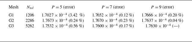
 P
 Re=55.1
 g=1
 P=9
 ω=0.6419

 g

 σ
 kz
 Rec=303.4
 g=0.2
 55.1
 g=1
 22.8
 g=1.8


 Re=58
 g=1
 (a)
 Cl
 (b)
 Cl
 σ=0.01497
 (c)
 β=0.05367

 σ
 α
 g=1
 g=0.4

 Open access

