





1. Introduction
High-speed-vehicle design requires the consideration of many fundamental fluid-mechanic phenomena (Leyva Reference Leyva2017). Impacts with drops or small particles at high velocity can degrade aerospace materials, reducing transparency and other desirable properties (Lapp, Stutzman & Wahl Reference Lapp, Stutzman and Wahl1954; Jenkins Reference Jenkins1966; Reinecke Reference Reinecke1974; Schmitt Reference Schmitt1975; Smith Reference Smith1976; Callens & Lawrence Reference Callens and Lawrence1981; Gohardani Reference Gohardani2011; Moylan, Landrum & Russell Reference Moylan, Landrum and Russell2013). The sphericity and size of a drop can change the degree of damage upon impact (Adler Reference Adler1975; Adler & Hooker Reference Adler and Hooker1978; Adler Reference Adler1982, Reference Adler1987, Reference Adler1995a,Reference Adlerb, Reference Adler1999; Lee et al. Reference Lee, Park, Farid and Yoon2012). Additionally, the flow structure about a high-speed vehicle, namely the leading shock wave, can disrupt a drop, potentially altering the deleterious effects of impact (Engel Reference Engel1958; Nicholson Reference Nicholson1967; Ranger & Nicholls Reference Ranger and Nicholls1969, Reference Ranger and Nicholls1972; Reinecke & McKay Reference Reinecke and McKay1969; Waldman & Reinecke Reference Waldman and Reinecke1971; Simpkins & Bales Reference Simpkins and Bales1972; Waldman, Reinecke & Glenn Reference Waldman, Reinecke and Glenn1972; Barber et al. Reference Barber, Taylor, Grood and Hopkins1975; Reinecke & Waldman Reference Reinecke and Waldman1975; Barber Reference Barber1976). Numerous researchers have devised drop breakup models, such as the Taylor analogy breakup (TAB) model from O'Rourke & Amsden (Reference O'Rourke and Amsden1987). Researchers have added to these breakup models (Beale & Reitz Reference Beale and Reitz1999; Schmehl Reference Schmehl2002; Stefanitsis et al. Reference Stefanitsis, Strotos, Nikolopoulos, Kakaras and Gavaises2019), and, more recently, have worked towards integrating these models in high-speed, multidimensional flow (Hess et al. Reference Hess, Kessler, Johnson, Goodwin, Aguilera and Sosa2021; Aguilera et al. Reference Aguilera, Sosa, Hyde, Goodwin, Hess and Kessler2023; Daniel et al. Reference Daniel, Guildenbecher, Delgado, White, Reardon, Stauffacher III and Beresh2023).
The first phase of this problem is processing of the drop by a bow shock, the strength of which is determined by the Mach number of the projectile (here,  $M_p>3$). The drop begins the aerobreakup process post-shock in a non-constant flow, juxtaposed to the near-constant flow in drop demise experiments in a shock tube. Then, the altered drop impacts a surface at hypervelocity, which results in a complex multiphase flow field. Major dimensionless groups that govern aerobreakup and drop impact that have been identified include the Weber number, the Reynolds number, the Ohnesorge number, the Mach number and the Knudsen number. The Weber number is the ratio of the aerodynamic force to the restoring capillary force on the drop and can be written as
 \begin{equation} We_A = \frac{\rho_g U_A^{2} d_{d}}{\sigma}.\end{equation}
Here,  $\rho _g$,
 $U_A$,
 $d_d$ and
 $\sigma$ are, respectively, the local gas density, the velocity difference between the local gas and the drop, the drop diameter and the surface tension for the drop–gas interface. The drop impact and aerobreakup research communities often use different values for density and velocity in this calculation. The Reynolds number is the ratio of the inertial to the viscous forces and can be written as
 \begin{equation} Re_A = \frac{\rho_g U_A d_{d}}{\mu_g}.\end{equation}
Here,  $\mu _g$ is the dynamic viscosity of the local gas. The Ohnesorge number relates viscous forces to the inertial and surface-tension forces as
 \begin{equation} Oh = \frac{\mu_{d}}{\sqrt{\rho_{d} d_{d} \sigma}} ,\end{equation}
noting the impact and aerobreakup communities write it the same way and that, here,  $\rho _d$ and
 $\mu _d$ refer to the liquid drop density and viscosity. The Mach number is velocity relative to the local sound speed as
 \begin{equation} M_A = \frac{U_A}{a_g} = \frac{U_A}{\sqrt{\gamma_g R_g T_g}},\end{equation}
where  $a_g$,
 $\gamma _g$,
 $R_g$ and
 $T_g$ are the sound speed, ratio of specific heats, the gas constant and the temperature of the local gas, respectively.
The time,  $t$, since interaction with the bow shock of the projectile is typically non-dimensionalized by the so-called ‘characteristic breakup time’ (Ranger & Nicholls Reference Ranger and Nicholls1969; Reinecke & McKay Reference Reinecke and McKay1969) or ‘Rayleigh time’ (Hébert et al. Reference Hébert, Rullier, Chevalier, Bertron, Lescoute, Virot and El-Rabii2020),
 \begin{equation} t_{C2} = \sqrt{\frac{\rho_d}{\rho_{g2}}} \frac{ d_{d} }{ U_{2LF} },\end{equation}
as  $\tau = t/t_{C2}$. Here, the conditions immediately behind the bow shock of the projectile are chosen to define the characteristic time so that comparisons are consistent with the literature.
The first part of the problem of high-speed-vehicle/rain encounter is drop aerobreakup, which will be the focus of this paper. Work on the impact portion of this problem will be left to a follow-on paper. Aerobreakup is often characterized by different breakup regimes corresponding to increasing aerodynamic force on the liquid drop (Hinze Reference Hinze1949a,Reference Hinzeb, Reference Hinze1955; Lane Reference Lane1951; Pilch & Erdman Reference Pilch and Erdman1987; Hsiang & Faeth Reference Hsiang and Faeth1995). As the ratio of aerodynamic force to restoring capillary force on the drop increases (non-dimensionalized as the Weber number,  $We_A$), the drop is said to pass through different breakup regimes. At low Weber numbers (
 $We_A < 100$), the drop is said to pass from a vibrational breakup regime through the bag breakup regime to the bag-and-stamen breakup regime and then the multimode breakup regime (Pilch & Erdman Reference Pilch and Erdman1987).
Above  $We_A \approx 350$, there exists controversy in the literature on what the breakup mechanism is. Additionally, there is uncertainty on what value of
 $We_A$ for which there exists, if any, a high-Weber-number regime, whereby the Weber number no longer delineates breakup mechanisms. Pilch & Erdman (Reference Pilch and Erdman1987) propose that, at higher Weber numbers, the drop enters a sheet-stripping regime (
 $100 \lessapprox We_{A} \lessapprox 350$), a wave-crest stripping regime (
 $We_{A} \gtrapprox 350$) and then a regime they term ‘catastrophic’ also for
 $We_{A} \gtrapprox 350$. The ‘catastrophic’ regime is characterized by relatively long-wavelength surface instabilities that grow in amplitude until they are comparable to the drop diameter, at which point the drop breaks into smaller droplets. This can occur before wave-crest stripping can completely reduce the drop mass.
Theofanous, Li & Dinh (Reference Theofanous, Li and Dinh2004), Theofanous et al. (Reference Theofanous, Li, Dinh and Chang2007, Reference Theofanous, Mitkin, Ng, Chang, Deng and Sushchikh2012) and Theofanous (Reference Theofanous2011) propose a different understanding of drop demise. In their model, Rayleigh–Taylor (RT) surface instability dominates initially at higher ( $We_{A} \approx 1\times 10^2$) Weber numbers. In the RT-dominated regime (dubbed RT piercing, or RTP), surface waves are comparable in amplitude to the drop diameter. Starting from
 $We_A \approx 1\times 10^2\unicode{x2013}1\times 10^3$, and as
 $We_A$ becomes large, the regime transitions to shear-induced entrainment (SIE), where mass is stripped from the drop. Several researchers have performed research at Weber numbers in the regime where RTP is expected to transition to SIE. Wierzba & Takayama (Reference Wierzba and Takayama1988) experimentally studied aerobreakup at
 $We_A = 600\unicode{x2013}7600$ with holography and presented a four-stage stripping-type mechanism. Chou, Hsiang & Faeth (Reference Chou, Hsiang and Faeth1997) studied experimentally the temporal properties of drop breakup in the shear breakup for
 $We_A=125\unicode{x2013}375$. Dorschner et al. (Reference Dorschner, Biasiori-Poulanges, Schmidmayer, El-Rabii and Colonius2020) studied numerically and experimentally the formation and recurrent shedding of ligaments in drop aerobreakup in this transitional regime. The introduction of that paper gives a good review of the different breakup regimes and asserts that the ligament formation process in the vicinity of the RTP–SIE transition and beyond (i.e.
 $We_A >1\times 10^2$) is a subject of current investigation (Jalaal & Mehravaran Reference Jalaal and Mehravaran2014; Meng & Colonius Reference Meng and Colonius2015, Reference Meng and Colonius2018; Jain et al. Reference Jain, Tyagi, Prakash, Ravikrishna and Tomar2019; Wang et al. Reference Wang, Hopfes, Giglmaier and Adams2020). Theofanous & Li (Reference Theofanous and Li2008) used laser-induced fluorescence to image the aerobreakup of drops in Mach 3 flow at Weber numbers up to
 $5.4\times 10^3$. The liquid was tributylphosphate (TBP), which those researchers call ‘water-like’, given it is Newtonian, has a higher viscosity than water (4 mPa s) and lower surface tension (27.3 mN m
 $^{-1}$) at room temperature. Those researchers assert that previous research performed with shadowgraphy ‘allowed misinterpretations that have led to inappropriate conceptualizations (and theory) of the physics that govern breakup at high Weber numbers’. Continuing, ‘for
 $We_A>1\times 10^3$, breakup occurs by SIE, which is a regime dominated by shear (and damping of RT waves due to shear-induced straining) and one that is mechanistically different from (the previously hypothesized) stripping’. The researchers also discuss potential phase change and surface-tension reduction in high-temperature experiments. Theofanous et al. (Reference Theofanous, Mitkin, Ng, Chang, Deng and Sushchikh2012) studied water drops at shock Mach numbers
 $M_s=1.1\unicode{x2013}2.1$ and
 $We_A=60-3\times 10^4$. They also studied TBP at
 $M_s=1.02\unicode{x2013}2.5$ and
 $We_A=12\unicode{x2013}1.5\times 10^5$. The results of that work lead the authors to assert that SIE is the ‘second and terminal criticality’. Theofanous (Reference Theofanous2011) provides a complete review of aerobreakup, discussing the relevant non-dimensional numbers pertinent to Newtonian and viscoelastic fluids. In that review, § 4.2 titled ‘Shear-Induced Entrainment is the Terminal Regime’ discusses how the ‘so-called catastrophic regime, thought to exist for Weber numbers greater than
 $\approx 1\times 10^3$, was an artifact of shadowgraphs’. They then suggest that, for increasing Weber number, SIE is increasingly favoured over RTP.
More closely related to this paper is research at high Weber ( $We_{A} > 1\times 10^4$) and Mach number (
 $M_s>3$). Ranger & Nicholls (Reference Ranger and Nicholls1969, Reference Ranger and Nicholls1972) studied drop demise in a shock tube at shock Mach number 1.5–3.5, in atmospheric air, yielding Weber numbers above
 $1\times 10^4$. Notably, those researchers devised the ‘characteristic breakup time’ and proposed a detailed model of boundary-layer stripping, noting that ‘[t]he shearing action exerted by the high-speed flow causes a boundary layer to be formed in the surface of the liquid and the stripping away of this layer accounts for the breakup’. This is likely among the first times SIE was recognized as a drop-demise mechanism.
Reinecke & McKay (Reference Reinecke and McKay1969) studied water drop breakup behind Mach 3–12 shocks at relatively high pressure, 90–760 torr, yielding results with Weber numbers greater than  $1\times 10^4$. They found that ‘at shock speeds from Mach 3 to Mach 6 the drops are progressively stripped by the shearing of the surrounding air
 $\ldots$ Above Mach 6, where the drops experience accelerations in excess of
 $1\times 10^6$ g, an apparent surface instability results in the destruction of the drop before breakup is accomplished by the stripping action’.
Krauss (Reference Krauss1970) studied water drop displacement and flattening behind Mach 1.6–3 shocks in a shock tube. A stream of liquid drops of diameter 0.5 to 3.2 mm was injected into a test section at 1 atmosphere, yielding aerobreakup Weber numbers in the range  $1.3\times 10^3$ to
 $1.2\times 10^5$. Jaffe (Reference Jaffe1975) performed similar work, studying drop displacement and flattening behind Mach 7.5–13.9 shocks in the NASA EAST shock tube with initial pressure of 0.13–0.50 atm, yielding Weber numbers greater than
 $1\times 10^5$.
In their review of the literature, Pilch, Erdman & Reynolds (Reference Pilch, Erdman and Reynolds1981) referred to Ranger & Nicholls (Reference Ranger and Nicholls1969) and Ranger & Nicholls (Reference Ranger and Nicholls1972) and their analysis of boundary-layer stripping. He computes the time required for the boundary-layer stripping process to reduce the mass of a liquid drop to zero and compares that calculated time with the measured drop-demise time found by Engel (Reference Engel1958) and Ranger & Nicholls (Reference Ranger and Nicholls1969). He concludes that the required time for drop demise due to boundary-layer stripping alone is up to an order of magnitude greater than the observed demise time. He concludes that boundary-layer stripping cannot then be the sole mechanism of drop aerobreakup, and that a breakup mechanism driven by surface instability must also be present.
Boiko, Papyrin & Poplavskii (Reference Boiko, Papyrin and Poplavskii1987) studied the interaction of drops at an initial pressure of 20–100 kPa with a shock wave at Mach numbers  $M_s = 2\unicode{x2013}6$ and Weber numbers in the range
 $1\times 10^4\unicode{x2013}1.3\times 10^5$. Those researchers tracked the drop movement. They also assert that a ‘major role in disintegration of low viscosity liquids [referring to water] in a shock wave with
 $M_s = 2\unicode{x2013}4$ is played by the mechanism of removal of a surface layer of liquid, which acts after an induction period
 $t_i$ and continues through the complete decay of the droplet’.
Joseph, Belanger & Beavers (Reference Joseph, Belanger and Beavers1999) studied drop demise in a shock tube at shock Mach number 2–4 with pre-shocked air pressures of 50–58 kPa, yielding Weber numbers in the range  $4\times 10^4\unicode{x2013}1.6\times 10^5$ for drops of water in addition to several other liquids. ‘The thesis of [that] paper is that breakup at high accelerations, corresponding to high Weber numbers, is controlled at early times by Rayleigh–Taylor instabilities’. Joseph, Beavers & Funada (Reference Joseph, Beavers and Funada2002) continued that work for Newtonian and viscoelastic fluids. Joseph et al. (Reference Joseph, Belanger and Beavers1999, Reference Joseph, Beavers and Funada2002) both provide a detailed stability analysis to support their assertions based on experimental data.
Hébert et al. (Reference Hébert, Rullier, Chevalier, Bertron, Lescoute, Virot and El-Rabii2020) studied aerobreakup experimentally and numerically at Mach 4.4 and Weber numbers above  $1\times 10^5$, which overlaps the parameter space of the work presented in this paper. In that work, they report on the drop displacement and flow morphology during three breakup steps delineated by non-dimensional breakup time. The drops were suspended at the crossing of two 25
 $\mathrm {\mu }$m copper wires by capillary force. Virot et al. (Reference Virot, Tymen, Hébert, Rullier and Lescoute2023) used a similar strategy to study aerobreakup at Mach numbers 4.3 and 10.6 for long non-dimensional breakup time at Weber numbers
 $5\times 10^4\unicode{x2013}1.1\times 10^5$. The authors make comments on heat transfer and the mist formation at the differing Mach numbers.
Salauddin et al. (Reference Salauddin, Morales, Hytovick, Burke, Malik, Patten, Schroeder and Ahmed2023) images the breakup of liquid rocket propellant drops at  $M_s=5.1$ and
 $We_A=1.2\times 10^5$ in a detonation facility. They argue that the ‘transition from a shock wave to a detonation suppresses the deformation of the droplet and augments small-scale breakup’. They go on to discuss that, at high Weber and Mach numbers, ligaments are generated and finally, a ‘jellyfish’ structure is formed during the drop breakup process.
This review of the current literature identifies a dearth of high-quality aerobreakup data at high Mach, Weber and Reynolds numbers. Moreover, much of the research in the literature was performed with a shock tube, where there is a well-defined, impulsive start to the flow. In the present work, new experimental data and computations are presented on aerobreakup at high Mach and Weber numbers in the stagnation region of high-speed flow over a bluff body.
Additionally, a long-standing discrepancy in the literature is identified where some researchers assert that linear instability growth results in rapid and sudden drop breakup when the instability amplitude becomes comparable to the drop thickness (Reinecke & McKay Reference Reinecke and McKay1969; Joseph et al. Reference Joseph, Belanger and Beavers1999). Others, including Theofanous & Li (Reference Theofanous and Li2008) and Theofanous (Reference Theofanous2011), assert that this is incorrect and that drop breakup is governed exclusively by mass stripping. The present work develops a model for surface instabilities based on linear-stability theory from Funada & Joseph (Reference Funada and Joseph2001) and shows a mismatch between the predicted amplitude and wavelength from that model and those observed in either shadowgraph images or numerical simulations. A model for nonlinear growth from Pilch et al. (Reference Pilch, Erdman and Reynolds1981) was used for large instability amplitudes and further developed; agreement between this model and computations is good.
2. Facility and experimental set-up
The experiments were performed at the Naval Surface Warfare Center Dahlgren Division's electromagnetic launcher (EML) located at the Hypersonic Integration and Test (HIT) facility at the Potomac River Test Range located in Dahlgren, Virginia, USA (Tadjdeh Reference Tadjdeh2017). The EML digitally prescribes projectile launch acceleration profiles so it provides a ground-test capability with a broad range of precisely controlled velocities for weather encounters and terminal impacts with a launch cadence of multiple shots per day (O'Rourke Reference O'Rourke2017). For this testing campaign, eight bore-rider projectiles were fired at velocities between 1000 and 1800 m s $^{-1}$ into a sea-level atmosphere. The flat-faced, bore-rider projectiles were approximately rectangular and 100 mm wide
 $\times$ 150 mm tall. Water drops of diameter from 0.51–2.30 mm were suspended along the projectile's line of flight using acoustic levitators (Marzo, Barnes & Drinkwater Reference Marzo, Barnes and Drinkwater2017; Sheldon Reference Sheldon2019), noting that the use of acoustic levitation in shock tubes has been done before by, for example, Hanson, Domich & Adams (Reference Hanson, Domich and Adams1963) and Dorschner et al. (Reference Dorschner, Biasiori-Poulanges, Schmidmayer, El-Rabii and Colonius2020). Acoustic levitators were chosen for this application instead of suspending the drops from wire, as in Hébert et al. (Reference Hébert, Rullier, Chevalier, Bertron, Lescoute, Virot and El-Rabii2020), or releasing the drops from a dripper, as in many other works. This is because levitators made it easier to hold drops in the small field of view in the camera's relatively narrow depth of field. The levitators did not observably disturb the drop surfaces; pressure waves from levitator transmitters are not present in shadowgraphs and there is no observable distortion of the projectile bow shock or on the drop surface before the projectile arrives.
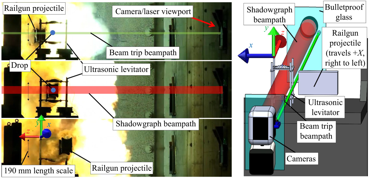
In figure 1, three frames of high-speed video looking uprange toward the rail-gun muzzle are presented along with a schematic of the experimental set-up. A coordinate system is placed in each to orient the reader. The projectile can be seen passing through the acoustic levitator frame before, during and after interaction with the drop. In figure 1-top, before the interaction, a green laser beam that acts as a ‘tripwire’ to initiate the high-speed cameras can be seen as a semitransparent green line. In figure 1-middle, during the interaction, a high-speed laser light source, seen as a semitransparent red line, is initiated and synchronized to a high-speed camera. Finally, in figure 1-bottom, after the interaction, the high-speed projectile is seen having passed cleanly through the levitator frame.
Three frames looking uprange toward the rail-gun muzzle. The approximately rectangular (100 mm wide  $\times$ 150 mm tall) projectile is seen traversing the flight path through the levitator. The three frames depict periods before the imaging system is triggered by the ‘beam trip’, during shadowgraph recording, and after the projectile has traversed the field of view. Cartoons of drop and laser beams are not to scale. For additional context, a movie of this projectile flying through the levitator is provided as supplementary movie 7 available at https://doi.org/10.1017/jfm.2024.1092.
Back-lit shadowgraphy and front-lit imaging were used to image the drop (Hauser et al. Reference Hauser, Edgerton, Holt and Cox1936; Settles Reference Settles2001; Danehy et al. Reference Danehy, Weisberger, Johansen, Reese, Fahringer, Parziale, Dedic, Estevadeordal and Cruden2018). For the back-lit shadowgraphy, the drop–projectile interaction is illuminated from behind by a laser light source synchronized to a Kirana high-speed camera operated at 2–4 million frames per second (f.p.s.) with 100 ns exposure. The lens used on the Kirana was a AF-S NIKKOR 200 mm f/2G ED-VR-II positioned approximately 2.8 m from the drop behind 50 mm of bulletproof glass. To achieve approximately 20 pixels mm $^{-1}$ resolution, one
 $2\times$ teleconverter, one
 $1.4\times$ teleconverter and 92 mm of lens tube were placed between the lens and the camera body. The experiment was designed such that an object moving at 500 m s
 $^{-1}$ would be imaged with one pixel of image blur. A bandpass filter at the laser wavelength was placed in the lens tube to attenuate muzzle flash to mitigate oversaturation. For the front-lit imaging, a Phantom TMX 7510 camera was run at 300k f.p.s., with a 190 ns exposure time; the light source was the rail-gun muzzle flash. A Sigma 150–600 mm f/5–6.3 was used with one
 $2\times$ and one
 $1.4\times$ teleconverter to provide 11.5 pixels mm
 $^{-1}$ resolution. The front-lit imaging did not yield useful data for this experimental campaign. The projectile interrupts a 532 nm laser beam, which is pointed at a DET36A2 biased photodetector with an FL532 bandpass filter. When that beam is interrupted, the falling edge signal from the photodetector triggers an oscilloscope's output, which triggers a pulse generator, in turn triggering the high-speed cameras.
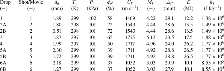
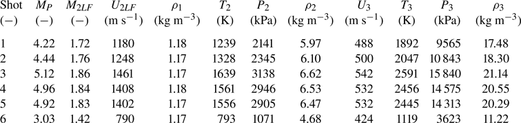
The ambient and launch conditions of the six shots are reported in table 1. Here,  $d_{d}$,
 $T_{1}$,
 $P_{1}$ and
 $\phi _{R}$ are the drop diameter, the ambient temperature and pressure and the relative humidity, respectively. Also,
 $U_{P}$,
 $M_{P}$,
 $\varDelta _{P}$,
 $E$ and
 $h_{T}$ are the projectile velocity, projectile Mach number, shock standoff distance, the programmed launch energy of the EML and total enthalpy of the flow, respectively.
Dahlgren shot conditions.
3. Stagnation point flow model
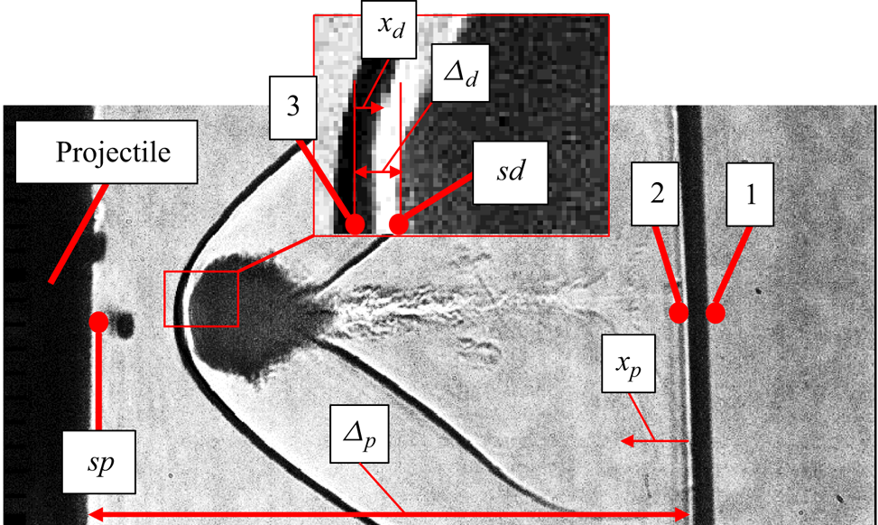
In this section, a simple model is devised to find the flow parameters (e.g. Weber or Reynolds number) that define the problem of aerobreakup along the stagnation streamline of a bluff body in high-speed flow. This model enables the quick and clear definition of the problem and parameter space so that the relevancy of phenomena and appropriateness of assumptions may be assessed (e.g. calorically perfect gas, vibrational relaxation, thermochemistry, humidity, etc.). Here, it is assumed the drop is processed by the projectile bow shock and then by the gas along the stagnation streamline of the projectile; also, the drop does not disturb the mean flow. Further, a one-dimensional, reacting gas dynamics model, where the mass flux linearly decreases from the point behind the bow shock to zero at the corresponding stagnation point, is assumed to adequately capture the major characteristics of the flow, given the drops are much smaller than the projectile size ( $>50\,:\,1$). The different states of the flow are marked in figure 2. This stagnation point problem is solved twice for each case, first for the projectile along
 $x_p$ from state 2 to state
 $sp$, and then for the drop itself along
 $x_d$ from state 3 to state
 $sd$. The calculations to predict the flow along the stagnation streamline were performed with Cantera (Goodwin Reference Goodwin2003; Goodwin et al. Reference Goodwin, Moffat, Schoegl, Speth and Weber2022) using the shock and detonation toolbox (SDT) (Browne et al. Reference Browne, Ziegler, Bitter, Schmidt, Lawson and Shepherd2018) in MATLAB. Technical details of the calculations and some nomenclature are in Appendix A.
Definition of the different states. Here, 1, 2 and  $sp$ mark the ambient state (table 1), the post-bow shock state and the stagnation point on the projectile, respectively. The parameters
 $\varDelta _p$ and
 $x_p$ are the projectile bow shock standoff distance and the coordinate along the stagnation streamline from 2 to
 $sp$, respectively; 3 and
 $sd$ are the post-bow shock state of the drop and the stagnation state of the drop, respectively. Finally,
 $\varDelta _d$ and
 $x_d$ are the drop bow shock standoff distance and the coordinate along the stagnation streamline from 3 to
 $sd$, respectively.
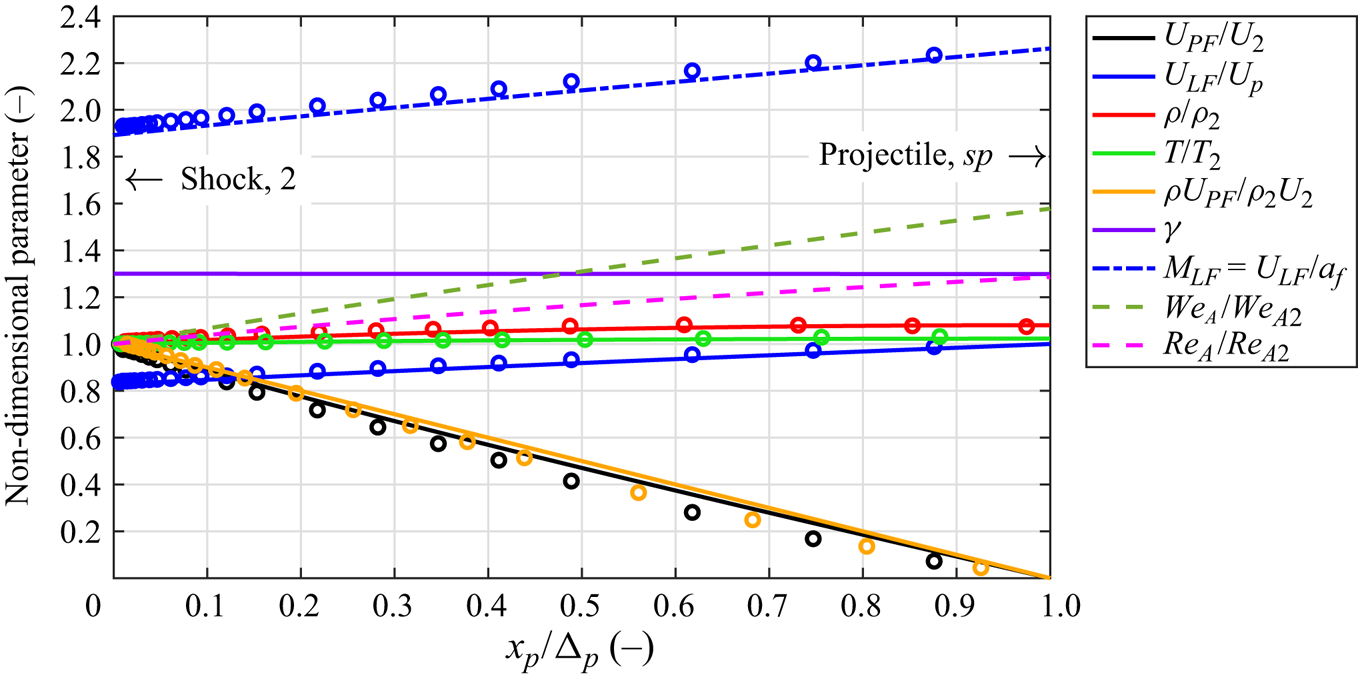
Relevant post-shock quantities are non-dimensionalized and presented in figure 3. Here, a linearly decreasing mass flux is shown, per the model, along with a decreasing velocity in the projectile frame,  $U_{PF}/U_2$. The gas velocity that the drop experiences is that in the laboratory frame; that is,
 $U_A$ from (1.1) is
 $U_{LF}/Up$. That the velocity experienced by the drop increases from the post-shock state to the velocity of the projectile is an illustration of the importance of considering the reference frame. The post-shock Mach number is supersonic in the laboratory frame, increasing from 1.9 to over 2.2. The thermodynamic parameters do not change much in the stagnation region of the projectile, namely the temperature (
 $<2$ %), density (
 $<8$ %) and ratio of specific heats (
 $<1$ %). This is in part because the enthalpy of these shots is not high enough to induce substantive chemical reaction. Using the definition of the Knudsen number from Loth (Reference Loth2008), it was determined that all experiments were executed in the continuum regime. Importantly, the ratio of specific heats is observed to be constant and
 $\gamma \approx 1.3$. The aerobreakup Weber number,
 $We_A$, and Reynolds number,
 $Re_A$, increase by
 ${\approx }50\,\%$ and
 ${\approx }25\,\%$, respectively. Although these increases are appreciable, they most likely do not alter the drop-breakup regime. Additionally,
 $We_A = \rho _g U_{LF}^{2} d_{d} / \sigma$, so it essentially parameterizes the aerodynamic pressure on the drop; that is, the aerodynamic pressure increases
 ${\approx }50\,\%$.
Non-dimensional quantities for the solution along the stagnation streamline for shot 3. Here, lines are from the thermicity model and the dots represent the simulations detailed in § 4.
A similar solution procedure is used to calculate the conditions behind the bow shock of the drop, a compression from state 3 to a hypothetical stagnation point on the drop, state  $sp$ (figure 2). The initial conditions are derived from the jump conditions; however, state 1 is replaced with values computed along the stagnation streamline, and state 2 becomes state 3. The case where the drop is half-way along the stagnation streamline,
 $x_p = \varDelta _p/2$, is highlighted. The solution is presented in figure 4 with non-dimensional quantities and mole fractions. Some chemical non-equilibrium is apparent, as up to 4 % NO is being produced at a hypothetical stagnation point on the drop face. The ratio of specific heats is nearly constant,
 $\gamma \approx 1.28$.
Non-dimensional quantities (a) and mole fractions (b) along the stagnation streamline from behind the bow shock of the drop to the drop face. Here, lines are from the thermicity model and the dots represent the simulations detailed in § 4.

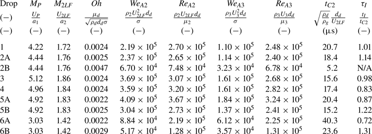
Dimensional and non-dimensional conditions at the post-shock states 2 and 3 are summarized in tables 2 and 3, respectively. Aerobreakup Weber/Reynolds numbers at state 3 are reported because these are the conditions to which the drop is exposed. This is analogous to boundary-layer studies on high-speed bodies referencing the Mach/Reynolds number at the boundary-layer edge, not the free-stream Mach/Reynolds number. Because the jump condition for mass dictates that the product of  $\rho U$ is constant and the dynamic viscosity will go up due to higher temperature in state 3,
 $Re_{A2}$ is similar to
 $Re_{A3}$. The Weber numbers corresponding to state 3 are approximately 30 %–60 % of that in state 2. As such, it is asserted that the non-dimensional numbers at state 2 offer a sufficient point of comparison with other aerobreakup research at high Weber and Reynolds numbers because the values do not change enough as the drop traverses the stagnation streamline to change the aerobreakup regime. Additionally, the gas in the stagnation region of the projectile at these conditions can be approximated as a calorically perfect gas with a ratio of specific heats of
 $\gamma \approx 1.3$. This assumption was used to complete the detailed simulations in § 4.
Dimensional conditions in states 1, 2 and 3.
Non-dimensional parameters for the current test campaign.
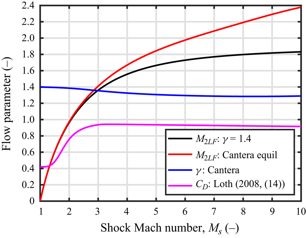
The drop is subject to supersonic flow in the laboratory frame for all cases presented in this work. In figure 5, the shock Mach number,  $M_s$, is plotted against the Mach number of the drop in the laboratory frame for a perfect gas and a gas in thermochemical equilibrium. For M
 $_s\approx 2$, the drop will be in transonic flow in the laboratory frame. Much research in this area is performed in facilities with M
 $_s\approx 2$. To highlight the effect on the flow field, (14) from Loth (Reference Loth2008) is used to plot the drag coefficient for a sphere using
 $M_{2LF}$ as the input. All of the conditions in this work are at projectile Mach numbers of at least
 $M_P=M_s=3$, so the Mach number in the laboratory frame for this work is not transonic, as
 $M_{2LF}>1.4$.
Shock number,  $M_s$, vs post-shock Mach number in the laboratory frame,
 $M_{2LF}$, for a perfect gas with
 $\gamma =1.4$ and in chemical equilibrium. Ratio of specific heats as computed by Cantera,
 $\gamma$, and
 $C_D$ as computed with (14) of Loth (Reference Loth2008) for
 $M_{2LF}$.
The calorically perfect gas assumption is sometimes not appropriately applied in the high-speed aerobreakup literature. The calculations done by Theofanous & Li (Reference Theofanous and Li2008) in their tables I and II while discussing the work of Reinecke & McKay (Reference Reinecke and McKay1969) do not account for thermochemistry. Those calculations are performed assuming a calorically perfect gas with the ratio of specific heats set to 1.4 and predict temperatures that are too high, and the resulting assertions that are made may not be correct. Accounting for thermochemistry in those calculations would reduce the post-shock temperature considerably (Thompson Reference Thompson1988; Anderson Reference Anderson2011). It is imperative that the often-used calorically perfect gas assumption with the ratio of specific heats set to 1.4 be evaluated for shock Mach numbers exceeding 3, with or without a projectile. The post-shock thermodynamic parameters ( $P, T, \rho$) can be incorrectly predicted, which can change basic flow features, such as the shock standoff distance of the drop.
4. Numerical simulation set-up
This computational study utilizes the Allaire, Clerc & Kokh (Reference Allaire, Clerc and Kokh2002) viscous five-equation model, which encompasses two equations dedicated to mass conservation of the liquid and gas phases, momentum equations for each spatial direction, an energy equation and a non-conservative volume-fraction advection equation. The complete governing equations can be found in Appendix B.
The Allaire model has been used in previous aerobreakup and shock–drop interaction works (Meng & Colonius Reference Meng and Colonius2018) due to its ability to suppress pressure oscillations at material interfaces (Abgrall Reference Abgrall1996). The model was designed to characterize immiscible fluids, and so, the interfacial region is subjected to artificial mixing due to resolution constraints and missing surface tension. Nevertheless, comparison with experiments, at least for the high-Mach-number conditions considered in this work, seems to build confidence in the ability of the model to capture the major instability mechanisms in the front face, as well as the evolution of the mist boundaries (see figure 18 in § 8.3).
The governing equations are solved with a fifth-order weighted compact nonlinear scheme adapted from Wong et al. (Reference Wong, Angel, Barad and Kiris2021) which employs higher-order flux and variable reconstruction, as well as a positivity-preserving limiting procedure switching to a first-order Harten–Lax–van Leer contact Riemann solver to ensure robustness. The viscous terms are discretized using regular centred second-order accurate conservative finite difference discretization. For time integration, a third-order strong stability-preserving Runge–Kutta method is employed. The numerical simulation approach was previously validated in several works (Viqueira-Moreira et al. Reference Viqueira-Moreira, Stoffel, Poovathingal and Brehm2022; Stoffel et al. Reference Stoffel, Viqueira-Moreira, Brehm and Poovathingal2023; Viqueira-Moreira et al. Reference Viqueira-Moreira, Dworzanczyk, Parziale and Brehm2023a,Reference Viqueira-Moreira, Gonuleri, Leigh, Watson, Guven and Brehmb).
For the current simulations, the projectile with a rectangular cross-section is immersed in the flow domain using an established immersed boundary method (Brehm, Hader & Fasel Reference Brehm, Hader and Fasel2015; Brehm, Barad & Kiris Reference Brehm, Barad and Kiris2019; Boustani et al. Reference Boustani, Barad, Kiris and Brehm2021). Firstly, a perfect gas base flow is computed to establish a flow field around the projectile. Secondly, a drop is inserted in front of the shock front convecting with the mean flow. For computational efficiency, adaptive mesh refinement (AMR) is used, tracking the pressure gradient to follow the shock front and the water volume fraction to track the drop. A total of 12 refinement levels are used to be able to provide sufficient grid resolution around the drop to maintain at least 150 grid points per diameter. A schematic of the simulation set-up is shown in figure 6(a), the flow field around the projectile in figure 6(b) and an overview of the AMR grid topology with colour contours of  $u$-velocity contours in figure 6(c).
Schematic showing adaptive mesh refinement tracking of the drop.

5. Overview of results and discussion
5.1. Overview of experimental results
The high-speed movies from each of the cases are included as supplementary material and are numbered according to the shot they depict. Supplementary movie 1 shows the first successful experiment, illustrating that aerobreakup and impact can be visualized in the unique environment of an outdoor rail-gun facility. Supplementary movie 2 shows two drops in the same stagnation region. Here, the importance of the characteristic breakup time,  $t_{C2}$, is seen as the smaller of the two drops breaks up appreciably earlier and does not impact the projectile. Supplementary movies 3–5 were recorded with nominally matching conditions, enabling the study of different sized drops (thus, different Weber and Reynolds numbers) at projectile Mach number
 $M_P=5 +0.12/-0.08$. Supplementary movie 6 was recorded with
 $M_P=3.03$ to overlap with previous shock tube aerobreakup studies and complete the parameter space as best possible at the time. Two drops are seen in the stagnation region, the smaller of which appears to break up before impact. Finally, video of the projectile flying through the levitator is provided as supplementary movie 7.
Hereafter, the results from the drop 3 experiment (supplementary movie 3) and the drop 4 experiment (supplementary movie 4), which are at nominally matching conditions, are compared with the results from the drop 6B experiment (supplementary movie 6). These cases are compared because they highlight distinct differences in the flow topology observed at noticeably different Mach and Weber numbers. The naming convention of each drop follows tables 1 and 3. Four sample shadowgraph images from the drop 3 experiment are shown in figure 7 to give the reader an idea about the finer flow features that could be captured in the experiments.
Four shadowgraphs of the high-speed movie for drop 3 showing the shock structure about the drop. Short red ticks denote millimetre increments. Long red ticks denote centimetre increments. Full movie included as supplementary movie 3.

5.2. Overview of computational results and discussion
Figure 8 gives an overview of the aerobreakup process as observed in the simulations. Drops 3 (Mach 5 case) and 6B (Mach 3 case) display similar overall dynamics, but some key differences are observed and will be analysed hereafter. As the drop enters the shock layer (shock structure is discussed in detail in § 6), the aerobreakup process begins, causing a substantial change to the drop shape. Different colour schemes were chosen for velocity contours in figure 8 for inside, outside and the wake of the drop, as the velocity scales in these regions of the flow domain are widely different. Firstly, the drop experiences a strong, non-spatially uniform deceleration due to compressibility effects. The front of the drop experiences much larger acceleration than the back, causing flattening. The flattening of the back of the drop shape has been discussed in prior work. For example, Meng & Colonius (Reference Meng and Colonius2018) note that high pressures at the forward and rear stagnation points contribute to the flattening. In the present simulations, the pressure at the front face is the main driver of this ‘pancaking’, with much lower pressures at the rear. Negative pressures can be observed inside the drop, meaning it undergoes internal tension (Azouzi et al. Reference Azouzi, Ramboz, Lenain and Caupin2012; Caupin et al. Reference Caupin, Arvengas, Davitt, Azouzi, Shmulovich, Ramboz, Sessoms and Stroock2012). This is modelled through the stiffened gas equation of state (see Appendix B). Although cavitation effects could play a role in the flow field evolution, they are disregarded in this study. Additionally, the computations predict that the aspect ratio of the liquid mass of the drop changes appreciably with time. That is, mass is shed from the windward drop face while the aerodynamic forces flatten the drop, accentuating this increase in aspect ratio. Figure 8 shows that the liquid drop has an aspect ratio of  $b/c\approx 1, 2, 4$ (spanwise vertical,
 $y$ to streamwise,
 $z$) at times
 $\tau \approx 0.25, 0.50, 0.75$, respectively. Drop displacement and flattening are discussed in detail in § 7. The wake dynamics is distinct in figure 8, with the wake of drop 6B becoming turbulent sooner than that of drop 3. Instability at the windward gas/liquid interface is readily apparent in figure 8. The presence of the RT and Kelvin–Helmholtz (KH) instabilities can be seen in the 0.1-volume-fraction contour lines where RT seems to dominate the front centre region of the drop, and the KH instability becomes more apparent closer towards the equator. Once the drops have substantially flattened, strong bursting events can be observed, e.g. for drop 3 at
 $\tau =1.0$. Both drops are close to catastrophic breakup at
 $\tau =1.0$, displaying drop surface waviness amplitudes reaching the thickness of the drop. With increasing simulation time, the dominant wavelength of the deformed gas–liquid interface is increasing; e.g. compare snapshots
 $\tau =0.25$ and
 $\tau =1.0$. These characteristics will be investigated further with linear- and nonlinear-stability analyses in § 8.
Velocity and pressure contours in centre cut plane for drops 3 (a) and 6B (b) at four different times. Note different colour maps correspond to different ranges for inside the drop, outside the drop and in the wake.

Before discussing further details of the aerobreakup process observed in the simulations, it should be noted that the simulations neglect some of the multiphase physics, such as surface tension and the possible formation of a layer of mist or dispersed phase surrounding the drop which may alter the simulated breakup process. Furthermore, the grid resolution with 150 grid points per drop diameter is not sufficient to accurately resolve the most amplified linear-instability mode with an estimated wavelength of  ${\approx }30\ \mathrm {\mu }$m, as will be discussed in § 8.2. The good agreement between the simulations and the experiments suggests, however, that the dominant physical mechanisms are properly captured.
6. Shock structure
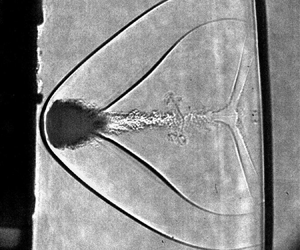
In figure 7, the projectile is coming from the left and the projectile bow shock is seen to process the drop. Then, the shock structure develops around the drop. In contrast to a solid sphere, there is no separation shock at the drop equator due to the change in the boundary condition. The wake shock does appear and its two termini are the base of the turbulent multiphase wake, and the bow shock; this bell shape of the wake shock is consistent among all cases.
For both the experiments and simulations, time is zero when the bow shock first intercepts the drop. In figures 9 and 10, the experimental snapshots for drops 3 and 6B are compared with the simulations, respectively. The angle of the main shock is steeper in the free stream for drop 3 in comparison with drop 6B due to the larger Mach number.
Comparison of shadowgraphs (above) vs numerical schlieren (below) for drop 3. Length scale represents the initial drop diameter.

Comparison of shadowgraphs (above) vs numerical schlieren (below) for drop 6B. Length scale represents the initial drop diameter.

The simulation results are in good agreement with the experiments and properly capture the position and shape of the main shock in front of the drop. The recompression shock is significantly harder to model as it is affected by some of the wake dynamics behind the drop. Overall, good agreement in shock position and shape has been obtained, providing confidence in the simulation results, and the dominant features can be captured in the simulations.
The initial transient in the shock dynamics around the drop is similar to what is observed for a rigid sphere, except for some behaviour in the wake region. Numerical schlieren images with highlighted flow features are provided in figure 11. The simulation results are qualitatively similar to what has been observed for the shock–cylinder interaction problems in the literature (Bryson & Gross Reference Bryson and Gross1961). First, the shock intercepts the front face of the drop and is reflected; this shock forms the bow shock over the drop. Following the terminology in Bryson & Gross (Reference Bryson and Gross1961), a curved ‘Mach shock’ and contact discontinuity form, establishing a triple point on the incident shock. Note this triple point is three-dimensional and revolves around the centre axis. Again, similar to Bryson & Gross (Reference Bryson and Gross1961), a second ‘Mach shock’ and contact discontinuity form, coming to a triple point on the initial ‘Mach shock’.
Simulation results at drop 6B conditions. Comparison of the initial transient for shock–drop (top) and shock–sphere interactions (bottom). Ref. S = reflected shock, Rec. S. = recompression shock, S.S. = separation shock, C.D. 1 = contact discontinuity, M.S. = Mach shock, T.P. = triple point, V.P. = vortical protuberance. Terminology from Bryson & Gross (Reference Bryson and Gross1961).

The separation shock does not appear on the drop; this is because of the partial-slip boundary condition on the drop surface. There is an additional feature that is not observed in shock–cylinder interactions: a protuberance that arises on the back of the drop and initially has a smaller radius. This feature comprises vortical structures, which rotate in the opposite direction to the upcoming first Mach shock that generates them after colliding in the wake region.
7. Drop displacement and flattening, and comparison with existing models
Several researchers have characterized the displacement and flattening of drops in high-speed flow (Engel Reference Engel1955, Reference Engel1958; Reinecke & McKay Reference Reinecke and McKay1969; Hébert et al. Reference Hébert, Rullier, Chevalier, Bertron, Lescoute, Virot and El-Rabii2020; Wang et al. Reference Wang, Hopfes, Giglmaier and Adams2020). Drop deformation is primarily driven by the difference in pressure between the gas at the stagnation point on the windward face of the drop and the decreasing pressure of the gas as it traverses the drop surface to the equator (Engel Reference Engel1958). In this section, a comparison between experimental observations and computations is made for drop diameter and flattening; these data are compared with existing predictive models in the literature. Moreover, the computations are analysed to investigate the drop deformation mechanics using cut planes showing pressure and velocity contours.
As in Hébert et al. (Reference Hébert, Rullier, Chevalier, Bertron, Lescoute, Virot and El-Rabii2020), the displacement of the mist leading edge (MLE) from its initial position was used as a proxy for the displacement of the drop centre of mass, which cannot be seen in shadowgraphs. The complete data set and the process by which the location of the MLE was determined are discussed in Appendix C. Those data indicate an average experimental value and standard deviation for a drag coefficient of  $C_D=2.32\pm 0.76$. This is nominally consistent with Hébert et al. (Reference Hébert, Rullier, Chevalier, Bertron, Lescoute, Virot and El-Rabii2020) (
 $C_D=2.15$) and Pilch et al. (Reference Pilch, Erdman and Reynolds1981) (
 $C_D=2.52$), bringing confidence to the current results. A subset of experimental and computational displacement data for drops 3, 4 and 6B are presented, along with error bars, in figure 12(a). Drops 3 and 4 were chosen because those data were taken at nominally the same Mach 5 condition, so repeatability could be assessed. Drop 6B was a Mach 3 shot, which represents the largest available contrast in Mach/Weber number in this dataset (see table 3). The computational predictions fall within the error bars for drop MLE displacement.
(a) Non-dimensional displacement of MLE and (b) non-dimensional diameter for drops 3, 4 and 6B, comparing simulation output with experimental data.

Experimental and computational drop flattening data for drops 3, 4 and 6B are compared in figure 12(b) with three flattening models found in the literature. The Reinecke & Waldman (Reference Reinecke and Waldman1975) model is a piecewise function where drop diameter is a function of the maximum pressure coefficient on the drop. The TAB model from O'Rourke & Amsden (Reference O'Rourke and Amsden1987) approximates the water drop as a constant-mass spring–damper system, where the restoring force is provided by drop surface tension while the drop viscosity dissipates energy. Inputs to this model are the Weber and Ohnesorge numbers, along with a constant that we have set as  $C_2=2$, which is nearly the same value for the constant as in Daniel et al. (Reference Daniel, Guildenbecher, Delgado, White, Reardon, Stauffacher III and Beresh2023). The nonlinear TAB (NTAB) model from Schmehl (Reference Schmehl2002) introduces additional terms to account for the deformation of the liquid drop toward an ellipsoidal shape. Inputs to this model are the Weber and Reynolds numbers, and a constant which, as in the TAB model, we have set as
 $C_2 = 2$. Both the TAB and NTAB models include
 $1/We_{A2}$ or
 $1/Re_{A2}$ terms, which decrease to very small values in this study; consequently, the growth rates predicted by each model for drops 3, 4 and 6B are almost indistinguishable when plotted, and only the model results for drop 6B are plotted in figure 12(b). Drops 3 and 4 exhibit similar flattening trends, but differ from one another enough that their error bars barely overlap. This indicates that there is a statistical spread in the flattening data. The root-mean-square difference between the models and experiment is approximately 5 %–10 %. A so-called ‘burst’ is highlighted in figure 12(b) as the drop diameter temporarily changed substantially when a chunk of the drop was cleaved off and entrained into the wake.
In contrast to the Reineke correlation, and the TAB/NTAB deformation models, Su et al. (Reference Su, Patterson, Reitz and Farrell1996) present a drop-breakup model, the basis of which is derived from KH and RT linear-stability analysis. This KH–RT hybrid model was designed to analyse the breakup of liquid sprays at velocities of  ${\approx }100\ {\rm m}\ {\rm s}^{-1}$ in a near-standard-temperature-and-pressure environment with
 $We_A<1000$. The times calculated for liquid drop breakup for cases 1–6B by this hybrid model are
 ${\approx }1\ \mathrm {\mu }$s for the RT mode and
 ${\approx }500\ \mathrm {\mu }$s for the KH mode. These calculated breakup times differ greatly from the observed drop-breakup times in this work and from the Rayleigh breakup time
 $t_{C2}$ computed in prior high-speed aerobreakup research. It is determined that the hybrid KH–RT model presented by Su et al. (Reference Su, Patterson, Reitz and Farrell1996) is not applicable to these flow conditions. This motivates further discussion of the linear- and nonlinear-instability regimes, as is done in § 8.
8. Instability mechanisms and models
Linear- and nonlinear-stability analyses are used to attempt to explain the developing structure at the liquid–air interface with the ultimate aim of eventually predicting drop demise. Computational results at early breakup times motivate a linear-stability analysis. A disconnect between the structures observed in both the computations and experiments and those predicted by the linear-stability analysis motivates a nonlinear-stability analysis. A comparison of the present work with that in the literature is made.
8.1. Computational results for early breakup time
The simulated drop exhibits ripples across its surface right after its interaction with the projectile bow shock (figure 13). The drop starts forming distinct annular structures and those structures keep growing throughout the test time. The shape of the back of the drop takes the characteristic ‘cupcake’ shape seen in lower-Mach-number experiments and simulations (Meng & Colonius Reference Meng and Colonius2018), but the front face is different, as it is not smooth, which is the result of higher shear in the present experiments.
Three-dimensional water volume fraction contours of 0.1 for drops 3 and 6B at early stages.

8.2. Simple linear-stability model for early breakup time
A simple treatment of the stability problem at the drop/gas interface is presented in this section to estimate the importance of shear, acceleration, viscosity, surface tension and geometry (aspect ratio) for early breakup times. The drop is sketched in figure 14(a). It is assumed that the front face takes the form of an ellipse as it deforms. Figure 14(b) shows a schematic of the classical stability treatment of an accelerated interface from Funada & Joseph (Reference Funada and Joseph2001) of the Kelvin (Reference Kelvin1871) and Helmholtz (Reference Helmholtz1868) instability. Here, it is assumed that the initial stability problem can be treated as a locally accelerated interface,  $\zeta (x',t) = \zeta _0 \exp ( {\rm i} \kappa x' + s t )$, and the stability analysis is locally valid as a function of
 $\phi$ from the stagnation point of the drop. Funada & Joseph (Reference Funada and Joseph2001) show, just after their (2.18), that the growth rate is
 \begin{align} s &={-} {\rm i} \kappa \frac{\rho_g u_g + \rho_d u_d} { \rho_g + \rho_d } \underbrace{- \frac{\kappa^2 (\mu_g + \mu_d)}{\rho_g + \rho_d } }_{Viscosity} \pm\left[ \underbrace{\frac{\kappa^2 \rho_g \rho_d \left(u_g - u_d \right)^2 }{(\rho_g + \rho_d)^2}}_{Shear} \underbrace{- \frac{\kappa a_{{\perp}} (\rho_g - \rho_d)}{\rho_g + \rho_d}}_{Acceleration} \right. \nonumber\\ & \quad \left. \underbrace{- \frac{\kappa^3 \sigma}{\rho_g + \rho_d} }_{{Surface\ tension}} \underbrace{+ \frac{\kappa^4 (\mu_g + \mu_d)^2}{(\rho_g + \rho_d)^2} + 2{\rm i} \kappa^3 \frac{(\rho_g \mu_d - \rho_d \mu_g) (u_g-u_d)}{(\rho_g + \rho_d)^2} }_{Viscosity} \right]^{1/2}. \end{align}
Here, four combinations of terms in (8.1) that might drive/damp instability growth are labelled as shear, acceleration, viscosity and surface tension. These terms are estimated as a function of  $\phi$ along the front face of the drop for various flow conditions and drop geometries. This was done by considering the real parts of the growth rate,
 ${\rm Re} (s)$, for each term while setting the others to zero.
(a) Schematic of deformed drop, exaggerated for sketch. (b) Adaptation of treatment by Drazin & Reid (Reference Drazin and Reid2004) and Funada & Joseph (Reference Funada and Joseph2001).

First,  $a_\perp = a_\perp (\phi )$ must be found, which is the acceleration normal to the interface to which a non-inertial reference frame (
 $x'-z'$) is fixed. The acceleration is assumed to be constant, which is supported by our data in figure 12 and data in Hébert et al. (Reference Hébert, Rullier, Chevalier, Bertron, Lescoute, Virot and El-Rabii2020). The acceleration parallel to the interface,
 $a_\parallel$, is assumed to negligibly affect the stability problem given that
 $\zeta$ is small and in the regime treated by small disturbances. That is, the component pertinent to the stability problem is only
 $a_\perp$. The front face of the drop is estimated to take the form of an ellipse as
 $F(x,y,z) = 0 = (z/c)^2 + (y/b)^2 - 1$. Then, the unit normal,
 $\underline {\hat {n}} = \boldsymbol {\nabla } F / |\boldsymbol {\nabla } F|$, can be used to calculate the needed quantities to approximate the acceleration as a function of
 $\phi$,
 $\tan (\phi _n) = (c/b)^2 \tan (\phi )$ and
 $a_\perp = |\underline {a}| \cos (\phi _n)$. The magnitude of acceleration is the drag force divided by the drop mass:
 \begin{equation} |\underline{a}| = \frac{F_d}{m_d} = \frac{3 \rho_2 C_d U_{2LF}^2}{4 \rho_d d} = \frac{3 C_d q_2}{2 \rho_d d}, \end{equation}
where  $q_2=1/2 \rho_{2} U_{2LF}^2$ is the dynamic pressure based on state 2 in the laboratory frame, and
 $C_d$ is the drag coefficient of the drop which is estimated to be a constant
 $C_d\approx 2.32$ (figure 12).
Next,  $u_g(\phi )$ and
 $\rho _g(\phi )$ must be found. A modified version of Newton's inclination method is used to find the pressure coefficient as
 \begin{equation} C_p(\phi) = \frac{p_g(\phi)-p_2}{\dfrac{1}{2} \rho_2 U_{2LF}^2} = \frac{p(\phi)-p_2}{q_2} = C_{p\,{max}}\cos^2(\phi_n).\end{equation}
Here, it is noted that the modified form of Newton's inclination method was taken from Lees (Reference Lees1956), who used data for the front face of a hemispherical cylinder from Stine & Wanlass (Reference Stine and Wanlass1954) to support the simple model at Mach and Reynolds numbers relevant to this work. The maximum pressure coefficient is calculated from the stagnation pressure at the drop face calculated in § 3 as  $C_{p\,{max}} = (p_{sd} - p_2)/q_2$. Then, the Mach number, density and temperature of the gas at the interface may be calculated as a function of
 $\phi$ as
 \begin{equation} \frac{p_{sd}}{p_g(\phi)} = \left(\frac{T_{sd}}{T_g(\phi)} \right)^{{\gamma}/({\gamma-1})}= \left(\frac{\rho_{sd}}{\rho_g(\phi)} \right)^{\gamma} = \left (1 + \frac{\gamma-1}{2} M_g(\phi)^2 \right)^{{\gamma}/({\gamma-1})},\end{equation}
which yields the velocity,  $u_g(\phi ) = M_g(\phi ) \sqrt {\gamma p_g(\phi )/\rho _g(\phi )}$.
The terms of (8.1) can now be estimated for an example condition, drop 3. This is done to understand which of shear, acceleration, viscosity and surface-tension terms are relevant on the drop face. In figure 15(a,c,e), the flow parameters along the front face of the drop are shown as a function of  $\phi$. The solid lines are from Newton's inclination method, calculated by (8.3) and (8.4) and the dots are CHAMPS-CFD (Cartesian higher-order adaptive multiphysics solver; computational fluid dynamics) data for inviscid flow past a rigid sphere. Agreement between the inclination method and the CFD data is sufficient to justify using the former to estimate the four relevant terms in the growth rate ((8.1)). The shear (green), acceleration (red), viscosity (magenta) and surface-tension (blue) terms are shown as semitransparent surfaces in figure 15(b,d,f). Here, the negative of the surface-tension term is plotted so it may be presented in log space (the surface-tension term will always be negative and serve to dampen the instability). Also inset in black is the drop profile and aspect ratio (
 $b/c$). Also, the growth rate is normalized by the time scale
 $t_{C2}$ from (1.5).
Estimated flow parameters (a,c,e) and growth rate (b,d,f) for drop aspect ratios,  $b/c=(1,2,4)$, respectively, for drop 3. The progression of
 $ab/cd/ef$ shows the effects of a drop becoming more elliptical (deforming). The lines and dots in (a,c,e) are the result of Newton's inclination method and inviscid CFD simulations for a solid sphere, respectively. The different surfaces in (b,d,f) correspond to the shear, acceleration, viscosity and surface-tension terms in (8.1). Inset in (a,c,e) is a trace of the drop shape in black.

Upon inspecting figure 15, it is apparent that viscosity and surface tension are not relevant in this simplified analysis, particularly at larger disturbance wavelength. More interestingly, as the aspect ratio,  $b/c$, is increased, the terms that dominate the growth in (8.1) change. For a spherical drop, the shear term appears to dominate everywhere except near the stagnation point, where the acceleration term is most prominent. As the drop aspect ratio is increased from
 $b/c=1$ to
 $b/c=2$ and then an exaggerated
 $b/c=4$, the acceleration term appears to become more dominant. This is because the profile of the front face of the drop is becoming flatter; that is, the acceleration and surface-tension terms nominally stay the same but the shear term is largely reduced because
 $u_g(\phi )$ is smaller. This is the primary takeaway from this simplified analysis. This effect would be further exaggerated if
 $u_d(\phi )$ were permitted to vary from zero. The effect of
 $u_d(\phi )$ being non-zero is not dominant, as estimates of growth rate assuming
 $u_d(\phi ) \approx F u_g(\phi )$ with
 $F=0.25,0.5$ were performed and the results in figure 15 are not changed substantively; that is, increasing the drop aspect ratio is far more effective in reducing
 $u_g(\phi )$.
An additional takeaway from figure 15 is the broadband and complex nature of the most-amplified instability at early times. A range of wavelengths are amplified and the spectrum changes as the drop deforms. This analysis is a clear example of the need for high-quality images of the front face of the drop similar to those in Theofanous (Reference Theofanous2011). This simple analysis may also explain why the drop face in that work is smooth.
Treating the stability problem as a linearly perturbed interface that grows exponentially presents inconsistencies with experimental results for late breakup times. For the conditions encountered in this experimental campaign, the linear growth rate is given by (8.1) and is maximized for wavelengths ( $\lambda \approx 30\ \mathrm {\mu }$m) smaller than those observed in shadowgraph images; that is, the resolution of those images (
 ${\approx }21.5\ {\rm pixels}\ {\rm mm}^{-1} \approx 46.5\ \mathrm {\mu }{\rm m}\ {\rm pixel}^{-1}$), was not high enough to discern such small waves from image noise. Evaluating (8.1) at the stagnation point for drop 4 yields the linear amplification curve in figure 16(a). A shadowgraph image showing the incipient surface sawtooth profile of drop 4 is presented in figure 16(b). The growth rate
 $s$ is maximized for a surface instability of
 $\lambda \approx 30\ \mathrm {\mu }$m, yet the wavelength of the incipient sawtooth profile is
 ${\approx }0.5\unicode{x2013}1.0$ mm. This observation indicates a shortcoming in the linear-stability treatment and is consistent with observations in Reinecke & McKay (Reference Reinecke and McKay1969), Pilch & Erdman (Reference Pilch and Erdman1987), Joseph et al. (Reference Joseph, Belanger and Beavers1999) and Theofanous (Reference Theofanous2011), among others.
(a) Linear growth rate ( $s$) vs wavelength (
 $\lambda$) per (8.1) for drop 4 at the stagnation point showing maximum exponential growth rate at
 $\lambda \approx 30\ \mathrm {\mu }$m. (b) Incipient sawtooth profile of drop 4; average wavelength between ripple peaks
 ${\approx }\,990\ \mathrm {\mu }$m.

8.3. Experimental and computational results for late breakup time and comparison with the literature
The spatial resolution of the simulations is sufficient to capture concentric rings on the drop windward face, which the authors believe to be physical (figure 17). The exact structure, number of rings and bursts may depend on the mesh and numerical noise seeding initial instabilities; this is because of the Cartesian mesh imprint. However, a simulation sensitivity analysis was performed by increasing spatial resolution and that effort showed the main flow features are not substantively changed with increasing resolution.
Schematic showing the evolution of ‘bursts’ and front face instabilities for drop 3 for late breakup times.

In figure 18, numerical and experimental shadowgraphs are compared for drop 6B at later non-dimensional times. The computations are performed with no surface tension. Given the apparent qualitative agreement between experiment and computation, this brings confidence to the assumption made in the computations, at least for macroscopic characterization. The boundary layer cannot be resolved as a consequence of resolution constraints, as well as any microscopic drop generation due to smaller-scale instabilities. The serrated or ‘sawtooth’ front face seen at  $\tau =1.17$, and already reported in the literature (Reinecke & McKay Reference Reinecke and McKay1969) is present in both the experiments and simulations.
Comparison of experimental shadowgraphs (above) vs numerical shadowgraphs (below) for drop 6B at three different times.

In figure 19, the results from the present study and Hébert et al. (Reference Hébert, Rullier, Chevalier, Bertron, Lescoute, Virot and El-Rabii2020) are compared at similar conditions and times. The shock and wake structures appear to be similar, bringing confidence to the current results. More interestingly, the front surface of the drop appears to show a large-scale incipient ‘sawtooth’ or ‘fingering’ profile. Figure 20 shows results from Reinecke & McKay (Reference Reinecke and McKay1969) (top left), Hébert et al. (Reference Hébert, Rullier, Chevalier, Bertron, Lescoute, Virot and El-Rabii2020) (top right) and results from the present work (bottom). The results from the present work are for different  $\tau$ but relatively similar
 $We_{A2}$. The non-dimensional time could potentially be explained by differing initial conditions in the three experiments. The different methods of suspending the drop could induce different initial conditions to the stability problem. However, the flow topology seems similar near the end of the breakup process. These fingering structures are similar to what is seen on the front face of the computations at later times (figure 17). Moreover, Pilch et al. (Reference Pilch, Erdman and Reynolds1981) and Pilch & Erdman (Reference Pilch and Erdman1987) suggest something similar in their figure 1 for ‘catastrophic breakup’. From Pilch & Erdman (Reference Pilch and Erdman1987), ‘[l]arge-amplitude, long-wavelength waves ultimately penetrate the drop creating several large fragments before wave crest stripping can significantly reduce the drop mass’. This implies a race between SIE and the larger, long-wavelength waves that penetrate the drop suggested by Joseph et al. (Reference Joseph, Belanger and Beavers1999) among many others. That is, we are implying that the results from Joseph et al. (Reference Joseph, Belanger and Beavers1999) and Theofanous & Li (Reference Theofanous and Li2008) are not in conflict, as is sometimes understood, but the results are complementary. The simple linear-stability analysis done in § 8.2, and the analysis done in Joseph et al. (Reference Joseph, Belanger and Beavers1999) is probably not appropriate for long non-dimensional times when these ‘fingering’ structures appear. It is most likely that a nonlinear analysis would be required. Not imaging the front face of the drop at late breakup times is a shortcoming of the experimental design and must be remedied in future work.
Comparison of Hébert et al. (Reference Hébert, Rullier, Chevalier, Bertron, Lescoute, Virot and El-Rabii2020) drops (above) with drops 5B and 3, noting they are recorded at similar non-dimensional (and dimensional) times and similar non-dimensional (and dimensional) conditions.

Comparison of Reinecke & McKay (Reference Reinecke and McKay1969) drop (upper left) with drop 6B (lower left), showing similar sawtooth profile on windward side. The Hébert et al. (Reference Hébert, Rullier, Chevalier, Bertron, Lescoute, Virot and El-Rabii2020) drop (upper right) shows incipient sawtooth formation, also visible on drop 4 (lower right); given more time, both of these drops would (most likely) develop a more pronounced sawtooth profile.

8.4. Proposed explanation of large-scale structures at late breakup times
Taking the maximum growth rate from figure 16, and assuming an initial amplitude of  $\zeta _{0}=1\ \mathrm {\mu }$m, the instability is expected to grow to a size comparable to that of the drop itself in just a few microseconds; yet, no drop studied in this experimental campaign breaks up that quickly. As such, and consistent with the approach in Pilch et al. (Reference Pilch, Erdman and Reynolds1981) and Pilch & Erdman (Reference Pilch and Erdman1987), a ‘large-amplitude’ treatment of the stability problem is proposed to account for the fundamental discrepancy in the size of the observed structure at late breakup times.
Pilch et al. (Reference Pilch, Erdman and Reynolds1981), citing Davies & Taylor (Reference Davies and Taylor1950), Garabedian (Reference Garabedian1957) and Fishburn (Reference Fishburn1974), used a model where the growth rate became a function of drop acceleration and instability wavelength after a certain instability size threshold was reached. According to this model, the growth of a surface instability on the windward face of a drop is equivalent to the penetration of liquid by an open bubble of gas, which is a common assumption in the treatment of nonlinear RT instability (Kull Reference Kull1991; Zhou et al. Reference Zhou2021). The growth rate is constant in time and is written as
 \begin{equation} \frac{{\rm d}\zeta}{{\rm d} t}_{nonlin} = F\sqrt{(1-\epsilon )a\lambda},\end{equation}
where  $a$ is the drop acceleration,
 $\epsilon$ is the density ratio
 $\rho _{g}/\rho _{d}$ and
 $\lambda$ is the wavelength of a surface instability. Here,
 $F$ is given by
 \begin{equation} F = Fr\sqrt{\left(1-4 \frac{{\rm \pi}^{2} \sigma}{(1-\epsilon)\rho_{d}a\lambda^{2}}\right)},\end{equation}
which reduces to the Froude number ( $Fr$) in the case of zero surface tension. The Froude number was numerically calculated by, among others, Birkhoff (Reference Birkhoff1955), Garabedian (Reference Garabedian1957) and Kull (Reference Kull1986) to be
 $\approx 0.23$ for a two-dimensional planar bubble and
 $\approx 0.36$ for a three-dimensional bubble. Equation (8.5) gives an upper bound for the velocity with which an open bubble penetrates a volume of liquid. Because this velocity constitutes an upper bound for the gas penetration velocity into a volume of liquid, Pilch et al. (Reference Pilch, Erdman and Reynolds1981) defines a transition time,
 $t_{t}$, between the linear (exponential) growth and the nonlinear (constant rate) growth as the time when the growth rates are equal:
 \begin{equation} \left. \frac{{\rm d}\zeta}{{\rm d} t}_{lin} \right|_{t_t} = \zeta_0 s \exp( {\rm i} \kappa x' + s t_t ) = \left. \frac{{\rm d} \zeta}{{\rm d} t}_{nonlin} \right|_{t_t} = F\sqrt{(1-\epsilon )a\lambda}.\end{equation}
Considering only the real parts of the growth rate, ignoring the effects of viscosity and restricting the analysis to the windward face of the drop, where  $u_{g} \approx 0$, this relation can be solved for the transition time as
 \begin{equation} t_{t} = \frac{\ln\left( {\dfrac{F\sqrt{(1-\epsilon)a\lambda}}{s \zeta_{0}}} \right) }{s}.\end{equation}
The transition time between the linear- and nonlinear-instability growth regimes is a function of drop acceleration,  $a$, surface instability wavelength,
 $\lambda$, the initial disturbance magnitude,
 $\zeta _{0}$, and the exponential instability growth rate,
 $s$. Pilch et al. (Reference Pilch, Erdman and Reynolds1981) states that there must exist a smooth transition between the exponential and constant-rate instability growth regimes. For simplicity, the surface instability growth is instead here modelled as a piecewise function. For the conditions of drop 4, the transition time
 $t_{t}$ was evaluated for a range of different initial disturbance magnitudes and disturbance wavelengths. Figure 21(a) shows that, for plausible initial disturbance magnitudes of the order of 1
 $\mathrm {\mu }$m and surface instability wavelengths of the order of those seen in shadowgraph images, surface instability growth transitions to the nonlinear regime well before
 $\tau = 1$ is reached. That is, for much of the drop-breakup process, surface instability growth is nonlinear and can be modelled as in (8.5) rather than the exponential model that applies for small instability magnitudes.
(a) Non-dimensionalized transition time  $\tau _{t} = t_{t}/t_{c2}$ for drop 4 for a range of initial disturbance magnitudes
 $\zeta _{0}$ and instability wavelengths
 $\lambda$. (b) Penetration rates for drop 4 calculated for different
 $\lambda$ and
 $\zeta _{0}$. (c) Surface instability amplitudes as a function of time for drop 4 computed for different
 $\lambda$ and
 $\zeta _0$ according to (8.9).

The instability amplitude  $\zeta _{f}$ at any given time
 $t$ can be computed by adding the integrals of instability growth rate over time in both regimes as
 \begin{equation} \zeta_{f} = \int_{0}^{t_{t}} \zeta_{0}s\,{\rm e}^{st} \,{\rm d} t + \int_{t_{t}}^{t_{f}} F\sqrt{(1-\epsilon )a\lambda} \,{\rm d} t = \zeta_{0}\,{\rm e}^{s t_{t}} + (t_{f}-t_{t}) F\sqrt{(1-\epsilon )a\lambda}.\end{equation}
It is assumed that there is a  $\zeta _{0,M}$ which is the initial disturbance necessary to maximize instability growth at the instability wavelength observed in shadowgraph photos or a numerical simulation,
 $\lambda _{ob}$. This is found by
 \begin{equation} \left. \frac{\partial\zeta_{f}}{\partial\lambda}\right|_{\lambda_{ob},\zeta_{0,M}} = 0. \end{equation}
Assuming surface tension is negligible, a simplified relation for  $\zeta _{0,M}$ using (8.10) is
 \begin{equation} \zeta_{0,M} = \frac{Fr\sqrt{a(1-\epsilon)\lambda_{ob}}}{\exp{\dfrac{1}{2}(t_{f}\sqrt{2{\rm \pi} a (1-\epsilon)/(\lambda_{ob}(1+\epsilon))}+\ln({2{\rm \pi} a (1-\epsilon)/(\lambda_{ob}(1+\epsilon))}))}}.\end{equation}
Now, the developed model may be evaluated. For example, figure 16 shows drop 4 at time  $t_{f} = 14.4\ \mathrm {\mu }$s, with
 $\lambda _{ob} = 990\ \mathrm {\mu }$m. The values
 $a$ and
 $\epsilon$ for this drop were computed to be
 $1.1\times 10^7\ {\rm m}\ {\rm s}^{-2}$ and 0.025, respectively. Here,
 $Fr = 0.23$ is assumed for an annular bubble (a planar bubble revolved around the drop axis). From (8.11),
 $\zeta _{0,M}=14.4\ \mathrm {\mu }$m for drop 4. Table 4 summarizes these results for drop 4, with those for drop 6B, based on the surface instability wavelength measured in shadowgraph images and simulations. For both drops, the transition time
 $t_{t}$ is well below the time of drop impact, indicating that, according to this model, much of the drop's evolution is governed by nonlinear growth.
Observed wavelength  $\lambda _{ob}$, transition time
 $t_t$, initial disturbance
 $\zeta _{0,M}$, nonlinear growth rate predicted by (8.5) for experimental and simulation data. Observed growth rate for simulations from linear fits in figure 22, noting growth rate not directly observed in experiments.

In figure 21(b), the blue curve shows the growth rate according to this model for drop 4 given  $\lambda _{ob} = 990\ \mathrm {\mu }$m from the shadowgraphs and with a predicted initial disturbance amplitude of
 $\zeta _{0,M}=14.4\ \mathrm {\mu }$m. The red curve uses the same model but the input wavelength is not that observed from the shadowgraphs, but the wavelength that maximizes the linear growth rate in figure 16(a), which is
 $\lambda _{lin} = 28\ \mathrm {\mu }$m; here, the initial disturbance amplitude is predicted to be
 $\zeta _{0,M}=0.25$ nm. Finally, the green curve represents the result of assuming
 $\lambda _{lin} = 28\ \mathrm {\mu }$m with the initial disturbance amplitude estimated to be
 $\zeta _{0,M}=14.4\ \mathrm {\mu }$m from the prior case. Note the smaller effective growth rate and transition time for cases with
 $\lambda _{lin} = 28\ \mathrm {\mu }$m compared with the case with
 $\lambda _{ob} = 990\ \mathrm {\mu }$m. This model predicts that small-wavelength disturbances transition to the nonlinear regime relatively quickly, effectively capping the growth rate of those disturbances that would otherwise dominate. To highlight this effect, the time integral of the data in figure 21(b) yields the calculated instability magnitude, which is shown in figure 21(c).
The plausibility of the calculated initial disturbance amplitudes can be assessed. An upper bound for initial disturbance amplitude may be estimated from the experiments by inspecting the pre-shot shadowgraphs, as those data appear smooth. Given camera resolution, the initial disturbances may be no larger than 50  $\mathrm {\mu }$m. A lower bound could be estimated by considering the conditions for which the flow local to a disturbance violates the continuum assumption. That length scale is estimated to be
 $\approx$1–10 nm by considering the local Knudsen number to be of order unity. These upper and lower bounds bracket our predicted initial disturbance amplitudes.
The simulations can be used to assess the efficacy of this model, even if the experimental design precludes direct comparison of the growth rate. To track the mean location of the drop surface, an ellipse was fitted to the windward face as assumed to be marked by the position of the 0.01 volume fraction ( $\alpha _l = 0.01$) isosurface. These data were used to compute the acceleration for each case. The amplitude of a disturbance was found by tracking the difference between adjacent ripple peaks and troughs. The adjacent peak/trough pairs were tracked backward in time via a Gaussian peakfinder (O'Haver Reference O'Haver1997). The initial guess for each peak location is given by the prior timestep, as is done in tagging velocimetry (Segall et al. Reference Segall, Shekhtman, Hameed, Chen and Parziale2023). Figure 26 in Appendix D shows a snapshot of peak/trough fitting for drop 6B. Figure 22 shows the computed disturbance amplitude as a function of time for the simulations of drops 4 and 6B (the simulation of drop 3 is used for drop 4 because the flow conditions are nearly identical between the two drops). The computational data indicate a clear transition between growth regimes. The agreement between the model and the simulations during the linear stage is difficult to assess given the model assumptions and spatial resolution in the computations; the same is true of the existence and timing of transition between regimes. Finally, the model/computational agreement for the nonlinear-instability growth rate is good in each case. The value of
 $Fr \sqrt {\lambda a}$ ((8.5)) computed in each case matches the computations to within 25 % (for case 6B) and to within 5 % (for case 4); this was determined by comparing computed nonlinear growth rate with the slopes of the linear fits in figure 22.
Non-dimensionalized instability amplitude  $\zeta /d_{d}$ vs non-dimensional time
 $t/t_{c2}$ for simulated (a) drop 4 and (b) drop 6B.

The qualitative agreement between the simple nonlinear model from Pilch et al. (Reference Pilch, Erdman and Reynolds1981) and the simulations brings confidence to the approach. Furthermore, the assertion that much of the aerobreakup process observed in these experiments is likely in the nonlinear regime is strengthened. Finally, the authors believe this is a plausible hypothesis to explain why the wavelengths observed in experimental shadowgraphs are far larger than those predicted by linear-stability analysis.
9. Conclusion
Experiments and simulations of drop aerobreakup at high Mach and Weber numbers were carried out. High-speed backlit shadowgraph images of drops processed by bow shock waves at Mach numbers from 3.03 to 5.12 at sea-level ambient pressures were generated, and these images were compared with numerical simulations of drop aerobreakup. The high-speed images collected in this experimental campaign represent a potentially unique data set for these flow conditions.
A one-dimensional reacting gas dynamics model was applied to predict the conditions behind the bow shock wave of the projectile and the drop. That is, a double stagnation point flow problem was solved and it was found that the gas is nearly calorically perfect with a ratio of specific heats of  $\gamma =1.3$. This assumption was used to simplify the numerical simulations. Moreover, the aerobreakup Weber number,
 $We_A$, and Reynolds number,
 $Re_A$, increase along the stagnation streamline of the projectile by
 ${\approx }50\,\%$ and
 ${\approx }25\,\%$, respectively. Although these increases are appreciable, they most likely do not alter the drop-breakup regime, making this data set comparable to shock-tube aerobreakup studies. Additionally, accounting for the drop bow shock does change the Weber and Reynolds numbers, but, also most likely, not enough to change the breakup regime. The parameters
 $We_A$ and
 $Re_A$ are evaluated at state 2, behind the bow shock of the projectile, as a valid state of comparison for this work with the literature. Finally,
 $We_A = \rho _g U_{LF}^{2} d_{d} / \sigma$, so it essentially parameterizes the aerodynamic pressure on the drop; that is, the aerodynamic pressure increases
 ${\approx }50\,\%$ along the stagnation streamline of the projectile.
Experimental data for drop deformation and position were acquired and compared with simulations. Drop displacement data were used to approximate the drag coefficient for a liquid drop in aerobreakup. The approximate drag coefficient  $C_{d} = 2.32$ is consistent with the range of drag coefficients found in Pilch et al. (Reference Pilch, Erdman and Reynolds1981) and Hébert et al. (Reference Hébert, Rullier, Chevalier, Bertron, Lescoute, Virot and El-Rabii2020), among others. Drop displacement data were used to compute the acceleration to which the drops were subjected and drop deformation data were used to compute the degree of drop flattening before impact in support of drop surface instability analysis. Numerical simulations of drop aerobreakup reach similar values of
 $C_{d}$ and drop acceleration to those found in the experiments.
Observations of the shock structure and wake dynamics were made. Several differences between the shock structure around a deforming liquid drop and a rigid, solid sphere were identified. No separation shock at the drop equator is observed for deforming liquid drops. A vortical protuberance in the flow field is observed in the wake of liquid drops. A Mach-number dependence on the stability of the wake potentially explains the flow topology. Higher-Mach-number flows result in less chaotic wake structures with less apparent turbulent flow. Mass shedding from the drop equator is observed in simulations and shadowgraphs of liquid drops.
Linear-stability theory results from Funada & Joseph (Reference Funada and Joseph2001) were used to assess the dependence of growth rate on (a) location on the drop face, (b) instability wavelength, (c) relative contributions of shear, acceleration, surface tension and viscosity and (d) the shape of the drop. The calculations in this work determined that viscosity and surface tension likely do not play a significant role at these conditions. At the stagnation point, the acceleration term dominates the shear term, and this relation inverts as one moves from the stagnation point to the drop equator. Finally, drop shape has a significant role in determining which of the terms dominates the problem. That is, for flattened drops, the acceleration term's dominance tends to broaden and move towards the drop equator, minimizing the shear term's importance.
We identified a long-standing discrepancy in the literature where some researchers assert that linear-instability growth results in rapid and sudden drop breakup when instability amplitude becomes comparable to drop thickness (Reinecke & McKay Reference Reinecke and McKay1969; Joseph et al. Reference Joseph, Belanger and Beavers1999). Others assert that no such phenomenon is present and that drop breakup is governed exclusively by mass stripping (Theofanous & Li Reference Theofanous and Li2008; Theofanous Reference Theofanous2011). Surface instabilities predicted from Funada & Joseph (Reference Funada and Joseph2001) differ in amplitude and wavelength from those observed in either shadowgraph images or numerical simulations. Linear-stability analysis was insufficient for modelling late-stage aerobreakup because the predicted wavelengths were too small and the expected aerobreakup times were non-physically short. A model for nonlinear growth at large instability amplitudes was found in the literature (Pilch et al. Reference Pilch, Erdman and Reynolds1981) and further developed. This model treats the nonlinear (constant rate) surface instability growth as an analogue to bubble rise in a mass of liquid, which is common in nonlinear RT treatment (Kull Reference Kull1991; Zhou et al. Reference Zhou2021). The computed time of transition between the linear- and nonlinear-instability growth regimes was found to be less than  $\tau = 1$ for all drops studied, indicating that much of the aerobreakup process takes place in the nonlinear-instability growth regime. An analytical solution for the initial instability magnitude was derived; initial disturbances inferred from this analysis were found to be plausible for the experimental conditions (
 $\zeta _0\approx 1\unicode{x2013}10\ \mathrm {\mu }$m). This nonlinear-instability growth model may explain results for drop breakup in prior literature thought (or alleged) to be anomalous. That is, we are implying that the results from Reinecke & McKay (Reference Reinecke and McKay1969), Joseph et al. (Reference Joseph, Belanger and Beavers1999), Theofanous & Li (Reference Theofanous and Li2008) and Theofanous (Reference Theofanous2011) are not in conflict, as is sometimes understood, but the results are complementary.
Supplementary movies
Supplementary movies are available at https://doi.org/10.1017/jfm.2024.1092.
Acknowledgements
C.J. Croft and D. Wise of the Naval Surface Warfare Center Dahlgren Division in Dahlgren, VA were the test engineers who oversaw the rail-gun tests. Without their hard work and that of the entire rail-gun team, the tests would not be possible.
Thank you to Dr E. Marineau for his technical council and encouragement; efforts that go beyond the typical responsibilities of a program officer.
Thank you to P. McClelland and B. Fraser of the Stevens Institute of Technology machine shop for help with fabricating various parts of the experiment.
Thank you to Professors J. Shepherd and H. Hornung for their discussions on the stagnation point flow model that appears in § 3.
Thank you to Professor S. Lawrence of the University of Maryland for the generous loan of his Kirana high-speed camera.
Funding
A.R.D., J.D.L. and N.J.P. were supported by ONR-MURI grant N00014-20-1-2682. C.B. and M.V.-M. were supported by ONR grant N00014-22-1-2443. Dr E. Marineau of Code 351 is the Program Officer for both grants.
Declaration of interests
The authors report no conflict of interest.
Data availability statement
All data presented herein are ‘Distribution Statement A: Approved for public release, distribution is unlimited’. See JFM's research transparency policy for more information.
Appendix A. Stagnation point flow model details
The calculations to predict the flow along the stagnation streamline were performed with Cantera (Goodwin Reference Goodwin2003; Goodwin et al. Reference Goodwin, Moffat, Schoegl, Speth and Weber2022) using the SDT (Browne et al. Reference Browne, Ziegler, Bitter, Schmidt, Lawson and Shepherd2018) in MATLAB. The shock-jump conditions in the shock-fixed frame are used to calculate the change in conditions from the unprocessed gas upstream of the infinitely thin bow shock on the projectile, state 1, to that immediately downstream of the shock, state 2. The mass, momentum and energy conservation equations are
 $$\begin{gather} \rho_1 U_p = \rho_2 U_2, \end{gather}$$
 $$\begin{gather}P_1 + \rho_1 U_p^2 = P_2 + \rho_2 U_2^2 \end{gather}$$
and
 \begin{equation} h_1 + \tfrac{1}{2} U_p^2 = h_2 + \tfrac{1}{2} U_2^2.\end{equation}
The PostShock_fr function in the SDT solves (A1)–(A3) assuming thermodynamic equilibrium ( $T_{trans}=T_{rot}=T_{vib}$) but frozen chemical composition. For all conditions in table 1, estimates of vibrational relaxation time from White & Millikan (Reference White and Millikan1964) indicate that O
 $_2$ will have thermodynamically equilibrated but N
 $_2$ may be in vibrational non-equilibrium. However, even small levels of humidity appreciably reduce the relaxation time of N
 $_2$ (Bass & Raspet Reference Bass and Raspet1978; Bass, Ezell & Raspet Reference Bass, Ezell and Raspet1983). The relative humidity for each case was at least 30 %; as such, the thermodynamic equilibrium assumption is valid for both O
 $_2$ and N
 $_2$.
The flow along the streamline inside the shock layer is modelled as an inviscid, isentropic, one-dimensional compression where the mass flux linearly decreases from the state immediately behind the shock, state 2, to the state at the stagnation point on the projectile, state  $sp$, with no drop present. The linearly decreasing mass-flux assumption follows the work of Stulov (Reference Stulov1969) and Hong et al. (Reference Hong, Wang, Hu and Sun2020), noting that other researchers have also made similar assumptions and observations with regards to linearly varying mass flux, density or velocity (Hornung Reference Hornung1972; Olivier Reference Olivier1993, Reference Olivier2000; Wen & Hornung Reference Wen and Hornung1995; Leibowitz Reference Leibowitz2020; Yanes Reference Yanes2020). Browne et al. (Reference Browne, Ziegler, Bitter, Schmidt, Lawson and Shepherd2018) assumes that the linearly varying mass flux is
 \begin{equation} \rho U_{PF} = \rho_2 U_2 \left(1-\frac{x}{\varDelta_p} \right), \end{equation}
where the  $PF$ subscript refers to the projectile frame of reference. To solve the stagnation point problem, Kao et al. (Reference Kao, Ziegler, Bitter, Schmidt, Lawson and Shepherd2023) §§ 11.6 and 11.7 are followed. That work uses the temporal version of the thermicity formulation of the governing equations with a varying streamtube area. The conservation of mass equation is
 \begin{equation} A \rho U_{PF} = A_2 \rho_2 U_2.\end{equation}
Using (A4) and (A5), the product of the velocity,  $U_{PF}$, and the logarithmic area change parameter,
 $\alpha$, can be written as
 \begin{equation} U_{PF} \alpha = U_{PF} \frac{1}{A} \frac{{\rm d}A}{{\rm d}\kern0.7pt x} = U_{PF} \frac{1}{1-\varDelta_p} = \frac{\rho_2}{\rho} \frac{U_2}{\varDelta_p}.\end{equation}
Continuing to follow Browne et al. (Reference Browne, Ziegler, Bitter, Schmidt, Lawson and Shepherd2018), the governing equations are
 $$\begin{gather} \frac{{\rm d}\kern0.7pt x}{{\rm d} t} = U_{PF}, \end{gather}$$
 $$\begin{gather}\frac{{\rm d} P}{{\rm d} t} ={-}\rho U_{PF}^2 \left( \frac{\dot{\sigma} - U_{PF} \alpha }{\eta} \right), \end{gather}$$
 $$\begin{gather}\frac{{\rm d} \rho}{{\rm d} t} ={-}\rho \left( \frac{\dot{\sigma} - U_{PF} \alpha M^2}{\eta} \right), \end{gather}$$
 $$\begin{gather}\frac{{\rm d} U_{PF}}{{\rm d} t} = U_{PF} \left( \frac{\dot{\sigma} - U_{PF} \alpha}{\eta} \right) \end{gather}$$
and
 \begin{equation} \frac{{\rm d} Y_{k}}{{\rm d} t} = \frac{W_k \dot{\omega}_k}{\rho} \quad (k=1,2,\ldots K). \end{equation}
Here,  $\dot {\sigma }$ is the thermicity, which is written as
 \begin{equation} \dot{\sigma} = \sum_{k=1}^{K} \left[ \left(\frac{W}{W_k} - \frac{h_k}{c_p T} \right) \frac{W_k \dot{\omega}_k}{\rho} \right],\end{equation}
and  $\eta$ is the sonic parameter, which is written as
 \begin{equation} \eta = a_f^2(1-M^2).\end{equation}
The terms  $a_f$,
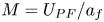 $M=U_{PF}/a_f$,
 $k$ and
 $K$ are the frozen sound speed, Mach number, species index and number of species, respectively. The terms
 $h_k$,
 $W_k$,
 $Y_k$,
 $X_k$ and
 $\dot {\omega _k}$ are the mass-specific enthalpy, molecular weight, mass fraction, mole fraction and net molar rate of production per unit volume, referring to species
 $k$, respectively. Finally, the terms
 $c_p$,
 $W$ and
 $x$ are the mass-specific heat at constant pressure, the mixture molecular weight and the distance from the shock, respectively. Equations (A7)–(A11) represent a series of 4+
 $K$ simultaneous ordinary differential equations. Integration begins at the shock (
 $x=t=0$) with initial conditions provided by the PostShock_fr function in the SDT which solves which (A1)–(A3).
The integration is made in time with the MATLAB solver ode15s, noting that position is solved with (A7). In this model, a fluid element along the stagnation streamline will approach the stagnation point with asymptotically vanishing velocity, so the choice of when to terminate the integration is arbitrary, and  $t_{end} = 50\varDelta _p/U_p$ is chosen in this work. In figure 23, the results of the stagnation point problem are presented for shot 3. The asymptotically vanishing velocity is evident, as the fluid element is no longer traversing an appreciable distance at 500
 $\mathrm {\mu }$s.
Time and velocity along the stagnation streamline for shot 3.

Appendix B. Governing equations for the detailed simulations
The governing equations for the detailed simulations are written as
 $$\begin{gather} \frac{\partial\alpha_{l}\rho_{l}}{\partial t} + \boldsymbol{\nabla}\boldsymbol{\cdot}( \alpha_{l}\rho_{l}\boldsymbol{u} ) = 0, \end{gather}$$
 $$\begin{gather}\frac{\partial\alpha_{g}\rho_{g}}{\partial t} + \boldsymbol{\nabla}\boldsymbol{\cdot}( \alpha_{g}\rho_{g}\boldsymbol{u}) =0, \end{gather}$$
 $$\begin{gather}\frac{\partial\rho\boldsymbol{u}}{\partial t} + \boldsymbol{\nabla}\boldsymbol{\cdot}( \rho\boldsymbol{u}\otimes\boldsymbol{u} + p \boldsymbol{\mathsf{I}} - \boldsymbol{\mathsf{T}} ) = 0, \end{gather}$$
 $$\begin{gather}\frac{\partial E}{\partial t} + \boldsymbol{\nabla}\boldsymbol{\cdot}[ ( E + p )\boldsymbol{u} - \boldsymbol{\mathsf{T}} \boldsymbol{\cdot} \boldsymbol{u} ] = 0, \end{gather}$$
 $$\begin{gather}\frac{\partial \alpha_{l}}{\partial t} + \boldsymbol{u}\boldsymbol{\cdot}\boldsymbol{\nabla}\alpha_{l} = 0. \end{gather}$$
Here, the two fluid phases are represented by the subscripts  $k = l,g$, referring to liquid and gas, respectively, and
 $\boldsymbol{\mathsf{T}}$ is the viscous stress tensor, which is given by
 \begin{equation} \boldsymbol{\mathsf{T}} = 2 \mu (\boldsymbol{\mathsf{D}} - \tfrac{1}{3} (\boldsymbol{\nabla} \boldsymbol{\cdot} \boldsymbol{u}) \boldsymbol{\mathsf{I}} ) , \end{equation}
where  $\mu$ is the molecular viscosity. The viscosity is calculated by following a simple mixture rule from Perigaud & Saurel (Reference Perigaud and Saurel2005) given by
 \begin{equation} \mu = \alpha_{l} \mu_{l} + \alpha_{g} \mu_{g}, \end{equation}
where  $\alpha _{k}$ is the volume fraction occupied and
 $\mu _k$ is the component viscosity. The velocity vector is given by
 $\boldsymbol {u}$,
 $p$ is the static pressure and
 $E = \rho ( e + \lvert \boldsymbol {u} \rvert ^{2}/2 )$ is the total energy. The internal energy and pressure are related by the stiffened gas equation of state,
 ${p_{k}} = (\gamma _{k}-1)\rho _{k}e_{k} - \gamma _{k}p_{k}^{\infty }$, with parameters
 $\gamma$ and
 $p^{\infty }$. Parameter
 $p^{\infty }$ allows liquid water to undergo metastable states at negative pressures. The total density and mass fraction, volume fraction and component density for each phase are related by
 \begin{equation} \rho Y_{k} = \alpha_{k} \rho_{k} , \end{equation}
where  $Y_{k}$ is the mass fraction,
 $\rho _{k}$ is the component density of either phase
 $k$ and
 $\rho$ is the total density. With this formulation, the volume fractions and mass fractions add up to one, i.e.
 $\alpha _{l} + \alpha _{g} = 1$ and
 $Y_{l} + Y_{g} = 1$. To numerically solve the governing multiphase (B1)–(B5), they are re-written in a slightly modified form which is given below in vector form
 \begin{equation} \frac{\partial\boldsymbol{W}}{\partial t} + \frac{\partial (\boldsymbol{F}^{x}_c+\boldsymbol{F}^{x}_d)}{\partial x}+\frac{\partial(\boldsymbol{F}^{y}_c+\boldsymbol{F}^{y}_d)}{\partial y} +\frac{\partial(\boldsymbol{F}^{z}_{c}+\boldsymbol{F}^{z}_{d})}{\partial z}+ \boldsymbol{\varSigma}= 0, \end{equation}
where the state vector,  $\boldsymbol {W}$, convective and viscous fluxes,
 $\boldsymbol {F}^i_c$ and
 $\boldsymbol {F}^i_d$, respectively, and an additional source term,
 $\varSigma (\boldsymbol {W},\boldsymbol {\nabla } \boldsymbol {W})$, are
 \begin{align} \boldsymbol{W} =
\begin{bmatrix} \alpha_{1}\rho_{1} \\ \alpha_{2}\rho_{2} \\
\rho u \\ \rho v\\ \rho w\\ E \\ \alpha_{1} \\
\end{bmatrix},\quad \boldsymbol{F}^i_c= \begin{bmatrix}
\alpha_{1}\rho_{1} u_{i}\\ \alpha_{2}\rho_{2} u_{i}\\ \rho
u_{x} u_{i} + p \delta_{xi} \\ \rho u_{y} u_{i} + p
\delta_{yi} \\ \rho u_{z} u_{i} + p \delta_{zi} \\ (E +p)
u_{i} \\ 0 \\ \end{bmatrix},\quad \boldsymbol{\varSigma} =
\begin{bmatrix} 0 \\ 0 \\ 0 \\ 0 \\ 0 \\ 0 \\ u
\boldsymbol{\nabla}\alpha_{1}\\
\end{bmatrix}\quad \text{and}\quad \boldsymbol{F}^i_{d} =
\begin{bmatrix} 0 \\ 0 \\ 0 \\ \tau_{ix}\\ \tau_{iy} \\
\tau_{iz} \\ \tau_{ij} u_{j}\\ 0 \\
\end{bmatrix}.
\end{align}
In (B10a–d),  $i$ and
 $j$ can be replaced by the Cartesian coordinate directions
 $x$,
 $y$ and
 $z$. In this formulation, the different components of
 $\boldsymbol {W}$ are treated as conserved variables except for the volume fraction advection equation which has been shown to improve the numerical robustness.
Appendix C. Complete drop displacement and flattening data and error analysis
Complete drop displacement and flattening data for all drops are included in figure 24. Experimental accelerations were determined by fitting a quadratic to this data. In figure 24(a), drop 2B appears to return to its initial location after some displacement; this is a measurement error that appears more pronounced because of the very small initial diameter of this drop. When the movement of this drop to higher values of  $\tau$ is plotted, the apparent reverse motion is much less significant.
(a) Non-dimensional displacement of MLE for all drops, with expected displacement curve assuming a constant drag coefficient of 2.32. (b) Non-dimensional diameter for all drops.

Error in the elapsed non-dimensional time since shock processing for each drop was calculated according to
 \begin{equation} (\delta \tau )^{2} = \left(\partial t \frac{\partial \tau}{\partial t}\right)^{2} + \left(\partial d_{d} \frac{\partial \tau}{\partial d_{d}}\right)^{2} + \left(\partial U_{A} \frac{\partial \tau}{\partial U_{A}}\right)^{2} + \left(\partial \rho_{g}\frac{\partial \tau}{\partial \rho_{g}}\right)^{2}.\end{equation}
The partial derivatives of  $\tau$ with respect to
 $t$,
 $d_{d}$,
 $u_{g}$ and
 $\rho _{g}$ are given, through taking derivatives of (1.5).
The measurement error of the drop diameter  $d_{d}$ was assumed to be
 $\pm$2 pixels, which was converted into a measurement error in metres by dividing 2 pixels by the camera resolution for that shot. The calculation error of gas density
 $\rho _{g}$ and local gas velocity
 $U_{A}$ were assumed to be 3 %. The error in measured time
 $t$ was assumed to be equal to the camera exposure time for that shot. Zero error was assumed for the density of liquid water.
Similarly, the error in non-dimensional drop displacement  $\Delta x$ was calculated according to
 \begin{equation} \left(\delta
\frac{\Delta x}{d_{d}}\right)^{2} = \begin{pmatrix}\delta
d_{d}\dfrac{\partial \dfrac{\Delta x}{d_{d}}}{\partial
d_{d}}\end{pmatrix}^{2} + \begin{pmatrix}\delta \Delta x \dfrac{\partial
\dfrac{\Delta x}{d_{d}}}{\partial \Delta x}\end{pmatrix}^{2}.\end{equation}
The error in drop displacement is assumed to be  $\pm$3 pixels. The error in drop diameter is, as for the calculation of
 $\delta \tau$,
 $\pm$2 pixels.
The error in non-dimensional drop diameter  $d/d_{d}$ was calculated according to
 \begin{equation} \left(\delta \frac{{\rm
d} }{d_{d}}\right)^{2} = \begin{pmatrix}\delta d\dfrac{\partial
\dfrac{d}{d_{d}}}{\partial d}\end{pmatrix}^{2} + \begin{pmatrix}\delta
d_{d} \dfrac{\partial \dfrac{d}{d_{d}}}{\partial d_{d}}\end{pmatrix}^{2}.\end{equation}
The measurement error of both  $d$ and
 $d_{d}$ were assumed, as above, to be
 $\pm$2 pixels.
The position of the MLE was found by taking the gradient of image intensity along a streamline from the projectile stagnation point through the centre of the drop. An example image showing the raw data is included as figure 25. The location of the second or third local maximum of the gradient (ignoring the gradient maxima for the projectile leading edge and the shock wave around the drop) was determined to be the location of the MLE. The drop displacement was the difference between the MLE position and its initial position.
Example of calculation of drop MLE location and diameter. The blue line gives the vector normal to the projectile through the centre of the drop. The green line gives a vector through the drop's widest point. The maximum of the image intensity gradient along the blue line gives the MLE location, while the local maximum of the image intensity gradient along the green line gives the drop surface along that line.

The drop diameter was computed similarly. Starting from the centre of the drop and working outward parallel to the projectile face, the first local maximum of the image intensity gradient in each direction was taken to be the surface of the drop (refer to figure 25). The separation between these two maxima was taken to be the drop diameter.
Appendix D. Simulated drop fitting
The large structures observed in the simulations are tracked in location and amplitude vs time in support of § 8.4. This is done by beginning the analysis at the end of the simulation time where the structures are largest and easiest to identify. The identification of the initial location of the peak/trough pair is performed manually. A Gaussian fit to the data with the algorithm from O'Haver (Reference O'Haver1997) is performed on small windows around the identified locations. After the locations are identified at the simulation end time, the location of the peak/trough pair at the next timestep is used as the initial guess for the fitting location. This process is automated backward in time until the disturbance can no longer be easily found with the peak finding algorithm from O'Haver (Reference O'Haver1997). The top of the peak to the bottom of the trough, divided by two, is what is reported as amplitude. Figure 26 shows a representative timestep of finding the peaks and troughs for drop 6B for  $\tau =0.9$. The drop is visualized with the volume fraction of water
 $\alpha _l=0.01$. An elliptic fit is made to the front face in red to track the approximate drop MLE.
Example of peak fitting to simulated drop 6B for  $\tau =0.9$. (a) Drop as visualized by volume fraction of water
 $\alpha _l=0.01$. Identification of peak and trough for fitting. (b) Zoomed in view of (a) plus Gaussian fits for peak and trough. The top of the peak to the bottom of the trough, divided by two, is what is reported as amplitude.



