


1. Introduction
Aerosols constitute dispersions of fine particles or droplets in gases, and are encountered in many natural and engineering processes. Examples include soot or carbon black formation (Rigopoulos Reference Rigopoulos2010, Reference Rigopoulos2019; Raman & Fox Reference Raman and Fox2016), flame synthesis of nanoparticles (Buesser & Pratsinis Reference Buesser and Pratsinis2012; Goudeli & Pratsinis Reference Goudeli and Pratsinis2016), sulphur-driven particle formation in exhaust systems (Olin, Rönkkö & Dal Maso Reference Olin, Rönkkö and Dal Maso2015), and atmospheric processes (Kulmala et al. Reference Kulmala, Vehkamäki, Petäjä, Dal Maso, Lauri, Kerminen, Birmili and McMurry2004). Aerosols are polydisperse due to phenomena such as coagulation, condensation and evaporation, and their polydispersity is characterised by the particle size distribution (PSD). Aerosol dynamics can be described by the population balance equation (PBE), also known as the general dynamic equation (GDE), which is an equation that describes the spatial and temporal evolution of the PSD due to convective transport as well as physical and chemical processes such as coagulation and condensation.
Coagulation occurs in several contexts such as atmospheric aerosols, cloud formation, flame synthesis of nanoparticles and combustion aerosols originating from sources such as incinerators and pulverised combustion units (Friedlander Reference Friedlander2000). In particular, coagulation is the dominant mechanism in aerosol synthesis of nanomaterials such as fumed silica ( ${\rm SiO}_2$), pigmentary titania (
 ${\rm TiO}_2$) and zinc oxide (
 ${\rm ZnO}$) vulcanising catalysts (Buesser & Pratsinis Reference Buesser and Pratsinis2012). In most cases, particle formation and coagulation occur in turbulent flows. The complexity of turbulence and the nonlinear interactions involved in the aerosol processes render the resulting problem intractable via simplified methods. The objective of this study is to employ direct numerical simulation (DNS) of turbulence coupled with a discretised form of the PBE as a numerical tool for studying the turbulence–coagulation interaction.
The effect of turbulence on coagulation is manifested in two ways. The first is associated with the collision mechanism, which is substantially different in turbulent flows depending on the particle size and inertia. This problem was first studied by Saffman & Turner (Reference Saffman and Turner1956) and Levich (Reference Levich1962), who proposed expressions for the turbulent coagulation kernel. Numerous works, including Delichatsios & Probstein (Reference Delichatsios and Probstein1975), Wang, Wexler & Zhou (Reference Wang, Wexler and Zhou1998) and Reade & Collins (Reference Reade and Collins2000), investigated experimentally and numerically the collision mechanism in turbulent flows and the assumptions inherent in the expressions for the kernels proposed.
The present study is concerned with the second, and rather less studied, effect of turbulence on coagulation, which is the influence of fluctuations in the particle number density. This is the ‘closure problem’ of turbulence for aerosols, and it arises from the nonlinear interactions between number densities of particles of different sizes that appear within the PBE for coagulation. Early discussions of this problem appear in the works of Levin & Sedunov (Reference Levin and Sedunov1966,Reference Levin and Sedunov1968), Scott (Reference Scott1967) and Warshaw (Reference Warshaw1967). These studies were concerned with turbulent coagulation in the context of coalescing cloud droplets and were reviewed by Drake (Reference Drake and Hidy1972). More specifically, Levin & Sedunov (Reference Levin and Sedunov1968) dropped the correlations due to the coagulation source term because of the lack of knowledge at that time regarding the fluctuations in the collision integral, while Warshaw (Reference Warshaw1967) assumed that the correlations can be neglected in the case of a very large cloud volume. Friedlander (Reference Friedlander2000) also stated that the importance of these terms has not been carefully studied, while Drossinos & Housiadas (Reference Drossinos and Housiadas2006) mentioned that more attention must be given to the PBE in turbulent flows.
The first study of coagulation with a DNS–PBE approach was done by Settumba & Garrick (Reference Settumba and Garrick2003), where simulations of a two-dimensional (2-D) incompressible temporal mixing layer were performed. A moment method, which requires a priori assumptions on the shape of the PSD, was used to describe the coagulating aerosol. A coagulation Damköhler number was also defined, which represents the ratio of the convection to coagulation time scales.
A nodal method that makes no a priori assumptions regarding the PSD was used by Miller & Garrick (Reference Miller and Garrick2004) for their simulations of nanoparticle coagulation in a 2-D turbulent planar jet. They showed that large-scale vortical structures perturb the PSD from the self-preserving distribution and lead to particle distributions with larger geometric standard deviations. However, the computation of turbulent fluctuations that occur when decomposing the particle concentration field into time-averaged and fluctuations (in the context of Reynolds-averaged Navier-Stokes (RANS)) or resolved and subgrid components (in the context of large-eddy simulation (LES)) was left for future work. Garrick, Lehtinen & Zachariah (Reference Garrick, Lehtinen and Zachariah2006) performed further DNS of nanoparticle coagulation in a 2-D temporal mixing layer, where a nodal representation with 12 bins was used. An increase in the coagulation Damköhler number was found to result in an increase in particle growth and in prediction of PSDs wider than the self-preserving limit. It was concluded that three-dimensional (3-D) simulations, where vortex tilting and stretching can occur, are needed to fully understand the effects of turbulence on the PSD.
The interaction of turbulence with nanoparticle coagulation was studied by Garrick (Reference Garrick2011). Coagulation was the sole aerosol mechanism in a 3-D turbulent shear flow. A method of moments, which assumes that the PSD is log-normal, was employed to describe the particle field. The particle growth rate was decomposed into large- and small-scale interactions in order to investigate the effect of the flow dynamics and the coagulation Damköhler number. The DNS results showed that small-scale interactions act to both increase and decrease particle growth. Furthermore, probability density functions (PDFs) conditioned on the Q-criterion suggested that in rotation-dominated regions, the effect of the small-scale interactions is primarily to reduce particle growth.
The effect of turbulence on nanoparticle growth in turbulent reacting flows was studied by Das & Garrick (Reference Das and Garrick2010). A nodal approach with 22 ‘bins’ was utilised to describe nucleation, condensation and coagulation in a planar turbulent jet via DNS. Instantaneous, filtered and spanwise averaged data of the particle field were computed in order to examine the nature of the unresolved contributions (turbulent fluctuations) on particle growth. The effect of turbulence on particle dynamics was assessed by decomposing the particle growth rate in averaged and fluctuating components (in the context of RANS) and filtered and unresolved components (in the context of LES). The results revealed that the unresolved small-scale fluctuations can both augment and inhibit particle growth, but the predominant effect is to reduce particle growth. That research concluded that turbulence or subgrid scale (SGS) models are needed for accurately simulating particle dynamics in turbulent flows.
One of the few experimental studies of nanoparticle coagulation in turbulent flows was done by Junzong, Haiying & Jinsheng (Reference Junzong, Haiying and Jinsheng2013). The authors studied silica  ${\rm SiO}_2$ nanoparticle dispersion and coagulation in a high-Reynolds-number round jet. It was shown that there is an intermediate region across the centreline with high turbulence intensity where the Sauter mean diameter, which was used to characterise particle size, increases, and this was attributed to the turbulence coagulation effect, where turbulent vortices promote coagulation. The experimental configuration of Junzong et al. (Reference Junzong, Haiying and Jinsheng2013) was investigated numerically by Pesmazoglou, Kempf & Navarro-Martinez (Reference Pesmazoglou, Kempf and Navarro-Martinez2017), where a stochastic aggregation model based on a Lagrangian framework was applied in the context of LES. The results showed good agreement with the experiments. However, the authors concluded that for this configuration, aggregation did not play a big role since no significant differences were found by including or excluding the aggregation model.
One of the first attempts to model the effect of turbulent fluctuations on the PBE was made by Rigopoulos (Reference Rigopoulos2007), where a probability density function (PDF) approach, which overcomes the closure problem, was developed and tested in a partially stirred reactor. It was concluded that future work should evaluate the error that occurs by neglecting the turbulent fluctuations of the PSD in particle formation/coagulation problems. Later work studied these fluctuations in nucleation-growth problems via the PBE–PDF method in RANS (Di Veroli & Rigopoulos Reference Di Veroli and Rigopoulos2009, Reference Di Veroli and Rigopoulos2010, Reference Di Veroli and Rigopoulos2011; Rigopoulos Reference Rigopoulos2010) and LES (Sewerin & Rigopoulos Reference Sewerin and Rigopoulos2017, Reference Sewerin and Rigopoulos2018, Reference Sewerin and Rigopoulos2019). The PBE in turbulent flow was also studied via coupling with DNS in the context of a nucleation-growth problem by Tang, Rigopoulos & Papadakis (Reference Tang, Rigopoulos and Papadakis2020). However, none of these studies included coagulation.
From the preceding review, it can be concluded that the turbulence–coagulation interaction is not yet fully understood. This paper aims to study in more detail this interaction, and in particular to shed light on the long-standing problem of the unknown correlations that arise in the Reynolds decomposition of the PBE. The behaviour and significance of these correlations are investigated by performing DNS of a 3-D spatially developing planar jet laden with monodisperse nanoparticles. This flow case is relevant to many engineering and environmental processes involving particle coagulation (gas-phase synthesis of nanoparticles, plumes with particulate emissions). The mathematical methodology used for the characterisation of the nanoparticle dynamics is the PBE coupled with DNS, and thus results in a fully Eulerian description of aerosol dynamics in a turbulent flow. The PBE is solved via a recently proposed discretisation method (Liu & Rigopoulos Reference Liu and Rigopoulos2019), and the whole distribution is retrieved without any assumptions about its shape. By keeping the approach model-free, we aim to focus on the turbulence–coagulation interaction and draw conclusions that will aid the development of new models. The findings of the study are relevant to any problem featuring turbulence and coagulation, such as soot formation and nanoparticle synthesis. However, in such problems, it is difficult to distinguish the result of this interaction from other effects, particularly those associated with chemical kinetic processes such as nucleation and growth. As a result, it is difficult to determine the contribution of this effect to discrepancies in comparisons between experimental and numerical results, which are usually attributed to different reasons. The present study is effectively a DNS-based computational experiment that isolates the effect of turbulence–coagulation interaction.
The rest of this paper is structured as follows. Section 2 presents the governing equations, the numerical solution method, and details on the flow configuration and the computational setup. Subsequently, in § 3, results for the flow field are validated with experimental and other reference DNS data, while results of the particle field are validated by comparing the PSD with the theoretical self-preserving distribution. The results are presented and discussed in § 4, in the following order. First, the evolution of the moments and the effects of coagulation and turbulent mixing are discussed. Following this, the discussion focuses on the analysis of turbulent fluctuations of the number densities. Particular emphasis is given to the effect of the unknown correlations that occur when applying Reynolds decomposition to the transport equations of the zeroth and second moments. Finally, the conclusions are presented in § 5.
2. Methodology
2.1. Governing equations
The flow is assumed to be incompressible and isothermal, governed by the Navier–Stokes equations
 \begin{gather} \frac{\partial u_i^*}{\partial t^*} + u_j^*\,\frac{\partial u_i^*}{\partial x_j^*}={-}\frac{\partial p^*}{\partial x_i^*}+\frac{1}{Re}\,\frac{\partial^2 u_i^*}{{\partial x_j^*}\,{\partial x_j^*}}, \end{gather}
 \begin{gather} \frac{\partial u_j^*}{\partial x_j^*}=0, \end{gather}
where  $u_i^*$ is the Cartesian velocity component in the
 $i$th direction, and
 $p^*$ is the pressure. The asterisk denotes non-dimensional variables, defined as
 \begin{equation} u_i^*=\frac{u_i}{U_o}, \quad p^*=\frac{p}{\rho U_o^2}, \quad x_i^*=\frac{x_i}{h}, \quad t^* = \frac{t}{h/U_o}, \end{equation}
where  $U_o$ is the jet velocity,
 $h$ is the jet width at the inlet, and
 $\rho$ is the fluid density. The Reynolds number is defined as
 $Re=U_o h/\nu$, where
 $\nu$ is the kinematic viscosity.
The nanoparticle dynamics is described by the PBE, which assumes the form (Friedlander Reference Friedlander2000)
 $$\begin{gather} \frac{\partial n}{\partial t} + u_j\,\frac{\partial n}{\partial x_j}= \frac{\partial }{\partial x_j} \left( D_p\,\frac{\partial n}{\partial x_j} \right) + \frac{1}{2} \int_0^v \beta(w,v-w)\,n(w)\,n(v-w) \,{\rm d}w\nonumber\\ -\int_0^\infty \beta(v,w)\,n(v)\,n(w) \,{\rm d}w, \end{gather}$$
where  $v$ and
 $w$ denote particle volume,
 $n=n( {\boldsymbol x},t,v)$ is the number density function per unit volume of fluid (such that
 $n\,{\rm d}v$ is the concentration of particles with volume between
 $v$ and
 $v+{\rm d}v$),
 $D_p$ is the diffusion coefficient of particles of volume
 $v$ yielded by the Stokes–Einstein equation (Friedlander Reference Friedlander2000), and
 $\beta (v,w)$ is the coagulation kernel, a function that represents the frequency of collisions that lead to coagulation events and will be discussed further below. Coagulation is described by the two integral terms in (2.4), which denote particle birth and death. The birth term accounts for all possible particle pairs whose coalescence results in particles of volume
 $v$, while the death term accounts for the disappearance of particles of volume
 $v$ due to coagulation with particles of any volume. The PBE can include additional mechanisms representing nucleation, growth and breakage, but the focus of the present study is on coagulation.
When the particle diameter is much smaller than the mean free path of the carrier gas, the particles can be assumed to behave like rigid elastic spheres, and an expression for the collision frequency  $\beta (v,w)$ can be derived from the kinetic theory of gases. In this case, coagulation takes place in the free-molecule regime and the kernel is
 \begin{equation} \beta (v,w) = A_1 \left( \frac{1}{v}+\frac{1}{w} \right)^{1/2} \left( v^{1/3} + w^{1/3} \right)^2, \end{equation}
with the factor  $A_1$ defined as
 \begin{equation} A_1 = \left( \frac{3}{4{\rm \pi}} \right)^{1/6} \left( \frac{6 k_b T}{\rho_p} \right)^{1/2}, \end{equation}
where  $\rho _p$ is the particle density,
 $T$ is the temperature, and
 $k_b$ is the Boltzmann constant.
For future reference, we also present the transport equation for the moments of the distribution  $n=n( {\boldsymbol x},t,v)$. The
 $k$th moment,
 $M_k$, is defined as
 \begin{equation} M_k = \int_0^\infty v^k\,n(v) \,{\rm d}v. \end{equation}
Some of the low-order moments have a physical interpretation. For example, the zeroth moment,  $M_0$, is the total number concentration of particles, while the first moment,
 $M_1$, represents the particle volume fraction. Furthermore, when the diameter of the particles is smaller than the wavelength of the incident light, the second moment,
 $M_2$, is proportional to the total light scattering by particles (Friedlander Reference Friedlander2000). The following transport equation for the evolution of
 $M_k$ can be derived (Williams & Loyalka Reference Williams and Loyalka1991; Whitby & McMurry Reference Whitby and McMurry1997):
 $$\begin{gather} \frac{\partial M_k}{\partial t}+u_j\,\frac{\partial M_k}{\partial x_j} = \frac{\partial}{\partial x_j} \left( D_p\,\frac{\partial M_k}{\partial x_j} \right) + \frac{1}{2} \int_0^\infty \int_0^\infty (v+w)^k\,\beta(v,w)\,n(v)\,n(w) \,{\rm d}v \,{\rm d}w \nonumber\\ - \frac{1}{2} \int_0^\infty \int_0^\infty (v^k+w^k)\,\beta(v,w)\,n(v)\,n(w)\,{\rm d}v\,{\rm d}w. \end{gather}$$
In the absence of convection and diffusion (i.e. in a perfectly stirred reactor), it can be shown that (2.4) admits self-similar solutions. It must be noted that  $M_1$ is constant under these conditions. If the number density function and particle volume are scaled as
 \begin{gather} \psi = \frac{M_1}{M_0^2}\,n, \end{gather}
 \begin{gather} \eta = \frac{M_0}{M_1}\,v, \end{gather}
and substituted in (2.4), then the solution reaches a time-independent distribution  $\psi (\eta )$ after a sufficient amount of time. The initial particle distribution affects the time to reach the self-preserving (SP) state but not the distribution itself (Friedlander Reference Friedlander2000). For an initially monodisperse aerosol undergoing coagulation in the free-molecule regime, the time to reach the self-similar distribution is (Landgrebe & Pratsinis Reference Landgrebe and Pratsinis1990; Vemury, Kusters & Pratsinis Reference Vemury, Kusters and Pratsinis1994)
 \begin{equation} \tau_{SP}= \frac{\tau_f}{ A_1 v_o^{1/6} N_0 }, \end{equation}
where  $\tau _f \approx 5$ (Vemury et al. Reference Vemury, Kusters and Pratsinis1994),
 $v_o$ is the initial particle volume, and
 $N_0$ is the initial particle concentration.
Using (2.3a–d) and the non-dimensional variables
 \begin{equation} n^*=\frac{n}{n_o}, \quad v^*=\frac{v}{v_o}, \end{equation}
where  $n_o,v_o$ are the number density and volume of particles at the inlet, respectively, and substituting into (2.4), we obtain
 $$\begin{gather} \frac{\partial n^*}{\partial t^*} \!+\! u_j^*\,\frac{\partial n^*}{\partial x_j^*}= \frac{1}{Sc}\, \frac{1}{Re}\,\frac{\partial^2 n^*}{{\partial x_j^*}\,{\partial x_j^*}} \!+\! Da_{coag} \left(\frac{1}{2} \int_0^{v^*} \beta^*(w^*,v^*\!-\!w^*)\,n^*(w^*)\,n^*(v^*\!-\!w^*) \,{\rm d}w^* \right.\nonumber\\ \left. -\int_0^\infty \beta^*(v^*,w^*)\,n^*(v^*)\,n^*(w^*) \,{\rm d}w^*\right), \end{gather}$$
where  $\beta ^*(v^*,w^*) = ( {1}/{v^*}+{1}/{w^*} )^{1/2} ( {v^*}^{1/3} + {w^*}^{1/3} )^2$ is the normalised collision function, and
 $Sc=\nu /D_p$ is the particle Schmidt number (defined as the ratio of the kinematic viscosity to the particle diffusion coefficient). The factor
 $Da_{coag}$ is the coagulation Damköhler number, which is equal to the ratio of a convection time scale to a coagulation time scale. The time scales are defined here as in Garrick et al. (Reference Garrick, Lehtinen and Zachariah2006), and for the case of the free-molecule regime,
 $Da_{coag}$ is given by
 \begin{equation} Da_{coag}=\frac{\tau_{conv}}{\tau_{coag}}=\frac{A_1 h N_0}{U_o}\,v_o^{1/6}, \end{equation}
where the convection time scale is  $\tau _{conv} = h/U_o$, and the coagulation time scale is
 $\tau _{coag} = (A_1 N_0 v_o^{1/6})^{-1}$. For the case of an initially monodisperse aerosol, (2.11) shows that the coagulation time scale is one-fifth of the time needed to reach the self-preserving distribution. Based on (2.11) and (2.14), the coagulation Damköhler number can be written as
 \begin{equation} Da_{coag} = \frac{5 \tau_{conv}}{\tau_{SP}}. \end{equation}
The assumptions of the approach adopted in the present paper are listed below.
(i) Coagulation in the free-molecule regime is considered, which means that particles should be smaller than the mean free path in the carrier fluid. It must be mentioned that our simulations are carried out in terms of dimensionless variables, but if we assume, for example, that the particles at the inlet of the jet have diameter 5 nm, then the maximum particle mean size in the jet would be around 25 nm, which is less than the mean free path in air at normal temperature and pressure (approximately 65 nm).
(ii) The particles have no effect on the fluid motion and do not affect the fluid properties (density, viscosity etc.). If we assume that the particles at the inlet have diameter 4–5 nm, the jet nozzle width is roughly 1 cm and the temperature of the jet is close to
 $50\,^{\circ }{\rm C}$, conditions not far from those in the experimental work of Junzong et al. (Reference Junzong, Haiying and Jinsheng2013), then the particle volume fraction at the inlet is less than $10^{-6}$. This value is small enough to ensure the validity of the assumption (Elghobashi Reference Elghobashi2006).
(iii) The particles are spherical due to instantaneous coagulation. While we are not considering a particular physical system, this is usually true for nanoparticle coagulation in the free-molecule regime.
(iv) The flow is assumed to be isothermal.
(v) Electrostatic effects (Van der Waals forces) are not taken into account.
(vi) The Stokes number
$St$ – which is the ratio of a characteristic time scale of the particles, $\tau _p = \rho _p d_p^2 /(18 \mu )$ (Friedlander Reference Friedlander2000), to that of the flow, $\tau _f$ – is much smaller than unity and therefore the particles follow the fluid. This assumption is satisfied easily for nanoparticles, and an example is given here to justify this assertion. If we assume that particles at the inlet have diameter 5 nm, then the largest particles found in the jet (at the right edge of the PSD with very low number density) would have diameter 200 nm (as will be found later in this study). Then $\tau _p$ can be calculated by using $\rho _p = 2200\,{\rm kg}\,{\rm m}^{-3}$ , which is a typical value of density for silica nanoparticles, and $\mu = 1.82 \times 10^{-5}$. The smallest time scale in our problem is the Kolmogorov time scale, $\tau _{\eta } = \sqrt {\nu / \epsilon }$, and this is taken as $\tau _f$ in this example. The smallest non-dimensional value of $\tau _{\eta }$ calculated by the present DNS was $0.38$, while the way the variables are non-dimensionalised has been shown in (2.3a–d). If we assume a jet nozzle width $h \approx 1\,{\rm cm}$, then the corresponding dimensional value of $\tau _{\eta }$ would be $7.59 \times 10^{-4}$. Based on these assumptions, the estimated Stokes number would be $St \approx 4 \times 10^{-4} \ll 1$.(vii) A Schmidt number
$Sc=1$ is assumed for all particle classes. In reality, $Sc$ takes a range of values because it depends on the particle diffusion coefficient $D_p$, which in turn is a function of particle size according to the Stokes–Einstein equation (Friedlander Reference Friedlander2000). For temperature 298 K, for example, particles with 20 nm diameter have Schmidt number 1415. The use of $Sc=1$ implies higher diffusive transport, and studies of flows with high $Sc$ have so far been conducted only in the context of 2-D flows, such as the study of Garrick & Khakpour (Reference Garrick and Khakpour2004) on a 2-D mixing layer and the study of Cifuentes et al. (Reference Cifuentes, Sellmann, Wlokas and Kempf2020) on a 2-D flame–vortex interaction. However, a high $Sc$ results in Batchelor scales, $\eta _c=\eta /{\sqrt {Sc}}$, that are much smaller than the Kolmogorov scale, $\eta$ (Davidson Reference Davidson2004). For example, for $Sc=1415$, $\eta _c$ would be roughly 37 times smaller than $\eta$, hence in a 3-D flow, it would require a grid with $37^3$ more cells. For the present simulation, which currently uses $52$ million cells, this would amount to 2.6 trillion cells. Therefore, the study of the effect of high $Sc$ in a 3-D flow simulation has to be left for future work.


2.2. Numerical method
The simulations were performed with our computational fluid dynamics (CFD) code, PANTARHEI, which is coupled with the in-house code for population balance modelling, CPMOD. PANTARHEI has been used to simulate a number of transitional and turbulent flows (Xiao & Papadakis Reference Xiao and Papadakis2019; Alves Portela, Papadakis & Vassilicos Reference Alves Portela, Papadakis and Vassilicos2020). The incompressible Navier–Stokes equations are discretised by applying the finite volume method in unstructured grids, and all unknown variables are stored at the cell centroids (collocated variable arrangement). A second-order central discretisation scheme is employed for the convection and viscous terms, while a third-order backward differentiation formula (BDF) is used for the transient term. The orthogonal viscous terms are treated implicitly, while the convection term and the non-orthogonal diffusion terms are extrapolated from the previous three time steps. The pressure–velocity coupling is dealt with by the fractional step method. The code is parallelised with the aid of the PETSc and HYPRE libraries (Balay et al. Reference Balay2021).
A method developed recently by Liu & Rigopoulos (Reference Liu and Rigopoulos2019) is employed for the discretisation of the PBE. The method (a) provides an accurate prediction of the distribution with a small number of sections, (b) conserves the first moment (or any other single moment) in coagulation, (c) is applicable to any non-uniform grid (even an adaptive one), and (d) is efficient and robust when coupled with CFD. It is based on the framework of finite-volume methods applied to the particle volume domain,  $v$, truncated to
 $(v_o,v_{max})$. The latter is discretised in
 $(v_o,\ldots,v_k)$, the intervals
 $\Delta v_i=v_i-v_{i-1}$,
 $i=1,\ldots, k$ are defined, and each interval corresponds to a number density
 $n_i$. One of the main challenges in the numerical solution of the PBE is the conservation of the first moment in coagulation, due to the presence of the integral terms. In our method, a transformation is employed to decompose the birth term into fluxes of coagulating particles, and a map is constructed to record them. An algorithm for constructing this map in an arbitrary non-uniform grid has been developed, and the aggregation birth and death terms are then calculated via these fluxes, resulting in mass conservation without introducing correction terms. The map is constructed once at the start of the simulation and accessed throughout the run, making the method computationally efficient and easy to couple with CFD. Test cases, including analytical solutions and a co-flow laminar flame (Liu & Rigopoulos Reference Liu and Rigopoulos2019), have shown that the method produces very accurate solutions that conserve the first moment, even on coarse grids.
After discretisation in the volume domain, the PBE is converted into a coupled system of partial differential equations that govern the temporal and spatial evolution of the PSD in terms of discretised number densities,  $n_i$. The transport equation for
 $n_i$ is
 \begin{equation} \frac{\partial n_i}{\partial t} + \frac{\partial (u_j n_i)}{\partial x_j} = \frac{\partial}{\partial x_j} \left( D_p\,\frac{\partial n_i}{\partial x_j} \right) + {S_i}(n_1,\ldots,n_k), \end{equation}
where the source term,  ${S_i}(n_1,\ldots,n_k)$, represents the effect of coagulation for particles in the interval
 $i$. The numerical scheme used for the solution of these transport equations is slightly different from that described previously for the flow field. More specifically, the convection and viscous terms are treated explicitly using third-order extrapolation from the previous three time steps. The values of
 $n_1,\ldots,n_k$ are also extrapolated similarly and used to calculate
 ${S_i}$. In order to ensure boundedness for
 $n_i$, the Gamma differencing scheme (Jasak, Weller & Gosman Reference Jasak, Weller and Gosman1999) was employed for the discretisation of the convection term, and the value 0.1 was used for the scheme parameter
 $\beta _m$.
2.3. Flow configuration and computational setup
Direct numerical simulations of a 3-D spatially developing planar turbulent jet were performed. The jet is laden with monodisperse nanoparticles and flows into a particle-free co-flow stream. There is a wealth of data for validating the flow field (Rajaratnam Reference Rajaratnam1976; Le Ribault, Sarkar & Stanley Reference Le Ribault, Sarkar and Stanley1999; Pope Reference Pope2000; Stanley, Sarkar & Mellado González Reference Stanley, Sarkar and Mellado González2002; Klein, Sadiki & Janicka Reference Klein, Sadiki and Janicka2003a,Reference Klein, Sadiki and Janickab; Suresh et al. Reference Suresh, Srinivasan, Sundararajan and Das2008; Watanabe et al. Reference Watanabe, Sakai, Nagata, Ito and Hayase2014).
The flow configuration is similar to that of Stanley et al. (Reference Stanley, Sarkar and Mellado González2002). The Reynolds number is  $Re= {U_o h}/{\nu } = 3000$, and the ratio of co-flow velocity,
 $U_\infty$, to the jet velocity,
 $U_o$, is
 ${U_\infty }/{U_o}=0.2$. The
 $x$,
 $y$ and
 $z$ coordinates (corresponding to indices
 $i=1,2,3$ in the notation of (2.1)) are defined in the streamwise, cross-stream and spanwise directions, respectively. Turbulent properties are statistically homogeneous in the
 $z$ direction. The size of the computational domain
 $L_x \times L_y \times L_z$ is
 $25h \times 26h \times 5h$, similar to that of Stanley et al. (Reference Stanley, Sarkar and Mellado González2002) and Das & Garrick (Reference Das and Garrick2010). The computational domain is long enough in the streamwise direction for the flow to reach fully developed turbulence. In addition, the domain is extended in the cross-stream direction in order to minimise the effect of the top and bottom boundaries.
A convective boundary condition was applied at the outlet boundary in the streamwise direction; this boundary condition allows vortices to propagate through the exit plane with minimal reflection. Periodic boundary conditions were used in the spanwise direction. Finally, a symmetry boundary condition was applied in the top and bottom boundaries. This condition does not allow for mass entrainment, and this causes a small reduction in the local co-flow velocity in the streamwise direction. To mitigate this effect, the computational domain was significantly extended in the cross-stream direction. Good agreement between the DNS and reference data from the literature, to be presented later, in § 3.1, suggests that the effect of the boundaries is very small.
At inflow, a top-hat profile with smooth edges is prescribed for the mean (i.e. time-averaged) velocity. The profile is given by (Klein et al. Reference Klein, Sadiki and Janicka2003b; Stanley et al. Reference Stanley, Sarkar and Mellado González2002)
 \begin{equation} \overline{U}(y)= \frac{U_o + U_{\infty}}{2} + \frac{U_o - U_{\infty}}{2} \tanh{\frac{-{\left|y\right|}+h/2}{2 \theta_o}}, \end{equation}
where  $\theta _o = h/20$ (Le Ribault et al. Reference Le Ribault, Sarkar and Stanley1999) is the shear layer momentum thickness. The mean cross-stream and spanwise velocities were set to zero. The mean profile of the number density for the first interval
 $n_1$ is given by the tangential profile
 \begin{equation} \overline{n_1}(y)= {n_1}_o + {n_1}_o \tanh{\frac{-{\left|y\right|}+h/2}{2 \theta_o}}, \end{equation}
where  ${n_1}_o$ is the time-averaged value of
 $n_1$ at the centreline.
The method of Klein et al. (Reference Klein, Sadiki and Janicka2003a) was employed to generate artificial turbulent fluctuations at the inlet. The method requires a mean velocity profile, a profile for the Reynolds stresses, turbulence length and time scales, a filter width, and the number of slices (snapshots) of data to be generated. The output of the algorithm is a 3-D matrix that represents the velocity components at the inlet plane for different time snapshots. In the present study, the mean velocity profile is given by (2.17). Strictly speaking, the r.m.s. profile in the  $x$ direction,
 $u_{rms}$, should be zero at
 $y={\pm }h/2$. However, it grows quickly due to high shear, and for this reason,
 $u_{rms}/U_o$ is set to
 $1.25\,\%$ at the jet centreline, and increases parabolically to
 $5\,\%$ at
 $y={\pm }h/2$. The turbulence intensity of the co-flow is set to
 $1\,\%$. This
 $u_{rms}$ profile is similar to that employed by Stanley et al. (Reference Stanley, Sarkar and Mellado González2002). The velocity r.m.s. profiles in the
 $y$ and
 $z$ directions were set equal to
 $u_{rms}$. The turbulence length scale was
 $l_{Turb}=0.3h$, and the turbulence time scale was
 $t_{Turb}=10h/U_o$, where it was assumed that
 $t_{Turb}=l_{Turb}/U_{rms}$, with
 $U_{rms}=3\,\% U_o$. A discussion on the value and the effect of the turbulence length scale can be found in Klein et al. (Reference Klein, Sadiki and Janicka2003a). The number of snapshots was equal to 100, which is large enough to generate data for one flow-through time (defined using the length of the computational domain and the co-flow velocity,
 $T=L_x/U_\infty$). The number of snapshots was calculated based on the prescribed turbulence length and time scales mentioned above.
The simulations were performed on a non-uniform computational grid with approximately 52 million cells, distributed as  $900 \times 452 \times 128$ in the
 $x,y,z$ directions, respectively. The grid spacing was uniform in the
 $x$ and
 $z$ directions, and equal to
 $\Delta x=0.028 h$ and
 $\Delta z=0.039 h$. In the
 $y$ direction, it was very fine close to the centreline, where
 $\Delta y =0.018 h$, and increased exponentially towards the boundaries, where
 $\Delta y =0.124 h$. The time step was
 $\Delta t=0.005h/U_o$, resulting in a maximum Courant–Friedrichs–Lewy (CFL) number of 0.24. Convergence studies with a perfectly stirred reactor showed that this time step is adequate for the coagulation dynamics for the conditions considered.
Each simulation was run first for one flow-through time  $T$ to reach a state that is independent of the initial conditions (recall that
 $T$ is defined using the co-flow velocity
 $U_\infty$, which is five times smaller than
 $U_o$). Following this, the simulations were run for 80 000 time steps (corresponding to
 $3.2T$), and statistics were computed by averaging in time and in the homogeneous spanwise direction. Finally, where possible, exploitation of the jet symmetry with respect to the centreline was used to double the sample size. The number of cores was 1008, and 84 672 Cray XC30 CPU hours were required for each case.
The maximum value of the ratio of cell size, defined as  $\Delta _{cell} = ( \Delta x\,\Delta y\,\Delta z )^{1/3}$, to the Kolmogorov length scale
 $\eta = (\nu ^3/\epsilon )^{1/4}$ in the domain was
 $2.8$, while the mean value in the region of fully developed turbulence was
 $1.95$. The grid resolution was assessed by checking the balance of the turbulent kinetic energy equation; results are shown in Appendix A, figure 17. The terms of the equation balance well, and the maximum error was less than
 $5.5\,\%$ of the peak absolute value of convection due to mean flow, indicating that the grid resolution is fine enough. The one-dimensional spectra of the velocity fluctuations for a selected point in the fully turbulent region are also presented in Appendix A, figure 18. The spectra exhibit a
 $-5/3$ power-law slope over about a decade. There is also a dissipative range with faster decay rate at high frequencies, indicating that the turbulent motions are well resolved. The maximum Reynolds number
 $Re_\lambda = {\sqrt {\overline {{\left |{\boldsymbol u'}\right |}^2}}\lambda }/{\nu }$, based on the Taylor micro-scale
 $\lambda = \sqrt {{\nu {\overline {{\left |{\boldsymbol u'}\right |}^2}}}/{\epsilon }}$, was found to be 160.
Simulations for two different coagulation Damköhler numbers,  $Da_{coag}=1$ and
 $Da_{coag}=1/3$, were performed. The values of
 $Da_{coag}$ are close to those examined in previous studies of nanoparticle coagulation (Garrick et al. Reference Garrick, Lehtinen and Zachariah2006; Garrick Reference Garrick2011). The two cases correspond to different times for the PSD to reach the self-preserving distribution. According to (2.15), in a perfectly stirred reactor, these times would be
 $\tau _{SP}=5$ and
 $\tau _{SP}=15$, respectively. As will be shown later, the jet breaks up at
 $x/h \approx 7.5$. For the chosen values of
 $Da_{coag}$, the PSD becomes self-similar upstream and downstream of the break-up location for the first and second cases, respectively.
The PBE was discretised with 35 intervals in the particle volume domain. An exponential grid was employed for all cases; this is well suited for fast-growing particles. The range  $(v_o,\ldots,v_{max})$ covered was different for each
 $Da_{coag}$ case;
 $v_o$ remained the same but the maximum value was
 $v_{max}=11\,250 v_o$ for
 $Da_{coag}=1$, and
 $v_{max}=2800 v_o$ for
 $Da_{coag}=1/3$. Convergence studies with a perfectly stirred reactor showed that this grid is sufficiently accurate and ensures that the size distribution does not grow beyond the maximum value during the simulation time. The computational parameters of the simulations are also summarised in table 1.
Computational parameters of the simulations.

The simulations were carried out in terms of dimensionless variables. The non-dimensionalisation of the equations is described in § 2.1, where an asterisk was introduced to denote dimensionless variables; refer to (2.3a–d) and (2.12a,b). In the sections that follow, only dimensionless variables are presented, and for the sake of simplicity, the asterisk has been removed.
3. Comparison with reference data
3.1. Flow field
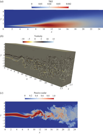
In this section, the DNS data for the planar jet flow are presented and compared with experimental and other reference simulation data from the literature. Additional data for the balance of the terms in the turbulent kinetic energy equation and the one-dimensional spectra of turbulent fluctuations are given in Appendix A. The turbulent kinetic energy,  $k$, in the (
 $x$–
 $y$) plane is depicted in figure 1(a) (because of symmetry, only the top half is shown). The jet breaks up at
 $x \approx 7.5$, and downstream of this location the turbulent kinetic energy rapidly grows and decays again; the maximum of
 $k$ is located at
 $(x,y)=(11,0.7)$. Contours of instantaneous spanwise vorticity and passive scalar fields,
 $\omega _z$ and
 $\phi$, are shown in figures 1(b) and 1(c), respectively. A downstream region with intense turbulent mixing and a wide range of turbulence length scales is evident.
Flow field data: (a) turbulent kinetic energy (TKE)  $k$; (b) 3-D view of the instantaneous spanwise vorticity field
 $\omega _z$; (c) instantaneous contours of the passive scalar on (
 $x$–
 $y$) plane
 $z=0$.

The growth of the jet half-width based on the streamwise velocity,  $\delta _U$, is shown in figure 2(a). The jet half-width
 $\delta _U$ is defined as the distance from the symmetry plane (centreline) to the point in the cross-stream direction where the mean streamwise velocity excess with respect to the co-flow velocity,
 $U_e(x,y) = U(x,y)-U_\infty (x)$, is half that with respect to the centreline,
 $\Delta U_c(x) = U_c(x) - U_\infty (x)$. The ratio of the velocity excess at the jet nozzle exit,
 $\Delta U_o = U_o - U_\infty$, to
 $\Delta U_c(x)$ is shown in figure 2(b).
Growth of the jet half-width based on the velocity (a) and centreline mean velocity excess decay (b). Blue line, present results;  $\Box$, Thomas & Chu (Reference Thomas and Chu1989);
 $\diamond$, Browne et al. (Reference Browne, Antonia, Rajagopalan and Chambers1983); dotted line, DNS (Stanley et al. Reference Stanley, Sarkar and Mellado González2002).

The growth of the jet half-width based on the passive scalar,  $\delta _\phi$, is shown in figure 3(a). The half-width
 $\delta _\phi$ is defined (similarly to
 $\delta _U$) as the distance from the symmetry plane (centreline) to the point where the passive scalar concentration is half of that on the centreline. The mean scalar decay, defined as
 $(\phi _o/\phi _c)^2$, where
 $\phi _c(x)$ is the value at the centreline and
 $\phi _o$ is the value at the jet nozzle exit, is shown in figure 3(b).
Downstream growth of the jet half-width based on the passive scalar (a) and decay of the mean scalar on the jet centreline (b). Blue line, present results;  $\diamond$, Browne et al. (Reference Browne, Antonia, Rajagopalan and Chambers1983);
 $\Box$, Davies, Keffer & Baines (Reference Davies, Keffer and Baines1975); dotted line, DNS (Stanley et al. Reference Stanley, Sarkar and Mellado González2002).

It can be seen that there is good agreement with the experimental and other reference data. Theoretical analysis (Rajaratnam Reference Rajaratnam1976; Pope Reference Pope2000) suggests that  $\delta _U \propto x$ and
 $U_c \propto 1/\sqrt {x}$ for planar jet flow, and the same scaling is also valid for the scalar concentration. It has been documented (Stanley & Sarkar Reference Stanley and Sarkar2000; Stanley et al. Reference Stanley, Sarkar and Mellado González2002; da Silva, Lopes & Raman Reference da Silva, Lopes and Raman2015) that the jet break-up location is highly affected by the inlet conditions at the nozzle. The jet characteristics are also affected by the value of the Reynolds number in cases where
 $Re<10\,000$ (Klein et al. Reference Klein, Sadiki and Janicka2003b; Deo, Mi & Nathan Reference Deo, Mi and Nathan2008). Therefore, independently of the exact location of the jet break-up, the slope of the curves shown in figures 2 and 3 for the present DNS exhibits good agreement with that of reference data.
The self-similar cross-stream profiles for velocity and scalar are depicted in figures 4(a) and 4(b), respectively. The velocity profiles collapse to a single curve, and there is good agreement with reference (experimental or other DNS) data. The velocity field reaches self-similarity at  $x \approx 12$, while the passive scalar is slightly slower to develop and the self-similar region is reached at
 $x \approx 17$. The same behaviour was also observed by Stanley et al. (Reference Stanley, Sarkar and Mellado González2002).
Self-similar profiles of mean velocity and mean passive scalar for three axial positions. (a) Mean velocity: solid lines, present results;  $\Box$, Gutmark & Wygnanski (Reference Gutmark and Wygnanski1976);
 $\circ$, Ramaprian & Chandrasekhara (Reference Ramaprian and Chandrasekhara1985); dotted line, DNS (Stanley et al. Reference Stanley, Sarkar and Mellado González2002). (b) Mean scalar: solid lines, present results;
 $\Box$, Davies et al. (Reference Davies, Keffer and Baines1975);
 $\circ$, Jenkins & Goldschmidt (Reference Jenkins and Goldschmidt1973); dotted line, DNS (Stanley et al. Reference Stanley, Sarkar and Mellado González2002).

3.2. Particle size distribution
The DNS–PBE approach allows for the prediction of the PSD at every point in the domain. As mentioned in § 2.1, in a perfectly stirred reactor, the PSD reaches a self-preserving distribution. Figure 5 shows the time-averaged PSDs at five different probe points on the centreline for both  $Da_{coag}$ number cases. The computed distributions are scaled according to (2.9) and (2.10), and compared with the self-preserving PSD from Vemury & Pratsinis (Reference Vemury and Pratsinis1995). It can be seen that as the PSDs develop, they approach the self-preserving distribution and there is good agreement with the reference data, especially close to the exit of the domain. Turbulence may affect the time to reach the self-preserving state (Friedlander Reference Friedlander2000). As mentioned earlier, the values of
 $Da_{coag}$ were chosen in such a way that the PSD becomes self-preserving before and after the jet break-up location for the two cases. In particular, for the
 $Da_{coag}=1/3$ case, the PSD becomes self-preserving slightly downstream of the expected location (
 $x \approx 15$). However, the difference observed is small. The fact that the PSDs in the turbulent flow field do not deviate a lot from the self-preserving distribution can be attributed to the lack of recirculating flow structures that would bring into contact particles with different distributions and would make the PSD deviate from the self-preserving state. Finally, the good matching with the reference data indicates that the number and distribution of volume intervals are sufficient to resolve the PSD accurately.
Normalised time-averaged PSDs at several probe points along the centreline. The results are compared with reference data for the self-preserving distribution (Vemury & Pratsinis Reference Vemury and Pratsinis1995). A logarithmic scale was used for the horizontal axes. (a)  $Da_{coag}=1$; (b)
 $Da_{coag}=1/3$.

4. Results and discussion
4.1. Effect of coagulation and mixing on the moments
The evolution of the moments is dominated by two physical mechanisms, coagulation and turbulent mixing, and by their interaction. Coagulation reduces the total number of particles,  $M_0$, with increasing distance from the orifice, but it does not alter the total particle volume,
 $M_1$, which behaves as a passive scalar. It also brings about an increase in the second moment,
 $M_2$, due to the heavier weighting of the large particles on the distribution. Turbulent mixing brings about dilution, which can be quantified using
 $M_1$.
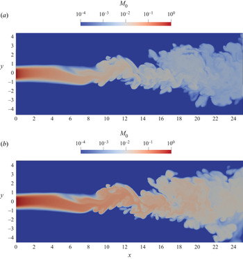
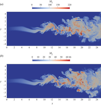
The instantaneous  $M_0$ fields for the two
 $Da_{coag}$ cases are depicted in figures 6(a) and 6(b), while the instantaneous
 $M_2$ fields are shown in figures 7(a) and 7(b). It is evident that
 $M_0$ reduces at downstream locations. The second moment,
 $M_2$, attains small values close to the jet nozzle and increases rapidly due to coagulation until the jet break-up location. The jet becomes unstable and breaks into smaller vortices, while the entrainment of co-flow fluid dilutes the large values of
 $M_2$. However, as can be seen, for example, in figure 7(a), the remnants of the core of the jet (see region
 $14< x<22$) are fluid patches with large values of
 $M_2$. Further downstream, the small-scale motion due to the strong turbulence in the jet has mixed further the fluid patches of the jet core. However, it is evident that
 $M_0$ reduces quite fast, while fluid patches with large values of
 $M_2$ start to emerge.
Instantaneous contour plots of  $M_0$ on (
 $x$–
 $y$) plane
 $z=0$. (a)
 $Da_{coag} = 1$; (b)
 $Da_{coag} = 1/3$. A logarithmic scale colourbar is used.

Instantaneous contour plots of  $M_2$ on (
 $x$–
 $y$) plane
 $z=0$.(a)
 $Da_{coag} = 1$; (b)
 $Da_{coag} = 1/3$.

The evolution of the zeroth moment,  $M_0$, is governed by the following equation in non-dimensional form, derived from (2.8) for
 $k=0$:
 \begin{equation} \frac{\partial M_0}{\partial t}+u_j\,\frac{\partial M_0}{\partial x_j} = \frac{1}{Sc}\,\frac{1}{Re}\,\frac{\partial^2 M_0}{{\partial x_j}\,{\partial x_j}} - \frac{1}{2} Da_{coag} \int_0^\infty \int_0^\infty \beta(v,w)\,n(v)\,n(w)\,{\rm d}v\,{\rm d}w. \end{equation}
The source term is negative because coagulation results in a reduction in the total number of particles. Figure 8(a) shows the centreline variation of the time-averaged  $\overline {M_0}$, juxtaposed with
 $\overline {M_1}$. There is a rapid reduction of the particle number concentration close to the jet nozzle, and the rate is higher for the higher
 $Da_{coag}$; this is expected because higher
 $Da_{coag}$ represents more intense coagulation. Both curves start to change behaviour at
 $x \approx 7.5$, where the jet breaks up and turbulent mixing starts to play an important role. From figure 8(a) it is evident that the rate of reduction (slope) of
 $\overline {M_0}$ is larger than that of
 $\overline {M_1}$ in the region of fully developed turbulence
 $(x>15)$. Dilutions due to turbulent mixing and coagulation work in unison and result in a reduction of
 $M_0$. The contribution of each mechanism can be quantified as follows. In the case of
 $Da_{coag}=1$,
 $\overline {M_0}$ is reduced by
 $89\,\%$ between the jet break-up location and the exit of the domain, while a passive scalar, such as
 $\overline {M_1}$, is reduced by
 $58\,\%$. Similarly, in the case of
 $Da_{coag}=1/3$,
 $\overline {M_0}$ is reduced by
 $88\,\%$ between the same locations. This indicates that both effects contribute to the evolution of
 $\overline {M_0}$, with turbulent dilution (rather than coagulation) having a slightly stronger effect.
Centreline variation of time-averaged  $M_0$ (a) and
 $M_2$ (b) for the two
 $Da_{coag}$ cases. The red dashed-dotted line indicates the jet break-up location. A logarithmic scale was used for the vertical axis in (a). A black dashed-dotted line is used for
 $\overline {M_1}$ in (a).

The transport equation for the second moment,  $M_2$, is derived from (2.8) for
 $k=2$:
 \begin{equation} \frac{\partial M_2}{\partial t}+u_j\,\frac{\partial M_2}{\partial x_j} = \frac{1}{Sc}\,\frac{1}{Re}\,\frac{\partial^2 M_2}{{\partial x_j}\,{\partial x_j}} + Da_{coag} \int_0^\infty \int_0^\infty v w \, \beta(v,w)\,n(v)\,n(w)\,{\rm d}v\,{\rm d}w. \end{equation}
For this moment, the source term is positive. Figure 8(b) shows the centreline variation of the time-averaged  $\overline {M_2}$. Unlike
 $M_0$, in the case of
 $M_2$ there is competition between dilution and coagulation. Turbulent mixing acts towards reducing
 $M_2$, while coagulation acts towards increasing
 $M_2$. As can be seen in figure 8(b), the net result is an increase in
 $M_2$. The effect of turbulence is thus to mitigate the rapid growth of the second moment. The net increase of
 $\overline {M_2}$ with distance after the jet break-up location indicates that coagulation has a greater effect on the evolution of
 $M_2$ compared to dilution.
4.2. Coagulation source term correlations
We now turn our attention to the effect of turbulent fluctuations and consider the Reynolds decomposition of the PBE (Scott Reference Scott1967; Friedlander Reference Friedlander2000; Rigopoulos Reference Rigopoulos2007). Apart from velocities, the number densities are also decomposed into mean and fluctuating parts, and this decomposition is substituted into (2.4). Time-averaging results in the equation
 \begin{align} &\bar{u}_j\,\frac{\partial \bar{n}}{\partial x_j} {+\frac{\partial \overline{u_j'n'}}{\partial x_j}} = \frac{1}{Sc}\, \frac{1}{Re}\,\frac{\partial^2 \bar{n}}{\partial x_j\,\partial x_j} \nonumber\\ &\quad+ Da_{coag} \left( \frac{1}{2} \int_0^v \beta(w,v-w)\,\bar{n}(w)\,\bar{n}(v-w)\,{\rm d}w - \int_0^\infty \beta(v,w)\,\bar{n}(v)\,\bar{n}(w) \,{\rm d}w \right. \nonumber\\ &\quad\left. + \frac{1}{2} \int_0^v \beta(w,v-w)\,\overline{n'(w)\,n'(v-w)}\,{\rm d}w - \int_0^\infty \beta(v,w)\,\overline{n'(v)\,n'(w)}\,{\rm d}w \right). \end{align}
The time-averaging of the transient term in (2.4) is zero for jet flow cases where statistical stationarity is reached. The last two terms arise due to turbulent coagulation; both involve integrals of correlations between number density fluctuations and are unclosed. Lack of understanding of the behaviour of correlations  $\overline {n'(v)\,n'(w)}$ is a long-standing problem in the literature (Levin & Sedunov Reference Levin and Sedunov1966, Reference Levin and Sedunov1968; Scott Reference Scott1967; Warshaw Reference Warshaw1967; Drake Reference Drake and Hidy1972).
The Reynolds decomposition can also be applied to the transport equation of moments, (2.8), resulting in
 \begin{align} \bar{u}_j\,\frac{\partial \overline{M_k}}{\partial x_j} + \frac{\partial \overline{u_j' M_k'}}{\partial x_j} &= \frac{1}{Sc}\,\frac{1}{Re}\,\frac{\partial^2 \overline{M_k}}{\partial x_j\,\partial x_j} \nonumber\\ &\quad + Da_{coag} \left( \frac{1}{2} \int_0^\infty \int_0^\infty (v+w)^k\,\beta(v,w)\, \bar{n}(v)\,\bar{n}(w)\,{\rm d}v\,{\rm d}w \right. \nonumber\\ &\quad - \frac{1}{2} \int_0^\infty \int_0^\infty (v^k+w^k)\,\beta(v,w)\, \bar{n}(v)\,\bar{n}(w) \,{\rm d}v\,{\rm d}w \nonumber\\ &\quad + \frac{1}{2} \int_0^\infty \int_0^\infty (v+w)^k\, \beta(v,w)\,\overline{n'(v)\,n'(w)}\,{\rm d}v\,{\rm d}w \nonumber\\ &\quad \left. - \frac{1}{2} \int_0^\infty \int_0^\infty (v^k+w^k)\,\beta(v,w)\,\overline{n'(v)\, n'(w)}\,{\rm d}v\,{\rm d}w \right). \end{align}
Similarly to the transport equation for the number density, the last two terms are unclosed. Analysis of these terms is important since the moments are measured frequently in experiments, and also a family of numerical methods for modelling particulate flows is based on the method of moments. Our analysis will focus on the unclosed terms in the transport equations of  $\overline {M_0}$ and
 $\overline {M_2}$ (coagulation does not alter
 $\overline {M_1}$, as already mentioned). Knowledge of these moments is also required in order to characterise the particle field with the method of moments when a log-normal size distribution is assumed (Brock, Kuhn & Zehavi Reference Brock, Kuhn and Zehavi1986).
As was mentioned in § 2.3, 35 intervals  $\Delta v_i$ were used to discretise the particle volume space
 $v$, thus for each computational cell there are
 $35 \times 35$ correlations
 $\overline {n'_i \, n'_j}$. As this is a very large amount of information, maps are presented for only a few points of interest in the domain. Results for the number density fluctuation correlations
 $\overline {n'(v)\,n'(w)}$ for the two values of
 $Da_{coag}$ at points
 $(x,y,z) = (10, 0, 0)$ and
 $(17.5, 0.5, 0)$ are shown in figure 9. The first point is located on the centreline and relatively close to the jet break-up location (
 $x \approx 7.5$), while the second point is further downstream, in the region of fully developed turbulence and slightly off the centreline. The results are presented in the form of contour maps with non-uniform spacing because of the exponential grid employed for the discretisation of the particle volume space. The map of the time-averaged number density combinations
 $\overline {n(v)} \, \overline {n(w)}$ for
 $Da_{coag}=1$ at probe point
 $(10, 0, 0)$ is also shown in figure 10(a). As expected, the maps are symmetric with respect to the diagonal
 $v = w$. For most of the points examined, it is found that the magnitude of
 $\overline {n'(v) \, n'(w)}$ follows that of
 $\overline {n(v)} \, \overline {n(w)}$, as can be seen in figures 9(a) and 10(a). More specifically, the maximum value of the correlation is found along the diagonal
 $v = w$ and close to the interval where
 $\bar {n}(v)$ has a local maximum, which is at the same interval where
 $\overline {n(v)} \, \overline {n(w)}$ receives the maximum value. For instance, the PSD at probe point
 $(10, 0, 0)$ for
 $Da_{coag}=1$, shown in figure 10(b), has a local maximum for
 $v \approx 5$ (in terms of discretised PBE, this corresponds to the third interval,
 $\overline {n_3}$), while the maximum value of the correlations at the same probe point were found for
 $(v, w) \approx (7.1,7.1)$ (see figure 10a). Furthermore, for large values of
 $v$ and
 $w$,
 $\overline {n'(v) \, n'(w)}$ tends to zero. These values correspond to the right tail of the PSD, where the mean number density
 $\bar {n}(v)$ is small (there are few particles of large size, as seen in figure 10b).
Map of number density fluctuation correlations  $\overline {n'(v)\,n'(w)}$: (a) for
 $Da_{coag}=1$ at probe point
 $(10, 0, 0)$; (b) for
 $Da_{coag}=1$ at probe point
 $(17.5, 0.5, 0)$; (c) for
 $Da_{coag}=1/3$ at probe point
 $(10, 0, 0)$; (d) for
 $Da_{coag}=1/3$ at probe point
 $(17.5, 0.5, 0)$.

(a) Map of time-averaged number density combinations  $\overline {n(v)}\,\overline {n(w)}$; (b) time-averaged PSD for
 $Da_{coag}=1$ at probe point
 $(10, 0, 0)$.

The correlations  $\overline {n'(v) \, n'(w)}$ are found to be mostly positive for most
 $v,w$ combinations, as shown in figure 9. Since we are not considering differential diffusion of particles of different sizes, the distribution is affected as a whole by turbulence, and coagulation is not rapid enough to redistribute fluctuations in a way that generates negative correlations, with the exception discussed below.
Negative values of the correlations  $\overline {n'(v) \, n'(w)}$ can also appear. This can be seen, for example, in figure 9(a) for
 $Da_{coag}=1$ at probe point
 $(10,0,0)$. These negative values involve mainly the fluctuation of the number density of the first interval,
 $n'_1$, and that of intervals that are on and to the right of the local maximum of
 $\bar {n}(v)$ (see figure 10b), e.g. the correlations
 $\overline {n'_1 \, n'_3}$ and
 $\overline {n'_1 \, n'_4}$ etc. A possible explanation for this effect is that at the inlet, only
 $n_1$ is non-zero, and coagulation acts towards reducing the instantaneous values of
 $n_1$ and increasing those of
 $n_2$,
 $n_3$, etc. A general trend is that the effect of coagulation is to move the distribution to the right in particle volume space towards higher particle volumes. For example, at probe point
 $(10,0,0)$, on average, coagulation acts towards reducing the instantaneous values of
 $n_1$ and increasing those of intervals at the right of the local maximum of
 $\bar {n}(v)$, such as
 $n_4$ (see figure 10b). Therefore, negative fluctuations of
 $n'_1$, in that case, are correlated with positive fluctuations of
 $n'_4$ and vice versa (when
 $n_1$ is consumed,
 $n_4$ is created). Once coagulation has progressed and the consumption of
 $n_1$ is not so intense, the correlations become positive. This also partly explains why negative correlations are found only for the case of intense coagulation (
 $Da_{coag}=1$) and for points close to the jet break-up location (
 $x<12.5$). Data for the downstream location
 $(17.5, 0.5, 0)$ are presented in figure 9(b), and it is observed that
 $\overline {n'(v) \, n'(w)} > 0$ for all combinations of
 $(v,w)$. Negative correlations are not found for the case
 $Da_{coag}=1/3$ (see also figures 9c,d). This means that
 $n_1'$ and
 $n_i'$ have the same sign probably because of the increased effect of turbulent mixing compared to the effect of coagulation.
It is of interest to examine the value of  $\overline {n'(v) \, n'(w)}$ in relation to the value of
 $\overline {n(v) \, n(w)}$. The intensity of the correlations of the number density fluctuations, the square of the passive scalar fluctuation intensity and the turbulence intensity are defined, respectively, as
 \begin{equation} I_n=\frac{\overline{n'(v) \, n'(w)}}{\overline{n(v) \, n(w)}} , \quad I_{\phi} = \frac{\overline{\phi'^2}}{\overline{\phi^2}}, \quad I_u = \frac{\overline{u_i'^2}}{\overline{U_i^2}}, \end{equation}
where  $I_u$ is defined here for future reference. Figure 11 shows a surface plot of
 $I_n$ at the probe point
 $(10, 0, 0)$ for the two
 $Da_{coag}$ cases. Here,
 $I_n$ is normalised with the value of
 $I_{\phi }$ at that specific location, while the location where the fluctuation intensities are equal (
 $I_n = I_{\phi }$) is also shown. First, note that the negative correlations referred to above can be seen very clearly in this plot. The differences with
 $I_{\phi }$ are small for the combinations
 $(v,w)$ of interest, i.e. the ones that make a large contribution to the integral. The value of
 $I_n$ increases as we move towards diagonal points with increasing
 $v$ and
 $w$, due to the fact that both the numerator and the denominator approach zero at these points. However, these points make a small contribution to the coagulation source term.
Intensity of correlations of number density fluctuations  $I_n$ at probe point
 $(10, 0, 0)$: (a)
 $Da_{coag} =1$; (b)
 $Da_{coag} =1/3$. Results are normalised by
 $I_{\phi }=0.156$. The black dashed line indicates the location where the fluctuation intensities are equal, i.e.
 $I_n = I_{\phi }$.

4.2.1. Effect of fluctuations on the zeroth moment
The transport equation for the time-averaged zeroth moment,  $\overline {M_0}$, is obtained from (4.4) for
 $k=0$ as
 $$\begin{gather} \bar{u}_j\,\frac{\partial \overline{M_0}}{\partial x_j} + \frac{\partial \overline{u_j' M_0'}}{\partial x_j} = \frac{1}{Sc}\,\frac{1}{Re}\,\frac{\partial^2 \overline{M_0}}{\partial x_j\,\partial x_j} + Da_{coag} \left( - \frac{1}{2} \int_0^\infty \int_0^\infty \beta(v,w)\,\bar{n}(v)\,\bar{n}(w) \,{\rm d}v\,{\rm d}w \right.\nonumber\\ \left. - \frac{1}{2} \int_0^\infty \int_0^\infty \beta(v,w)\,\overline{n'(v)\, n'(w)}\,{\rm d}v\,{\rm d}w \right). \end{gather}$$
In this section, we focus on the correlations arising from the Reynolds decomposition of the coagulation source term. This decomposition is shown below, with the terms labelled as  $A_0$,
 $B_0$ and
 $C_0$ to facilitate the subsequent discussion:
 $$\begin{gather} \underbrace{ -\frac{1}{2} \int_0^\infty \int_0^\infty \beta(v,w)\,\overline{n(v)\,n(w)}\,{\rm d}v\,{\rm d}w }_{A_0} = \underbrace{-\frac{1}{2} \int_0^\infty \int_0^\infty \beta(v,w)\, \bar{n}(v)\,\bar{n}(w)\,{\rm d}v\,{\rm d}w}_{B_0} \nonumber\\ \underbrace{- \frac{1}{2} \int_0^\infty \int_0^\infty \beta(v,w)\,\overline{n'(v)\,n'(w)}\,{\rm d}v\,{\rm d}w}_{C_0}. \end{gather}$$
A contour plot of the absolute values of  $A_0$ and a contour plot of
 $C_0$ for
 $Da_{coag}=1/3$ are depicted in figures 12(a) and 12(b), respectively (because of to symmetry, only the top half is shown). The term
 $C_0$ is unclosed and is usually neglected in studies of turbulent coagulation;
 $C_0$ attains the maximum value close to the orifice and in particular at the shear layer between the jet stream with the co-flow stream. In this region, Kelvin–Helmholtz instabilities develop, leading to vortical structures, and also the magnitude of the coagulation source term of the
 $M_0$ equation is very large close to the inlet. An important observation is that
 $C_0$ is negative everywhere in the domain, because for most
 $v,w$ combinations, the correlations
 $\overline {n'(v)\, n'(w)}$ were found to be positive, as was discussed before and shown in figure 9. The fact that
 $C_0 < 0$ means that, by neglecting it, one would overestimate
 $\overline {M_0}$. Qualitatively, this is also in agreement with the results of Garrick (Reference Garrick2011), where it was found that the predominant effect of the SGS contribution is to reduce particle growth.
Contour plots of  $|A_0|$ (a) and
 $C_0$ (b) for
 $Da_{coag}=1/3$. A logarithmic scale colourbar was used in (a).

The evolution of  $A_0$ for both
 $Da_{coag}$ numbers is depicted in figure 13. Solid lines were used for the case of
 $Da_{coag}=1$, and dashed lines for
 $Da_{coag}=1/3$. The values of
 $A_0$ along the centreline are shown in figure 13(a), where a logarithmic scale was used for the
 $y$ axis. It is observed that
 $A_0$ is larger in magnitude for the low
 $Da_{coag}$ case, and its values cover a range of four orders of magnitude. Close to the inlet, similarly to
 $\overline {M_0}$,
 $A_0$ attains the highest magnitude, which is
 $O(1)$. This is a region of rapid coagulation due to the high particle concentration. The value of
 $A_0$ drops rapidly with the distance from the orifice and eventually takes values that are
 $O(10^{-5})$ close to the outlet.
Coagulation source terms for the zeroth moment (see (4.7)). (a) Centreline values of  $A_0$; the red dashed-dotted line indicates the jet break-up location. (b) Cross-stream profiles of
 $A_0$,
 $B_0$ and
 $C_0$ at the axial position
 $x=20$. A logarithmic scale was used for the vertical axis in (a). The horizontal axis in (b) was normalised by
 $\delta _{\phi }=2.362$. Note the different horizontal axes in (a) and (b).

The cross-stream profiles at the axial position  $x=20$ – where self-similarity is verified by both simulations – of each term in (4.7) are shown in figure 13(b). It is observed that the maximum magnitude of
 $C_0$ is not found on the centreline. Specifically,
 $C_0$ increases as we move from the centreline to the jet edges, reaches its maximum value, and then decreases. This picture is consistent with the contour plot shown in figure 12. This behaviour is similar to that found for the TKE and the passive scalar fluctuations
 $\sqrt {\overline {\phi '^2}}$ profiles. The horizontal axes in figures 13(b) and 14(b) are non-dimensionalised with
 $\delta _\phi =2.362$ (the jet half-width based on the passive scalar for the axial position
 $x=20$).
To elucidate further the effect of turbulent fluctuations on coagulation, the relative contribution of each term on the right-hand side of (4.7) is examined. Here,  $C_0$ is normalised by
 $A_0$, and the results along the centreline for both
 $Da_{coag}$ values are shown in figure 14(a). The ratio
 $C_0/A_0$ represents the contribution of the number density fluctuations to the total coagulation source term. It can also be seen that
 $C_0/A_0$ seems to have a weak dependence on
 $Da_{coag}$ (figures 14a,b). The centreline values of
 $C_0/A_0$ are zero close to the inlet. The ratio starts to increase after the jet break-up, and reaches the value
 $18\,\%$ at
 $x=12.4$. After this point, the ratio gradually decreases and reaches the value
 $5\,\%$ at the exit of the computational domain. It can be seen that at the centreline,
 $C_0$ makes a significant contribution (approximately 20 %) to the mean source term
 $A_0$.
 $C_0/A_0$ ratio (see (4.7)). (a) Centreline values of
 $C_0/A_0$. (b) Cross-stream profiles of
 $C_0/A_0$ at the axial position
 $x=20$. The horizontal axis in (b) was normalised by
 $\delta _{\phi }=2.362$. Note the different horizontal axes in (a) and (b).

This contribution increases close to the jet edges, as shown by the cross-stream profiles of  $C_0/A_0$ plotted in figure 14(b) for
 $x=20$ for both
 $Da_{coag}$ cases. For example, at
 ${y/\delta _\phi =1}$, the ratio
 $C_0/A_0$ has values between 30 % and 40 %. In other words, as the jet spreads, the difference between
 $B_0$ and
 $A_0$ increases, and at the point where the value of the first moment
 $(M_1 \equiv \phi )$ has dropped to half of the value on the centreline, the difference has reached a value between 30 % and 40 %. Further away from the centreline, both
 $A_0$ and
 $C_0$ assume very small values and therefore no significance can be ascribed to their ratio, which approaches 1 as
 $C_0/A_0 = 1 - B_0/A_0$ and
 $B_0$ approaches zero. The same behaviour was also found for
 $I_{\phi }$. Nevertheless, the region far away from the centreline is not of interest, since the number concentration of particles is also very small. From this discussion, it can be concluded that
 $C_0$ should not be neglected in the modelling of turbulent coagulation.
For comparison purposes, the squares of the passive scalar fluctuations intensity,  $I_{\phi }$, and the velocity fluctuations intensity,
 $I_u$, are also shown in figure 14. An interesting observation is that
 $C_0/A_0$ has qualitatively and quantitatively the same behaviour as
 $I_{\phi }$. Dilution due to turbulent mixing (rather than coagulation) was found to have a slightly greater effect on the evolution of
 $M_0$, as was discussed in § 4.1. This partly explains why
 $C_0/A_0$ behaves like
 $I_{\phi }$.
4.2.2. Effect of fluctuations on the second moment
The analysis of the previous section is now performed for the second moment. The transport equation of  $\overline {M_2}$ can be derived by setting
 $k=2$ into (4.4), which results in
 $$\begin{gather} \bar{u}_j\,\frac{\partial \overline{M_2}}{\partial x_j} {+ \frac{\partial \overline{u_j' M_2'}}{\partial x_j}} = \frac{1}{Sc}\,\frac{1}{Re}\,\frac{\partial^2 \overline{M_2} }{\partial x_j\,\partial x_j} + Da_{coag} \left( \int_0^\infty \int_0^\infty v w \, \beta(v,w)\,\bar{n}(v)\,\bar{n}(w) \,{\rm d}v\,{\rm d}w\right.\nonumber\\ \left.+ \int_0^\infty \int_0^\infty v w \, \beta(v,w)\,\overline{n'(v)\,n'(w)}\,{\rm d}v\,{\rm d}w \right). \end{gather}$$
The correlations arising from the Reynolds decomposition of the coagulation source term are labelled as follows:
 $$\begin{gather} \underbrace{ \int_0^\infty \int_0^\infty v w \, \beta(v,w)\,\overline{n(v)\,n(w)}\,{\rm d}v\,{\rm d}w}_{A_2} = \underbrace{\int_0^\infty \int_0^\infty v w \, \beta(v,w)\,\bar{n}(v)\,\bar{n}(w)\,{\rm d}v\,{\rm d}w}_{B_2} \nonumber\\ + \underbrace{ { \int_0^\infty \int_0^\infty v w \, \beta(v,w)\,\overline{n'(v)\,n'(w)}\,{\rm d}v\,{\rm d}w}}_{C_2}. \end{gather}$$
The evolution of  $A_2$ and
 $C_2$ for
 $Da_{coag}=1/3$ is shown in figure 15. The value of the term
 $C_2$ is positive everywhere in the domain, again because
 $\overline {n'(v)\,n'(w)}$ is mostly positive, as discussed before. This implies that neglecting
 $C_2$ would lead to an underestimation of
 $\overline {M_2}$. Figure 15(b) shows that away from the centreline towards the jet edges,
 $C_2$ increases until reaching a local maximum, at roughly
 $(x,y)=(9,0.55)$ for both runs, and then drops to zero. The maximum is located slightly downstream of the jet break-up and coincides with the location where the r.m.s. value of the passive scalar fluctuations
 $\sqrt {\overline {{\phi '}^2}}$ is maximised. For reference, the location of the maximum TKE is
 $(x,y)=(11,0.7)$.
Contour plots of  $A_2$ (a) and
 $C_2$ (b) for
 $Da_{coag}=1/3$.

The variation of  $A_2$ in the centreline is shown in figure 16(a) for both
 $Da_{coag}$ numbers. In the absence of flow,
 $A_2$ would increase monotonically with time. Indeed, this is exactly what happens close to the jet nozzle;
 $A_2$ increases with distance away from the orifice (time can be converted easily to distance). Shortly upstream of the jet break-up location (red dashed-dotted line in figure 16a),
 $A_2$ starts to decrease and eventually reaches values smaller even than those at the inlet. The maximum of
 $C_2$ along the centreline is found at around
 $x=11$. The highest deviation between
 $A_2$ and
 $B_2$ is found in the region between
 $x=7.5$ and 18, and this is true for both
 $Da_{coag}$ numbers. It is also noted that even though
 $A_2$ is reduced, the effect of coagulation can compensate for the effect of turbulent dilution on mean
 $M_2$; this can be concluded from the fact that the latter increases in the streamwise direction, as shown in figure 8(b).
Coagulation source terms of the second moment equation (see (4.9)). (a) Centreline values of  $A_2$,
 $B_2$ and
 $C_2$; the red dashed-dotted line indicates the jet break-up location. (b) Centreline values of ratio
 $C_2/A_2$.

The variation of the ratio  $C_2/A_2$ along the centreline is depicted in figure 16(b). This ratio represents the relative contribution of the number density fluctuations to the total source term. Note that
 $C_2/A_2$ was found to have a weak dependence on
 $Da_{coag}$ for the cases examined, similar to
 $C_0/A_0$. The maximum along the centreline is
 $20.6\,\%$ and is found at
 $x=12.5$, while the peak value of
 $C_0/A_0$ was around
 $17.5\,\%$ found at the same location
 $x$. It can be seen that
 $C_2$ makes a large contribution to
 $A_2$ and therefore should not be neglected for accurate modelling of turbulent coagulation.
For comparison purposes, the squares of the passive scalar fluctuations intensity  $I_{\phi } = {\overline {{\phi '}^2}}/{\overline {\phi ^2}}$ and the velocity fluctuations intensity
 $I_u = {\overline {{{u_i}'}^2}}/{\overline {{U_i}^2}}$ are also shown in figure 16(b). An interesting observation is that
 $C_2/A_2$ reaches higher values than the ratio
 $C_0/A_0$. It was shown in § 4.2.1 that
 $C_0/A_0$ reaches values close to
 $I_{\phi }$ (see figure 14a). On the contrary, it is observed from figure 16(b) that the relative difference between the peak value of
 $C_2/A_2$ and that of
 $I_{\phi }$ is
 $18\,\%$. Coagulation was found to have a greater effect on the evolution of
 $M_2$ in this region, as discussed in § 4.1. This has to do with the heavier weighting of the large particles of the distribution, which are formed due to coagulation at downstream positions, on the second moment. On the other hand, turbulent dilution (rather than coagulation) was found to have a slightly stronger effect on the evolution of
 $M_0$. This partly explains why
 $C_2/A_2$ reaches higher values than the ratio
 $C_0/A_0$.
5. Conclusions
The objective of the present paper was to present a DNS study of turbulence–coagulation interaction. In particular, the study focused on the behaviour and significance of the unknown correlations of fluctuations that arise from the Reynolds decomposition of the PBE and moment transport equations. These correlations appear in any problem featuring turbulence and coagulation, such as soot formation and nanoparticle synthesis, but usually in conjunction with other physical and chemical effects, such as those associated with chemical kinetics. Hence the numerical experiments in the present study are intended to isolate the effect of turbulence–coagulation interaction. The numerical experiments were conducted in the Eulerian DNS–PBE framework, where the DNS resolves the flow down to the Kolmogorov scale, while the PBE is solved via a discretisation method that is free of a priori assumptions regarding the shape of the PSD. A unity Schmidt number was employed, as it is not feasible at present to resolve the Batchelor scales that result from diffusion at high Schmidt numbers. Direct numerical simulations of a 3-D turbulent planar jet flow at  $Re=3000$ were performed, for which it was feasible to obtain a fully resolved turbulent flow as well as an accurate numerical solution of the PBE in the whole domain, and the flow field was validated by comparison with reference experimental and DNS data. The jet was laden with monodispersed nanoparticles issued into a particle-free co-flow stream. The phenomena under investigation were turbulent mixing and particle coagulation in the free-molecule regime. Simulations for two different coagulation Damköhler numbers,
 $Da_{coag}=1$ and
 $1/3$, were carried out, where
 $Da_{coag}$ is defined as the ratio of a convection time scale to a coagulation time scale, the latter related to the time needed to reach the self-preserving distribution.
The correlations of the fluctuating number densities were calculated at specific probe points in the domain. It was found that the correlations were mostly positive for all combinations of particle volumes. However, negative correlations were also present for the case of more intense coagulation, i.e.  $Da_{coag}=1$, close to the jet break-up location. Furthermore, the intensity of the correlations was examined by normalising them with the mean of the product of the number densities. Results showed that the intensity maps have rather uniform values with magnitude close to the square of the passive scalar fluctuations intensity.
Unclosed terms also arise during the Reynolds decomposition of the transport equations for the zeroth and second moments. The unclosed terms make a large contribution to the time-averaged coagulation source terms and therefore should not be neglected. More specifically, for the transport equation of  $\overline {M_0}$, the ratio of the term with the unknown correlations (denoted
 $C_0$) to the time-averaged coagulation source term (denoted
 $A_0$) reaches values as high as
 $18\,\%$ on the jet centreline, and increases up to
 $40\,\%$ close to the jet edges. Furthermore, the value of
 $C_0$ was negative everywhere in the domain because, for most particle size combinations, the correlations of the fluctuating number densities were found to be positive. The negative value of
 $C_0$ indicates that neglect of
 $C_0$ could lead to an overestimation of
 $\overline {M_0}$. For the transport equation of
 $\overline {M_2}$, the ratio of the term with the unknown correlations (denoted
 $C_2$) to the time-averaged coagulation source term (denoted
 $A_2$) reached values as high as
 $20\,\%$ on the jet centreline, and the value of
 $C_2$ was positive everywhere in the domain.
In the present flow configuration, the ratio  $C_0/A_0$ showed the same behaviour as that of the square of the passive scalar fluctuations intensity. This indicates that dilution due to turbulent mixing (rather than coagulation) had a slightly greater effect on the evolution of
 $M_0$ in the region downstream of the jet break-up location. On the contrary,
 $C_2/A_2$ was found to reach higher values than
 $C_0/A_0$, with a relative difference of the peak values close to
 $18\,\%$, indicating that coagulation (rather than turbulent dilution) had a greater effect on the evolution of
 $M_2$. Finally, both ratios were found to have a weak dependence on the
 $Da_{coag}$ number, at least for the cases examined.
To summarise, the present study aimed to refine our understanding of the effect of turbulent fluctuations on the coagulation process. Coagulation is a key process in several engineering and environmental problems – including soot formation, flame synthesis of nanoparticles such as silica and titania, and atmospheric aerosols – and understanding its interaction with turbulence is important for developing judicious assumptions and developing accurate models for predicting particle-laden flows. Future work should examine these interactions within more complex flows and in situations where other particulate phenomena, such as nucleation and growth, are present.
Funding
The authors are grateful to the Leverhulme Trust for financial support (grant reference RPG-2018-101). The authors also wish to acknowledge the UK Consortium on Turbulent Reacting Flows (www.ukctrf.com) for providing access to the ARCHER facility through EPSRC grant EP/R029369/1, as well as the UK Materials and Molecular Modelling Hub for computational resources on THOMAS through EPSRC grant EP/P020194/1.
Declaration of interests
The authors report no conflict of interest.
Appendix A
The turbulent kinetic energy (TKE) equation takes the form (Pope Reference Pope2000)
 $$\begin{gather} \underbrace{ -\bar{u}_j\,\frac{\partial}{\partial x_j} \left( \frac{1}{2} \, \overline{u_i' u_i'} \right)}_{C_k} \underbrace{{}- \frac{\partial}{\partial x_j} \left( \frac{1}{\rho} \, \overline{u_j' p'} \right)}_{{\rm \pi}_k} \underbrace{{}- \frac{\partial}{\partial x_j} \left( \frac{1}{2} \overline{u_i' u_i' u_j'} \right) }_{T_k} \nonumber\\ \underbrace{{}+ \frac{\partial}{\partial x_j} \left( 2\nu \, \overline{u_i' \, s_{ij}} \right) }_{D_k} \underbrace{{}- \overline{u_i' u_j'}\,S_{ij} }_{P_k} \underbrace{{}- 2\nu \, \overline{s_{ij} \, s_{ij}}}_{\epsilon_k} = 0, \end{gather}$$
where  $S_{ij}$ and
 $s_{ij}$ denote the mean and fluctuating strain rates, respectively:
 \begin{equation} S_{ij} = \frac{1}{2} \left( \frac{\partial \bar{u}_i}{\partial x_j} + \frac{\partial \bar{u}_j}{\partial x_i} \right), \quad s_{ij} = \frac{1}{2} \left( \frac{\partial u_i'}{\partial x_j} + \frac{\partial u_j'}{\partial x_i} \right). \end{equation}
In (A1), terms  $C_k$,
 ${\rm \pi} _k$,
 $T_k$,
 $D_k$,
 $P_k$ and
 $\epsilon _k$ denote convection due to mean flow, pressure gradient work, transport by velocity fluctuations, viscous diffusion, production by mean flow, and dissipation, respectively. The variation of these terms together with their sum,
 $\varSigma$, along the jet centreline is shown in figure 17. Overall, the equation is well balanced, with the maximum error being less than
 $5.5\,\%$ of the peak absolute value of convection due to mean flow. This indicates that the resolution of the computational grid is fine enough.
Variation of turbulent kinetic energy budgets along the jet centreline (all terms are non-dimensionalised with the variables defined in (2.3a–d)).

Figure 18 shows the one-dimensional  $E_{11}(\kappa _1)$ and
 $E_{22}(\kappa _1)$ spectra of turbulent fluctuations, plotted with Kolmogorov scaling. For the definition of these quantities, we refer to Pope (Reference Pope2000). The spectra are presented as functions of streamwise wavenumber
 $\kappa _1$, and they were obtained from the frequency spectra of the streamwise and cross-stream velocity fluctuations at the probe point
 $(x,y,z) = (20,1.5,0)$, which is located in the region of fully developed turbulence. The conversion of the frequency to wavenumber spectra is based on Taylor's ‘frozen turbulence’ hypothesis (Taylor Reference Taylor1935) and was performed through the variable transformation
 $\kappa _1 = 2 {\rm \pi}f / U_c$, where
 $f$ is the frequency, and
 $U_c$ is a convection velocity taken as the time-averaged streamwise velocity at that probe point. The Kolmogorov
 $-5/3$ power-law one-dimensional spectra
 $E_{11}(\kappa _1) = C_1 \, \epsilon ^{2/3} \, \kappa _1^{-5/3}$ and
 $E_{22}(\kappa _1) = C_1' \, \epsilon ^{2/3} \, \kappa _1^{-5/3}$ were also calculated using the value of the turbulent kinetic energy dissipation rate at that probe point and presented in the figures for comparison. The values of the universal constants
 $C_1$ and
 $C_1'$ are
 $0.49$ and
 $0.65$, respectively (Pope Reference Pope2000). Although, for the flow conditions examined, an extended inertial region is not expected, the DNS data do exhibit a power-low close to
 $-5/3$ over about a decade, and match well the theoretical spectra. Furthermore, at high frequencies, a dissipative range with a faster decay rate is observed, which indicates that the turbulent motions are well resolved.
One-dimensional power spectra  $E_{11}(\kappa _1)$ (a) and
 $E_{22}(\kappa _1)$ (b) obtained from the frequency spectra of the streamwise and cross-stream velocity fluctuations at the probe point
 $(x,y,z) = (20,1.5,0)$. Kolmogorov's universal scaling was used. The dashed red lines represent the one-dimensional wavenumber spectra (a)
 $E_{11}(\kappa _1) = C_1 \, \epsilon ^{2/3} \, \kappa _1^{-5/3}$ and (b)
 $E_{22}(\kappa _1) = C_1' \, \epsilon ^{2/3} \, \kappa _1^{-5/3}$. Logarithmic scales were used for both axes.