2.1. Flow decomposition and asymptotic scalings

We consider ring-mode CS on a compressible axisymmetric circular jet, produced by an exhaust mean-flow velocity $U_{{I}}^*$ and a coflow $U_{{O}}^*$ with $U_{{I}}^* > U_{{O}}^*$, separated by a circular nozzle. The temperatures in these two streams are $T_{{I}}^*$ and $T_{{O}}^*$, respectively. The flow is to be described using cylindrical coordinates ($x, r, \theta$), with the corresponding velocity being denoted by $\pmb {u}=(u,v,w)$. The axial and radial coordinates, $x^*$ and $r^*$, and time $t^*$ are non-dimensionalised by $\delta _0^*$ and $\delta _0^*/U_0^*$, respectively, where the superscript $^*$ signifies a dimensional quantity, $\delta _0^*$ denotes the shear-layer thickness at a typical axial position, and $U_0^*$ is a reference velocity. The velocity $U^*$, density $\rho ^*$, temperature $T^*$ and viscosity $\mu ^*$ are normalised by

(2.1a–d)\begin{equation} U_0^*=(U_{{I}}^*-U_{{O}}^*)/2,\quad\rho_0^*=\rho_{{I}}^*,\quad T_0^*=T_{{I}}^*,\quad \mu_0^*=\mu_{{I}}^*, \end{equation}

respectively, while the non-dimensional pressure $p$ is introduced by writing

(2.2)\begin{equation} p^*=p_0^*+\rho_0^*U_0^{*2}p. \end{equation}

The resulting dimensionless parameters, including the Mach number ${Ma}$, the Reynolds number ${Re}$ and the Prandtl number $Pr$, are defined as

(2.3a–c)\begin{equation} {Ma}={U_0^*}/{\sqrt{\gamma R_g^* T_0^*}},\quad {Re}={\rho_0^*U_0^*\delta_0^*}/{\mu_0^*},\quad Pr={\mu_0^*C_p^*}/{k_0^*}, \end{equation}

where $R_g^*$ is the universal gas constant, $k_0^*$ is thermal conductivity, and $\gamma =C_p/C_v$ with $C_p$ and $C_v$ being the constant-pressure and constant-volume specific heat capacities, respectively. The Mach number of the exhaust flow, ${Ma}_{{I}}$, is for convenience defined as

(2.4)\begin{equation} {Ma}_{{I}}=\frac{2U_{{I}}^*}{U_{{I}}^*-U_{{O}}^*}{Ma}\mathop{=\!\!\!\!=\!\!\!\!=}\limits^{def.}\bar{U}_-{Ma}. \end{equation}

As in the planar cases (Wu & Zhuang Reference Wu and Zhuang2016; [I]), we adopt the triple decomposition (Hussain & Reynolds Reference Hussain and Reynolds1972)

(2.5)\begin{equation} (\pmb{u},T, p,\rho) = (\pmb{\bar{U}},\bar{T},\bar{P},\bar{\rho})+ (\pmb{\tilde{u}},\tilde{T},\tilde{p},\tilde{\rho})+ (\pmb{u}',T', p',\rho');\end{equation}

that is, the instantaneous field $(\pmb {u},T,p,\rho )$ is composed of the mean flow $(\pmb {\bar {U}},\bar {T},\bar {P},\bar {\rho })$, the quasi-periodic coherent motion $(\pmb {\tilde {u}},\tilde {T},\tilde {p},\tilde {\rho })$, and small-scale turbulence $(\pmb {u}',T', p',\rho ')$. The CS signature $\tilde {f}$ is obtained by $\tilde {f}\equiv \langle f\rangle -\bar {f}$, where the angle braces denote the (Favre) phase-averaging, and the over-bar indicates (Favre) time-averaging; see [I] for details.

The governing equations, together with the closure models for the time-averaged Reynolds stresses $\bar {\tau }_{ij}$ and the coherent Reynolds stresses $\tilde {\tau }_{ij}$, are the same as those in [I] once the operator $\partial _y\bullet$ is replaced by $r^{-1}\partial _r (r\bullet )$. Definitions for the parameters, such as $Pr_T$, $\widetilde {Pr}_T$, $R_T$, $\tilde {R}_T$, $\tilde {\mu }_t$, could be also found in (2.19)–(2.22) and (2.30)–(2.33) of [I]. There are also the time delays $\hat {\tau }_1$ and $\hat {\tau }_2$, introduced in the closure models, between the coherent Reynolds stresses and the strain rates of CS.

The turbulent Reynolds and Prandtl numbers, $R_T$ and $Pr_T=O(1)$, are introduced in the Reynolds-stress model for $\overline {u_i'u_j'}$, while the coherent Reynolds and Prandtl numbers, $\tilde {R}_T$ and $\widetilde {Pr}_T=O(1)$, arise through the coherent-Reynolds-stress model for 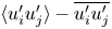$\langle u_i'u_j'\rangle -\overline {u_i'u_j'}$. It is assumed that ${Re}\gg R_T\gg 1$, which is reasonable since the eddy viscosities are much greater than the molecular viscosity (Wu & Zhuang Reference Wu and Zhuang2016; [I]). The axial development of the mean flow is described by the slow variable

(2.6)\begin{equation} \tilde{x}={x}/R_T.\end{equation}

The radial velocity scales as $R_T^{-1}\bar {V}$, with $\bar {V} =O(1)$, and the mean flow can be written as ($\bar {U}(\tilde {x},r)$, $R_T^{-1}\bar {V} (\tilde {x},r)$, $\bar {T}(\tilde {x},r)$, $\bar {P}$, $\bar {\rho }(\tilde {x},r)$). In this paper, we consider the full developed region of the jet, where the shear-layer thickness is comparable with the nozzle diameter $D^*$, i.e. $\delta _0^*=O(D^*)$, and the shear flow occupies the radial region where $r=O(1)$.

The dynamics of a ring-mode CS is similar to that of a two-dimensional instability mode considered in [I]. The region where the mode is nearly neutral is of special importance because the CS has acquired its maximum magnitude there and thus is prone to nonlinear effects in the critical layer (Wu Reference Wu2019). On a subsonic jet, the mean-flow temperature profile usually has a moderate radial gradient. By treating this gradient as a small quantity such that the major nonlinearity is associated with both the simple-pole singularity of the temperature disturbance and the logarithm singularity of the second term in the outer expansion of the axial velocity, the resulting critical-layer dynamics is strongly nonlinear, as explained in Sparks & Wu (Reference Sparks and Wu2008) and [I], and furthermore weakly nonlinear dynamics can be recovered as a limiting case. Let $\tilde {q}$ represent any of the velocity, temperature, pressure and density of the CS. Then in the main part of the flow, a ring-mode CS can, at leading order, be represented by a modulated travelling wave

(2.7)\begin{equation} \tilde{q} =\epsilon\,A^{\dagger}(\tau,\bar{x})\,\hat{q}(r)\,{\rm e}^{{\rm i}\alpha\zeta}+{\rm c.c.} ,\end{equation}

where $\zeta =x-ct$, with $\alpha =O(1)$, and $c=O(1)$ are the wavenumber and phase speed of the locally neutral mode, respectively, $\epsilon \ll 1$ is a measure of its magnitude, and $\hat {q}(r)$ characterises its radial distribution; the spatial–temporal modulation is described by the amplitude function $A^{\dagger}$ of the slow temporal and spatial variables $\tau$ and $\bar {x}$, defined as

(2.8a,b)\begin{equation} \tau= \epsilon^{1/2} t,\quad \bar{x}= \epsilon^{1/2} c^{{-}1} (x- R_T \tilde{x}_N), \end{equation}

for modulation taking place in the non-equilibrium nonlinear critical layer, where $\tilde {x}_N$ denotes the axial position where the mode becomes neutral. CS of such a wavepacket form consist of sideband spectral components adjacent to the fundamental wave, which are encapsulated in the envelope $A^{\dagger}$. The spatial–temporal modulation of the latter is crucial in the acoustic radiation, as will become clear later. With a narrow-band spectrum (centred at the frequency of the locally neutral mode), this wavepacket model represents of course only large-scale CS. A wavepacket will typically be taken to be a superposition of time-periodic disturbances (see § 3.2) and is in general quasi-periodic. Such a wavepacket represents fairly well CS generated by harmonic excitation. In an unforced jet, CS are excited by stochastic disturbances in the turbulent boundary layer on the nozzle wall and can also be educed (Zaman & Hussain Reference Zaman and Hussain1984), and the dominant CS, whose frequencies are close to that of the preferred mode, may also be represented by wavepackets, albeit with a somewhat broader sideband.

In order to include viscosity and non-parallelism along with nonlinear and non-equilibrium effects at the leading order in the dynamical system, the parameters ${Re}$, $\tilde {R}_T$ and $R_T$ are scaled as (Wu & Zhuang Reference Wu and Zhuang2016; [I])

(2.9a–c)\begin{equation} {Re}^{{-}1}=\bar{\lambda}\epsilon^{3/2},\quad \tilde{R}_T^{{-}1}=\tilde{\lambda}\epsilon^{3/2},\quad R_T^{{-}1}=\sigma \epsilon/c, \end{equation}

where $\bar {\lambda },\tilde {\lambda }= O(1)$ are Haberman (Reference Haberman1972) parameters, and $\sigma = O(1)$. It follows from (2.6) and (2.8a,b) that $\tilde {x}$ and $\bar {x}$ are related via $\tilde {x}=\tilde {x}_N+\epsilon ^{1/2}\sigma \bar {x}$.

The self-interaction of CS of strongly nonlinear nature takes place in the critical layer centred at $r_c$, where $\bar {U}(r_c)=c$. For a subsonic mode, the critical level $r_c$ is located at the generalised inflection point, where $({\partial }/{\partial r})\bar {\rho }({\partial \bar {U}}/{(r\,\partial r)})=0$. The dominant nonlinearity, driven by $\tilde {v}\partial _r\bullet$ according to scaling analysis, is required to balance the non-equilibrium effect, which suggests the appropriate transverse variable

(2.10)\begin{equation} Y={(r-r_c)}/{\epsilon^{1/2}}.\end{equation}

It is worth pointing out that in the developed region of the jet, $r_c=O(1)$. In the near-nozzle region, the jet consists of a potential core and a thin shear layer developing along the lip line, so $\delta _0^*\ll D^*$ while the critical level is located at $r^*\approx D^*/2$. It follows that $r_c\gg 1$. The size of $r_c^{-1}$ thus characterises different axial regions as $\delta _0^*/D^*$ does.

As will be shown, while the physical acoustic source is located in the main flow and the critical layer, the fluctuations acquire the character of sound waves in an outer acoustic region. Its radial extent is comparable with the axial length scale of the wavepacket envelope, so we introduce the acoustic transverse variable

(2.11)\begin{equation} \bar{r}={\epsilon^{1/2}{c^{{-}1}}r}.\end{equation}

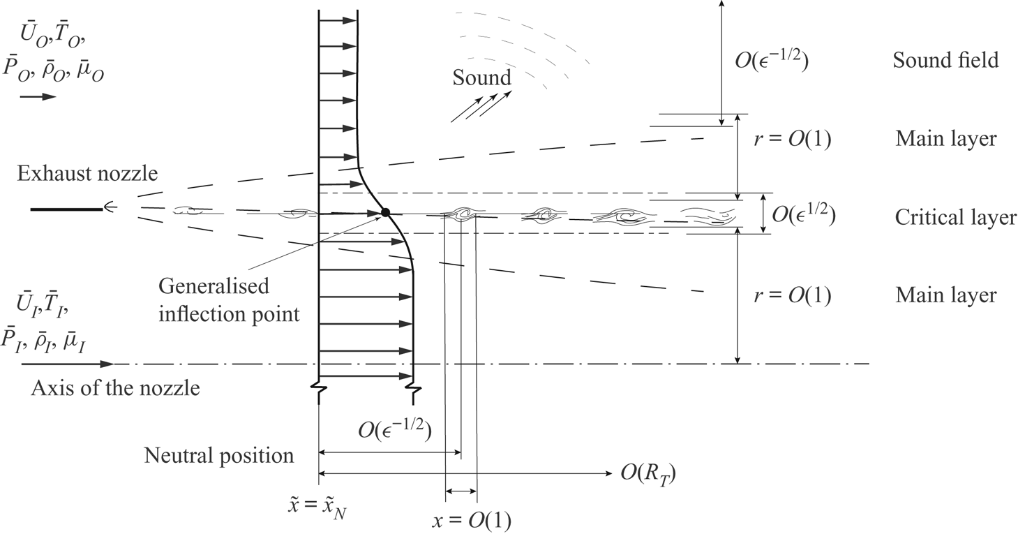
The overall asymptotic structure of the flow and the relevant asymptotic scalings are illustrated in figure 1. The three layers in the radial direction will be analysed in order to derive the nonlinear evolution system of the CS, and to determine the emitted sound waves. The ensuing analysis may appear rather complex, but the major steps and outcomes can be understood without going through all the details, and they are highlighted as follows. The main jet flow is considered first in § 2.2. The fundamental component of the CS appears at leading order as a nearly neutral instability mode governed by an eigenvalue problem. At the next order, an inhomogeneous Rayleigh equation arises, and its solvability condition leads to an ‘embryo amplitude equation’ (2.28), which contains a jump. The unsteady mean-flow distortion, induced by interactions in the main flow as well as in the critical layer, is analysed in § 2.3. The key outcome is (2.36), in which the forcing terms represent the physical sources in the main shear flow. The solution, given by (2.38), allows for a jump across the critical layer. The latter is considered in § 2.4 to derive the equations for the temperature and vorticity disturbance, (2.47) and (2.48), and the jump in the fundamental component is deduced and combined with (2.28) to obtain the amplitude equation (2.51). The resulting closed system, (2.47)–(2.48) with (2.51), governs the nonlinear development of the CS. Further analysis at a higher order determines the jump in the mean-flow distortion, (2.56), which is contributed by nonlinear interactions in the critical layer and represents another physical source of sound. The radial velocity decays in inverse proportion to the radial distance, indicating that the breathing mean flow acts an emitter with an equivalent source (2.57), which can be expressed in terms of the physical sources.

Figure 1.

Asymptotic structure of, and the scalings in, the axial and radial directions.

2.2. Disturbances in main shear flow and their far-field asymptote

Let $\tilde {q}$ represent any of $\tilde {u}$, $\tilde {v}$, $\tilde {T}$, $\tilde {p}$ and $\tilde {\rho }$, which are all quantities to describe the CS. In the main part of the jet, $\tilde {q}$ is expanded as an asymptotic series

(2.12)\begin{align} \tilde{q}(\tau,\bar{x},r,\zeta,\theta)=\epsilon\,A^{\dagger}(\tau,\bar{x})\,\hat{q}_0(r) \,{\rm e}^{{\rm i}\alpha\zeta} +\epsilon^{3/2}\sum_{n=1}^\infty \hat{q}_1^{\langle n\rangle}(\tau,\bar{x},r)\,{\rm e}^{{\rm i} n\alpha\zeta} +{\rm c.c.}+\cdots+\tilde{q}_M ,\end{align}

where $\tilde {q}_M$ stands for the slowly modulated mean-flow distortion, generated by nonlinear interactions of CS; it will be analysed in § 2.3. Inserting (2.12) into the CS equations (see [I]) at $O(\epsilon )$, we obtain the eigenvalue problem consisting of the homogeneous compressible Rayleigh equation for pressure $\hat {p}_0$ and the boundary condition

(2.13)\begin{equation} {\mathcal{L}}_R^{\langle 1\rangle}\hat{p}_0=0, \quad \hat{p}_0\ \mbox{is finite as}\ r\rightarrow 0, \quad \hat{p}_0\rightarrow 0\ \mbox{as}\ r\rightarrow \infty, \end{equation}

where the Rayleigh operator is defined in cylindrical polar coordinates as

(2.14)\begin{equation} {\mathcal{L}}_R^{\langle n\rangle} \equiv\frac{\partial^2}{\partial r^2} +\left(\frac{1}{r}+\frac{\bar{T}'}{\bar{T}}-\frac{2\bar{U}'}{\bar{U}-c}\right)\frac{\partial}{\partial r}+(n\alpha)^2 \left[\frac{{Ma}^2(\bar{U}-c)^2}{\bar{T}}-1\right], \end{equation}

with the prime here denoting differentiation with respect to $r$. The eigenvalue problem (2.13) determines the wavenumber $\alpha$. As usual, non-parallelism is negligible when considering eigenfunction in the main part of the jet, but will appear at leading order in the critical layer, and moreover control the modulation.

The solution to (2.13) behaves as

(2.15)\begin{equation} \hat{p}_0\rightarrow \frac{\mathscr{P}_{0,\infty}}{\sqrt{r}}\exp\left[- \alpha r\sqrt{1-{{Ma}^2(\bar{U}_+{-}c)^2}/{\bar{T}_+}}\,\right] \quad \text{as}\ r\rightarrow\infty, \end{equation}

where $\mathscr {P}_{0,\infty }$ is a constant, and $\bar {U}_+={2U_{{O}}^*}/{(U_{{I}}^*-U_{\text {O}}^*)}$ and $\bar {T}_+=\beta _T=T_{{O}}^*/T_{{I}}^*$ are the mean-flow streamwise velocity and temperature of the coflow. When $r\rightarrow 0$, $\hat {p}_0$ must satisfy the regularity requirement in the form of a zero-order Bessel function, namely,

(2.16)\begin{equation} \hat{p}_0\rightarrow \mathscr{P}_{0,0}\left\{{1}+[1-{Ma}^2(\bar{U}_a-c)^2/\bar{T}_a]\frac{\alpha^2}{4}\,r^2+\cdots\right\} \quad \text{as} \ r\rightarrow 0, \end{equation}

where $\mathscr {P}_{0,0}$ is another constant, which is, together with $\mathscr {P}_{0,\infty }$, determined by solving (2.13) globally; $\bar {U}_a$ and $\bar {T}_a$ stand, respectively, for the mean-flow axial velocity and temperature on the axis.

A ring-mode CS is an inviscid instability mode associated with the generalised inflection point, where

(2.17)\begin{equation} \iota_0={\bar{T}_c'}/{\bar{T}_c}-{\bar{U}_c''}/{\bar{U}_c'}+{1}/{r_c}=0;\end{equation}

here, the subscript ‘$c$’ denotes the value at the critical level $r_c$, or at $y\equiv r-r_c=0$. Near the critical level, the asymptotic solution to (2.13) for $\hat {p}_0$ (cf. Wu Reference Wu2005) is found as

(2.18)\begin{equation} \hat{p}_0=\frac{\bar{U}_c'}{\bar{T}_c}\left[{\rm \pi}_1(\alpha;y)+\frac{\alpha^2}{3}\left(b_1+\frac{\bar{U}_c''}{\bar{U}_c'}\right){\rm \pi}_2(\alpha;y)\right],\end{equation}

where

(2.19)\begin{gather} \left.\begin{gathered} {\rm \pi}_1(\alpha;y)=1-\tfrac{1}{2}\alpha^2y^2 +\tfrac{1}{4}\alpha^2\left(\iota_1-\tfrac{1}{2}\alpha^2\right)y^4+O(y^5),\quad {\rm \pi}_2(\alpha;y)=y^3+O(y^5), \\ \iota_1=\frac{\bar{T}_c''}{\bar{T}_c}-\frac{2\bar{U}_c'''}{3\bar{U}_c'}-\frac{\bar{T}_c'^2}{\bar{T}_c^2}+\frac{\bar{U}_c''^2}{2\bar{U}_c'^2}-\frac{1}{r_c^2}-\frac{{Ma}^2\bar{U}_c'^2}{\bar{T}_c}. \end{gathered}\right\} \end{gather}

At $O(\epsilon ^{3/2})$, we obtain the inhomogeneous Rayleigh equation for $\hat {p}_1^{\langle 1\rangle }$:

(2.20) \begin{align} {\mathcal{L}}_R^{\langle 1\rangle} \hat{p}_1^{\langle 1\rangle}(\tau,\bar{x},r)&={-}\frac{2{\rm i}}{\alpha c}({\mathcal{G}}_{11}\hat{p}_0'+\alpha^2{\mathcal{G}}_{12}\hat{p}_0)\frac{\partial A^{\dagger}}{\partial \bar{x}} +\frac{2{\rm i}}{\alpha}({\mathcal{G}}_{21}\hat{p}_0'+\alpha^2{\mathcal{G}}_{22}\hat{p}_0){\mathcal{D}}_0A^{\dagger}\nonumber\\ &\quad -({\mathcal{G}}_{01}\hat{p}_0'+\alpha^2{\mathcal{G}}_{02}\hat{p}_0)\bar{x} A^{\dagger}, \end{align}

which is subject to the boundary conditions $\hat {p}_1^{\langle 1\rangle }\rightarrow \mathscr {P}_1^{\langle 1\rangle }(\tau,\bar {x})$ as $r\rightarrow 0$, and $\hat {p}_1^{\langle 1\rangle }\rightarrow 0$ as $r\rightarrow \infty$, where ${\mathcal {G}}_{ij}$ is given in (3.36) of [I]. Note that $\bar {U}_{1}$ and $\bar {T}_{1}$ appear in ${\mathcal {G}}_{01}$ and ${\mathcal {G}}_{02}$, and they stand for the derivatives of $\bar {U}$ and $\bar {T}$ with respect to the axial variable $\tilde {x}$ defined in (2.6), namely,

(2.21)\begin{equation} (\bar{U}_{n},\bar{T}_{n})=\left.\sigma^{n}\left(\frac{\partial^n \bar{U}}{\partial {\tilde{x}^n}}, \frac{\partial^n \bar{T}}{\partial {\tilde{x}^n}}\right)\right|_{\tilde{x}=\tilde{x}_N},\quad n\in \mathbb{N}^+. \end{equation}

These quantities characterise the variation of the mean-flow profile.

Using the parameter variation technique, we can write the solution for $\hat {p}_1^{\langle 1\rangle }$ as

(2.22)\begin{equation} \hat{p}_1^{\langle 1\rangle}=C_{r1}^{\langle 1\rangle}(\tau,\bar{x})\,\hat{p}_0+C_{r2}^{\langle 1\rangle\pm}(\tau,\bar{x})\,\hat{p}_{00}-\frac{2{\rm i}}{\alpha c}\,{K}_{r1}\,\frac{\partial A^{\dagger}}{\partial\bar{x}}+\frac{2{\rm i}}{\alpha}\,{K}_{r2}{\mathcal{D}}_0A^{\dagger}- {K}_{r0}\bar{x} A^{\dagger},\end{equation}

in which

(2.23)\begin{equation} \left.\begin{gathered} \hat{p}_{00}(r)=r_c\hat{p}_{0}\int_{r_c}^{r}\frac{(\bar{U}-c)^2}{r^\star\bar{T}\hat{p}_0^2}\,{\rm d} \hat{r}^\star,\\ {K}_{ri}(r)=r_c\hat{p}_{0}\int_{0}^{r}\frac{(\bar{U}-c)^2}{r^\star\bar{T}\hat{p}_0^2}\,\tilde{J}_{ri}(r^\star)\,{\rm d} r^\star \quad (i=0,1,2),\\ \tilde{J}_{ri}(r)=\frac{1}{r_c}{\int_{0}^{r} \!\!\!\!\!\!\!\!\!-\quad}\frac{r^\star\bar{T}}{(\bar{U}-c)^2}({\mathcal{G}}_{i1}\hat{p}_0'\hat{p}_0+\alpha^2 {\mathcal{G}}_{i2}\hat{p}_0^2){\rm d} r^\star \quad (i=0,1,2), \end{gathered}\right\} \end{equation}

with the notation, ‘$\unicode{x2A0D}$’, denoting the Hadamard finite part if the integration interval contains the critical level $r_c$.

The boundary conditions for $\hat {p}_1^{\langle 1\rangle }$, as was stated before, is satisfied by setting

(2.24a,b)\begin{equation} C_{r2}^{\langle 1\rangle-}=0,\quad C_{r2}^{\langle 1\rangle+}=\frac{2{\rm i}}{\alpha c}\,J_{r1}\,\frac{\partial A^{\dagger}}{\partial\bar{x}}-\frac{2{\rm i}}{\alpha}\,J_{r2}{\mathcal{D}}_0A^{\dagger}+ J_{r0}\bar{x} A^{\dagger}, \end{equation}

where we have put

(2.25)\begin{equation} J_{ri}=\tilde{J}_{ri}(\infty)= \frac{1}{r_c}\unicode{x2A0D}_{0}^{\infty} \frac{r\bar{T}}{(\bar{U}-c)^2}({\mathcal{G}}_{i1}\hat{p}_0'\hat{p}_0+\alpha^2{\mathcal{G}}_{i2}\hat{p}_0^2){\rm d} r \quad (i=0,1,2).\end{equation}

Near $y=0$, the asymptotic solution for $\hat {p}_1^{\langle 1\rangle }$ is found as

(2.26)\begin{align} \hat{p}_1^{\langle 1\rangle}&=d_1^{\langle 1\rangle}(\tau,\bar{x})\left[{\rm \pi}_1(\alpha; y)+\frac{\alpha^2}{3}\,\iota_0\ln|y|\,{\rm \pi}_2(\alpha; y)\right]+d_2^{\langle 1\rangle\pm}(\tau,\bar{x})\,{\rm \pi}_2(\alpha;y) \nonumber\\ &\quad +\frac{{\rm i}\alpha}{\bar{T}_c}\left[\left(\frac{\partial }{\partial\tau}+\frac{\partial}{\partial\bar{x}}\right)A^{\dagger}+{\rm i}\alpha\bar{U}_{1,c}\bar{x} A^{\dagger}\right]\left[ y-\left(b_1+\frac{\bar{U}_c''}{\bar{U}_c'}\right) y^2+\frac{1}{3}j y^3\ln |y|\right]\nonumber\\ &\quad +\frac{{\rm i}\alpha\bar{U}_c'}{c\bar{T}_c}\,\frac{\partial A^{\dagger}}{\partial\bar{x}}\, y^2+\frac{\alpha^2\bar{U}_c'}{3\bar{T}_c}\,j_1\bar{x} A^{\dagger} y^3\ln |y|+O( y^4\ln |y|), \end{align}

where

(2.27) \begin{equation} \left.\begin{gathered} j={\bar{T}_c''}/{\bar{T}_c}-{\bar{U}_c'''}/{\bar{U}_c'}-({\bar{T}_c'}/{\bar{T}_c})^2+({\bar{U}_c''}/{\bar{U}_c'})^2-{1}/{r_c^2},\\ j_1=({\bar{T}_c'}/{\bar{T}_c})({\bar{T}_{1,c}'}/{\bar{T}_c'}-{\bar{T}_{1,c}}/{\bar{T}_c})-({\bar{U}_c''}/{\bar{U}_c'})({\bar{U}_{1,c}''}/{\bar{U}_c''}-{\bar{U}_{1,c}'}/{\bar{U}_c'}). \end{gathered}\right\}\end{equation}

For the inhomogeneous equation (2.20) to admit a solution satisfying the boundary condition, a solvability condition must be introduced as

(2.28)\begin{equation} -\frac{3}{\bar{U}_c'}(d_2^{\langle 1\rangle+}-d_2^{\langle 1\rangle-}) =\frac{2{\rm i}}{\alpha}\,J_{r2}\,\frac{\partial A^{\dagger}}{\partial \tau} -\frac{2{\rm i}}{\alpha}\left(\frac{J_{r1}}{c}-J_{r2}\right)\frac{\partial A^{\dagger}}{\partial \bar{x}} - J_{r0} \bar{x} A^{\dagger}.\end{equation}

This solvability condition can be obtained by multiplying (2.20) by $[{r\bar {T}}{(\bar {U}-c)^{-2}}]$, integrating by parts with respect to $r$ from $0$ to $\infty$, and using the asymptote of $\hat {p}_1^{\langle 1\rangle }$ near the critical level. According to Sparks & Wu (Reference Sparks and Wu2008) and [I], the difference $(d_2^{\langle 1\rangle +}-d_2^{\langle 1\rangle -})$ is related to the jump in the streamwise (axial) velocity $\hat {u}_1^{\langle 1\rangle }$ across the critical layer,

(2.29)\begin{equation} \hat{u}_1^{\langle 1\rangle}(y=r_c^+)-\hat{u}_1^{\langle 1\rangle}(y=r_c^-)={-}\frac{3\bar{T}_c}{\alpha^2\bar{U}_c'}(d_2^{\langle 1\rangle+}-d_2^{\langle 1\rangle-}),\end{equation}

which is to be found by matching with the solution within the critical layer.

Harmonics at this order, $\hat {p}_1^{\langle n\rangle }$ ($n\geqslant 2$), are governed by equations

(2.30)\begin{equation} {\mathcal{L}}_R^{\langle n\rangle}\hat{p}_1^{\langle n\rangle}=0,\end{equation}

subject to $\hat {p}_1^{\langle n\rangle }\rightarrow \mathscr {P}_1^{\langle n\rangle }(\tau,\bar {x})$ as $r\rightarrow 0$ and $\hat {p}_1^{\langle n\rangle }\rightarrow 0$ as $r\rightarrow \infty$. These equations do not form homogeneous problems since the jump conditions across the critical level, $d_1^{\langle n\rangle +}-d_1^{\langle n\rangle -}$, are not zero in general. When $r\rightarrow \infty$, for $n\not =0$ the pressure of the harmonics behave as

(2.31)\begin{equation} \hat{p}_1^{\langle n\rangle}\rightarrow \frac{\mathscr{P}_{1,\infty}^{\langle n\rangle}(\tau,\bar{x})}{\sqrt{r}} \exp\left[- n\alpha r\sqrt{1-{{Ma}^2(\bar{U}_+{-}c)^2}/{\bar{T}_+}}\,\right], \end{equation}

which is, similar to (2.15), exponentially small for the present subsonic case and also for subsonic-mode CS on a supersonic jet. Thus the fundamental ring mode and its harmonics are trapped in the jet, incapable of emitting substantial sound waves directly. They could produce sound waves of exponentially small intensity from the spectral tails of their amplitudes when the spatial modulation of the latter is taken into account (Tam & Morris Reference Tam and Morris1980; Crighton & Huerre Reference Crighton and Huerre1990).

2.3. Analysis of the mean-flow distortion and its role as an emitter

It is pointed out in [I] that two-dimensional CS on a planar mixing layer radiate sound indirectly by producing a mean-flow distortion that varies slowly in time and in the streamwise direction. Here we will analyse the mean-flow distortion caused by modulated CS on a circular jet to identify the physical sound source as well as to describe the precise physical process of radiation.

The mean-flow distortion caused by the nonlinear interactions is part of the CS and is modulated on the time and length scales of the wave envelope, and thus consists of components whose frequencies and wavenumbers are considerably smaller than those of the fundamental mode. Although a large $O(\epsilon ^{3/2})$ mean-flow distortion is generated by the nonlinear interaction of CS in the critical layer, it is trapped within the critical layer. This differs from the case of pairs of helical modes considered by Wu & Huerre (Reference Wu and Huerre2009). It also indicates an important feature that the primary mean-flow distortion, which contributes to the dominant nonlinear effects on the dynamics of the CS, does not radiate. Instead, sound waves are radiated by less energetic components that are insignificant for the near-field dynamics. The interactions in the main jet and in the critical layer drive a subdominant $O(\epsilon ^2)$ mean-flow distortion, the solution for which has the expression

(2.32)\begin{equation} \tilde{q}_M=\epsilon^2\!(\!u_M,\epsilon^{1/2}v_M,T_M,p_M,\rho_M\!)+\cdots.\end{equation}

Substituting (2.12) with (2.32) into the coherent-structure equations, we obtain

(2.33a–2.33e)$$\begin{cases}{\hspace{0 cm}} \frac{1}{c}\,\frac{\partial u_M}{\partial\bar{x}}+\frac{\partial v_M}{\partial r} +\frac{v_M}{r}+\bar{T}{\mathcal{D}}_1 \rho_M-\frac{\bar{T}'}{\bar{T}}\,v_M=f_c,\\ {\mathcal{D}}_1 u_M+\bar{U}' v_M={-} \frac{\bar{T}}{c}\,\frac{\partial p_M}{\partial\bar{x}} + f_x,\\ 0={-}\bar{T}\,\frac{\partial p_M}{\partial r} + f_r,\\ {\mathcal{D}}_1 T_M+\bar{T}'v_M = (\gamma-1){Ma}^2\bar{T}\ {\mathcal{D}}_1 p_M + f_T,\\ {T_M}/{\bar{T}}+\bar{T}\rho_M=\gamma {Ma}^2 p_M - f_s,\end{cases}$$

where the expressions for Reynolds stresses $f_c$, $f_x$, $f_r$, $f_T$ and $f_s$, which represent the nonlinear forcing in the main jet flow, follow from those in [I] provided that $\partial _y\bullet$ is replaced by $r^{-1}\partial _r(r\bullet )$ in the continuity equation. Here we have

(2.34)\begin{equation} f_r=2|A^{\dagger}|^2\bar{T}(r\hat{v}_0^2/\bar{T})'/r, \end{equation}

for which (2.33c) is integrated to give

(2.35)\begin{align} p_M(\tau,\bar{x},r)&=2|A^{\dagger}|^2(\tau,\bar{x})\left[\frac{\hat{v}_0^2(r)}{\bar{T}(r)}+\!\int_\infty^r\frac{\hat{v}_0^2(r^\star)}{r^\star\bar{T}(r^\star)}\,{\rm d} r^\star\right]\nonumber\\ &\mathop{=\!\!\!\!=\!\!\!\!=}\limits^{def.} 2|A^{\dagger}|^2(\tau,\bar{x})\left[\frac{\hat{v}_0^2(r)}{\bar{T}(r)}+p_{Mr}(r)\right]. \end{align}

Eliminating $\rho _M$, $u_M$ and $T_M$ among (2.33a)–(2.33e), we obtain

(2.36)\begin{equation} \left(\frac{\partial}{\partial \tau} +\frac{\bar{U}}{c}\,\frac{\partial}{\partial \bar{x}}\right) \left(\frac{\partial v_M}{\partial r}+\frac{v_M}{r}\right) -\frac{\bar{U}'}{c}\,\frac{\partial v_M}{\partial \bar{x}}={-} {\mathcal{S}}_R(\tau,\bar{x},r),\end{equation}

where ${\mathcal {S}}_R$ has the same expression as that in the planar case, namely (cf. (5.6) in [I]),

(2.37)\begin{equation} {\mathcal{S}}_R={-}\frac{\bar{T}}{c^2}\,\frac{\partial^2 p_M}{\partial\bar{x}^2}+\frac{1}{c}\,\frac{\partial f_x} {\partial\bar{x}} -{\mathcal{D}}_1 \left(\bar{T} f_c + \frac{f_T}{\bar{T}}\right)+{\mathcal{D}}_1^2({Ma}^2p_M-f_s).\end{equation}

Clearly, (2.36) reduces, as expected, to the planar limit by substituting $r=r_c+y$ with $r_c\gg 1$.

Equation (2.36) can be solved in the frequency–wavenumber space, in which the corresponding quantities are signified by a wide-hat $\widehat {\bullet }$. The solution to (2.36) is found as

(2.38)\begin{equation} {\widehat{v_M}}(\omega,\kappa,r)={\rm i}(\bar{U}\kappa/c-\omega)\left[ \frac{r_c}{r}\,{\widehat{a_M^{{\pm}}}}(\omega,\kappa) + \frac{1}{r}\int_{\infty(0)}^r \frac{r^\star\,{\hat{\mathcal{S}}}_R(\omega,\kappa,r)}{(\bar{U}\kappa/c-\omega)^2}\,{\rm d} r^\star\right], \end{equation}

where ${\widehat {a_M^{\pm }}}(\omega,\kappa )$ are integration ‘constants’ whose values are allowed to differ above and below the critical level $r_c$ because there exists a jump across $r_c$, and also the integration is from $\infty$ and $0$, respectively; a factor $r_c$ also appears in (2.38) to render a form of ${\widehat {a_M^{\pm }}}(\omega,\kappa )$ similar to that in [I]. It is of interest to write the complementary solution of the inhomogeneous differential equation (2.36) in the physical space as

(2.39)\begin{equation} v_{M,c}=\frac{r_c}{r}\left(\frac{\partial}{\partial\tau}+\frac{\bar{U}}{c}\,\frac{\partial}{\partial\bar{x}}\right)a_M^\pm(\tau,\bar{x}).\end{equation}

Later, $a_M^+$ will be found to represent the equivalent sound source mathematically, as (2.60) would indicate. Due to the symmetric condition on the axis, $v_M(r=0)=0$ has to be satisfied, thus we have $a_M^-(\tau,\bar {x})\equiv 0$. There exists a jump in ${\widehat {v_M}}$ across the critical layer; that is, as $r\rightarrow r_c^\pm$,

(2.40)\begin{equation} {\widehat{v_M}}(r_c^+)-{\widehat{v_M}}(r_c^-)={\rm i}(\kappa-\omega)({\widehat{a_M^+}}-{\widehat{a_M^-}}+{\hat{\mathcal{I}}}_R)\end{equation}

with

(2.41)\begin{equation} {\hat{\mathcal{I}}}_R(\omega,\kappa)=\frac{1}{r_c}\unicode{x2A0D}_{0}^{\infty} \frac{r\,{\hat{\mathcal{S}}}_R(\omega,\kappa)}{(\bar{U}\kappa/c-\omega)^2}\,{\rm d} r, \end{equation}

which leads us to find this jump by matching with the critical-layer solution and further to determine ${\widehat {a_M^+}}$ or $a_M^+$.

2.4. Critical-layer analysis and jump conditions

In order to resolve the singularities of the linear inviscid outer expansions, we now consider the disturbance in the critical layer, which surrounds the the generalised inflection point satisfying (2.17). The analysis is to be performed by introducing the inner variable $Y$, defined by (2.10). The inner expansion in the critical layer proceeds in the form

(2.42)\begin{align} \tilde{q}(\zeta,\tau,\bar{x},Y)=\epsilon\,\tilde{q}_0(\zeta,\tau,\bar{x},Y) +\epsilon^{3/2}\ln \epsilon\,\tilde{q}_{1L}(\zeta,\tau,\bar{x},Y)+\epsilon^{3/2}\, \tilde{q}_1(\zeta,\tau,\bar{x},Y)+\cdots\,,\end{align}

where $\tilde {q}$ also represents the variables of CS, $\tilde {u}$, $\tilde {v}$, $\tilde {T}$, $\tilde {p}$ and $\tilde {\rho }$.

2.4.1. Jump in the fundamental and nonlinear evolution equations

The main purpose of the ensuing analysis in this subsection is to determine the jumps $(d_2^{\langle 1\rangle +}-d_2^{\langle 1\rangle -})$ and $({\widehat {a_M^+}}-{\widehat {a_M^-}})$, which are required in order to predict the nonlinear dynamics and acoustic radiation of the CS.

Compared to planar mixing layers, there is an additional parameter, the ratio of the shear-layer thickness to its central position, which characterises the circularity of the flow. An estimate of the contribution from the nonlinear interaction associated with the temperature field within the critical layer requires $\bar {T}_c'$, the mean temperature gradient of the critical level, to be $O(\epsilon ^{1/2})$, as has been explained by Sparks & Wu (Reference Sparks and Wu2008) and [I], hence we scale this parameter as

(2.43)\begin{equation} \bar{T}_c'=\bar{T}_{cM}'\epsilon^{1/2} \quad \text{with}\ \bar{T}_{cM}'=O(1). \end{equation}

The reason for this scaling is only to keep the dynamical system strongly nonlinear. In what follows, we will use $\bar {T}_{cM}'$ in the energy equation but $\bar {T}_c'$ in other equations.

Substituting the expansions (2.42) and the mean-flow quantities into the CS equations, we can obtain the expected inner solutions at the first three orders. The steps are quite similar to those in [I], so the detailed derivations are relegated to Appendix A. What should be noted is that the operator $\partial _Y$ in the continuity equation is expressed as

(2.44)\begin{equation} \frac{\partial\bullet}{\partial Y}\rightarrow \frac{\partial [(r_c+\epsilon^{1/2}Y)\bullet]}{(r_c+\epsilon^{1/2}Y)\partial Y}=\frac{\partial\bullet}{\partial Y}+\epsilon^{1/2}\,\frac{\bullet}{r_c}-\epsilon\,\frac{Y\bullet}{r_c^2}+O(\epsilon^{3/2}). \end{equation}

With this relation, $\tilde {v}_0$, $\tilde {p}_0$, $\tilde {T} _0$, $\tilde {u}_0$, $\tilde {p}_1$ and $\tilde {p}_2$ have the same expressions as those in [I], and others can be found after substituting (2.44) into the continuity equation. After introducing the critical-layer temperature

(2.45)\begin{equation} T^{\dagger}=\tilde{T} _0-[{\bar{T}_c''}/{\bar{U}_c'}+(\gamma-1){Ma}^2\bar{U}_c'](A^{\dagger}\,{\rm e}^{{\rm i}\alpha\zeta}+{\rm c.c.})\end{equation}

and vorticity

(2.46)\begin{equation} Q^{\dagger}=\frac{\partial\tilde{u}_1}{\partial Y}-\left[\left(\alpha^2+\frac{{Ma}^2\bar{U}_c'^2}{\bar{T}_c}-\frac{\bar{T}_c'}{\bar{T}_c}\,b_1-j\right)A^{\dagger}\,{\rm e}^{{\rm i}\alpha\zeta}+{\rm c.c.}\right],\end{equation}

we obtain their governing equations,

(2.47)\begin{equation} {\mathcal{L}}_{N,1}^{\dagger} T^{\dagger}= \left[{\rm i}\alpha\bar{T}_{cM}'-\frac{\bar{T}_c''}{\bar{U}_c'}\,{\mathcal{D}}_0 +\frac{{\rm i}\alpha}{\bar{U}_c'}\left(\bar{U}_c'\bar{T}_{1,c}'-\bar{U}_{1,c}\bar{T}_c''\right)\bar{x}\right]A^{\dagger}\,{\rm e}^{{\rm i}\alpha\zeta}+{\rm c.c.}, \end{equation}

(2.48)\begin{align} {\mathcal{L}}_{N,2}^{\dagger} Q^{\dagger}&={-}\bar{\lambda}\bar{U}_c'\left(\frac{\mu_c}{Pr}-\bar{T}_c\mu_c'\right)\frac{\partial^2 T^{\dagger}}{\partial Y^2}-\frac{\tilde{\lambda}\bar{U}_c' {\tilde{\mu}}_{t,c}}{Pr_T}\,\frac{\partial^2 T^{\dagger}(t-\hat{\tau}_1)}{\partial Y^2}\nonumber\\ &\quad -\frac{\bar{U}_c'}{\bar{T}_c}({\rm i}\alpha A^{\dagger}\,{\rm e}^{{\rm i}\alpha\zeta}+{\rm c.c.}-{\bar{U}_{1,c}}/{\bar{U}_c'}-\sigma\bar{V} _c/c)\frac{\partial T^{\dagger}}{\partial Y}\nonumber\\ &\quad +j\left(\frac{\partial}{\partial\tau}+\frac{\partial}{\partial\bar{x}}\right) A^{\dagger}\,{\rm e}^{{\rm i}\alpha\zeta}+{\rm c.c.} +\left(j\bar{U}_{1,c}-\bar{U}_c'j_1\right)\bar{x}({\rm i}\alpha A^{\dagger} \,{\rm e}^{{\rm i}\alpha\zeta}+{\rm c.c.}), \end{align}

where the expressions for $j$ and $j_1$ are given by (2.27), and the operators are defined as

(2.49)\begin{align} {\mathcal{L}}_{N,i}^{\dagger}\bullet &\equiv \left[\frac{\partial}{\partial \tau}+\frac{\partial}{\partial\bar{x}}+ ({\bar{U}}_c^\prime Y+ \bar{U}_{1,c}\bar{x})\frac{\partial}{\partial\zeta} -({\rm i}\alpha A^{\dagger}\,{\rm e}^{{\rm i}\alpha\zeta}+{\rm c.c.}-c^{{-}1}\sigma\bar{V}_c) \frac{\partial}{\partial Y}\right]\bullet\nonumber\\ &\quad -\frac{1}{\alpha^2\bar{U}_c'^2}\left[\bar{\lambda}_i\,\frac{\partial^2\bullet}{\partial Y^2}+\tilde{\lambda}_i\,\frac{\partial^2\bullet(t-\hat{\tau}_i)}{\partial Y^2} \right] \quad (i=1,2), \end{align}

which are strongly nonlinear since the unknown amplitude function $A^{\dagger}$ appears herein; $\bar {V} _c$ is the scaled radial velocity of the mean flow at the critical level; $\bar {\lambda }_i$ and $\tilde {\lambda }_i$ ($i=1,2$) represent the rescaled molecular and eddy viscosities, respectively.

In the limit of $Y\rightarrow \pm \infty$, $T^{\dagger}$ in (2.47) and $Q^{\dagger}$ in (2.48) can be matched respectively with the outer expansions of $\hat {T}_0+\epsilon ^{1/2}\hat {T}_1^{\langle 1\rangle }$ and $\partial _r\hat {u}_1^{\langle 1\rangle }$ near $r=r_c^\pm$, which can be derived easily using (2.18) and (2.26).

The jump $(d_2^{\langle 1\rangle +}-d_2^{\langle 1\rangle -})$ for the fundamental component is determined by matching the outer and inner solutions, $\epsilon ^{3/2}\hat {u}_1$ and $\epsilon ^{3/2}\tilde {u}_1$, which gives

(2.50)\begin{equation} \tilde{u}_1(Y\rightarrow\infty)-\tilde{u}_1(Y\rightarrow-\infty)=\hat{u}_1(r=r_c^+)-\hat{u}_1(r=r_c^-).\end{equation}

The harmonics in the inner solution are selected by integrating $Q^{\dagger} \,\textrm {e}^{-\textrm {i} n\alpha \zeta }$ with respect to $\zeta$ over one axial wavelength $2{\rm \pi} /\alpha$. Integrating the resulting expression further with respect to $Y$ yields the jumps $(d_2^{\langle n\rangle +}-d_2^{\langle n\rangle -})$ ($n=1,2,\ldots$). As is indicated above, of all harmonic components, only the jump in the fundamental mode (including its sideband components) is required to balance the outer solution. The jump with $n=1$ is just the left-hand side of (2.50), which is inserted along with (2.29) into (2.28), leading to the evolution equation for the amplitude $A^{\dagger}$:

(2.51)\begin{align} \frac{\alpha}{2{\rm \pi}}\int_{-\infty}^\infty\!\int_0^{2{\rm \pi}/\alpha} Q^{\dagger} \,{\rm e}^{-{\rm i}\alpha\zeta}\,{\rm d}\zeta\,{\rm d} Y =\frac{\bar{T}_c}{\alpha^2}\left[\frac{2{\rm i}}{\alpha}\,J_{r2}\,\frac{\partial A^{\dagger}}{\partial \tau} -\frac{2{\rm i}}{\alpha}\left(\frac{J_{r1}}{c}-J_{r2}\right)\frac{\partial A^{\dagger}}{\partial \bar{x}} - J_{r0} \bar{x} A^{\dagger}\right].\end{align}

The evolution–modulation system thus consists of the coupled amplitude equation (2.51), temperature equation (2.47) and vorticity equation (2.48). When the limit $r_c^{-1}\rightarrow 0$ is taken, these three equations reduce to those in the planar case in [I], as expected.

2.4.2. Jump in the mean-flow distortion: acoustic source from the critical layer

Now we turn to consider the solutions for the mean-flow distortion and its jump, which are relevant for analysing the acoustic radiation. The dominant mean-flow distortion has axial and radial velocities, contained in $\epsilon ^{3/2}\tilde {u}_1$ and $\epsilon ^2\tilde {v}_2$, respectively, but unlike the fundamental, the mean-flow (i.e. $\zeta$-independent) component in $\tilde {u}_1$ is confined within the critical layer since its jump, i.e. the integration $\int _{-\infty }^\infty \int _0^{{2{\rm \pi} }/{\alpha }} Q^{\dagger} \,\textrm {d}\zeta \,\textrm {d} Y=0$. The continuity and energy equations at $O(\epsilon ^{3/2})$ are combined to give the equation

(2.52)\begin{equation} \bar{T}_c\,\frac{\partial \tilde{v}_{2}^{\langle0\rangle}}{\partial Y} =\frac{\bar{\lambda}\bar{T}_c\mu_c}{Pr}\,\frac{\partial^2}{\partial Y^2}\tilde{T} _{0}^{\langle0\rangle} +\frac{\tilde{\lambda}\bar{T}_c {\tilde{\mu}}_{t,c}}{\widetilde{Pr}_T}\, \frac{\partial^2}{\partial Y^2}\tilde{T} _{0}^{\langle0\rangle}(t-\hat{\tau}_1);\end{equation}

here and in the following, the superscript ‘$\langle 0\rangle$’ denotes the quantities without dependence on $\zeta$, i.e. the components of the mean-flow distortion. The jump of $\tilde {v}_{2}^{\langle 0\rangle }$ across the critical layer is identically zero since the integration of (2.52) with respect to $Y$ from $-\infty$ to $\infty$ vanishes. What is responsible for acoustic emission is the subdominant mean-flow distortion, which has smaller $O(\epsilon ^2\tilde {u}_2)$ and $O(\epsilon ^{5/2}\tilde {v}_3)$ axial and radial velocities, respectively. Matching $\tilde {v}_3$ with the outer inviscid solution requires

(2.53)\begin{equation} v_M(r=r_c^+)-v_M(r=r_c^-)=\tilde{v}_{3}^{\langle0\rangle}(Y\rightarrow \infty) -\tilde{v}_{3}^{\langle0\rangle}(Y\rightarrow -\infty).\end{equation}

From the $O(\epsilon ^{2})$ terms of the continuity equation, we obtain,

(2.54)\begin{align} \frac{\partial \tilde{u}_{1}^{\langle0\rangle}}{c\partial\bar{x}}+\frac{\partial\tilde{v}_{3}^{\langle0\rangle}}{\partial Y} +\frac{\tilde{v}_{2}^{\langle0\rangle}}{r_c}&=\frac{\bar{\lambda}\mu_c}{{Pr}}\,\frac{\partial^2 \tilde{T} _{1}^{\langle0\rangle}}{\partial Y^2}+\frac{\tilde{\lambda}\tilde{\mu}_{t,c}}{\widetilde{Pr}_T}\,\frac{\partial^2 \tilde{T} _{1}^{\langle0\rangle}(t-\hat{\tau}_1)}{\partial Y^2}-\frac{\bar{T}_{1,c}\bar{x}}{\bar{T}_c^2}\,{\mathcal{L}}_N^{\dagger} \tilde{T} _{0}^{\langle0\rangle}\nonumber\\ &\quad -\frac{\bar{\lambda}}{{Pr}}\left(\mu_c'+\mu_c\,\frac{\bar{T}_{1,c}\bar{x}}{\bar{T}_c}\right) \frac{\partial^2 \tilde{T} _{0}^{\langle0\rangle}}{\partial Y^2}-\frac{\tilde{\lambda}\bar{T}_{1,c}\bar{x}}{\widetilde{Pr}_T\bar{T}_c}\, \tilde{\mu}_{t,c}\,\frac{\partial^2 \tilde{T} _{0}^{\langle0\rangle}(t-\hat{\tau}_1)}{\partial Y^2}. \end{align}

Due to the fact that $\partial _Y \tilde {T} _1\rightarrow 0$ as $Y\rightarrow \pm \infty$, there is no need to derive the equation for $\tilde {T} _1$. Integrating (2.54) with respect to $Y$, we obtain the jump,

(2.55)\begin{align} \tilde{v}_{3}^{\langle0\rangle}(Y\rightarrow \infty) -\tilde{v}_{3}^{\langle0\rangle}(Y\rightarrow -\infty) ={-}\int_{-\infty}^{\infty}\frac{\partial\tilde{u}_{1}^{\langle0\rangle}(\tau,\bar{x},Y)}{c\partial\bar{x}}\,{\rm d} Y -\int_{-\infty}^{\infty}\frac{\tilde{v}_{2}^{\langle0\rangle}(\tau,\bar{x},Y)}{r_c}\,{\rm d} Y.\end{align}

Here, the first term on the right-hand side is the same as that in [I], and the second term is found to be zero by integrating (2.52) twice with respect to $Y$. The jump of $v_M$ across the critical layer is contributed only from the axial velocity, consistent with that in [I]. This jump is measured by

(2.56)\begin{equation} {\mathcal{U}}=\left(\frac{\partial}{\partial\tau}+\frac{\partial}{\partial\bar{x}}\right) \int_{-\infty}^\infty \tilde{u}_{1}^{\langle0\rangle}(\tau,\bar{x},Y)\,{\rm d} Y. \end{equation}

This result shows that while the dominant mean-flow distortion $\tilde {u}_{1}^{\langle 0\rangle }$ is confined within the critical layer, its spatial–temporal variation contributes to the generation in the main jet of a subdominant mean-flow distortion $v_M$, which emits sound waves. Thus ${\mathcal {U}}$ forms an important part of the source. It worth noting that ${\mathcal {U}}$ is driven ultimately by the quadratic interaction of the CS through the nonlinear terms on the right-hand side of (2.48), as well as in the operators defined by (2.49), and one may thus be tempted to view those nonlinear terms as an acoustic source, but the ‘mapping’ from them to ${\mathcal {U}}$ is a strongly nonlinear and viscous process, which cannot be accounted for by linear inviscid acoustic analogy operators.

Fourier transforming (2.55) and inserting the resulting relation into (2.53) and (2.40), we arrive at the expression for ${\widehat {a_M^+}}$:

(2.57)\begin{equation} {\widehat{a_M^+}}(\omega,\kappa)=\frac{{\rm i}\kappa\,{\hat{\mathcal{U}}}(\omega,\kappa)}{c(\kappa-\omega)^2}+ {\hat{\mathcal{I}}}_R(\omega,\kappa),\end{equation}

which will be recognised as the mathematically equivalent low-frequency sound source.

2.5. Acoustic radiation on the basis of first principles

Unlike the fundamental and its harmonics which decay exponentially in the radial direction, the mean-flow distortion decays algebraically, as (2.38) indicates. The governing equations (2.33) (and (2.36)), which are essentially long-wavelength Euler (and Rayleigh) equations, become invalid in the far field where $r=O(\epsilon ^{-1/2})$. It follows from expansion (2.32) and the solution (2.38) for $v_M$ in the main jet flow that in the far field, the spatially and temporally modulated mean flow scales as $\epsilon ^{3}(\tilde {U}^{},\tilde {V}^{},\tilde {T}^{},\tilde {P}^{})$. Here the flow quantities are functions of $\tau$, $\bar {x}$ and the radial variable $\bar {r}$ defined by (2.11). The governing equations become

(2.58a) $$\begin{cases}{\hspace{-1pc}} \frac{\bar{T}_+}{c}\left(\frac{\partial\tilde{U}^{}}{\partial\bar{x}}+\frac{\partial\tilde{V}^{}}{\partial\bar{r} }+\frac{\tilde{V}^{}}{\bar{r} }\right)={\mathcal{D}}_+(\tilde{T}^{}-\gamma {Ma}^2\bar{T}_+\tilde{P}^{}),\\ {\mathcal{D}}_+(\tilde{U}^{},\tilde{V}^{})={-}\frac{\bar{T}_+}{c}\left(\frac{\partial}{\partial\bar{x}},\frac{\partial}{\partial\bar{r} }\right)\tilde{P}^{}, \\ {\mathcal{D}}_+\tilde{T}^{}=(\gamma-1)\,{Ma}^2\bar{T}_+{\mathcal{D}}_+\tilde{P}^{}, \end{cases}$$

in which we have introduced the operator ${\mathcal {D}}_+\equiv \partial _\tau +(\bar {U}_+/c)\partial _{\bar {x}}$. Elimination of $\tilde {U}^{}$, $\tilde {V}^{}$ and $\tilde {T}^{}$ leads to the two-dimensional convected wave equation for $\tilde {P}^{}$,

(2.59)\begin{equation} {Ma}^2{\mathcal{D}}_+^2\tilde{P}^{}=\frac{\bar{T}_+}{c^2}\left(\frac{\partial^2}{\partial \bar{x}^2}+\frac{\partial^2}{\partial \bar{r} ^2}+\frac{\partial}{\bar{r} \,\partial \bar{r} }\right)\tilde{P}^{},\end{equation}

indicating that the unsteady ‘mean-flow’ distortion has now acquired the character of sound. Equation (2.59) is subject to the Neumann boundary condition

(2.60)\begin{equation} \frac{\partial \tilde{P}^{}}{\partial\bar{r} }\rightarrow-\frac{r_c}{\bar{r} \bar{T}_+}\,{\mathcal{D}}_+^2\, a_M^{+}(\tau,\bar{x}) \quad \text{as}\ \bar{r}\rightarrow 0,\end{equation}

which is obtained by matching with the main shear layer, $\tilde {V}^{}(\bar {r} \rightarrow 0^+)=v_M(r\rightarrow \infty )$. It transpires that $a_M^{+}(\tau,\bar {x})$ indeed plays the role of the equivalent acoustic source of the low-frequency sound. Interestingly, the equivalent sound source is determined beforehand, unlike the planar case, where the equivalent source has to be obtained simultaneously with the acoustic field as part of the solution.

We solve the wave equation (2.58) in the frequency–wavenumber space, which becomes

(2.61a) $$\begin{cases}{\hspace{0 cm}} \left[\frac{\partial^2}{\partial \bar{r} ^2}+\frac{\partial}{\bar{r} \,\partial \bar{r} }+{\mathscr{K}}_+^2(\omega,\kappa)\right]{\hat{P}}({\omega},\kappa,\bar{r} )=0,\\ \left.\frac{\partial{\hat{P}}}{\partial \bar{r} }\right|_{\bar{r}\rightarrow 0}=\frac{r_c}{c^2\bar{T}_+\bar{r} }(\bar{U}_+ \kappa-c\,\omega)^2{\widehat{a_M^+}}({\omega},\kappa), \end{cases}$$

with

(2.62)\begin{equation} {\mathscr{K}}_+(\omega,\kappa)=\sqrt{{{Ma}^2}(\bar{U}_+ \kappa-c\,\omega)^2/{\bar{T}_+}-\kappa^2}. \end{equation}

The solution can be worked out as

(2.63)\begin{equation} {\hat{P}}({\omega},\kappa,\bar{r} )={-}{\hat{\mathcal{E}}}_0(\omega,\kappa)\,{\widehat{a_M^+}}(\omega,\kappa)\,{\rm H}_0^{(1)}({\mathscr{K}}_+\bar{r} ), \end{equation}

where $\textrm {H}_0^{(1)}$ is the zeroth-order Hankel function of the first kind, and ${\hat {\mathcal {E}}}_0(\omega,\kappa )$ is determined by the boundary condition as

(2.64)\begin{equation} {\hat{\mathcal{E}}}_0(\omega,\kappa) =\frac{{\rm i}{\rm \pi} r_c}{2c^2\bar{T}_+}(\bar{U}_+\kappa-c\,\omega)^2. \end{equation}

As (2.57) and (2.41) indicate, the direct physical sources correspond to ${\hat {\mathcal {S}}}_R$ and ${\mathcal {U}}$. The first of these represents the usual Reynolds stresses generated by nonlinear interactions of CS in the main jet flow, and acts as an inhomogeneous term of a linear equation (2.36). The second, ${\mathcal {U}}$, is driven by Reynolds stresses associated with the nonlinear interactions of CS in the critical layer, but its generation is a strongly nonlinear and viscous process as is indicated by (2.47) and (2.48). As a conclusion to be emphasised again, it is the slowly spatial–temporal undulation of the (subdominant) mean-flow distortion generated by the nonlinear interactions of the CS that emits sound waves.

The acoustic field pressure is $\epsilon ^{3}\,\tilde {P}^{}(\tau,\bar {x},\bar {r} )$, with $\tilde {P}^{}(\tau,\bar {x},\bar {r} )$ being given by the inverse Fourier transform as

(2.65)\begin{equation} \tilde{P}^{}(\tau,\bar{x},\bar{r} )={-}\frac{1}{4{\rm \pi}^2}\int_{-\infty}^{\infty}\,{\rm e}^{-{\rm i}\omega\tau}\, {\rm d} \omega\int_{-\infty}^{\infty} {\hat{\mathcal{E}}}_0(\omega,\kappa)\,{\widehat{a_M^+}}(\omega, \kappa)\,{\rm H}_0^{(1)}({\mathscr{K}}_+\bar{r} )\,{\rm e}^{{\rm i} \kappa\bar{x}}\,{\rm d} \kappa.\end{equation}

Of primary interest is the acoustics in the far field, which we now analyse by introducing a pair of variables $(\bar {R},{\bar {\varphi }})$ with

(2.66)\begin{equation} \bar{R}=\sqrt{\bar{x}^2+\bar{r} ^2},\quad \tan{\bar{\varphi}}=\bar{r} /\bar{x}\quad (0\leqslant{\bar{\varphi}}\leqslant{\rm \pi}). \end{equation}

The acoustic pressure could be approximated asymptotically by the stationary-phase method. Note first that as $\bar {R}\rightarrow \infty$,

(2.67)\begin{equation} {\rm H}_0^{(1)}\left({\mathscr{K}}_+\bar{r} \right)={\rm H}_0^{(1)}\left({\mathscr{K}}_+\bar{R}\sin{\bar{\varphi}}\right)\rightarrow\sqrt{{2}/{\left({\rm \pi}{\mathscr{K}}_+\bar{R}\sin{\bar{\varphi}}\right)}}\exp{\left[{\rm i}\left({\mathscr{K}}_+\bar{R}\sin{\bar{\varphi}}-{\rm \pi}/4\right)\right]}.\end{equation}

In the inner integral of (2.65), the phase equation is introduced by

(2.68)\begin{equation} \phi(\omega,\kappa,{\bar{\varphi}})=\left({\mathscr{K}}_+\bar{r} +\kappa\bar{x}\right)/\bar{R}= {\mathscr{K}}_+\sin {\bar{\varphi}}+\kappa\cos {\bar{\varphi}}, \end{equation}

which has a stationary point $\kappa _s$ satisfying $\partial _\kappa \phi (\omega,\kappa,{\bar {\varphi }})=0$ at

(2.69)\begin{align} \kappa=\kappa_s(\omega,{\bar{\varphi}})&=\left[\frac{{\rm sgn}(\omega)\,\bar{T}_+\cos{\bar{\varphi}}}{\sqrt{\bar{T}_+{-}{Ma}^2\bar{U}_+^2\sin^2{\bar{\varphi}}}}-{{Ma}\, \bar{U}_+}\right]\frac{{Ma}\, c\, \omega}{\bar{T}_+{-}{Ma}^2\bar{U}_+^2}\nonumber\\ &=\left[\frac{{\rm sgn}(\omega)\cos{\bar{\varphi}}}{\sqrt{1-{Ma}_+^2\sin^2{\bar{\varphi}}}}-{{Ma}_+}\right]\frac{{Ma}_+\, c\, \omega}{{\bar{U}_+}(1-{Ma}_+^2)} , \end{align}

where ${Ma}_+=\bar {U}_+{\bar {T}_+^{-1/2}}{Ma}=(\beta _U{\beta _T^{-1/2}}){Ma}_{{I}}<1$ in the subsonic regime, with $\beta _U=U_{{O}}^*/U_{{I}}^*$. It can be verified that the condition ${Ma}^2(\bar {U}_+ \kappa _s - c\,\omega )^2/\bar {T}_+-\kappa _s^{2}>0$, which leads to a wave form, is always satisfied. If the jet is without a coflow, namely $\bar {U}_+=0$, then (2.69) simplifies to a form similar to (3.49) of Wu & Huerre (Reference Wu and Huerre2009).

The far-field pressure in the region $\bar {R}\gg 1$ is given by

(2.70)\begin{align} \tilde{P}^{}&\sim{-}\frac{1}{2{\rm \pi}^2{\bar{R}}}{ \int_{-\infty}^\infty \frac{\exp({{\rm sgn}[\partial^2_{\kappa\kappa}\phi_{\kappa\kappa}''(\omega,\kappa_s,{\bar{\varphi}})]\,{\rm i}{\rm \pi}/4-{\rm i}{\rm \pi}/4})\, {\hat{\mathcal{E}}}_0(\omega,\kappa_s)\,{\widehat{a_M^+}}(\omega,\kappa_s)}{\sqrt{|\partial^2_{\kappa\kappa}\phi(\omega,\kappa_s,{\bar{\varphi}})|\,{\mathscr{K}}_+(\omega,\kappa_s)\sin{\bar{\varphi}}}}}\nonumber\\ &\quad\times \exp({{\rm i} \phi(\omega,\kappa_s,{\bar{\varphi}})\,\bar{R}-{\rm i}\omega\tau})\, {\rm d}\omega, \end{align}

where

(2.71)\begin{equation} \partial^2_{\kappa\kappa}\phi(\omega,\kappa_s,{\bar{\varphi}})= \frac{({Ma}^2\bar{U}_+^2-\bar{T}_+)\sin{\bar{\varphi}}}{\sqrt{\bar{T}_+{Ma}^2 (\bar{U}_+ \kappa-c\,\omega)^2-\bar{T}_+^2\kappa_s^{2}}}+\frac{{Ma}^2\bar{U}_+ (\bar{U}_+ \kappa-c\,\omega)-\bar{T}_+\kappa_s}{{Ma}^2 (\bar{U}_+ \kappa-c\,\omega)^2-\bar{T}_+\kappa_s^{2}}\cos{\bar{\varphi}}. \end{equation}

It is found that $\kappa _s^{-2}\,{\hat {\mathcal {E}}}_0(\omega,\kappa _s)$ and ${\mathscr {K}}_+(\omega,\kappa _s)\,\partial ^2_{\kappa \kappa }\phi (\omega,\kappa _s,{\bar {\varphi }})$ are functions only of the radiating angle ${\bar {\varphi }}$, so we could introduce

(2.72)$$\begin{gather} \mathscr{D}_p({\bar{\varphi}})=r_c{{\left|{\mathscr{K}}_+(\omega,\kappa_s)\,\partial^2_{\kappa\kappa}\phi(\omega,\kappa_s,{\bar{\varphi}})\sin{\bar{\varphi}}\right|}^{{-}1/2}}\kappa_s^{{-}2}\,{\hat{\mathcal{E}}}_0(\omega,\kappa_s), \end{gather}$$

(2.73)$$\begin{gather}{\mathscr{S}}(\omega,{\bar{\varphi}})=\kappa_s^2\,{\widehat{a_M^+}}(\omega,\kappa_s) =\kappa_s^2\left[\frac{{\rm i}\kappa\,{\hat{\mathcal{U}}}(\omega,\kappa_s)}{c(\kappa_s-\omega)^2} + \frac{1}{r_c}\unicode{x2A0D}_{0}^{\infty} \frac{r\,{\hat{\mathcal{S}}}_R(\omega,\kappa_s,r)}{(\bar{U}\kappa_s/c-\omega)^2}\,{\rm d} r\right]. \end{gather}$$

The quantity $\kappa _s^2\mathscr {D}_p$ may be interpreted as the ‘refraction coefficient’ of the mean flow (cf. Wu & Huerre Reference Wu and Huerre2009) since it is independent of the evolution and modulation of CS, with the latter effects being encapsulated in ${\widehat {a_M^+}}(\omega,\kappa _s)$.

In terms of $\mathscr {D}_p({\bar {\varphi }})$ and ${\mathscr {S}}(\omega,{\bar {\varphi }})$, the solution (2.70) can be written as

(2.74)\begin{align} \tilde{P}^{}(\tau,\bar{R},{\bar{\varphi}})&\sim\frac{\mathscr{D}_p({\bar{\varphi}})}{2{\rm \pi}^2{\bar{R}}} \int_{-\infty}^\infty \exp({{\rm sgn}[\partial^2_{\kappa\kappa}\phi(\omega,\kappa_s,{\bar{\varphi}})]\,{\rm i}{\rm \pi}/4-{\rm i}{\rm \pi}/4})\, {\mathscr{S}}(\omega,{\bar{\varphi}})\nonumber\\ &\quad \times \exp({{\rm i} \phi(\omega,\kappa_s,{\bar{\varphi}})\bar{R}-{\rm i}\omega\tau})\, {\rm d}\omega. \end{align}

The intensity of the overall acoustic pressure measured by the root-mean-square value is found by using Parseval's theorem as

(2.75)\begin{equation} \tilde{P}^{}_{rms}(\bar{R},{\bar{\varphi}})=\sqrt{\overline{\tilde{P}^{+ 2}}}=\frac{\mathscr{D}({\bar{\varphi}})}{4{\rm \pi}^3{\bar{R}}}, \end{equation}

where ${\mathscr {D}}({\bar {\varphi }})$ is the directivity function that is a superposition of the corresponding spectrum function ${\mathscr {S}}(\omega,{\bar {\varphi }})$:

(2.76)\begin{equation} {\mathscr{D}}({\bar{\varphi}})=\left|\mathscr{D}_p({\bar{\varphi}})\right|\sqrt{\int_{-\infty}^\infty \left|{\mathscr{S}}(\omega,{\bar{\varphi}})\right|^2 {\rm d} \omega}.\end{equation}

3.1. Coupled equations for dynamics

The remaining tasks of the present paper are to solve the evolution–modulation system of the CS and to calculate the sound waves radiated to the far field.

As in [I], the dynamical system consists of three coupled equations, (2.51), (2.47) and (2.48), together with the corresponding upstream-boundary conditions. For numerical calculations, rescaled variables $\tilde {A}$, $\tilde {T}$ and $\tilde {Q}$ are introduced as

(3.1a–c)\begin{equation} \tilde{A}=\alpha^2{\bar{U}}_c^\prime A^{\dagger},\quad \tilde{T}=T^{\dagger},\quad \tilde{Q}={-}\alpha^2\bar{U}_c'Q^{\dagger}/j\mathop{=\!\!\!\!=\!\!\!\!=}\limits^{def.} {Q^{\dagger}}/{p_Q}, \end{equation}

in order to simplify the coefficients in the operators. The coupled equations then become

(3.2a)$$\begin{cases}{\hspace{-0.5 cm}} \frac{1}{2{\rm \pi}}\int_{-\infty}^\infty\int_0^{2{\rm \pi}}\tilde{Q} \,{\rm e}^{-{\rm i}\bar{\zeta}}\, {\rm d}\bar{\zeta}\,{\rm d} \bar{\eta} = {\rm i}\varLambda_1\,\frac{\partial \tilde{A}}{\partial \tau}+{\rm i}\varLambda_2\,\frac{\partial \tilde{A}}{\partial \bar{x}}+\varLambda_0\bar{x} \tilde{A},\\ {\mathcal{L}}_{N,1} \tilde{T}={-}\left[\left(p_1\,\frac{\partial }{\partial\tau}+p_1\,\frac{\partial}{\partial\bar{x}} - {\rm i} p_2-{\rm i}\chi_1\bar{x}\right)\tilde{A}\,{\rm e}^{{\rm i}\bar{\zeta}} + {\rm c.c.}\right] ,\\ {\mathcal{L}}_{N,2} \tilde{Q}={-}p_3\left[\bar{\lambda}_3\,\frac{\partial^2\tilde{T}}{\partial \bar{\eta}^2}+\tilde{\lambda}_3\,\frac{\partial^2 \tilde{T}(t-\hat{\tau}_1)}{\partial \bar{\eta}^2}+ \left({\rm i} \tilde{A}\,{\rm e}^{{\rm i}\bar {\zeta}} +{\rm c.c.} -\chi\right)\frac{\partial\tilde{T}}{\partial\bar{\eta}}\right]\nonumber\\ \hspace{1.47 cm} -\left[\left(\frac{\partial }{\partial\tau}+\frac{\partial}{\partial\bar{x}} -{\rm i}\chi_2 \bar{x}\right)\tilde{A}\,{\rm e}^{{\rm i}\bar{\zeta}} + {\rm c.c.}\right]\!, \end{cases}$$

where we have renormalised the axial and local transverse coordinates,

(3.3a,b)\begin{equation} \bar{\zeta}=\alpha\zeta,\quad \bar{\eta}=\alpha({\bar{U}}_c' Y + \bar{U}_{1,c}\bar{x}), \end{equation}

and the strongly nonlinear operators now read

(3.4)\begin{align} {\mathcal{L}}_{N,i}\bullet{\equiv} \left[\frac{\partial }{\partial\tau}+\frac{\partial}{\partial\bar{x}} + \bar{\eta}\,\frac{\partial}{\partial\bar{\zeta}} -({\rm i} \tilde{A}\,{\rm e}^{{\rm i}\bar{\zeta}}+{\rm c.c.}-\chi)\,\frac{\partial}{\partial \bar{\eta}}-\bar{\lambda}_i\,\frac{\partial^2}{\partial \bar{\eta}^2}\right]{\bullet} -\tilde{\lambda}_i\,\frac{\partial^2\bullet(t-\hat{\tau}_i)}{\partial \bar{\eta}^2} \end{align}

for $i=1,2$. The parameters in the system are

(3.5)\begin{gather} \left.\begin{gathered} \chi= \alpha c^{{-}1}(c\bar{U}_{1,c}+\sigma\bar{U}_c^\prime\bar{V}_c),\\ \chi_1={(\bar{U}_c'\bar{T}_{1,c}'-\bar{U}_{1,c}\bar{T}_c'')}/{(\alpha\bar{U}_c'^2)},\quad \chi_2=(j\bar{U}_{1,c}-\bar{U}_c'j_1)/{(\alpha\bar{U}_c'p_Q)};\\ p_1={\bar{T}_c''}/{(\alpha {\bar{U}}_c^{\prime 2})},\quad p_2={\bar{T}_{cM}'}/{(\alpha {\bar{U}}_c')}, \quad p_3={\bar{U}_c'}/{(\bar{T}_cp_Q)};\\ {}[\varLambda_0,\varLambda_1,\varLambda_2]={-}{\rm sgn}(\bar{U}_c')\,\bar{T}_c(\alpha^4p_Q)^{{-}1}[\alpha J_{r0},-{2J_{r2}},{2(J_{r1}/c-J_{r2})}];\\ {}\bar{\lambda}_1={\bar{\lambda}\bar{T}_c\mu_c}(\alpha {\bar{U}}_c')^2/{Pr},\quad \bar{\lambda}_2=\bar{\lambda}\bar{T}_c\mu_c(\alpha {\bar{U}}_c')^2, \quad \bar{\lambda}_3={\bar{\lambda}}\bar{T}_c({\mu_c}/{Pr}-\mu_c'\bar{T}_c)(\alpha {\bar{U}}_c')^2;\\ \tilde{\lambda}_1={\tilde{\lambda} \bar{T}_c{\tilde{\mu}}_{t,c}}(\alpha {\bar{U}}_c')^2/{\widetilde{Pr}_T},\quad \tilde{\lambda}_2=\tilde{\lambda}\bar{T}_c\tilde{\mu}_{t,c}(\alpha {\bar{U}}_c')^2,\quad \tilde{\lambda}_3={\tilde{\lambda}\bar{T}_c{\tilde{\mu}}_{t,c}}(\alpha{\bar{U}}_c')^2/{\widetilde{Pr}_T}. \end{gathered}\right\}\end{gather}

The present system for the ring-mode CS on a circular jet is formally the same as the planer case in [I], which means that the upstream-boundary conditions could be borrowed from § 4 in [I]. A minor difference is that $\chi _2$ in the planar case turns out to be zero (see (6.33) in [I]) due to the self-similarity of the mean-flow profile, but in a circular jet, this parameter is non-zero in general.

In the limit $r_c\rightarrow \infty$, $J_{ri}$ ($i=0,1,2$) and $\chi _2$ reduce to those in [I] as expected, and can further simplify to those for a laminar mixing layer (Sparks & Wu Reference Sparks and Wu2008) when the parameters representing the effect of fine-scale turbulence and non-parallelism are set to zero. It is also worth pointing out that the present dynamical system can be applied also to subsonic ring/planar mode CS on a supersonic jet/mixing layer. Moreover, the analysis of the low-frequency acoustic radiation can be extended accordingly. We note that the jump (2.56) and the governing equations (2.33a)–(2.33e) remain valid. A complication is that an ‘envelope critical level’ arises, where $\bar {U}=c\omega /\kappa$ and the solution becomes singular. The singularity could be removed by reintroducing the non-parallelism of the mean flow. The result will be reported in another paper.

3.2. Fourier decomposition and sideband instability

A modulated wavepacket may be represented by a disturbance consisting of two or more instability modes with slightly different frequencies, e.g. $\omega _0$ and $\omega _1$, which differ by $O(\epsilon ^{1/2})$, i.e. $|\omega _0-\omega _1|=\omega _\nu =\epsilon ^{1/2}\varDelta$, with $\varDelta =O(1)$ being the scaled frequency difference. The corresponding wavenumbers, $\alpha$ and $\alpha _1$, differ by $O(\epsilon ^{1/2})$ also, i.e. $|\alpha -\alpha _1|=O(\epsilon ^{1/2})$, so the two waves are in the ‘sideband’ of each other. More generally, a wavepacket may consist of a discrete set, or a continuum, of sideband modes.

For the case of discrete sideband, the amplitude $\tilde {A}$ is expanded as a Fourier series:

(3.6)\begin{equation} \tilde{A} =A(\tau,\bar{x})\,{\rm e}^{-{\rm i} S_0\tau}=\sum_{L={-}\infty}^{\infty}A^{(L)}(\bar{x})\exp({-{\rm i} L\Delta\tau-{\rm i} S_0\tau}),\end{equation}

where $\epsilon ^{1/2}S_0$ measures the deviation of the central frequency $\omega _0$ of the CS from that of the neutral mode, namely $\omega _0=\alpha c+\epsilon ^{1/2}S_0$, in which $\alpha$ and $c$ are the wavenumber and phase speed of the neutral mode, respectively. A double Fourier decomposition is necessary for temperature $\tilde {T}$ and vorticity $\tilde {Q}$, namely,

(3.7a,b)\begin{align} \left[\tilde{T},\tilde{Q}\right] &=\sum_{n={-}\infty}^\infty \left[T_n(\tau,\bar{x},\eta),Q_n(\tau,\bar{x},\eta)\right] \exp({{\rm i} n(\bar{\zeta}-S_0\tau)})\nonumber\\ &=\sum_{n={-}\infty}^\infty\sum_{L={-}\infty}^{\infty}\left[T_n^{(L)}(\bar{x},\eta),Q_n^{(L)}(\bar{x},\eta)\right] \exp({-{\rm i} L\Delta\tau+{\rm i} n(\bar{\zeta}-S_0\tau)}), \end{align}

with $\eta =\bar {\eta }-S_0$. The reality condition demands that $T_{-n}=T_n^*$, $T_{-n}^{(L)}=T_n^{(-L)*}$, and similarly for $Q_n$ and $Q_n^{(L)}$.

The disturbance upstream is exponentially small so the nonlinearity is quite weak. Omitting the nonlinear terms, the equation is reduced to

(3.8)\begin{equation} \frac{\partial \tilde{A}}{\partial \bar{x}} +\frac{1}{c_g}\,\frac{\partial \tilde{A}}{\partial \tau}= \sigma_s\bar{x} \tilde{A} ,\end{equation}

where $c_g$ is the group velocity,

(3.9)\begin{equation} c_g={\left({\rm \pi}+{\rm i}\varLambda_2\right)}/{\left({\rm \pi}+{\rm i}\varLambda_1\right)},\end{equation}

and

(3.10)\begin{equation} \sigma_{s}={\left({\rm i}{\rm \pi} \chi_2-\varLambda_0\right)}/{\left({\rm \pi} +{\rm i}\varLambda_2\right)} \end{equation}

measures the effect of non-parallelism.

We consider a particular form of disturbance that consists of three modes upstream. The upstream condition for the amplitudes of the seeded modes is then given by

(3.11)\begin{align} \tilde{A}\rightarrow&(a_0^-\exp({{\rm i}\varphi_0^-}) \exp({-\kappa_\nu\bar{x}+{\rm i}\Delta\tau}) +a_0+a_0^+\exp({{\rm i}\varphi_0^+})\exp({\kappa_\nu\bar{x}-{\rm i}\Delta\tau}))\nonumber\\ &\quad \times \exp({\sigma_s\bar{x}^2/2+\kappa_l\bar{x}-{\rm i} S_0\tau}) \end{align}

as $\bar {x}\rightarrow -\infty$, or equivalently,

(3.12)\begin{align} [A^{({-}1)},A^{(0)},A^{(1)}]\rightarrow& [a_0^-\exp({{\rm i}\varphi_0^-})\exp({-\kappa_\nu\bar{x}}), a_0, a_0^+\exp({{\rm i}\varphi_0^+})\exp({\kappa_\nu\bar{x}})]\nonumber\\ &\quad \times\exp({\sigma_s\bar{x}^2/2+\kappa_l\bar{x}}), \end{align}

and $A^{(L)}\rightarrow 0$ for other $|L|\geqslant 2$ as $\bar {x}\rightarrow -\infty$. Here, $a_0^\pm$, $\varphi _0^\pm$ and $\kappa _l\pm \kappa _\nu$ represent the initial amplitudes, phases and linear growth rates of the upper and lower sidebands, respectively, whose frequencies are $\omega _0\pm \omega _\nu =\omega _0\pm \epsilon ^{1/2}\varDelta =\alpha c+\epsilon ^{1/2}(S_0\pm \varDelta )$. Inserting (3.11) into (3.8), we have $\kappa _l=\textrm {i} S_0/c_g$ and $\kappa _\nu =\textrm {i}\varDelta /c_g$.

The Fourier decompositions (3.6) and (3.7) are substituted into the coupled equations (3.2) to obtain the equations for $A^{(L)}$, $T_n^{(L)}$ and $Q_n^{(L)}$ as (4.27) in [I]; these equations, together with their upstream-boundary conditions, are listed in Appendix B. It should be noted that the nonlinear terms must be calculated as the Cauchy products or the discrete convolutions with respect to $\tau$, due to the presence of sidebands,

(3.13)\begin{equation} f^{(L)}=f_1^{(L)}*f_2^{(L)}=\sum_{k={-}\infty}^{\infty}f_1^{(k)}f_2^{(L-k)}, \end{equation}

where $f_k^{(L)}$ stands for the coefficient of the $\exp ({-\textrm {i} L\Delta \tau })$ component. This nonlinear operation characterises the interactions between the sidebands within the corresponding fundamental, harmonics or mean-flow distortion.

3.3. Physical sound source and the acoustic features

The low-frequency acoustic far field is characterised by the directivity ${\mathscr {D}({\bar {\varphi }})}$ (see (2.76)) and spectrum $|\mathscr {S}(\omega,{\bar {\varphi }})|$ (see (2.73)). The spectrum is a function of the equivalent sound source $a_M^+$, which consists of ${\mathcal {U}}$ and ${\mathcal {I}}_R$. Letting $f$ represent any of these quantities, we have the decomposition

(3.14)\begin{equation} f(\bar{x},{\bar{\varphi}};\tau)=\sum_{L={-}\infty}^{\infty}f^{(L)}(\bar{x},{\bar{\varphi}})\exp({-{\rm i} L\Delta\tau}). \end{equation}

Thus we have

(3.15)\begin{equation} {\widehat{a_M^+}}\,^{(L)}(\kappa)=\frac{{\rm i}\kappa\,{\hat{\mathcal{U}}}^{(L)}(\kappa)}{c(\kappa-L\varDelta)^2} + \frac{1}{r_c}\unicode{x2A0D}_{0}^{\infty} \frac{r\,{\hat{\mathcal{S}}}_R^{(L)}(\kappa,r)}{[\bar{U}(r)\,\kappa/c-L\varDelta]^2}\,{\rm d} r,\end{equation}

where ${\hat {\mathcal {U}}}^{(L)}$ denotes the critical-layer contributed source component with frequency $\omega =L\omega _\nu$. From the critical-layer analysis (see also (5.23) in [I]), we may express it in terms of $A^{(L)}$ and $T_0^{(L)}$ as

(3.16)\begin{equation} {{\hat{\mathcal{U}}}}^{(L)}(\kappa)=\frac{{\rm i} p_Q}{\alpha^2\bar{U}_c'^2}\left[ \left(\varLambda_2\kappa-\varLambda_1\omega\right) \widehat{B^{(L)}}+p_3(\kappa-L\varDelta)\unicode{x2A0D}_{-\infty}^{\infty} \eta^* \widehat{T_0^{(L)}}(\kappa,\eta^*)\,{\rm d}\eta^\star\right],\end{equation}

where we have defined $B(\tau,\bar {x})\equiv |\tilde {A}(\tau,\bar {x})|^2$ so that

(3.17)\begin{equation} B^{(L)}(\bar{x})=A^{(L)}(\bar{x})*A^{({-}L)*}(\bar{x}). \end{equation}

The contribution from the inviscid main shear layer to the acoustic source, ${{\hat {\mathcal {S}}}}_R^{(L)}$, is obtained by inserting the outer expansion of each flow quantity into ${\mathcal {S}}_R$ (see (2.37)). This is a function of $\hat {p}_0(r)$, $\hat {p}_0'(r)$, $J_{rj}^\pm (r)$ and $S_{ik}$ ($i,k=1,2,3$ and $j=0,1,2$), namely,

(3.18) \begin{align} {{\hat{\mathcal{S}}}}_R^{(L)}(\kappa,r)={-}({\alpha^2\bar{U}_c'})^{{-}2}\,\widehat{B^{(L)}}[c^{{-}2}\kappa^2\,\tilde{\mathcal{S}}_1(r) +(\kappa-L\varDelta)^2\,\tilde{\mathcal{S}}_2(r)+c^{{-}1}\kappa(\kappa-L\varDelta)\,\tilde{\mathcal{S}}_3(r)],\end{align}

where

(3.19)\begin{equation} \tilde{\mathcal{S}}_i(r)=S_{i0}^{\dagger}+S_{i1}^{\dagger}\hat{p}_0^2+S_{i2}^{\dagger}\hat{p}_0'^2+S_{i3}^{\dagger}\hat{p}_0'\hat{p}_0,\end{equation}

with the expressions for ${S}_{ij}^{\dagger}$ being given in Appendix C.

Each sound wave with a frequency $\omega =L\omega _\nu =\epsilon ^{1/2}L\varDelta$ has its own directivity, which is defined as

(3.20)\begin{equation} {\mathscr{D}^{(L)}}({\bar{\varphi}})=\left|\mathscr{D}_p({\bar{\varphi}})\right|\left|{\mathscr{S}^{(L)}}\right|. \end{equation}

The overall directivity is introduced based on the acoustic energy distribution, namely,

(3.21)\begin{equation} {\mathscr{D}}({\bar{\varphi}})=\sqrt{\sum_{L={-}\infty}^{\infty}\left[{\mathscr{D}}^{(L)}({\bar{\varphi}})\right]^2\;}=\left|\mathscr{D}_p({\bar{\varphi}})\right|\sqrt{\sum_{L={-}\infty}^{\infty}\left|{\mathscr{S}^{(L)}}\right|^2\;}. \end{equation}

3.4. Choice of the non-parallel mean-flow profile

The theory is now applied to an axisymmetric circular jet formed between a core flow and a coflow. As in many previous studies, rather than solving the Reynolds-averaged compressible boundary-layer equations, we specify proper profiles of both the velocity and temperature agreeing with experimental data broadly. In this subsection, we determine the mean flow and related quantities, including $\bar {U}$, $\bar {V}$ (the scaled mean radial velocity), $\bar {T}$ and their derivatives with respect to $r$ and $\tilde {x}$. The mean axial velocity profile is taken to be of the self-similar form

(3.22)\begin{equation} \bar{U}=\bar{U}_R+f[\eta^{\dagger}(\tilde{x},r)],\end{equation}

where $\bar {U}_{R}={(U_{{I}}^*+U_{{O}}^*)}/{(U_{{I}}^*-U_{{O}}^*)}$ denotes the dimensionless averaged velocity, which is related to the ratio of upstream velocities via $\beta _U=1-2/(\bar {U}_R+1)$, and $\eta ^{\dagger}$ is the self-similar variable

(3.23)\begin{equation} \eta^{\dagger} (\tilde{x},r)=\frac{r-R_0(\tilde{x})}{\delta_T(\tilde{x})} =\eta_{c}^{\dagger}+\frac{r-r_T(\tilde{x})}{\delta_T(\tilde{x})}, \end{equation}

where $R_0$ and $\delta _T$, which are functions of $\tilde {x}$ defined by (2.6), represent the central position and the shear-layer thickness, respectively, and $\eta _{c}^{\dagger}$ denotes the location of the generalised inflection point and is independent of $\tilde {x}$, as (2.17) shows. It follows that

(3.24)\begin{equation} r_T=R_0+\eta_c^{\dagger}\delta_T \end{equation}

and it represents the critical level at an arbitrary axial location $\tilde {x}$.

There are three typical positions in the radial direction, which are to be distinguished by subscripts ‘$+$’, ‘$c$’ and ‘$a$’ denoting the quantities as $r\rightarrow \infty$, at the critical level $r_c$, and at $r=0$, respectively. The phase speed of the neutral mode at the neutral position, $c$, is given by

(3.25)\begin{equation} c=\bar{U}_c=\bar{U}_{R}+f(\eta_{c}^{\dagger}). \end{equation}

The mean-temperature profile is obtained by the generalised Crocco's relation (see [I])

(3.26) \begin{equation} \bar{T}(\eta^{\dagger})={-}\sqrt{Pr_T}\,\frac{(\gamma-1)\,{Ma}^2}{2}(\bar{U}-\bar{U}_a) (\bar{U}-\bar{U}_+) +\frac{1-\beta_T}{2}(\bar{U}-\bar{U}_+)+\beta_T,\end{equation}

which can be deduced from the energy equation when the turbulent Prandtl number is $Pr_T=1$.

To find the relationship between $\dot {r}_T$ and $\dot {\delta }_T$ (where a dot over a quantity denotes differentiation with respect to $\tilde {x}$), as well as the rescaled mean-flow radial velocity at the critical level, we analyse the continuity and momentum equations of the mean flow. As is shown in Appendix D, $\dot {r}_T$ and $\bar {V} _c$ can be expressed as functions of $\dot {\delta }_T$ as

(3.27)$$\begin{gather} \frac{\dot{r}_T}{r_c}=\left(1-2\,\frac{\mathscr{C}_\infty^{(1)}-\bar{U}_+\mathscr{C}_c^{(1)}}{\mathscr{C}_\infty^{(0)}-\bar{U}_+\mathscr{C}_c^{(0)}}\right)\dot{\delta}_T-\frac{\mathscr{C}_\mu}{\mathscr{C}_\infty^{(0)}-\bar{U}_+\mathscr{C}_c^{(0)}}, \end{gather}$$

(3.28)$$\begin{gather}\bar{V} _c=\bar{T}_c[(r_c\bar{U}_c/\bar{T}_c-\mathscr{C}_c^{(0)})(\dot{r}_T/r_c)+(\mathscr{C}_\infty^{(0)}-2\mathscr{C}_\infty^{(1)})\dot{\delta}_T], \end{gather}$$

in which $\mathscr {C}_\infty ^{(i)}$, $\mathscr {C}_c^{(i)}$ and $\mathscr {C}_\mu$ are constants determined by the mean-flow profile, and their expressions and derivations are given in Appendix D. Here, $\dot {\delta }_T$ is related to the spreading rate of the shear-layer momentum thickness, as (3.34) would indicate.

For the self-similar mean-flow profile, the values of $\bar {U}_{1}$, $\bar {T}_{1}$ and $\bar {U}_{1} ''$ (represented by $F_1$) can be found as

(3.29)\begin{align} F_{1}=\left.\sigma\,\frac{\partial F}{\partial \tilde{x}}\right|_{\tilde{x}=\tilde{x}_N} =\left.\sigma\left(\frac{\partial F}{\partial \eta^{\dagger}}\,\frac{\partial \eta^{\dagger}}{\partial \tilde{x}}\right)\right|_{\tilde{x}=\tilde{x}_N} ={-}\frac{\sigma}{\delta_T}\left[(r-r_c)\dot{\delta}_T/\delta_T+{\dot{r}_T}\right] \frac{\partial}{\partial\eta^{\dagger}}F(\eta^{\dagger}),\end{align}

where $\delta =\delta _T(\tilde {x}_N)=1$ and $r_c=r_T(\tilde {x}_N)$. Inserting these into (2.25) shows that

(3.30)\begin{equation} J_{r0}={-}\frac{\sigma}{r_c}\unicode{x2A0D}_{0}^{\infty} \frac{r\bar{T}}{(\bar{U}-c)^2}(\hat{\mathcal{G}}_{01}\hat{p}_0'\hat{p}_0+\alpha^2\hat{\mathcal{G}}_{02} \hat{p}_0^2)[(r-r_c)\dot{\delta}_T/\delta_T+{\dot{r}_T}]{\rm d} r, \end{equation}

with the expressions for $\hat {\mathcal {G}}_{01}$ and $\hat {\mathcal {G}}_{02}$ being the same as in (6.35) of [I]. Through these calculations, the parameters characterising non-parallelism are all found as linear functions of $\dot {\delta }_T$.

In the present numerical investigation, we choose a self-similar velocity profile, for (3.22) and (3.23), as

(3.31)\begin{equation} f[\eta^{\dagger} (\tilde{x},r)]={-}(1+q_c\mathop{\rm sech}\nolimits^2\eta^{\dagger})\tanh \eta^{\dagger},\end{equation}

where $q_c$ is a parameter measuring the influence of turbulence, which has to be assigned an experimental value.

As was pointed out by Cohen & Wygnanski (Reference Cohen and Wygnanski1987), this mean-flow velocity profile fits well with the measured profiles up to $x^*/D^*=4$, where $D^*$ is the dimensional diameter of the exhaust nozzle; within this axial region, the central velocity varies only moderately. The dimensional shear-layer momentum thickness $\varTheta ^*$ can be expressed as

(3.32)\begin{equation} \varTheta^*=\mathscr{C}_1\delta_0^*\delta_T,\end{equation}

where $\mathscr {C}_1$ is a constant depending on the mean-flow profiles (see also (6.25) in [I])

(3.33) \begin{equation} \mathscr{C}_1={\mathscr{C}}_{m-t}\int_{\eta_a^{\dagger}}^{\infty}[{\bar{T}(\eta^{\dagger})}]^{{-}1}{[\bar{U}(\eta^{\dagger})-\bar{U}_+] [\bar{U}_a-\bar{U}(\eta^{\dagger})]}\,{\rm d}\eta^{\dagger},\end{equation}

with ${\mathscr {C}}_{m-t}=({\bar {T}_+^{-1}}{\bar {U}_+^2}-{\bar {T}_+^{-1}}{\bar {U}_+\bar {U}_a} -{\bar {T}_a^{-1}}{\bar {U}_+\bar {U}_a}+{\bar {T}_a^{-1}}{\bar {U}_a^2})^{-1}$. In the limit of ${Ma} \ll 1$ (incompressible) and $R_0\gg \delta _T$ (quasi-dimensional), $\mathscr {C}_1=\frac {1}{2}(1-\frac {2}{3}q_c-\frac {2}{15}q_c^2)$ (Wu & Zhuang Reference Wu and Zhuang2016). The constant factor $\mathscr {C}_1$ relates the shear-layer thickness $\delta _T$ to the momentum thickness $\varTheta ^*$. Differentiating (3.32) with respect to the dimensional axial coordinate $x^*$, the parameter $\dot {\delta }_T$ is found as

(3.34)\begin{equation} \dot{\delta}_T=\mathscr{C}_1^{{-}1}R_T({{\rm d}\varTheta^*}/{{\rm d}\kern0.7pt x^*}),\end{equation}

in which ${\textrm {d}\varTheta ^*}/{\textrm {d} x^*}$ is measured experimentally.

4.1. Numerical methods

The core numerical work is to solve the strongly nonlinear evolution–modulation system (3.2) or its equivalent component-form (B1), subject to the self-consistent upstream and boundary conditions. The system is truncated in the region $-5\leqslant \bar {x}\leqslant 25$ and $-\tilde {H}\leqslant \eta \leqslant \tilde {H}$, with step and mesh sizes $\Delta x=0.001$ and $\Delta \eta =0.005$, and transverse domain size $\tilde {H}=60$. The Fourier series for $T_n^{(L)}$ and $Q_n^{(L)}$ consist of $15$ harmonics, i.e. $0\leqslant n\leqslant 15$ with $8$ modes on each side ($-8\leqslant L \leqslant 8$) in the present discrete-sideband case for each central-frequency component.

As in [I], the amplitude equation is marched downstream using a predictor–corrector scheme consisting of a three-step Adams explicit scheme and two-step implicit schemes for the predictor and the corrector, respectively. The equations for $T_n^{(L)}$ and $Q_n^{(L)}$ are discretised by the Crank–Nicolson scheme.

For a given mean-flow profile, it is necessary to solve the compressible Rayleigh equation numerically first to find the eigenvalue, the wavenumber $\alpha$ and its eigenfunction $\hat {p}_0$, after which the parameters in (3.2) and (3.27)–(3.28) can be evaluated. Among these, the integrands of $J_{r1}$, $J_{r2}$ and $J_{r0}$ consist of a singularity point at the critical level $r=r_c$, which is in the form of an up to fourth-order pole $(\bar {U}-c)^{-4}\sim (r-r_c)^{-4}$. These integrals must be interpreted as the Hadamard finite parts, which are defined according to the asymptotic behaviours of the integrands near the singular point.

4.2. Numerical results of nonlinear evolution–modulation of ring-mode coherent structures

As with planar free shear layers, detailed experimental data about nonlinear dynamics of CS on a circular jet are available only in the low-speed (incompressible) regime, for which quantitative comparisons between the theory and experiments are possible, and will be reported in separate paper. In the present paper, the calculations will be performed for circular jets in the compressible regime to reveal the qualitative dynamical behaviours of CS and the main features of the radiated acoustic field.

We choose a baseline case, termed ‘case-${\mathcal {H}}_R$’, for which the parameters are the mean-flow parameter $q_c=0.2$, the scaled shear-layer central position $r_c=5$, the dimensionless average velocity $\bar {U}_R=1.25$, the ratio of the upstream temperatures $\beta _T=7/8$, the Mach number of the exhaust flow ${Ma}_{{I}}=0.6$, the Haberman parameter $\bar {\lambda }=0.005$, the spreading rate of the shear-layer thickness $\dot {\delta }_T=0.05$, the Prandtl number $Pr=0.7$, the turbulent Prandtl number $Pr_T=1$, and the specific heat ratio $\gamma =1.4$. Other coefficients, which do not influence the dynamics of CS significantly, are given reasonable values: the initial amplitude of the disturbance $\epsilon =0.09$; the phase lags $\hat {\theta }_1=\hat {\theta }_2={\rm \pi} /5$ (with $\hat {\theta }_i=\alpha c\hat {\tau }_i$; see [I]); the rescaled eddy conductivity and viscosity $\tilde {\lambda }_i=\bar {\lambda }_i$ ($i=1,2$), with which the mathematical problem is well posed (see Wu & Zhuang (Reference Wu and Zhuang2016) and [I]); the deviation of the disturbance frequency from that of the neutral mode $\epsilon ^{1/2} S_0=-\alpha c/6$; the frequency difference for sidebands $\omega _\nu =0.025\omega _0$; and the scaled turbulent Reynolds number $\sigma =1$. Unless specifically declared, the parameters in other cases would remain the same as those in the baseline case. We will not carry out a parametric study of initial conditions since it has already been done in [I]. Presently, the seeded modes include the central mode with $(a_0,\varphi _0)=(1,0)$, and the lower and upper sidebands with initial amplitudes and phases $(a_0^-,\varphi _0^-)=(0.18,-{\rm \pi} /3)$ and $(a_0^+,\varphi _0^+)=(0.3,{\rm \pi} /6)$, for all cases.

The strongly nonlinear theory can describe the most significant features of large-scale CS: roll-up of vorticity and modulation/saturation of the amplitude. Figures 2(a,b) show the formation of roller structures by displaying the rescaled critical-layer temperature $T_c$ and vorticity $\varOmega _c$ at several axial locations $\bar {x}=-2$, $0$, $2$ and $10$, where $T_c$ and $\varOmega _c$ are defined as

(4.1)\begin{align} T_c(\bar{\zeta},\tau,\bar{x},\eta)&=\frac{\bar{T}_c''}{2\alpha^{2}\bar{U}_c'^{2}}\left({\eta+S_0}\right)^{2}+\left(\frac{\bar{T}_{cM}'}{ \alpha\bar{U}_c'}+\chi_1\bar{x}\right)\left({\eta+S_0}\right)\nonumber\\ &\quad +\sum_{n={-}\infty}^\infty T_n(\tau,\bar{x},\eta)\exp({{\rm i} n(\bar{\zeta}-S_0\tau)})\nonumber\\ &\quad+\left\{\left[\frac{\bar{T}_c''}{\bar{U}_c'}+(\gamma-1)\,{Ma}^2\bar{U}_c'\right]\frac{A(\bar{x})}{\alpha^2\bar{U}_c'} \exp({{\rm i}(\bar{\zeta}-S_0\tau)})+{\rm c.c.}\right\}, \end{align}

(4.2)\begin{align} \varOmega_c(\bar{\zeta},\tau,\bar{x},\eta)&=\frac{\bar{U}_c'''}{2\alpha^{2}\bar{U}_c'^{2}p_Q}\left({\eta+S_0}\right)^{2} +\chi_2\bar{x}\left({\eta+S_0}\right)\nonumber\\ &\quad +\sum_{n={-}\infty}^\infty Q_n(\tau,\bar{x},\eta) \exp({{\rm i} n(\bar{\zeta}-S_0\tau)})\nonumber\\ &\quad+\left[\left(\alpha^2+\frac{{{Ma}}^2\bar{U}_c'^2}{\bar{T}_c}-\frac{\bar{T}_c'}{\bar{T}_c}b_1-j\right) \frac{A(\bar{x})}{\alpha^2\bar{U}_c'p_Q} \exp({{\rm i}(\bar{\zeta}-S_0\tau)})+{\rm c.c.}\right], \end{align}

which are the same as (6.43) and (6.44) in [I], respectively. Note that each of $T_n$, $Q_n$ and $A$ is a superposition of the central-frequency component and its sidebands. Figures 2(a,b) show $T_c$ and $\varOmega _c$ at a certain time $\tau =T/6$, where $T=2{\rm \pi} /\omega _\nu =\epsilon ^{-1/2}2{\rm \pi} /\varDelta$ is the long period, over which the CS modulates periodically. In order to monitor the wavepacket, we examine $\tilde {u}_c=\tilde {u}_1(\tau,\bar {x},\eta =0,\bar {\zeta })$, the axial velocity of the CS at a certain level $\eta =0$, with

(4.3)\begin{equation} \tilde{u}_1(\tau,\bar{x},\eta,\bar{\zeta})=\sum_{n={-}\infty}^{\infty}\sum_{L={-}\infty}^{\infty} \tilde u_1^{\langle n\rangle(L)}(\bar{x},\eta) \exp({{\rm i} n(\bar{\zeta}-S_0\tau)-{\rm i} L\Delta\tau}), \end{equation}

where

(4.4)$$\begin{gather} \tilde{u}_1^{\langle 0\rangle(L)}(\bar{x},\eta)=\epsilon^{3/2}\frac{p_Q}{\alpha\bar{U}_c'}\int_{-\infty}^\eta Q_0^{(L)} (\bar{x},\eta^\star)\,{\rm d} \eta^\star, \end{gather}$$

(4.5)$$\begin{gather}\tilde{u}_1^{\langle n\rangle(L)}(\bar{x},\eta)=\epsilon^{3/2}\left[\frac{p_Q}{\alpha\bar{U}_c'} \int_{-\infty}^\eta Q_n^{(L)}\,{\rm d} \eta^\star{+}\hat{u}_1^{\langle n\rangle-}\Big|^{(L)}\right]\quad (n=2,3,\ldots) , \end{gather}$$

(4.6)\begin{align} \tilde{u}_1^{\langle 1\rangle(L)}(\bar{x},\eta)&={-}\frac{\epsilon b_1}{\alpha^2\bar{U}_c'}\,A^{(L)}+\epsilon^{3/2}\,\frac{p_Q}{\alpha\bar{U}_c'}\left[\left({\rm i}\,\frac{\partial}{\partial\bar{x}}+L\varDelta+S_0+\chi_2\bar{x}\right)A^{(L)}\ln \frac{\epsilon^{1/2}}{\alpha|\bar{U}_c'|}\right]\nonumber\\ &\quad +\epsilon^{3/2}\,\frac{p_Q}{\alpha\bar{U}_c'}\lim_{\tilde{H}\rightarrow\infty} \left[\left({\rm i}\,\frac{\partial}{\partial\bar{x}}+L\varDelta+S_0+\chi_2\bar{x}\right)A^{(L)}\ln |\tilde{H}| +\int_{-\tilde{H}}^{\eta}Q_1^{(L)}\,{\rm d} \eta^\star\right]\nonumber\\ &\quad+\epsilon^{3/2}\left[\left(\alpha^2+\frac{\bar{U}_c'''}{\bar{U}_c'}-\frac{\bar{T}_c''}{\bar{T}_c}+\frac{{Ma}^2\bar{U}_c'^2}{\bar{T}_c}\right)\frac{(\eta+S_0)}{\alpha^2\bar{U}_c'}\,A^{(L)} +\hat u_1^{\langle1\rangle-}\Big|^{(L)}\right] . \end{align}

The time sequence of $\tilde {u}_c$ at the four axial locations is displayed in figures 2(c, f,i,l). The complex amplitude of the CS, $\tilde {A}$, can be rewritten as

(4.7)\begin{equation} \tilde{A}(\tau,\bar{x})=\sum_{L={-}\infty}^\infty A^{(L)}(\bar{x})\exp({-{\rm i} L\Delta\tau-{\rm i} S_0\tau})\mathop{=\!\!\!\!=\!\!\!\!=}\limits^{def.} a(\tau,\bar{x})\exp({{\rm i} 2 {\rm \pi}\,\psi(\tau,\bar{x})}), \end{equation}

to introduce the ‘amplitude’ $a$ and ‘phase’ $2{\rm \pi} \psi$. The amplitude–phase modulation is also shown. The wavepacket envelope of the CS displays modulation with the long time scale $2{\rm \pi} /\omega _\nu$, and is composed of the difference frequency component and its ‘harmonics’. These low-frequency components will be shown to be as the physical acoustic source for emitting low-frequency sound waves.

Figure 2.

Contours of the scaled critical-layer temperature (a,d,g,j), vorticity (b,e,h,k), and modulated time trace of wavepackets (c, f,i,l), at four axial positions $\bar {x}=-2$ (a–c), $\bar {x}=0$ (d–f), $\bar {x}=2$ (g–i) and $\bar {x}=10$ (j–l) in case-${\mathcal {H}}_R$.

At $\bar {x}=-2$, the amplitude of the CS is fairly small so the evolution is essentially linear. The contours exhibit simple patterns; a large-scale vortex structure is discernable, but the vorticity or temperature field has not rolled up yet. The wavepacket is regular, with its envelope and phase undergoing simple harmonic oscillations. Downstream of $\bar {x}=0$, the neutral position, the contours have rolled up and complete CS, with a clear braid structure, appear. The amplitude of the wavepacket envelope is enhanced. Spectrally, higher-order harmonics are all excited, which is the key characteristic of strong nonlinearity. At $\bar {x}=2$, the roller structures maintain a nearly constant amplitude, which is evidence of nonlinear saturation. Meanwhile, the CS start to be elongated, and there appear ‘small-scale’ structures, which may signal the beginning of break-up. The phase and amplitude of the wavepacket deviation are obvious from the harmonic oscillations. At $\bar {x}=10$, the ordered CS nearly disappear. Interestingly, the amplitude–phase modulation tends to be even more irregular with respect to the long time scale.

The CS are simultaneously modulated in time, as is shown in figure 3, which displays the fields of $T_c$ and $\varOmega _c$ at a fixed axial position $\bar {x}=3$ but at different instants $\tau =0$, $T/3$ and $2T/3$ within a period. The CS change shape and intensity appreciably.

Figure 3.

Contours of the scaled critical-layer temperature (a–c) and vorticity (d–f) at the axial position $\bar {x}=3$ and three phases, $\tau =0$ (a,d), $\tau =T/3$ (b,e) and $\tau =2T/3$ (c, f) within a period in case-${\mathcal {H}}_R$.

Figure 4 shows the development of the fundamental as well as the excitation and evolution of its sidebands. Three initial modes are seeded upstream, following which other sideband modes are excited by nonlinear interactions, and their amplitudes increase quickly. In other words, the spectrum broadens around the fundamental frequency. The lower-sideband modes, i.e. the components with $L<0$, have larger growth rates than those of the upper-sideband modes with $L>0$, in the linear region. Due to the nonlinear interactions, the amplitudes of lower sidebands would exceed those of the upper ones, displaying an energy back-scattering phenomenon; see also Wu & Tian (Reference Wu and Tian2012) and [I].

Figure 4.

The development of $A^{(L)}$, the amplitudes of the fundamental and its sideband components with frequencies $\omega _0\pm L\omega _\nu$ ($L=0,1,\ldots,5$) in case-${\mathcal {H}}_R$.

Figure 5 shows the generation and evolution of the first harmonic and its sidebands, which are excited due to nonlinearity. Similar to the fundamental and its sidebands, sideband modes around the harmonic also appear and reach a considerable level. Energy back-scattering and spectrum broadening take place, namely, the energy spreads to their sidebands around each central-frequency component, especially to lower sidebands.

Figure 5.

The development of the maximum axial velocities of the first harmonic and its sideband components $\tilde u_1^{\langle 2\rangle (L)}$ with frequencies $2\omega _0+L\omega _\nu$ ($L=0,\pm 1,\pm 2,\pm 3$) in case-${\mathcal {H}}_R$.

A significant phenomenon observed in a planar free shear layer (e.g. Miksad Reference Miksad1973) is that there exists a large-amplitude component with the difference frequency $\omega _\nu$. This feature also occurs in a circular jet, as is shown in figure 6, where the development of the mean-flow-distortion components is plotted. Different from the sidebands around the fundamental mode and its harmonics, the low-frequency components, which stand as sidebands around the zero-frequency component ($n=0$, $L=0$), vary with respect to the slow time and slow axial variables $\tau$ and $\bar {x}$, respectively. It should be emphasised again that it is the slowly varying components that radiate low-frequency sound waves. An important feature is that the difference frequency components as well as certain sideband components of the fundamental and harmonics exhibit jittering, as a result of which the acoustic radiation at these frequencies would be enhanced.

Figure 6.

The development of the maximum axial velocities $\tilde {u}_1^{\langle 0\rangle (0)}$ measuring the mean-flow distortion and its sidebands with frequencies $L\omega _\nu$ ($L=0,1,2,3$) in case-${\mathcal {H}}_R$.

Now we examine the transverse distributions of the first harmonic and the mean-flow distortion together with their sidebands. Figure 7 shows the profiles of the sidebands of the first harmonic and the low-frequency components at three axial positions $\bar {x}=-2$, $0$ and $5$. At $\bar {x}=-2$, where the CS start to roll up (see figure 2), the first harmonic, together with its sidebands, and the mean-flow distortion, together with their low-frequency components, are all relatively small. At the neutral position, $\bar {x}=0$, the amplitudes of the zero-frequency and first harmonic are larger than those at the previous station. Downstream at $\bar {x}=5$, the harmonics and low-frequency components have attenuated markedly, but the mean-flow-distortion term ($n=0$, $L=0$) remains at a considerable level. The CS cannot maintain shape, so the roller structure would eventually disappear. Though not shown here, the features for higher harmonics are similar to those of the first harmonic as analysed above.

Figure 7.

The radial distributions of the first harmonic $\tilde {u}_1^{\langle 2\rangle (0)}$ and its sidebands $\tilde {u}_1^{\langle 2\rangle (L)}$ ($L=\pm 1,\pm 2,\pm 3$) (a,b,d,e,g,h), and the mean-flow distortion $\tilde {u}_1^{\langle 0\rangle (0)}$ and low-frequency sidebands $\tilde {u}_1^{\langle 0\rangle (L)}$ ($L=1,2,3$) (c, f,i) at three axial positions: $\bar {x}=-2$ (a–c), $\bar {x}=0$ (d–f), and $\bar {x}=5$ (g–i) in case-${\mathcal {H}}_R$.

In order to probe into the spectrum of the CS, we consider the maximum value of a radial profile of $\tilde {u}_1^{\langle n\rangle (L)}$, which measures the strength of the component at that frequency. Figure 8 shows the spectra at five axial positions $\bar {x}=-2$, $0$, $2$, $5$ and $10$. At $\bar {x}=-2$, the spectrum is rather sharp, with the energy concentrating in the seeded central-frequency component ($L=0$) at each order. At the neutral position $\bar {x}=0$ and downstream locations, the sidebands around the fundamental, the harmonics and the mean-flow distortion are excited. The spectrum broadens as the CS evolve downstream.

Figure 8.

Spectrum of the CS, measured by axial velocity at the critical level, at positions $\bar {x}=-2$, $0$, $2$, $5$ and $10$ in case-${\mathcal {H}}_R$. Note that the curves have been moved $10,20,30,40$ units down for $\bar {x}=0,2,5,10$, respectively.

Parametric studies have been performed in [I] for the planar case, including the effects of non-parallelism, compressibility ${Ma}$, the temperature ratio $\beta _T$, viscosity ${Re}$, or $\bar {\lambda }$, and so on. The present ring-mode CS in an axisymmetric jet are quite similar to the two-dimensional CS in a planar shear layer, except for the additional circularity effect measured by $r_c^{-1}$. We would only examine this effect here. Figure 9 shows the variation with $r_c$ of the neutral-mode frequency $\omega _N\equiv \alpha c$ for different Mach numbers and $q_c$. The non-dimensional frequency $\omega _N$ increases with $r_c$ but remains $O(1)$. As $r_c\rightarrow \infty$, $\omega _N$ approaches a constant, the planar limit, which is reached practically when $r_c=5$. In the near-nozzle region, the local shear-layer thickness is $0.03D^*$ in typical experiments, and it follows that the frequencies normalised by $D^*$ would be in the range $30$–$45$, and correspondingly the Strouhal numbers based on $D^*$ are in the range $5$–$7$. Figure 10 shows the amplitude evolution of CS for $r_c=2,5,10$ and two upstream temperature ratios $\beta _T=1$ and $7/8$. The two cases with the different $\beta _T$ exhibit similar evolution trends as $r_c$ is varied. Circularity exerts little influence in the linear stage but suppresses appreciably the amplitude of the CS in the nonlinear regime. Theoretically, not only the Rayleigh problem, (2.13) and (2.20), but also the nonlinear evolution–modulation system, (3.2), approaches the planar limit as $r_c^{-1}\rightarrow 0$.

Figure 9.

Variation of the neutral-mode frequency $\omega _N \equiv \alpha c$ with $r_c$: (a) $q_c=0.2$; (b) ${Ma}_{{I}}=0.6$. Other parameters are fixed at $\beta _T=7/8$ and $\bar {U}_R=1.25$.

Figure 10.

Amplitude evolution of the CS for $r_c=2,5,10$ and two temperature ratios, $\beta _T=7/8$ and $\beta _T=1$, at time $\tau =0$.

4.3. Numerical results of acoustic radiation by ring-mode coherent structures

The acoustic radiation of the baseline case is shown in figure 11. Figure 11(a) shows the directivity ${\mathscr {D}}^{(L)}$ of different frequencies $\omega =L\omega _\nu$ as well as the directivity of the overall acoustic field. The sound waves of different frequencies are somewhat different in their directivity and intensity. As the source is non-compact, a strict multipolar interpretation of acoustic field is not applicable. Nevertheless, the directivity of the lowest-frequency component behaves like a monopole, while higher ones (e.g. $4\omega _\nu$) become somewhat like dipoles. It should be emphasised that the latter components are still within sidebands of the mean-flow distortion, representing ‘low-frequency sound waves’. Figure 11(b) shows the spectrum in different radiating directions ${\bar {\varphi }}=n{\rm \pi} /4$ ($n=0$–$4$). The lowest-frequency component is the most significant part in each case, especially in the downstream directions ($0\leqslant {\bar {\varphi }}\leqslant {\rm \pi}/2$), so it defines the overall directivity of the acoustic field.

Figure 11.

The acoustic field radiated from modulated CS with discrete sidebands in case-${\mathcal {H}}_R$. (a) Directivity of the sound wave emitted by each low-frequency sideband with $\omega =L\omega _\nu$ ($L=1$–$4$); the directivity of the overall acoustic field is also shown. (b) The spectrum in radiating directions ${\bar {\varphi }}=n{\rm \pi} /4$ ($n=0$–$4$).

While the nonlinear dynamics of the CS are rather similar in the circular jet and planar mixing layer, the directivity of jet noise turns out to be significantly different in these flows. As is shown in [I], the directivity in the planar case exhibits cusps in the upstream radiating directions. The sound generated in the present case does not have this feature because of the absence of an ‘inner’ sound field. Things would change in the near-nozzle region of the jet, where an inner sound field would appear. Furthermore, in that region there exist not only the ring-mode CS but also helical-mode CS with different azimuthal wavenumbers, and as these modes have similar growth rates and amplitudes, they would interact with each other nonlinearly. The theory for this case is being developed.

Calculations are carried out for different ${Ma}_{{I}}$ and $\bar {\lambda }$. The directivity and spectrum are displayed in figure 12. The strength of the acoustic field increases with ${Ma}_{{I}}$. When ${Ma}_{{I}}$ is very small, the flow is nearly incompressible, and its radiation is weak and takes on the characteristics of a monopole. The comparison between the cases with different $\bar {\lambda }$ shows that viscosity has little influence on the directivity, but components with relatively high frequencies $\geqslant 4\omega _\nu$ are somewhat more pronounced when viscosity is smaller.

Figure 12.

The acoustic field radiated from modulated CS with discrete sidebands for different ${Ma}_{{I}}$ and two values of the scaled viscosity parameter $\bar {\lambda }$: (a,b) directivity; (c–f) the spectrum in two radiating directions, ${\bar {\varphi }}=0$ and ${\rm \pi} /2$.

Figure 13 shows the directivity and spectrum of the acoustic radiation for different velocity ratios $\beta _U=1-2/(\bar {U}_R+1)$ and two temperature ratios ($\beta _T=7/8,1$). The smallest value of $\bar {U}_R$ is $1$, representing the case without coflow. For both $\beta _T=7/8$ and $\beta _T=1$, $\mathscr {D}$ increases appreciably with the $\bar {U}_R$, while the directivity shifts to upstream directions ${\rm \pi} /2\leqslant {\bar {\varphi }}<{\rm \pi}$. For $\beta _T=7/8$, a hot jet, the spectrum indicates that the $3\omega _\nu$, $4\omega _\nu$, $5\omega _\nu$ components are stronger in the side direction $({\bar {\varphi }}={\rm \pi} /2)$ than in the downstream direction $({\bar {\varphi }}=0)$, a feature that is, however, not shared by the case $\beta _T=1$. Focusing on the radiation downstream, we note that the sound is weaker in the case $\beta _T=1$ than that with $\beta _T=7/8$. A close examination attributes the increase of $\mathscr {D}$ with $\bar {U}_R$ to the fact that the ‘refraction factor’, $|\kappa _s^2\mathscr {D}_p|$ in (2.74), turns out to increase with $\bar {U}_R$ more significantly than the reduction of the equivalent source $|{\widehat {a_M^+}}|$. It should be noted that a larger $\mathscr {D}$ does not necessarily mean louder noise since the reference quantities for the non-dimensionalised pressure in cases with different $\bar {U}_R$ are different; see (2.1a–d) and (2.2). With the normalisation factor of the pressure being taken into account, $\mathscr {D}({\bar {\varphi }})[2/(1+\bar {U}_R)]^2$ measures the radiation efficiency. Although not shown, this is found to be more-or-less independent of $\bar {U}_R$. Since a higher $\bar {U}_R$ corresponds to a weaker shear, the amplification and hence the amplitude of CS are reduced, leading to reduced radiation of low-frequency sound waves, consistent with experimental measurements (e.g. Tanna & Morris Reference Tanna and Morris1977).

Figure 13.

The acoustic field radiated from modulated CS with discrete sidebands for different $\bar {U}_R$ and two values of $\beta _T$: (a,b) directivity; (c–f) spectrum in two radiating directions, ${\bar {\varphi }}=0$ and ${\rm \pi} /2$.

The directivity and spectrum of the sound generated by modulated CS for different $r_c$ and two values of ${Ma}_{{I}}$ are shown in figure 14. The strength of radiation increases with $r_c$, but the directivity remains more or less unchanged. Mathematically, the generated sound field is of $O(\epsilon ^{3}r_c)$ when $1\ll r_c\ll \epsilon ^{-1/2}$, as can be inferred by inspecting (2.60) and (2.57), in which ${\hat {\mathcal {I}}}_R$ remains as (2.41) except that $r=r_c+y$ in the integrand may be approximated by $r_c$. The estimate of an $O(\epsilon ^{3}r_c)$ acoustic field could alternatively be derived by considering a ‘circularity deck’ corresponding to $\breve r=r/r_c=O(1)$, but this is not pursued here. However, the sound cannot become louder without limit as $r_c\rightarrow \infty$ because once $r_c$ is comparable with $O(\epsilon ^{-1/2})$, there would appear an inner sound field, which also influences the radiation outside. In those cases, the acoustic perturbations are always $O(\epsilon ^{5/2})$, as was derived in [I]. The present theory for radiation breaks down when $r_c=O(\epsilon ^{-1/2})$, which is also a motivation towards constructing a unified or composite theory for any $r_c$ in future investigations.

Figure 14.

The acoustic field radiated from modulated CS with discrete sidebands for different $r_c$ at ${Ma}_{{I}}=0.6$ (a,c,e), and ${Ma}_{{I}}=0.9$ (b,d, f): (a,b) directivity; (c–f) spectrum in two radiating directions, ${\bar {\varphi }}=0$ and ${\rm \pi} /2$.

Another relevant factor is the frequency difference of the seeded modes, which is measured by $\omega _\nu /\omega _0$. Here we test several cases with $\omega _\nu /\omega _0=0.0125$, $0.025$, $0.05$ and $0.075$ for $r_c=5$ and $10$, and the results are shown in figure 15. Because the radiation strength differs significantly, the directivity is rescaled for each case by ${\mathscr {D}({\rm \pi} /2)}$, whose values are listed in table 1. When $\omega _\nu /\omega _0$ is very small, the CS behave like single-frequency perturbations, the radiation of which is quite weak. As $\omega _\nu /\omega _0$ is increased, the radiation intensifies considerably. For sufficiently large $\omega _\nu /\omega _0$ ($0.05$ and $0.075$), the loudest component shifts to a higher frequency, about $0.3\omega _0$, as is displayed in figures 15(c–f). Note that as we plot the spectrum against $L$, the bars with the same $L$ denote different physical frequencies. For cases with the same $\omega _\nu /\omega _0$, the radiation strength increases with $r_c$, consistent with what figures 14(a,b) show.

Figure 15.

The acoustic field radiated from modulated CS with discrete sidebands for $r_c=5$ (a,c,e), and $r_c=10$ (b,d, f). For each $r_c$ difference frequency, $\omega _\nu /\omega _0=0.0125$, $0.025$, $0.05$ and $0.07$ are considered: (a,b) directivity; (c–f) spectrum in two radiating directions, ${\bar {\varphi }}=0$ and ${\rm \pi} /2$.

Table 1.

Values of the directivity function ${\mathscr {D}}({\rm \pi} /2)$ for different $\omega _\nu /\omega _0$; these values are used to normalise ${\mathscr {D}}({\bar {\varphi }})$ in figures 15(a,b).

Finally, we consider nonlinear evolution and acoustic radiation of CS represented by wavepackets with a continuum of sidebands, for which the spectrum of the amplitude, $\hat {A}(\omega,\bar {x})$, is a continuous function of $\omega$. Instead of (3.11) for discrete-sideband cases, the upstream condition is specified for the amplitude spectrum in the form

(4.8)\begin{equation} \hat{A}(\omega,\bar{x})\rightarrow \hat{A}_0(\omega)\exp(\sigma_s\bar{x}^2/2+ {\rm i}\omega\bar{x}/c_g)\quad\text{as}\ \bar{x}\rightarrow-\infty, \end{equation}

where the initial spectrum $\hat {A}_0$ is Gaussian,

(4.9)\begin{equation} \hat{A}_0(\omega)=(d\sqrt{2{\rm \pi}})^{{-}1}\exp[-\omega^2/(2d^2)], \end{equation}

with $d$ measuring the frequency bandwidth of the sideband. For the upstream and boundary conditions for $\tilde {T}$ and $\tilde {Q}$, the reader is referred to § 4.4.2 in [I].

In our numerical computations, we used $65$ sample points ($-32\leqslant L\leqslant 32$) to discretise the spectrum in the range $-\frac {1}{2}\omega _0< \omega <\frac {1}{2}\omega _0$. The nonlinear behaviours, including roll-up and amplitude modulation, are similar to those in discrete-sideband cases and hence are not shown here. Figure 16 shows the spectrum of the axial velocity at the critical level at four positions, $\bar {x}=0$, $5$, $10$ and $15$, for two bandwidths, $6d=0.375\omega _0$ and $0.5\omega _0$. The spectrum features peaks at zero and the fundamental and harmonic frequencies, plus the sidebands around them. The latter broaden gradually, with the peaks becoming less as sharp as the CS evolve downstream.

Figure 16.

Spectrum of the axial velocity at the critical level at four axial positions $\bar {x}=0$, $5$, $10$ and $15$ for CS with a continuum of sidebands with two bandwidths, $6d=0.25\omega _0$ (a), and $0.5\omega _0$ (b). The curves for $\bar {x}=5,10,15$ have been moved $10,20,30$ units downwards, respectively.

Calculations of the acoustic radiation are performed for $6d/\omega _0=0.125$, $0.25$, $0.375$ and $0.5$, and two values of $r_c$, $5$ and $10$, with the Haberman parameter $\bar {\lambda }=0.02$. The directivity and spectrum of the sound field are shown in figure 17. Again, since the strength of radiation is very different, the directivity has also been rescaled for each case by its own ${\mathscr {D}({\rm \pi} /2)}$, the values of which are listed in table 2. The data indicate that the radiation becomes stronger with the bandwidth and $r_c$, and the directivity of the overall acoustic field is akin to that of a monopole, similar to discrete-sideband cases. The far-field acoustic spectrum in two radiating directions is shown in figures 17(c–f), in which the Strouhal number is introduced as

(4.10)\begin{equation} St=\epsilon^{1/2}\delta_0^*f^*/U_0^*=\epsilon^{1/2}\omega/(2{\rm \pi}), \end{equation}

with $\epsilon ^{1/2}f^*$ being the physical frequency in Hertz (Hz) of the radiated low-frequency sound waves. The frequency band of the acoustic field increases with that of the amplitude spectrum. When $6d=0.5\omega _0$, the acoustic field spectrum extends to $St=0\sim 0.04$, while the fundamental waves of the CS are centred at the Strouhal numbers $\omega _0/(2{\rm \pi} )\approx 0.1822$ and $0.1798$ for $r_c=5$ and $10$, respectively. Following the practice in experiments, we may introduce the Strouhal number $St_D$ based on the nozzle diameter $D^*$ and jet exit velocity $U^*_j$, as $St_D=\epsilon ^{1/2} f^*D^*/U_j^*$. It follows that $St_D$ is related to $St$ via

(4.11)\begin{equation} St_D=D^*/(2\delta_0^*)(1-\beta_U)\, St. \end{equation}

Since $D^*/(2\delta _0^*)\approx r_c$ for $r_c=5$ and $10$, in terms of $St_D$, the acoustic field spectrum extends approximately to $St_D=0.18$ and $0.36$, which makes up a substantial portion of overall jet mixing noise, and in the latter contains the peak radiation frequency ($St_D\approx 0.2$) (Tam et al. Reference Tam, Viswanathan, Ahuja and Panda2008; Viswanathan Reference Viswanathan2008; Brès et al. Reference Brès, Jaunet, Le Rallic, Jordan, Towne, Schmidt, Colonius, Cavalieri and Lele2016). The high-frequency components are more pronounced in the radiating direction ${\bar {\varphi }}={\rm \pi} /2$ than those with ${\bar {\varphi }}=0$.

Figure 17.

The acoustic field radiated from modulated CS consisting of a continuum of sidebands with different bandwidths $6d=0.125\omega _0$, $0.25\omega _0$, $0.375\omega _0$ and $0.5\omega _0$, and $r_c=5$ (a,c,e) and $r_c=10$ (b,d, f): (a,b) directivity; (c–f) spectrum in two radiating directions, ${\bar {\varphi }}=0$ and ${\rm \pi} /2$.

Table 2.

Values of the directivity function ${\mathscr {D}}({\rm \pi} /2)$ for different bandwidths in the continuum-sideband cases; these values are used to normalise ${\mathscr {D}}({\bar {\varphi }})$ in figures 17(a,b).

Although a definitive quantitative comparison between the theory and experiments is not possible at this stage, it is interesting to note that for all the cases, whether the CS consist of discrete or continuous sidebands, the directivity predicted resembles the measurement shown in figure 21(a) of Zaman (Reference Zaman1985).

4.4. Limitation of the present work and comparison with experiments

The limitation of the present work should be pointed out in the context of the overall jet noise. The latter is contributed by CS in the developed and near-nozzle regions, and possibly by fine-scale turbulence. CS in those regions have distinct scales and take different forms, e.g. ring mode and helical modes. Represented by wavepackets, CS may emit sound waves by (at least) two mechanisms: a linear mechanism, through which a spatially modulated wave radiates a sound wave of the same frequency (Tam & Morris Reference Tam and Morris1980; Crighton & Huerre Reference Crighton and Huerre1990; Cavalieri et al. Reference Cavalieri, Jordan, Colonius and Gervais2012), and a nonlinear mechanism (Wu & Huerre Reference Wu and Huerre2009; Suponitsky et al. Reference Suponitsky, Sandham and Morfey2010; [I]), through which a spatially and temporally modulated wavepacket generates sound waves in a band of frequencies much lower than the central frequency of the CS. These two mechanisms operate simultaneously in reality, and their relative importance remains to be quantified. The present work has considered only the nonlinear mechanism pertinent just to ring-mode CS in the axial region just before the potential core ends. The sound waves so emitted are merely a low-frequency part of the overall broadband jet noise that is often measured. This makes a direct comparison hard. Zaman (Reference Zaman1985) measured the directivity of a low-frequency sound wave with Strouhal number $St_{D}=0.1$ under natural and forced conditions. Unfortunately, the data for the latter were expressed in terms of the excess sound over the former case. Comparison may be made only with the data for the natural condition, assuming that the dominant CS are close to the preferred mode with $St_{D}=0.68$. Specific calculations were performed for the same flow conditions as in the experiment, with exhaust nozzle diameter $D^*=25.4\ \textrm {mm}$, jet exit velocity $U_{j}^*=148\ \textrm {m}\ \textrm {s}^{-1}$ and Mach number $M_J=0.44$. With the air being supplied from the room, the jet was neither heated nor cooled, so its total temperature equals the ambient temperature, from which we obtain the ratio of the jet and ambient temperatures, $\beta _T=1.040$.

From figure 21 of Zaman (Reference Zaman1985), we infer that the low-frequency sound wave with $St_{D}=0.1$ is radiated from a source located at $x^*/D^*=7.5$, which should correspond to the neutral position of the preferred mode with $St_{D}=0.68$. As the local momentum thickness is not available directly in the data, it is selected to be $\varTheta ^*=1.524\ \textrm {mm}$ (or $0.06D^*$) such that the local neutral mode has $St_{D}=0.68$. This value of $\varTheta ^*$ corresponds to a local shear-layer thickness $\delta _0^*=4.39\ \textrm {mm}$, or $r_c=2.89$, which indicates that the jet is fairly well developed. Here, a velocity profile with $q_c=0.4$ is used (and calculations for other values $0< q_c<0.5$ do not show significant difference). The Reynolds number based on $\delta _0^*$ is ${Re}=21\,951$. The spreading rate of the shear layer is taken to be ${\textrm {d}\varTheta ^*}/{\textrm {d} x^*}=0.0075$.

The initial seeded disturbance consists of three sideband components, specified as $(A_0^{(-1)},A_0^{(0)},A_0^{(1)})=(\,\textrm {e}^{-\textrm {i}{\rm \pi} /3},0.5,1.5\,\textrm {e}^{\textrm {i}{\rm \pi} /6})$. We select $\epsilon =0.183$ such that the predicted sound intensity is of similar magnitude. With ${Re}=21\,951$, the Haberman parameter is $\bar {\lambda }=0.000582$, while other parameters are the same as those in case-${\mathcal {H}}_R$, which we believe to be reasonable. The sound wave with $St_{D}=0.1$, considered as being emitted through the present nonlinear mechanism, has a physical frequency $f_{s}^*=582.68\ \textrm {Hz}$, and the dimensionless frequency is $\omega _s=4{\rm \pi} f_{s}^*\delta _0^*/U_{j}^*=0.217$. The difference frequency among the sideband modes is chosen to be $\omega _\nu =\frac {1}{2}\omega _s$ (so that $\varDelta =0.254$), and the directivity of the sound wave with $St_{D}=0.1$ is represented by $\mathscr {D}^{(2)}$. The pressure contours of this sound wave are displayed in figure 18(a), while the measurement (figure 21(a) of Zaman Reference Zaman1985) is reproduced in figure 18(b). The qualitative features of the predicted and measured acoustic fields in the region $r^*/D^*>6$ (i.e. $y^*/D^*>6$) are quite similar, indicating that the nonlinear mechanism is at least a plausible one. Significant differences exist in the region $r^*/D^*<6$ (i.e. $y^*/D^*<6$), which is not surprising because the pressure in this radial range has not yet acquired the full character of sound, and on the other hand the theoretical result, the far-field asymptote, is not expected to hold either. Furthermore, the measured sound field may consist of contributions by other sources (e.g. CS of helical modes), which are not accounted for in our theory. Recently, LES were performed at high Reynolds numbers for clearly defined conditions, and the contributions to jet noise from the ring and helical modes have been documented (Lorteau, Cléro & Vuillot Reference Lorteau, Cléro and Vuillot2015; Brès et al. Reference Brès, Jordan, Jaunet, Rallic, Cavalieri, Towne, Lele, Colonius and Schmidt2018). A proper comparison of the present theoretical prediction must be made with low-frequency sound waves that can be attributed to nonlinear mechanisms. Unfortunately, this cannot be done presently because on the one hand existing LES data of jet noise have not made clear attribution, and on the other hand the theory is yet to be extended to include multiple interacting helical modes. Further efforts on both fronts are required in order to perform definitive quantitative comparisons.

Figure 18.

Comparison of contours of the low-frequency sound pressure level in dB with $St_{D}=0.1$: (a) theoretical prediction by a model of modulated wavepacket with discrete sideband; (b) reproduction of the experimental measurement by Zaman (Reference Zaman1985).