1 Introduction
When passing intense electrical currents through two superposed layers of electrically conducting fluids and in the presence of a weak ambient magnetic field, gravity waves may spontaneously appear at the interface between the two fluids. This phenomenon is known as the metal pad roll instability and it needs to be avoided or controlled in Hall–Héroult aluminium reduction cells since it can cause undesired short circuits.
In approximately forty years of research on the topic, much progress has been made. Most initial studies were done using the tools of linear stability analysis (Urata, Mori & Ikeuchi Reference Urata, Mori and Ikeuchi1976; Sele Reference Sele1977; Sneyd Reference Sneyd1985; Moreau & Ziegler Reference Moreau and Ziegler1986; Descloux & Romerio Reference Descloux and Romerio1989; Descloux, Flueck & Romerio Reference Descloux, Flueck and Romerio1991, Reference Descloux, Flueck and Romerio1994; Davidson & Boivin Reference Davidson and Boivin1992; Ziegler Reference Ziegler1993; Bojarevics & Romerio Reference Bojarevics and Romerio1994; Davidson & Lindsay Reference Davidson and Lindsay1998; Antille et al. Reference Antille, Descloux, Flueck and Romerio1999; Romerio & Antille Reference Romerio and Antille2000; Lukyanov, El & Molokov Reference Lukyanov, El and Molokov2001; Molokov, El & Lukyanov Reference Molokov, El and Lukyanov2011). Although there are some rival ideas about the origin of the instability, it is commonly accepted that (i) wavy deformations of the interface between both fluids cause a redistribution of the electrolysis current; (ii) weak ambient vertical magnetic fields (due to the power lines that run through the factories) may interact with the deviated current through the Lorentz force and cause a destabilizing electromagnetic coupling between transverse waves; (iii) often it is rotating waves that are destabilized, but other wave forms are possible. Most theories adopt a shallow fluid layer approximation, well adapted to realistic Hall–Héroult cells (typically 3 by 10 m in lateral extent and with cryolite and aluminium layers that are 5 and 30 cm high). Most theories also ignore viscous and Joule dissipation. This drastically simplifies the analysis and still allows us to capture the backbone of the metal pad roll instability. Stability criteria in shallow cells often involve only one non-dimensional parameter,
 $$\begin{eqnarray}\unicode[STIX]{x1D6FD}=\frac{IB_{z}}{\unicode[STIX]{x0394}\unicode[STIX]{x1D70C}gH_{1}H_{2}}<\unicode[STIX]{x1D6FD}_{c},\end{eqnarray}$$
sometimes referred to as the Sele number (Sele Reference Sele1977). Here
 $B_{z}$
is the vertical magnetic field magnitude,
 $I$
the total electrolysis current,
 $\unicode[STIX]{x0394}\unicode[STIX]{x1D70C}$
the density difference between the two fluid layers,
 $g$
gravity and
 $H_{1},H_{2}$
the heights of the two layers. The critical value
 $\unicode[STIX]{x1D6FD}_{c}$
defining the onset of instability mainly depends on the lateral geometry of the cell. Without dissipation, cells with square or circular cross-section are always unstable
 $\unicode[STIX]{x1D6FD}_{c}=0$
, with rectangular cross-section, we can find finite thresholds
 $\unicode[STIX]{x1D6FD}_{c}\neq 0$
. Dissipation is not often modelled but will always increase
 $\unicode[STIX]{x1D6FD}_{c}$
. Once a cell has become unstable, we can still want to track the nonlinear evolution of the metal pad roll instability to find, for example, estimates of the maximal interface deformation. This can be done with nonlinear shallow models (Bojarevics & Romerio Reference Bojarevics and Romerio1994; Zikanov et al.
Reference Zikanov, Thess, Davidson and Ziegler2000; Zikanov, Sun & Ziegler Reference Zikanov, Sun and Ziegler2004; Sun, Zikanov & Ziegler Reference Sun, Zikanov and Ziegler2004; Bojarevics & Pericleous Reference Bojarevics and Pericleous2006, Reference Bojarevics and Pericleous2008) which are quite economical to run (two-dimensional) or with direct numerical simulations of the full multiphase (three-dimensional) magnetohydrodynamics (Potocnik Reference Potocnik1988; Gerbeau, Lelièvre & Le Bris Reference Gerbeau, Lelièvre and Le Bris2003, Reference Gerbeau, Lelièvre and Le Bris2004; Severo et al.
Reference Severo, Schneider, Pinto, Gusberti and Potocnik2005, Reference Severo, Gusberti, Schneider, Pinto and Potocnik2008; Gerbeau, Le Bris & Lelièvre Reference Gerbeau, Le Bris and Lelièvre2006; Munger & Vincent Reference Munger and Vincent2006a
,Reference Munger and Vincent
c
; Flueck et al.
Reference Flueck, Hofer, Picasso, Rappaz and Steiner2009; Steiner Reference Steiner2009; Flueck et al.
Reference Flueck, Janka, Laurent, Picasso, Rappaz and Steiner2010) that are numerically much more demanding. Experimental studies have been done to some extent in Hall–Héroult cells (Banerjee & Evans Reference Banerjee and Evans1990; Potocnik & Laroche Reference Potocnik and Laroche2001) but due to the high temperatures and chemical aggressiveness of the cryolite, this is not simple. Cleverly designed small-scale demonstrators such as those of Pedchenko et al. (Reference Pedchenko, Molokov, Priede, Lukyanov and Thomas2009), Pedchenko, Molokov & Bardet (Reference Pedchenko, Molokov and Bardet2017) (numerically simulated in Renaudier et al. (Reference Renaudier, Bardet, Steiner, Pedcenko, Rappaz, Molokov and Masserey2016)) can then be easier to handle. Recently, metal pad roll instability has revived in the related context of liquid metal batteries (Zikanov Reference Zikanov2015; Bojarevics & Tucs Reference Bojarevics and Tucs2017; Weber et al.
Reference Weber, Beckstein, Galindo, Herreman, Nore, Stefani and Weier2017a
,Reference Weber, Beckstein, Herreman, Horstmann, Nore, Stefani and Weier
b
; Horstmann, Weber & Weier Reference Horstmann, Weber and Weier2018; Molokov Reference Molokov2018; Zikanov Reference Zikanov2018). In such batteries we find not two, but three (possibly shallow) layers of superposed conducting fluids (see Bradwell et al.
Reference Bradwell, Kim, Sirk and Sadoway2012; Kim et al.
Reference Kim, Boysen, Ouchi and Sadoway2013; Wang et al.
Reference Wang, Jiang, Chung, Ouchi, Burke, Boysen, Bradwell, Kim, Muecke and Sadoway2014). Metal pad instability is very similar to what was found in Hall–Héroult cells except that two interfaces can be moving in strongly coupled or uncoupled ways (see for example Horstmann et al.
Reference Horstmann, Weber and Weier2018).
Easily twenty years after the culminus of metal pad roll instability theory, we present in this article a new linear instability model. The main novelty is that we will precisely model both viscous and Joule dissipation next to the more usual, destabilizing terms. This will allow us to quantitatively compare our linear stability model to numerically measured growth rates, an exercise that is rarely done in the available metal pad roll literature. Previous numerical simulations in square cells (Gerbeau et al.
Reference Gerbeau, Le Bris and Lelièvre2006; Munger & Vincent Reference Munger and Vincent2006a
) and cylindrical cells (Gerbeau et al.
Reference Gerbeau, Lelièvre and Le Bris2003; Flueck et al.
Reference Flueck, Hofer, Picasso, Rappaz and Steiner2009; Steiner Reference Steiner2009) suggest finite instability thresholds
 $\unicode[STIX]{x1D6FD}_{c}>0$
which cannot be explained with dissipationless stability models. Simulations in cylindrical liquid metal batteries (Weber et al.
Reference Weber, Beckstein, Galindo, Herreman, Nore, Stefani and Weier2017a
,Reference Weber, Beckstein, Herreman, Horstmann, Nore, Stefani and Weier
b
; Horstmann et al.
Reference Horstmann, Weber and Weier2018) also suggest that dissipation is not always small. Experiments in the small set-up of Pedchenko et al. (Reference Pedchenko, Molokov, Priede, Lukyanov and Thomas2009) have not been compared to the existing dissipationless stability theories, probably because both viscous and Joule dissipation are too important there. To us, this suggested that the metal pad roll problem could perhaps benefit from a stability theory that includes a precise description of the dissipation. Quantitative theoretical predictions are also very useful to benchmark numerical solvers and this is precisely how we initially intended this study, as a benchmark for two entirely different multiphase magnetohydrodynamic (MHD) solvers SFEMaNS (Guermond et al.
Reference Guermond, Laguerre, Léorat and Nore2007, Reference Guermond, Laguerre, Léorat and Nore2009; Herreman et al.
Reference Herreman, Nore, Cappanera and Guermond2015; Nore et al.
Reference Nore, Quiroz, Cappanera and Guermond2016; Cappanera et al.
Reference Cappanera, Guermond, Herreman and Nore2018) and OpenFOAM (Weber et al.
Reference Weber, Galindo, Stefani, Weier and Wondrak2013, Reference Weber, Galindo, Stefani and Weier2014, Reference Weber, Beckstein, Galindo, Herreman, Nore, Stefani and Weier2017a
,Reference Weber, Beckstein, Herreman, Horstmann, Nore, Stefani and Weier
b
, Reference Weber, Beckstein, Galindo, Starace and Weier2018; Ashour et al.
Reference Ashour, Kelley, Salas, Starace, Weber and Weier2018; Horstmann et al.
Reference Horstmann, Weber and Weier2018), that here succeed a rather difficult test.
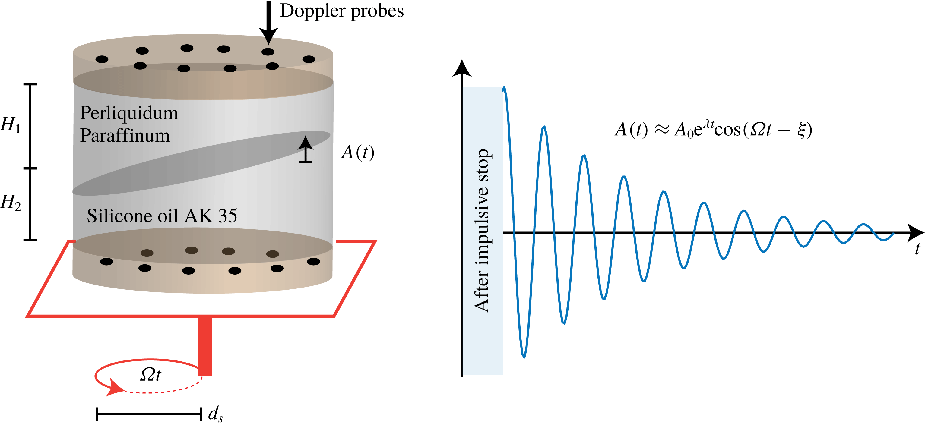
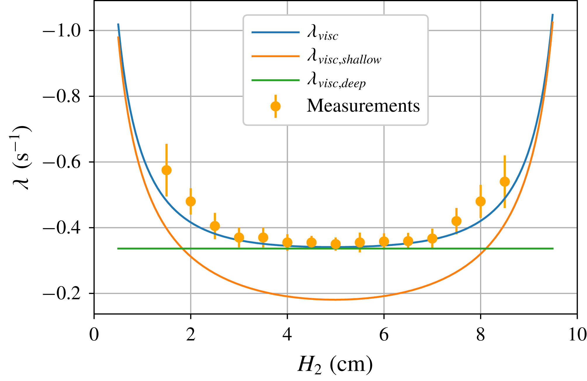
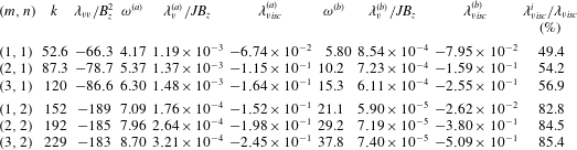
The article is structured as follows. In § 2, we present our linear stability model, formulated for idealized cylindrical cells and using the analytical tools of perturbation theory. The choice for cylindrical geometry is deliberately made to simplify the analysis as much as possible: rotating waves that are typically driven by metal pad roll instability exist in this geometry as simple exponential eigenmodes, not as superpositions of standing waves (the case in rectangular cells). The choice for a perturbative approach is motivated by the fact that, in a limited parameter range, all physical effects remain analytically tractable. This approach yields explicit formulas for growth rate, frequency shift and damping rate of different waveforms that are rarely available in existing metal roll theories. Note that we are not the first to propose the use of a perturbation method in metal pad roll theory: Descloux & Romerio (Reference Descloux and Romerio1989) already outlined this approach quite a while ago in rectangular cells, but explicit, readily applicable formulas were never derived. In § 3, we present the results of some purely hydrodynamic experiments that serve to test the theoretical viscous damping rates estimated by our theory. These experimental data points are by-products of a novel experimental study on orbital sloshing in two and three layer fluid systems (Horstmann, Wylega & Weier Reference Horstmann, Wylega and Weier2019). In § 4, we seek to validate the theoretical model numerically in the small laboratory-scale cylindrical reduction cell briefly discussed in Flueck et al. (Reference Flueck, Hofer, Picasso, Rappaz and Steiner2009) and Steiner (Reference Steiner2009). This allows for a precise and critical comparison with most aspects of the linear stability theory and, vice versa, serves as a critical benchmark to both our numerical solvers. In § 5, we apply our linear stability model to hypothetically large and shallow industrial-scale cells. In this section, we also provide a formula for the viscously controlled threshold
 $\unicode[STIX]{x1D6FD}_{c}$
of the metal pad roll instability in a cylindrical geometry. We also show that the proposed theory can quantitatively reproduce the numerically measured growth rates (Weber et al.
Reference Weber, Beckstein, Galindo, Herreman, Nore, Stefani and Weier2017a
) of the metal pad roll instability in cylindrical Mg–Sb liquid metal batteries. We then use our model to estimate the minimal radius
 $R_{c}$
below which no metal pad instability can occur in liquid metal batteries with strongly decoupled layers. In § 6, we conclude and discuss some perspectives of our study.
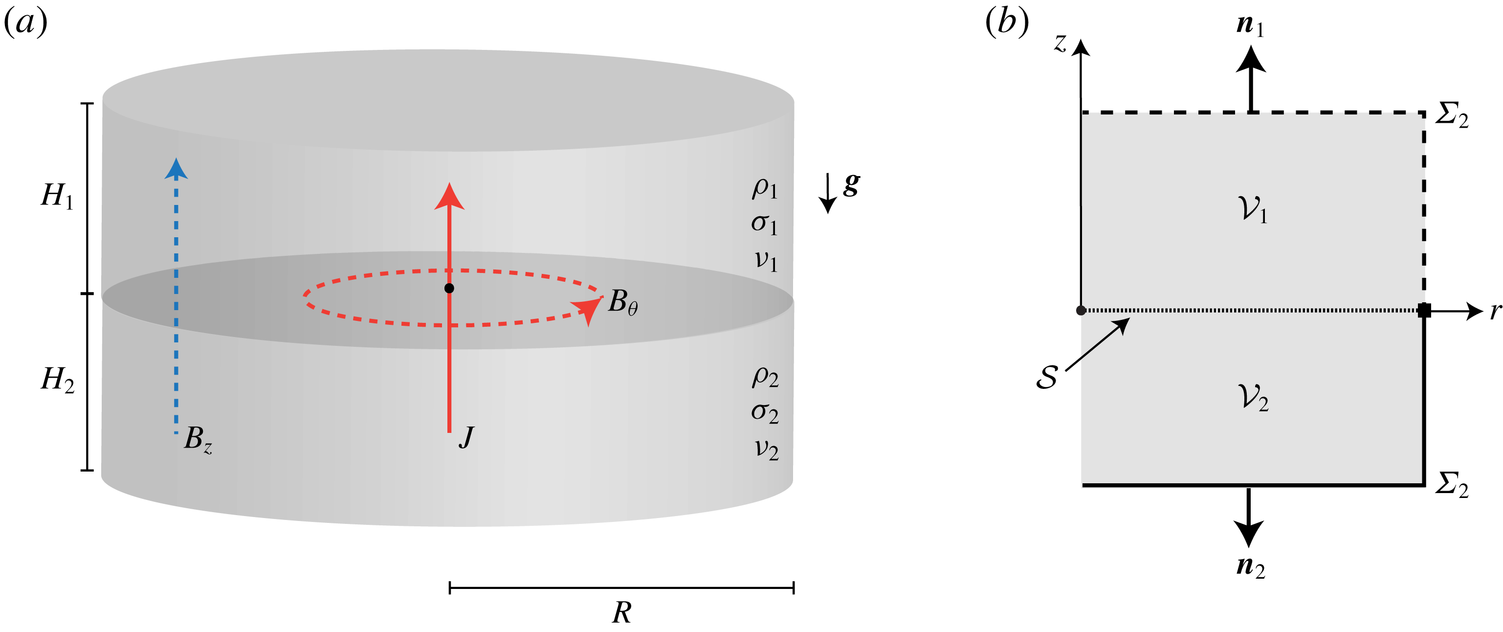
Sketch of cylindrical model cell and notation. (a) Two fluid layers with different densities
 $\unicode[STIX]{x1D70C}_{1},\unicode[STIX]{x1D70C}_{2}$
and respective heights
 $H_{1},H_{2}$
are stably superposed in a cylindrical container of radius
 $R$
due to gravity
 $\boldsymbol{g}$
. The layers have different electrical conductivities and kinematic viscosities denoted as
 $\unicode[STIX]{x1D70E}_{i},\unicode[STIX]{x1D708}_{i},i=1,2$
. A vertical electrical current
 $J\boldsymbol{e}_{z}$
runs through the cell (red full line) which generates an azimuthal magnetic field
 $B_{\unicode[STIX]{x1D703}}$
(red dashed line). We also suppose a homogenous and vertical background magnetic field
 $B_{z}$
(blue dashed line). (b) We use cylindrical coordinates
 $(r,\unicode[STIX]{x1D703},z)$
and denote
 $V_{i},i=1,2$
for both fluid regions.
 $\unicode[STIX]{x1D6F4}_{i},i=1,2$
refer to the rigid boundaries,
 ${\mathcal{S}}$
to the free interface at rest.
 $\boldsymbol{n}_{i}$
is the external normal on both fluid regions.

2 Linear stability theory
2.1 Equilibrium state and notation
The cylindrical cell under consideration in this paper is sketched in figure 1. We align the axis of symmetry with the
 $z$
-axis of a cylindrical coordinate system (
 $r,\unicode[STIX]{x1D703},z$
) with unit vectors (
 $\boldsymbol{e}_{r},\boldsymbol{e}_{\unicode[STIX]{x1D703}},\boldsymbol{e}_{z}$
). At equilibrium, the cryolite and aluminium layers (subscripts
 $i=1,2$
) occupy the volumes
 $$\begin{eqnarray}\left.\begin{array}{@{}c@{}}{\mathcal{V}}_{1}:(r,\unicode[STIX]{x1D703},z)\in [0,R]\times [0,2\unicode[STIX]{x03C0})\times [0,H_{1}],\\ {\mathcal{V}}_{2}:(r,\unicode[STIX]{x1D703},z)\in [0,R]\times [0,2\unicode[STIX]{x03C0})\times [-H_{2},0],\end{array}\right\}\end{eqnarray}$$
where
 $R$
is the radius of the cell and
 $H_{i}$
are the heights of the two layers. We denote
 $\unicode[STIX]{x1D6FF}V_{i}$
the boundary of each fluid domain and split each boundary
 $\unicode[STIX]{x1D6FF}{\mathcal{V}}_{i}$
as follows;
 $\unicode[STIX]{x1D6FF}{\mathcal{V}}_{i}=\unicode[STIX]{x1D6F4}_{i}\cup {\mathcal{S}}$
, with
 $\unicode[STIX]{x1D6F4}_{i}$
the rigid boundary and
 ${\mathcal{S}}$
the interface at rest. We denote as
 $\boldsymbol{n}_{i}$
the outward normal on
 $\unicode[STIX]{x1D6FF}{\mathcal{V}}_{i}.$
The electrical conductivity, density, kinematic viscosity of both fluids are denoted by
 $\unicode[STIX]{x1D70E}_{i},\unicode[STIX]{x1D70C}_{i},\unicode[STIX]{x1D708}_{i}$
, respectively. The surface tension of the interface between the two fluids is denoted by
 $\unicode[STIX]{x1D6FE}_{1|2}$
. We suppose that the interface touches the lateral wall with a contact angle of
 $90^{\circ }$
and that it slides freely.
If the cell is at equilibrium, both fluids are at rest. The fluids are subject to gravity
 $\boldsymbol{g}=-g\boldsymbol{e}_{z}$
. A homogenous electrical current density
 $\boldsymbol{J}=J\boldsymbol{e}_{z}$
runs through the cell (in reduction cells,
 $J<0$
always). This current generates an azimuthal magnetic field
 $B_{\unicode[STIX]{x1D703}}=\unicode[STIX]{x1D707}_{0}Jr/2$
and we suppose that a uniform external magnetic field
 $\boldsymbol{B}^{e}=B_{z}\boldsymbol{e}_{z}$
is present. Horizontal components of the external magnetic fields are not considered here because one can show that they have no impact on the instability, see appendix C. The total magnetic field is denoted
 $\boldsymbol{B}=B_{\unicode[STIX]{x1D703}}\boldsymbol{e}_{\unicode[STIX]{x1D703}}+B_{z}\boldsymbol{e}_{z}$
. The above state is a magnetohydrodynamic equilibrium configuration if the hydrodynamic pressure is
 $P_{i}=P_{\ast }-\unicode[STIX]{x1D70C}_{i}gz-\unicode[STIX]{x1D707}_{0}J^{2}r^{2}/4$
and the electrical potential is
 $\unicode[STIX]{x1D6F7}_{i}=\unicode[STIX]{x1D6F7}_{\ast }-Jz/\unicode[STIX]{x1D70E}_{i}$
with
 $P_{\ast },\unicode[STIX]{x1D6F7}_{\ast }$
arbitrary and constant offsets.
Although it appears as a detail, the hypothesis on the contact angle is in fact rather crucial to our stability theory. A more realistic contact angle, possibly different from
 $90^{\circ }$
, may result in a very different base state (such as figure 6 of Flueck et al. (Reference Flueck, Hofer, Picasso, Rappaz and Steiner2009)) with a deformed interface, inhomogeneous current density and possibly even capillary induced electro-vortex flows. The stability analysis of this kind of base state is evidently much more difficult, and this explains why we have limited our model to the simplified case of a freely sliding contact angle of
 $90^{\circ }$
. This configuration admits a simple base state with a flat interface, homogenous current and no flow. This implies that we only deal with some possible effects of capillarity but certainly not all.
2.2 The instability mechanism that we model
Illustration of a metal pad roll instability mechanism in an idealized cylindrical reduction cell. (a) Equilibrium cell with electrolysis current
 $\boldsymbol{J}$
and external vertical magnetic field
 $\boldsymbol{B}^{e}=B_{z}\boldsymbol{e}_{z}$
. (b) Snapshot of a small amplitude rotating wave with rotation speed
 $\unicode[STIX]{x1D714}$
and accompanying flow
 $\boldsymbol{u}$
in top and bottom layers. (c) Due to the wave, current density redistributes to preferentially pass through the shallower parts of the cryolite. (d) The current excess
 $\boldsymbol{j}$
is horizontal in the aluminium and interacts there with
 $\boldsymbol{B}^{e}$
to create a Lorentz force
 $\boldsymbol{j}\times \boldsymbol{B}^{e}$
that pushes in the direction of the flow
 $\boldsymbol{u}$
, amplifying the rotating wave as a result.

In figure 2, we illustrate the instability mechanism that is captured by our model. Overall, it is very similar to Sele’s mechanism (Sele Reference Sele1977), but the cylindrical geometry allows an essential, simplifying difference in presentation. Rather than finding the amplification as a consequence of a coupling between transverse standing waves, we can, in a cylindrical geometry, more simply show that rotating waves amplify themselves.
Let us start with figure 2(a), that shows the equilibrium configuration: cryolite in the top layer, aluminium in the bottom layer and the reduction current flowing from top to bottom (
 $J<0$
). We choose the external vertical magnetic field
 $\boldsymbol{B}^{e}$
to be upward. In (b), we perturb this equilibrium with a small rotating wave, rotating clockwise when seen from above, as suggested by the figure. Along with this wave comes the instantaneous fluid flow
 $\boldsymbol{u}$
, pointing as sketched, either towards (top) or away from (bottom) the observer. Through time, this entire pattern will rotate, and, in the absence of electromagnetic forces, slowly decay in magnitude because of viscous dissipation. In (c,d), we explain how the Lorentz force associated with this wave necessarily amplifies this wave. Since cryolite is a much worse conductor than aluminium, the current density
 $\boldsymbol{J}$
will deviate due to a current excess
 $\boldsymbol{j}$
, in order to preferentially pass through the shallower part of the cryolite. This is suggested by the thin and thick arrows of (c). (d) Shows how the current excess
 $\boldsymbol{j}$
typically loops in reduction cells, being mainly horizontal in the aluminium and mainly vertical in the cryolite. In the aluminium layer, this horizontal
 $\boldsymbol{j}$
interacts with the external vertical field
 $\boldsymbol{B}^{e}$
to create a Lorentz force
 $\boldsymbol{j}\times \boldsymbol{B}^{e}$
which pushes exactly in the direction of the instantaneous flow
 $\boldsymbol{u}$
. Precisely the same picture can be made at any rotated interface position and this means that positive power is permanently being injected into the rotating wave by the Lorentz force:
 $\boldsymbol{u}\boldsymbol{\cdot }(\boldsymbol{j}\times \boldsymbol{B}^{e})>0$
. Initially small rotating waves can therefore be electromagnetically amplified. Notice that the direction of rotation of the wave is a crucial element in the destabilization process: inverting
 $\unicode[STIX]{x1D714}$
, inverts the flow
 $\boldsymbol{u}$
and with
 $\boldsymbol{u}\boldsymbol{\cdot }(\boldsymbol{j}\times \boldsymbol{B}^{e})<0$
, the wave rotating in the opposite sense will be damped rather than magnified. Only waves rotating in one direction will be amplified and this direction obviously depends on the sign of
 $JB_{z}$
. In our theory, this amplification is captured in the growth rate denoted
 $\unicode[STIX]{x1D706}_{\mathit{v}}$
.
With the same kind of physical reasoning, one can understand why the azimuthal magnetic field,
 $B_{\unicode[STIX]{x1D703}}\boldsymbol{e}_{\unicode[STIX]{x1D703}}$
, cannot amplify rotating waves (nor standing waves). The Lorentz force
 $\boldsymbol{j}\times (B_{\unicode[STIX]{x1D703}}\boldsymbol{e}_{\unicode[STIX]{x1D703}})$
is radial in the cryolite and vertical in the aluminium layer, i.e. always perpendicular to the instantaneous flow
 $\boldsymbol{u}$
. The azimuthal field can therefore not cause an amplification nor a damping. In our theory we find that the azimuthal field causes a shift in the frequency of the wave (denoted by
 $\unicode[STIX]{x1D6FF}_{\mathit{h}}$
), in agreement with the theoretical predictions of Sneyd (Reference Sneyd1985) and Sneyd & Wang (Reference Sneyd and Wang1994).
2.3 Linearized problem in the quasi-static limit
Now that we know how the equilibrium state can become unstable, we want to perform the linear stability analysis that takes into account viscous dissipation, magnetic dissipation and surface tension, and without making the shallow layer approximation. We start by linearizing the governing equations about the equilibrium state. Denoting
 $B=\max (\unicode[STIX]{x1D707}_{0}JR,B_{z})$
the typical scale for the magnetic field strength, we suppose that the Lundquist numbers
 $Lu_{i}$
in both layers
 $i=1,2$
remain very low,
 $$\begin{eqnarray}Lu_{i}=\unicode[STIX]{x1D70E}_{i}\unicode[STIX]{x1D707}_{0}BR/\sqrt{\unicode[STIX]{x1D70C}_{i}\unicode[STIX]{x1D707}_{0}}\ll 1.\end{eqnarray}$$
This hypothesis allows us to use the quasi-static approximation of MHD, in which the electrical field derives from the electrical potential. Denoting by
 $(\boldsymbol{u}_{i},p_{i},\boldsymbol{b}_{i},\boldsymbol{j}_{i},\unicode[STIX]{x1D711}_{i})$
perturbations for the velocity, the pressure, the magnetic induction, the current density and the electrical potential, we find the linearized perturbation equations of the magnetohydrodynamic stability problem to be
 $$\begin{eqnarray}\displaystyle \unicode[STIX]{x1D70C}_{i}\unicode[STIX]{x2202}_{t}\boldsymbol{u}_{i}+\unicode[STIX]{x1D735}p_{i} & = & \displaystyle \boldsymbol{J}\times \boldsymbol{b}_{i}+\boldsymbol{j}_{i}\times \boldsymbol{B}+\unicode[STIX]{x1D70C}_{i}\unicode[STIX]{x1D708}_{i}\unicode[STIX]{x1D6FB}^{2}\boldsymbol{u}_{i},\end{eqnarray}$$
 $$\begin{eqnarray}\displaystyle \unicode[STIX]{x1D735}\boldsymbol{\cdot }\boldsymbol{u}_{i} & = & \displaystyle 0,\end{eqnarray}$$
 $$\begin{eqnarray}\displaystyle \boldsymbol{j}_{i} & = & \displaystyle \unicode[STIX]{x1D70E}_{i}(-\unicode[STIX]{x1D735}\unicode[STIX]{x1D711}_{i}+\boldsymbol{u}_{i}\times \boldsymbol{B}),\quad \unicode[STIX]{x1D735}\boldsymbol{\cdot }\boldsymbol{j}_{i}=0,\end{eqnarray}$$
 $$\begin{eqnarray}\displaystyle \unicode[STIX]{x1D735}\times \boldsymbol{b}_{i} & = & \displaystyle \unicode[STIX]{x1D707}_{0}\boldsymbol{j}_{i},\quad \unicode[STIX]{x1D735}\boldsymbol{\cdot }\boldsymbol{b}_{i}=0.\end{eqnarray}$$
 $\unicode[STIX]{x1D6F4}_{i}$
is that of impermeability
 $$\begin{eqnarray}\boldsymbol{u}_{i}\boldsymbol{\cdot }\boldsymbol{n}_{i}=0|_{\unicode[STIX]{x1D6F4}_{i}},\end{eqnarray}$$
to which we must add
 $\boldsymbol{u}_{\boldsymbol{i}}\times \boldsymbol{n}_{i}=0|_{\unicode[STIX]{x1D6F4}_{i}}$
when the viscous effects are accounted for. On the interface
 ${\mathcal{S}}$
, which we locate at
 $z=\unicode[STIX]{x1D702}(r,\unicode[STIX]{x1D703},t)$
, the essential inviscid boundary conditions are
 $$\begin{eqnarray}\displaystyle \unicode[STIX]{x2202}_{t}\unicode[STIX]{x1D702} & = & \displaystyle u_{1,z}|_{z=0},\end{eqnarray}$$
 $$\begin{eqnarray}\displaystyle \unicode[STIX]{x2202}_{t}\unicode[STIX]{x1D702} & = & \displaystyle u_{2,z}|_{z=0},\end{eqnarray}$$
 $$\begin{eqnarray}\displaystyle -\unicode[STIX]{x1D6FE}_{1|2}\unicode[STIX]{x1D6FB}^{2}\unicode[STIX]{x1D702}+(\unicode[STIX]{x1D70C}_{2}-\unicode[STIX]{x1D70C}_{1})g\unicode[STIX]{x1D702} & = & \displaystyle p_{2}|_{z=0}-p_{1}|_{z=0}.\end{eqnarray}$$
 $\unicode[STIX]{x1D6F4}_{i}$
, we suppose
 $$\begin{eqnarray}\displaystyle j_{1,r}|_{r=R} & = & \displaystyle 0,\end{eqnarray}$$
 $$\begin{eqnarray}\displaystyle j_{2,r}|_{r=R} & = & \displaystyle 0,\end{eqnarray}$$
 $$\begin{eqnarray}\displaystyle \unicode[STIX]{x1D711}_{1}|_{z=H_{1}} & = & \displaystyle 0,\end{eqnarray}$$
 $$\begin{eqnarray}\displaystyle j_{2,z}|_{z=-H_{2}} & = & \displaystyle 0.\end{eqnarray}$$
 ${\mathcal{S}}$
, the total normal current density (
 $\boldsymbol{n}\boldsymbol{\cdot }(\boldsymbol{J}+\boldsymbol{j}_{i})$
) and total electrical potential (
 $\unicode[STIX]{x1D6F7}_{i}+\unicode[STIX]{x1D711}_{i}$
) are continuous. Taylor expanding these conditions around
 $z=0$
, we find the linearized version of the continuity conditions as
 $$\begin{eqnarray}\displaystyle 0 & = & \displaystyle j_{1,z}|_{z=0}-j_{2,z}|_{z=0},\end{eqnarray}$$
 $$\begin{eqnarray}\displaystyle J(\unicode[STIX]{x1D70E}_{2}^{-1}-\unicode[STIX]{x1D70E}_{1}^{-1})\unicode[STIX]{x1D702} & = & \displaystyle \unicode[STIX]{x1D711}_{2}|_{z=0}-\unicode[STIX]{x1D711}_{1}|_{z=0}.\end{eqnarray}$$
 $\unicode[STIX]{x1D711}_{i}$
(and so currents
 $\boldsymbol{j}_{i}$
) relate to the motion of the interface. Without a significant jump in conductivity, there is no potential difference directly caused by interface motions and no metal pad roll instability, as we will see.
Finally, for the magnetic induction driven by the electrical currents, we suppose the following boundary condition on the cylindrical boundary:
 $$\begin{eqnarray}\boldsymbol{e}_{r}\times \boldsymbol{b}_{i}|_{r=R}=0.\end{eqnarray}$$
Magnetic field behaviour at other boundaries is not specified, because it has no influence in the theoretical model that we develop. This boundary condition is obviously artificial but it avoids us having to explicitly calculate the magnetic field perturbation, which is never an easy task. The magnetic field perturbation
 $\boldsymbol{b}_{i}$
is anyway of secondary importance: it only appears through the term
 $\boldsymbol{J}\times \boldsymbol{b}_{i}$
that is not destabilizing according to our model. Many previous metal pad roll theories have directly ignored this term and according to Sun et al. (Reference Sun, Zikanov and Ziegler2004), this seems justified.
The linearized problem is now completely defined and so we can look for linear eigenmodes. Due to the stationarity of the equilibrium state, we look for fundamental solutions with a simple exponential time dependence. More precisely, if
 $f$
represents any of the relevant fields or components, we propose the ansatz
 $$\begin{eqnarray}f=\hat{f}\text{e}^{st},\end{eqnarray}$$
and try to find the admissible (complex) eigenfunctions
 $\hat{f}$
and (complex) eigenvalues
 $s\in \mathbb{C}$
. We call
 $\text{Re}(s)$
the growth rate and
 $\text{Im}(s)$
the frequency. If
 $\text{Re}(s)>0$
, the eigenmode is linearly unstable and if
 $\text{Im}(s)\neq 0$
the solution is wave like. Using a numerical approach it is possible to solve this linear eigenvalue problem. In the following sections we rather use a perturbative approach to find a suitable approximation to
 $s$
, valid in some parameter range.
2.4 Free inviscid gravito-capillary waves
Our perturbative approach is based on the free inviscid gravito-capillary waves that form a family of eigensolutions in the absence of an electrolysis current (
 $J=0$
), vertical magnetic field (
 $B_{z}=0$
) and without viscosity (
 $\unicode[STIX]{x1D708}=0$
). In that case, the following hydrodynamic field
 $$\begin{eqnarray}[\boldsymbol{u}_{i},p_{i},\unicode[STIX]{x1D702}]=[\widehat{\boldsymbol{u}}_{i},\widehat{p}_{i},\widehat{\unicode[STIX]{x1D702}}]\text{e}^{\text{i}\unicode[STIX]{x1D714}t},\end{eqnarray}$$
is a solution to the linearized problem defined above. The hydrodynamic fields
 $\widehat{\boldsymbol{u}}_{i},\widehat{p}_{i},\widehat{\unicode[STIX]{x1D702}}$
correspond to the classical potential wave solution (see Lamb Reference Lamb1945),
 $$\begin{eqnarray}\left[\begin{array}{@{}c@{}}\widehat{\boldsymbol{u}}_{i}\\ \widehat{p}_{i}\\ \widehat{\unicode[STIX]{x1D702}}\end{array}\right]=\left[\begin{array}{@{}c@{}}\unicode[STIX]{x1D735}\widehat{\unicode[STIX]{x1D719}}_{i}\\ -\unicode[STIX]{x1D70C}_{i}(\text{i}\unicode[STIX]{x1D714})\widehat{\unicode[STIX]{x1D719}}_{i}\\ \unicode[STIX]{x2202}_{z}\widehat{\unicode[STIX]{x1D719}}_{i}/(\text{i}\unicode[STIX]{x1D714})\end{array}\right],\end{eqnarray}$$
with
 $$\begin{eqnarray}\left[\begin{array}{@{}c@{}}\widehat{\unicode[STIX]{x1D719}}_{1}\\ \widehat{\unicode[STIX]{x1D719}}_{2}\\ \widehat{\unicode[STIX]{x1D702}}\end{array}\right]=A\,R\left[\begin{array}{@{}r@{}}(\unicode[STIX]{x1D714}/k)\cosh (k(z-H_{1}))/\sinh (kH_{1})\\ -(\unicode[STIX]{x1D714}/k)\cosh (k(z+H_{2}))/\sinh (kH_{2})\\ \text{i}\end{array}\right]\text{J}_{m}(kr)\text{e}^{\text{i}m\unicode[STIX]{x1D703}}.\end{eqnarray}$$
The non-dimensional amplitude
 $A$
is arbitrary here. The functions
 $\text{J}_{m}$
are Bessel functions,
 $m\in \mathbb{Z}$
is the azimuthal wavenumber and
 $k$
is a radial wavenumber that takes the discrete values
 $$\begin{eqnarray}k=\unicode[STIX]{x1D705}_{mn}/R,\quad \text{J}_{m}^{\prime }(\unicode[STIX]{x1D705}_{mn})=0,\end{eqnarray}$$
to ensure that the boundary condition
 $u_{r}|_{r=R}=0$
is satisfied. We note by
 $\unicode[STIX]{x1D705}_{mn}$
the
 $n$
th zero of the derivative of the Bessel function
 $\text{J}_{m}$
(
 $\unicode[STIX]{x1D705}_{11}\approx 1.84$
,
 $\unicode[STIX]{x1D705}_{21}\approx 3.05$
,
 $\unicode[STIX]{x1D705}_{31}\approx 4.20$
). The natural frequency
 $\unicode[STIX]{x1D714}$
of the (free) waves is
 $$\begin{eqnarray}\unicode[STIX]{x1D714}=\pm \sqrt{\frac{(\unicode[STIX]{x1D70C}_{2}-\unicode[STIX]{x1D70C}_{1})gk+\unicode[STIX]{x1D6FE}_{1|2}k^{3}}{{\displaystyle \frac{\unicode[STIX]{x1D70C}_{2}}{\tanh (kH_{2})}}+{\displaystyle \frac{\unicode[STIX]{x1D70C}_{1}}{\tanh (kH_{1})}}}},\end{eqnarray}$$
and may be either positive or negative for a fixed
 $m$
. The solution presented here (see (2.10)) has a simple harmonic form, but the real flow is always real valued. Taking the real part of (2.10), one finds rotating waves with positive rotation speed if
 $m\unicode[STIX]{x1D714}<0$
(anti-clockwise when seen from above) and negative rotation speed if
 $m\unicode[STIX]{x1D714}>0$
(clockwise when seen from above). Two oppositely rotating waves can also be superposed to give standing waves.
2.5 Sufficient conditions to apply perturbation methods
Perturbation methods may only be used when the Lorentz force and the viscous forces appear as small perturbations in the momentum balance. Symbolically, this means that
 $$\begin{eqnarray}[\boldsymbol{J}\times \boldsymbol{b}_{i}],[\boldsymbol{j}_{i}\times \boldsymbol{B}],[\unicode[STIX]{x1D70C}_{i}\unicode[STIX]{x1D708}_{i}\unicode[STIX]{x1D6FB}^{2}\boldsymbol{u}_{i}]\ll [\unicode[STIX]{x1D70C}_{i}\unicode[STIX]{x2202}_{t}\boldsymbol{u}_{i}],[\unicode[STIX]{x1D735}p_{i}],\end{eqnarray}$$
in terms of orders of magnitude (denoted using square brackets). This limits the parameter space that can be explored and we want to estimate these limits here.
For simplicity, we assume
 $J,B,\unicode[STIX]{x1D714}\geqslant 0$
to avoid the use of absolute values. We use
 $[\boldsymbol{x}]=R$
as the space scale rather than
 $k^{-1}$
since this is more explicit (and anyway similar to
 $k^{-1}$
for long-wavelength waves). We denote
 $[\boldsymbol{u}_{i}]=U$
the velocity scale, which is arbitrary in this linear approach. For hydrodynamic waves, we can estimate
 $$\begin{eqnarray}[\unicode[STIX]{x1D70C}_{i}\unicode[STIX]{x2202}_{t}\boldsymbol{u}_{i}]\sim \unicode[STIX]{x1D70C}_{i}\unicode[STIX]{x1D714}U,\quad [p_{i}]\sim \unicode[STIX]{x1D70C}_{i}\unicode[STIX]{x1D714}RU.\end{eqnarray}$$
The viscous term has the following order of magnitude:
 $$\begin{eqnarray}[\unicode[STIX]{x1D70C}_{i}\unicode[STIX]{x1D708}_{i}\unicode[STIX]{x1D6FB}^{2}\boldsymbol{u}_{i}]\sim \unicode[STIX]{x1D70C}_{i}\unicode[STIX]{x1D708}_{i}U/R^{2}.\end{eqnarray}$$
We introduce
 $B$
as the order of magnitude of the imposed magnetic field
 $$\begin{eqnarray}[\boldsymbol{B}]\sim B=\left\{\begin{array}{@{}rcl@{}}\unicode[STIX]{x1D707}_{0}JR & \longrightarrow & \text{azimuthal},\\ B_{z} & \longrightarrow & \text{vertical}.\end{array}\right.\end{eqnarray}$$
We can use two independent estimates related to either the azimuthal or to the vertical magnetic field. From Ohm’s law (2.3c ), we then estimate the magnitude of the induction term as
 $$\begin{eqnarray}[\unicode[STIX]{x1D70E}_{i}\boldsymbol{u}_{i}\times \boldsymbol{B}]\sim \unicode[STIX]{x1D70E}_{i}UB.\end{eqnarray}$$
Still in Ohm’s law (2.3c
), the electrical potential term may have the same order of magnitude as
 $\boldsymbol{u}_{i}\times \boldsymbol{B}$
, but the interface deformations caused by the waves can also lead to a different magnitude which can be estimated from the boundary conditions (2.5a
), (2.5b
) and (2.7b
). This yields the following two different estimates
 $$\begin{eqnarray}[-\unicode[STIX]{x1D70E}_{i}\unicode[STIX]{x1D735}\unicode[STIX]{x1D711}_{i}]\sim \left\{\begin{array}{@{}rcl@{}}JU/(\unicode[STIX]{x1D714}R) & \longrightarrow & \text{interface deformations},\\ \unicode[STIX]{x1D70E}_{i}UB & \longrightarrow & \text{induction by the flow}.\end{array}\right.\end{eqnarray}$$
Using Ampère’s law (2.3d ), we can calculate the associated magnetic field perturbation magnitudes
 $$\begin{eqnarray}[\boldsymbol{b}_{i}]\sim \left\{\begin{array}{@{}l@{}}\unicode[STIX]{x1D707}_{0}JU/\unicode[STIX]{x1D714},\\ \unicode[STIX]{x1D707}_{0}\unicode[STIX]{x1D70E}_{i}URB.\end{array}\right.\end{eqnarray}$$
All the orders of magnitude of the different fields have been estimated so we can now reformulate the inequalities (2.15). The trivial but sufficient condition to model viscous effects perturbatively is
 $$\begin{eqnarray}[\unicode[STIX]{x1D70C}_{i}\unicode[STIX]{x1D708}_{i}\unicode[STIX]{x1D6FB}^{2}u_{i}]\ll [\unicode[STIX]{x1D70C}_{i}\unicode[STIX]{x2202}_{t}\boldsymbol{u}_{i}]\quad \Leftrightarrow \quad Re_{i}=\frac{\unicode[STIX]{x1D714}R^{2}}{\unicode[STIX]{x1D708}_{i}}\gg 1,\end{eqnarray}$$
which we recognize as a constraint on Reynolds numbers based on the properties of the wave. A set of sufficient conditions that allows us to model the effects of the Lorentz force using perturbation methods is then
 $$\begin{eqnarray}\displaystyle [\boldsymbol{J}\times \boldsymbol{b}_{i}]\ll [\unicode[STIX]{x1D70C}_{i}\unicode[STIX]{x2202}_{t}\boldsymbol{u}_{i}] & \quad \Leftrightarrow \quad & \displaystyle \left\{\begin{array}{@{}l@{}}{\displaystyle \frac{\unicode[STIX]{x1D707}_{0}J^{2}}{\unicode[STIX]{x1D70C}_{i}\unicode[STIX]{x1D714}^{2}}}\ll 1,\\ {\displaystyle \frac{\unicode[STIX]{x1D707}_{0}\unicode[STIX]{x1D70E}_{i}JRB}{\unicode[STIX]{x1D70C}_{i}\unicode[STIX]{x1D714}}}\ll 1,\end{array}\right.\end{eqnarray}$$
 $$\begin{eqnarray}\displaystyle [\boldsymbol{j}_{i}\times \boldsymbol{B}]\ll [\unicode[STIX]{x1D70C}_{i}\unicode[STIX]{x2202}_{t}\boldsymbol{u}_{i}] & \quad \Leftrightarrow \quad & \displaystyle \left\{\begin{array}{@{}l@{}}{\displaystyle \frac{JB}{\unicode[STIX]{x1D70C}_{i}\unicode[STIX]{x1D714}^{2}R}}\ll 1,\\ {\displaystyle \frac{\unicode[STIX]{x1D70E}_{i}B^{2}}{\unicode[STIX]{x1D70C}_{i}\unicode[STIX]{x1D714}}}\ll 1.\end{array}\right.\end{eqnarray}$$
2.6 Perturbative calculation of growth rates and frequency shifts
In this technical section, we calculate the theoretical expression for the complex eigenvalue
 $s$
that characterizes the exponential behaviour (
 ${\sim}\text{exp}(st)$
) of the linear eigenmode. Since the perturbation methods that we are going to use are rather involved, we first give a brief overview of the methodology. The theoretical expression for
 $s$
will be split as
 $$\begin{eqnarray}s=\text{i}\unicode[STIX]{x1D714}+\underbrace{(\unicode[STIX]{x1D706}+\text{i}\unicode[STIX]{x1D6FF})}_{\unicode[STIX]{x1D6FC}}.\end{eqnarray}$$
Here
 $\unicode[STIX]{x1D714}$
is the inviscid gravity wave frequency and
 $\unicode[STIX]{x1D6FC}$
is a small complex shift induced by the Lorentz and the viscous forces. We define
 $\unicode[STIX]{x1D706}=\text{Re}(\unicode[STIX]{x1D6FC})$
, the growth rate of the gravity wave, and
 $\unicode[STIX]{x1D6FF}=\text{Im}(\unicode[STIX]{x1D6FC})$
, the frequency shift. The growth rate is decomposed into several independent terms as follows:
 $$\begin{eqnarray}\unicode[STIX]{x1D706}=\underbrace{\unicode[STIX]{x1D706}_{\mathit{v}}}_{destab.}+\underbrace{\unicode[STIX]{x1D706}_{\mathit{vv}}+\unicode[STIX]{x1D706}_{\mathit{hh}}}_{quasi\text{-}static}+\underbrace{\unicode[STIX]{x1D706}_{\mathit{visc}}}_{visc.damping}.\end{eqnarray}$$
The first term
 $\unicode[STIX]{x1D706}_{\mathit{v}}\lessgtr 0$
is the potentially destabilizing term and directly relates to the instability mechanism sketched in figure 2, where the external vertical magnetic field
 $B_{z}$
(hence the suffix
 $~_{\mathit{v}}$
) plays an important role in destabilizing a rotating wave. The terms
 $\unicode[STIX]{x1D706}_{\mathit{vv}},\unicode[STIX]{x1D706}_{\mathit{hh}}$
are negative in general. These corrections are quadratic in the vertical and horizontal magnetic field magnitudes (hence the suffixes
 $~_{\mathit{vv}}$
and
 $~_{\mathit{hh}}$
) and are often ignored in metal pad roll theory. They relate to the inductive terms
 $\unicode[STIX]{x1D70E}_{i}\boldsymbol{u}_{i}\times \boldsymbol{B}$
that exist in the quasi-static version of Ohm’s law and that in general cause a magnetic damping. The term
 $\unicode[STIX]{x1D706}_{\mathit{visc}}<0$
captures the viscous damping of the gravity waves. We similarly decompose the frequency shift as follows:
 $$\begin{eqnarray}\unicode[STIX]{x1D6FF}=\unicode[STIX]{x1D6FF}_{\mathit{h}}+\unicode[STIX]{x1D6FF}_{\mathit{vh}}+\unicode[STIX]{x1D6FF}_{\mathit{visc}}.\end{eqnarray}$$
The term
 $\unicode[STIX]{x1D6FF}_{\mathit{h}}$
is the result of the Lorentz force interaction of
 $\boldsymbol{j}_{i}$
, caused by the interface deformation, with the background horizontal (azimuthal) magnetic field
 $B_{\unicode[STIX]{x1D703}}=\unicode[STIX]{x1D707}_{0}Jr/2$
(hence the suffix
 $~_{\mathit{h}}$
). The term
 $\unicode[STIX]{x1D6FF}_{\mathit{vh}}$
is a small quasi-static correction related to both
 $B_{\unicode[STIX]{x1D703}}$
and
 $B_{z}$
, and
 $\unicode[STIX]{x1D6FF}_{\mathit{visc}}$
is a frequency shift caused by viscous effects.
Above, we have provided sufficient conditions to apply a perturbation method. Necessary conditions can be derived a posteriori by verifying that
 $$\begin{eqnarray}\left|\frac{\unicode[STIX]{x1D706}_{\mathit{v}}}{\unicode[STIX]{x1D714}}\right|,\quad \left|\frac{\unicode[STIX]{x1D706}_{\mathit{vv}}}{\unicode[STIX]{x1D714}}\right|,\quad \left|\frac{\unicode[STIX]{x1D706}_{\mathit{hh}}}{\unicode[STIX]{x1D714}}\right|,\quad \left|\frac{\unicode[STIX]{x1D706}_{\mathit{visc}}}{\unicode[STIX]{x1D714}}\right|,\quad \left|\frac{\unicode[STIX]{x1D6FF}_{\mathit{h}}}{\unicode[STIX]{x1D714}}\right|,\quad \left|\frac{\unicode[STIX]{x1D6FF}_{\mathit{vh}}}{\unicode[STIX]{x1D714}}\right|,\quad \left|\frac{\unicode[STIX]{x1D6FF}_{\mathit{visc}}}{\unicode[STIX]{x1D714}}\right|\ll 1.\end{eqnarray}$$
When these conditions are not met, the theoretical formulas we deduce in the following sections may not be accurate or may even be wrong. This observation must be kept in mind.
2.6.1 Metal pad roll instability in the magneto-static and inviscid limit:
 $\unicode[STIX]{x1D706}_{\mathit{v}}$
and
$\unicode[STIX]{x1D6FF}_{\mathit{h}}$


In this section, we focus on the leading terms in the growth rate and frequency shift formulas,
 $\unicode[STIX]{x1D706}_{\mathit{v}}$
and
 $\unicode[STIX]{x1D6FF}_{\mathit{h}}$
. This can be done in the inviscid limit
 $\unicode[STIX]{x1D708}_{i}=0$
, and, assuming that the magnetostatic approximation of Ohm’s law
 $$\begin{eqnarray}\boldsymbol{j}_{i}\approx -\unicode[STIX]{x1D70E}_{i}\unicode[STIX]{x1D735}\unicode[STIX]{x1D711}_{i}\end{eqnarray}$$
can be used. This a common supplementary assumption in most metal pad roll theory. Using
 $[\unicode[STIX]{x1D70E}_{i}\unicode[STIX]{x1D735}\unicode[STIX]{x1D711}_{i}]=JU/(\unicode[STIX]{x1D714}R)$
and
 $[\unicode[STIX]{x1D70E}_{i}\boldsymbol{u}_{i}\times \boldsymbol{B}]=\unicode[STIX]{x1D70E}_{i}UB$
, from our order of magnitude analysis we find a sufficient condition
 $$\begin{eqnarray}[\unicode[STIX]{x1D70E}_{i}\boldsymbol{u}_{i}\times \boldsymbol{B}]\ll [-\unicode[STIX]{x1D70E}_{i}\unicode[STIX]{x1D735}\unicode[STIX]{x1D711}_{i}]\quad \Leftrightarrow \quad \unicode[STIX]{x1D70E}_{i}\unicode[STIX]{x1D714}RB/J\ll 1,\end{eqnarray}$$
which we suppose valid in this first section. As a result of the inviscid and magneto-static hypothesis, both viscous and Joule dissipation will be absent in this entire section.
We propose the following ansatz to the inviscid and magneto-static limit of the linearized problem defined in § 2.3:
 $$\begin{eqnarray}[\boldsymbol{u}_{i},p_{i},\unicode[STIX]{x1D702},\boldsymbol{j}_{i},\unicode[STIX]{x1D711}_{i},\boldsymbol{b}_{i}]=\left(\left[\widehat{\boldsymbol{u}}_{i},\widehat{p}_{i},\widehat{\unicode[STIX]{x1D702}},\widehat{\boldsymbol{j}}_{i},\widehat{\unicode[STIX]{x1D711}}_{i},\widehat{\boldsymbol{b}}_{i}\right]+\left[\widetilde{\boldsymbol{u}}_{i},\widetilde{p}_{i},\widetilde{\unicode[STIX]{x1D702}},\widetilde{\boldsymbol{j}}_{i},\widetilde{\unicode[STIX]{x1D711}}_{i},\widetilde{\boldsymbol{b}}_{i}\right]\right)\text{e}^{\text{i}\unicode[STIX]{x1D714}t}\text{e}^{\unicode[STIX]{x1D6FC}t}.\end{eqnarray}$$
In this notation, the tilded variables are small perturbations with respect to the hatted variables, and the complex shift
 $\unicode[STIX]{x1D6FC}$
is small with respect to
 $\unicode[STIX]{x1D714}$
. Here
 $\unicode[STIX]{x1D714}$
is the frequency of the gravity waves. We inject this ansatz into the governing equations and we treat the Lorentz force term perturbatively. At leading order, we find the following balance equations:
 $$\begin{eqnarray}\left.\begin{array}{@{}c@{}}\unicode[STIX]{x1D70C}_{i}(i\unicode[STIX]{x1D714})\widehat{\boldsymbol{u}}_{i}+\unicode[STIX]{x1D735}\widehat{p}_{i}=0,\quad \unicode[STIX]{x1D735}\boldsymbol{\cdot }\widehat{\boldsymbol{u}}_{i}=0,\\ \widehat{\boldsymbol{j}}_{i}=-\unicode[STIX]{x1D70E}_{i}\unicode[STIX]{x1D735}\widehat{\unicode[STIX]{x1D711}}_{i},\quad \unicode[STIX]{x1D735}\boldsymbol{\cdot }\widehat{\boldsymbol{j}}_{i}=0,\\ \unicode[STIX]{x1D735}\times \widehat{\boldsymbol{b}}_{i}=\unicode[STIX]{x1D707}_{0}\widehat{\boldsymbol{j}}_{i},\quad \unicode[STIX]{x1D735}\boldsymbol{\cdot }\widehat{\boldsymbol{b}}_{i}=0.\end{array}\right\}\end{eqnarray}$$
Notice that the Lorentz force is absent in the momentum equation. The boundary conditions for the hatted fields can be copied from ((2.4)
 $\rightarrow$
(2.8)) after replacing
 $\unicode[STIX]{x2202}_{t}\rightarrow \text{i}\unicode[STIX]{x1D714}$
. We have to solve this problem in order to specify all the first-order quantities. The hydrodynamic fields
 $\widehat{\boldsymbol{u}}_{i},\widehat{p}_{i},\widehat{\unicode[STIX]{x1D702}}$
and the frequency
 $\unicode[STIX]{x1D714}$
have already been given above. The electrical potential
 $\widehat{\unicode[STIX]{x1D711}}_{i}$
is harmonic (
 $\unicode[STIX]{x1D6FB}^{2}\widehat{\unicode[STIX]{x1D711}}_{i}=0$
) and is related to the surface elevation
 $\widehat{\unicode[STIX]{x1D702}}$
by the jump condition (2.7b
). After some computations we find that
 $$\begin{eqnarray}\displaystyle \left[\begin{array}{@{}c@{}}\widehat{\unicode[STIX]{x1D711}}_{1}\\ \widehat{\unicode[STIX]{x1D711}}_{2}\end{array}\right] & = & \displaystyle JRA\frac{\unicode[STIX]{x1D70E}_{1}^{-1}-\unicode[STIX]{x1D70E}_{2}^{-1}}{\unicode[STIX]{x1D70E}_{1}^{-1}\tanh (kH_{1})+(\unicode[STIX]{x1D70E}_{2}\tanh (kH_{2}))^{-1}}\nonumber\\ \displaystyle & & \displaystyle \times \left[\begin{array}{@{}c@{}}-\text{i}\,\sinh (k(z-H_{1}))/(\unicode[STIX]{x1D70E}_{1}\cosh (kH_{1}))\\ -\text{i}\,\cosh (k(z+H_{2}))/(\unicode[STIX]{x1D70E}_{2}\sinh (kH_{2}))\end{array}\right]\text{J}_{m}(kr)\text{e}^{\text{i}m\unicode[STIX]{x1D703}}.\end{eqnarray}$$
The insulating side wall condition is automatically satisfied since
 $\text{J}_{m}^{\prime }(kR)=0$
by definition (see (2.13)). The electrical top and bottom boundary conditions are satisfied as well. The electrical currents,
 $\widehat{\boldsymbol{j}}_{i}=-\unicode[STIX]{x1D70E}_{i}\unicode[STIX]{x1D735}\unicode[STIX]{x1D711}_{i}$
are easily deduced from the potentials. The magnetic field perturbations
 $\widehat{\boldsymbol{b}}_{i}$
can be calculated by using for example the Biot–Savart law. This computation is very technical, but it is not necessary here:
 $\widehat{\boldsymbol{b}}_{i}$
is not explicitly required to evaluate the complex shift
 $\unicode[STIX]{x1D6FC}$
, provided that the boundary condition (2.8) applies.
It is instructive to notice the systematic real or purely imaginary character of the different leading-order fields after dividing by
 $A\exp (\text{i}m\unicode[STIX]{x1D703})$
,
 $$\begin{eqnarray}\frac{\{\widehat{\unicode[STIX]{x1D719}}_{i},\widehat{u}_{i,r},\widehat{u}_{i,z},\widehat{j}_{i,\unicode[STIX]{x1D703}},\widehat{b}_{i,r},\widehat{b}_{i,z}\}}{A\exp (\text{i}m\unicode[STIX]{x1D703})}\in \mathbb{R},\quad \frac{\{\widehat{\unicode[STIX]{x1D702}}_{i},\widehat{u}_{i,\unicode[STIX]{x1D703}},\widehat{\unicode[STIX]{x1D711}}_{i},\widehat{j}_{i,r},\widehat{j}_{i,z},\widehat{b}_{i,\unicode[STIX]{x1D703}}\}}{A\exp (\text{i}m\unicode[STIX]{x1D703})}\in \text{i}\mathbb{R}.\end{eqnarray}$$
All the leading-order fields that are needed for the calculation of the shift
 $\unicode[STIX]{x1D6FC}$
are now specified. We are now ready to write the next order in the perturbation problem. From the balance of momentum and mass, we have
 $$\begin{eqnarray}\displaystyle \unicode[STIX]{x1D6FC}\unicode[STIX]{x1D70C}_{i}\widehat{\boldsymbol{u}}_{i}+\text{i}\unicode[STIX]{x1D714}\unicode[STIX]{x1D70C}_{i}\widetilde{\boldsymbol{u}}_{i}+\unicode[STIX]{x1D735}\widetilde{p}_{i} & = & \displaystyle \widehat{\boldsymbol{j}}_{i}\times \boldsymbol{B}+\boldsymbol{J}\times \widehat{\boldsymbol{b}}_{i},\end{eqnarray}$$
 $$\begin{eqnarray}\displaystyle \unicode[STIX]{x1D735}\boldsymbol{\cdot }\widetilde{\boldsymbol{u}}_{i} & = & \displaystyle 0.\end{eqnarray}$$
 $\widehat{\boldsymbol{j}}_{i}$
and
 $\widehat{\boldsymbol{b}}_{i}$
. We are not considering the corrections
 $\widetilde{\boldsymbol{j}}_{i},\widetilde{\unicode[STIX]{x1D711}}_{i},\widetilde{\boldsymbol{b}}_{i}$
at this stage as they do not affect the eigenvalue shift
 $\unicode[STIX]{x1D6FC}$
. The hydrodynamic boundary conditions for the tilded variables can be copied from (2.4) and (2.5) except for the kinematic boundary conditions which now reads
 $$\begin{eqnarray}\unicode[STIX]{x1D6FC}\widehat{\unicode[STIX]{x1D702}}+\text{i}\unicode[STIX]{x1D714}\widetilde{\unicode[STIX]{x1D702}}=\widetilde{u}_{i,z}|_{z=0}.\end{eqnarray}$$
Next to
 $\text{i}\unicode[STIX]{x1D714}\widetilde{\unicode[STIX]{x1D702}}$
, we find the term
 $\unicode[STIX]{x1D6FC}\widehat{\unicode[STIX]{x1D702}}$
that is proportional to the small shift
 $\unicode[STIX]{x1D6FC}$
. To find an equation for
 $\unicode[STIX]{x1D6FC}$
, we express the solvability condition (also known as the Fredholm alternative). This condition is obtained by summing over the two fluid regions,
 $i=1,2$
, the linear combination
 $\int _{V_{i}}[\widehat{\boldsymbol{u}}_{i}^{\ast }\boldsymbol{\cdot }(2.34\mathit{a})+\widehat{p}_{i}^{\ast }(2.34\mathit{b})]\,\text{d}V$
. We obtain
 $$\begin{eqnarray}\displaystyle & & \displaystyle \mathop{\sum }_{i=1,2}\int _{V_{i}}[\widehat{\boldsymbol{u}}_{i}^{\ast }\boldsymbol{\cdot }(\unicode[STIX]{x1D6FC}\unicode[STIX]{x1D70C}_{i}\widehat{\boldsymbol{u}}_{i}+\text{i}\unicode[STIX]{x1D714}\unicode[STIX]{x1D70C}_{i}\widetilde{\boldsymbol{u}}_{i}+\unicode[STIX]{x1D735}\widetilde{p}_{i})+\widehat{p}_{i}^{\ast }\unicode[STIX]{x1D735}\boldsymbol{\cdot }\widetilde{\boldsymbol{u}}_{i}]\,\text{d}V\nonumber\\ \displaystyle & & \displaystyle \quad =\mathop{\sum }_{i=1,2}\int _{V_{i}}\widehat{\boldsymbol{u}}_{i}^{\ast }\boldsymbol{\cdot }(\widehat{\boldsymbol{j}}_{i}\times \boldsymbol{B}+\boldsymbol{J}\times \widehat{\boldsymbol{b}}_{i})\,\text{d}V.\end{eqnarray}$$
Through quite a number of simplifications, involving integration by parts, use of leading-order balances and the boundary conditions for the hatted and tilded variables, we end up with a formula for the complex frequency shift
 $$\begin{eqnarray}\unicode[STIX]{x1D6FC}=\underbrace{\frac{{\mathcal{P}}_{\mathit{v}}}{2{\mathcal{K}}}}_{\unicode[STIX]{x1D706}_{\mathit{v}}}+\underbrace{\frac{{\mathcal{P}}_{\mathit{h}}}{2{\mathcal{K}}}}_{\text{i}\unicode[STIX]{x1D6FF}_{\mathit{v}}},\end{eqnarray}$$
where
 $$\begin{eqnarray}{\mathcal{K}}=[(\unicode[STIX]{x1D70C}_{2}-\unicode[STIX]{x1D70C}_{1})g+\unicode[STIX]{x1D6FE}_{1|2}k^{2}]\int _{{\mathcal{S}}}|\widehat{\unicode[STIX]{x1D702}}|^{2}\,\text{d}S\end{eqnarray}$$
is proportional to the kinetic energy and
 $$\begin{eqnarray}\displaystyle {\mathcal{P}}_{\mathit{v}} & = & \displaystyle \mathop{\sum }_{i=1,2}\int _{V_{i}}\widehat{\boldsymbol{u}}_{i}^{\ast }\boldsymbol{\cdot }(\widehat{\boldsymbol{j}}_{i}\times B_{z}\boldsymbol{e}_{z})\,\text{d}V,\end{eqnarray}$$
 $$\begin{eqnarray}\displaystyle {\mathcal{P}}_{\mathit{h}} & = & \displaystyle \mathop{\sum }_{i=1,2}\int _{V_{i}}\left\{\widehat{\boldsymbol{u}}_{i}^{\ast }\boldsymbol{\cdot }\left[\widehat{\boldsymbol{j}}_{i}\times (\unicode[STIX]{x1D707}_{0}Jr/2)\boldsymbol{e}_{\unicode[STIX]{x1D703}}\right]+\unicode[STIX]{x1D707}_{0}J\widehat{\unicode[STIX]{x1D719}}_{i}^{\ast }\,\widehat{j}_{i,z}\right\}\,\text{d}V,\end{eqnarray}$$
to the power injected by the Lorentz force. The condition expressed by this solvability condition is in fact very similar to what the mechanical energy equation would yield at leading order. The mathematical operations behind these simplifications are detailed in appendix A. Partial integration and the artificial magnetic boundary condition (2.8) were necessary to rewrite the power density
 $\widehat{\boldsymbol{u}}_{i}^{\ast }\boldsymbol{\cdot }(\boldsymbol{J}\times \widehat{\boldsymbol{b}}_{i})$
as the second term
 $\unicode[STIX]{x1D707}_{0}J\widehat{\unicode[STIX]{x1D719}}_{i}^{\ast }\,\widehat{j}_{i,z}$
in the integrandum of
 ${\mathcal{P}}_{\mathit{h}}$
.
Let us give a first interpretation of these formulas. Using the real or purely imaginary nature of the different field components (2.33), we immediately deduce that
 ${\mathcal{K}},{\mathcal{P}}_{\mathit{v}}$
are real and
 ${\mathcal{P}}_{\mathit{h}}$
imaginary, explaining why we can split
 $\unicode[STIX]{x1D6FC}=\unicode[STIX]{x1D706}_{\mathit{v}}+\text{i}\unicode[STIX]{x1D6FF}_{\mathit{v}}$
. Physically this implies that at this order of the expansion, only the externally imposed, vertical magnetic field component
 $B_{z}$
can destabilize the gravity waves and the corresponding growth rate is
 $\unicode[STIX]{x1D706}_{\mathit{v}}$
. The self-generated, azimuthal magnetic field
 $B_{\unicode[STIX]{x1D703}}=\unicode[STIX]{x1D707}_{0}Jr/2$
is not destabilizing but shifts the frequency of the wave by
 $\unicode[STIX]{x1D6FF}_{\mathit{h}}$
. This result is coherent with the analysis of Sneyd (Reference Sneyd1985) and Sneyd & Wang (Reference Sneyd and Wang1994) who also found that the self-generated field is not destabilizing. We further note that the artificial magnetic boundary condition (2.8) has no impact on
 $\unicode[STIX]{x1D706}_{\mathit{v}}$
but it may affect
 $\unicode[STIX]{x1D6FF}_{\mathit{h}}$
.
A few pages of calculations are necessary to evaluate all the integrals in
 ${\mathcal{K}}$
,
 ${\mathcal{P}}_{\mathit{v}}$
and
 ${\mathcal{P}}_{\mathit{h}}$
analytically, and this allows us to arrive at the following explicit formulas for the inviscid and magneto-static growth rate and frequency shift:
 $$\begin{eqnarray}\displaystyle \unicode[STIX]{x1D706}_{\mathit{v}} & = & \displaystyle \frac{\unicode[STIX]{x1D714}}{2}\frac{JB_{z}}{(\unicode[STIX]{x1D70C}_{2}-\unicode[STIX]{x1D70C}_{1})g+\unicode[STIX]{x1D6FE}_{1|2}k^{2}}\frac{m}{(kR)^{2}-m^{2}}\left(\tanh (kH_{1})+\frac{kH_{2}}{\sinh ^{2}(kH_{2})}+\frac{1}{\tanh (kH_{2})}\right)\unicode[STIX]{x1D6EC},\nonumber\\ \displaystyle & & \displaystyle\end{eqnarray}$$
 $$\begin{eqnarray}\displaystyle \unicode[STIX]{x1D6FF}_{\mathit{h}} & = & \displaystyle \frac{\unicode[STIX]{x1D714}}{4}\frac{\unicode[STIX]{x1D707}_{0}J^{2}k^{-1}}{(\unicode[STIX]{x1D70C}_{2}-\unicode[STIX]{x1D70C}_{1})g+\unicode[STIX]{x1D6FE}_{1|2}k^{2}}\frac{(kR)^{2}-2m^{2}}{(kR)^{2}-m^{2}}\left(\frac{kH_{1}}{\sinh (kH_{1})\cosh (kH_{1})}\right)\unicode[STIX]{x1D6EC},\end{eqnarray}$$
where
 $$\begin{eqnarray}\unicode[STIX]{x1D6EC}=\frac{\unicode[STIX]{x1D70E}_{1}^{-1}-\unicode[STIX]{x1D70E}_{2}^{-1}}{\unicode[STIX]{x1D70E}_{1}^{-1}\tanh (kH_{1})+(\unicode[STIX]{x1D70E}_{2}\tanh (kH_{2}))^{-1}}.\end{eqnarray}$$
In both the growth rate
 $\unicode[STIX]{x1D706}_{\mathit{v}}$
and frequency shift
 $\unicode[STIX]{x1D6FF}_{\mathit{h}}$
, we see dimensionless factors that balance the typical strength of the Lorentz force (
 $JB_{z}$
in
 $\unicode[STIX]{x1D706}_{\mathit{v}}$
,
 $\unicode[STIX]{x1D707}_{0}J^{2}k^{-1}$
in
 $\unicode[STIX]{x1D6FF}_{\mathit{h}}$
) with respect to gravitational and capillary restoring forces (
 $(\unicode[STIX]{x1D70C}_{2}-\unicode[STIX]{x1D70C}_{1})g+\unicode[STIX]{x1D6FE}_{1|2}k^{2}$
). We see that the growth rate
 $\unicode[STIX]{x1D706}_{\mathit{v}}\sim m$
, so axisymmetric waves with
 $m=0$
can never be destabilized. The number
 $\unicode[STIX]{x1D6EC}$
is a conductivity-dependent factor that is not often seen in the metal pad literature. It clearly shows that a jump in electrical conductivity
 $\unicode[STIX]{x1D70E}_{1}\neq \unicode[STIX]{x1D70E}_{2}$
is essential for instability. Note that we have verified the exactness of the formulas (2.39) by comparing them with numerical evaluations of the integrals of
 ${\mathcal{P}}_{\mathit{v}}$
,
 ${\mathcal{P}}_{\mathit{h}}$
,
 ${\mathcal{K}}$
computed using a simple quadrature rule on a two-dimensional
 $r-z$
grid.
We can derive an inviscid instability criterion for the case
 $\unicode[STIX]{x1D70E}_{1}\ll \unicode[STIX]{x1D70E}_{2}$
commonly considered in the literature and realistic for Hall–Héroult cells. Since
 $(kR)^{2}-m^{2}>0$
always (see appendix A), inviscid instability, that is
 $\unicode[STIX]{x1D706}_{\mathit{v}}>0$
, requires
 $$\begin{eqnarray}\text{Sgn}(JB_{z}m\unicode[STIX]{x1D714})>0\quad \Rightarrow \quad \text{wave is MPR-unstable}.\end{eqnarray}$$
In reduction cells, we further have
 $J<0$
, as the reduction current flows from top to bottom, and if
 $B_{z}>0$
, this criterion tells us that only rotating waves with
 $m\unicode[STIX]{x1D714}<0$
can be destabilized. This corresponds to waves rotating in the positive direction, or anti-clockwise when seen from above, and this coincides with what can be expected from the Sele mechanism (Sele Reference Sele1977) or from our presentation of the instability mechanism. Note also that there is no threshold in this dissipationless limit. Waves that are unstable always exist, which is coherent with Davidson & Lindsay (Reference Davidson and Lindsay1998) and Lukyanov et al. (Reference Lukyanov, El and Molokov2001) who find
 $\unicode[STIX]{x1D6FD}_{c}=0$
in cylindrical cells and without dissipation.
The general formula for the growth rate takes simpler asymptotic forms in the limit of large conductivity jumps and for both deep fluid layers and shallow fluid layers. In the deep limit
 $kH_{i}\gg 1$
and with
 $\unicode[STIX]{x1D70E}_{1}/\unicode[STIX]{x1D70E}_{2}\ll 1$
we find
 $$\begin{eqnarray}\displaystyle \unicode[STIX]{x1D706}_{\mathit{v},\mathit{deep}} & {\approx} & \displaystyle \frac{JB_{z}}{(\unicode[STIX]{x1D70C}_{2}-\unicode[STIX]{x1D70C}_{1})g+\unicode[STIX]{x1D6FE}_{1|2}k^{2}}\frac{m\unicode[STIX]{x1D714}_{\mathit{deep}}}{(kR)^{2}-m^{2}},\end{eqnarray}$$
 $$\begin{eqnarray}\displaystyle \unicode[STIX]{x1D6FF}_{h,\mathit{deep}} & {\approx} & \displaystyle 0,\end{eqnarray}$$
 $$\begin{eqnarray}\unicode[STIX]{x1D714}_{\mathit{deep}}\approx \sqrt{\frac{(\unicode[STIX]{x1D70C}_{2}-\unicode[STIX]{x1D70C}_{1})gk+\unicode[STIX]{x1D6FE}_{1|2}k^{3}}{\unicode[STIX]{x1D70C}_{1}+\unicode[STIX]{x1D70C}_{2}}}.\end{eqnarray}$$
For shallow layers
 $kH_{i}\ll 1$
and with
 $\unicode[STIX]{x1D70E}_{1}/\unicode[STIX]{x1D70E}_{2}\ll (kH_{1})(kH_{2})$
we have
 $$\begin{eqnarray}\displaystyle \unicode[STIX]{x1D706}_{\mathit{v},\mathit{shallow}} & {\approx} & \displaystyle \frac{JB_{z}}{(\unicode[STIX]{x1D70C}_{2}-\unicode[STIX]{x1D70C}_{1})g+\unicode[STIX]{x1D6FE}_{1|2}k^{2}}\frac{m\unicode[STIX]{x1D714}_{\mathit{shallow}}}{(kR)^{2}-m^{2}}\frac{1}{(kH_{1})(kH_{2})},\end{eqnarray}$$
 $$\begin{eqnarray}\displaystyle \unicode[STIX]{x1D6FF}_{h,\mathit{shallow}} & {\approx} & \displaystyle \frac{\unicode[STIX]{x1D714}_{\mathit{shallow}}}{4}\frac{\unicode[STIX]{x1D707}_{0}J^{2}k^{-1}}{(\unicode[STIX]{x1D70C}_{2}-\unicode[STIX]{x1D70C}_{1})g+\unicode[STIX]{x1D6FE}_{1|2}k^{2}}\frac{(kR)^{2}-2m^{2}}{(kR)^{2}-m^{2}}\frac{1}{kH_{1}},\end{eqnarray}$$
 $$\begin{eqnarray}\unicode[STIX]{x1D714}_{\mathit{shallow}}\approx \sqrt{\frac{(\unicode[STIX]{x1D70C}_{2}-\unicode[STIX]{x1D70C}_{1})gk^{2}+\unicode[STIX]{x1D6FE}_{1|2}k^{4}}{\unicode[STIX]{x1D70C}_{1}H_{1}^{-1}+\unicode[STIX]{x1D70C}_{2}H_{2}^{-1}}}.\end{eqnarray}$$
The shallow approximation is commonly adopted in the metal pad roll literature. For long-wavelength waves, the surface tension is also usually ignored. In this limit, the growth rate can be approximated as follows:
 $$\begin{eqnarray}\unicode[STIX]{x1D706}_{\mathit{v},\mathit{shallow}}\approx \frac{JB_{z}}{\sqrt{(\unicode[STIX]{x1D70C}_{2}-\unicode[STIX]{x1D70C}_{1})g(\unicode[STIX]{x1D70C}_{1}H_{1}^{-1}+\unicode[STIX]{x1D70C}_{2}H_{2}^{-1})}}\frac{R}{H_{1}H_{2}}\frac{m}{\unicode[STIX]{x1D705}_{mn}(\unicode[STIX]{x1D705}_{mn}-m^{2})}.\end{eqnarray}$$
In this formula, we have separated a wave-dependent factor that only depends on
 $\unicode[STIX]{x1D705}_{mn}$
and
 $m$
, from a factor that groups all other physical and geometrical parameters. This allows us to emphasize that the growth rate increases proportionally to the lateral extent
 $R$
of the shallow cell if current density
 $J$
is held fixed. Alternatively, we can also write
 $$\begin{eqnarray}\unicode[STIX]{x1D706}_{\mathit{v},\mathit{shallow}}\approx \frac{m\unicode[STIX]{x1D714}_{\mathit{shallow}}}{\unicode[STIX]{x1D705}_{mn}^{2}-m^{2}}\frac{\unicode[STIX]{x1D6FD}}{\unicode[STIX]{x03C0}\unicode[STIX]{x1D705}_{mn}^{2}},\quad \unicode[STIX]{x1D6FD}=\frac{IB_{z}}{(\unicode[STIX]{x1D70C}_{2}-\unicode[STIX]{x1D70C}_{1})gH_{1}H_{2}},\end{eqnarray}$$
with
 $I=J\unicode[STIX]{x03C0}R^{2}$
the total current running through the cell. The shallow-limit growth rate is proportional to the non-dimensional group
 $\unicode[STIX]{x1D6FD}$
that appeared in many previous studies on the metal pad roll instability and that we discussed in the Introduction. In appendix B, we develop further the small gap limit and show that the growth rate formula (2.46) is compatible with the existing dissipationless shallow layer models. In the double limit of asymptotically small
 $kH_{i}\ll 1$
and
 $\unicode[STIX]{x1D6FD}\ll 1$
and without dissipation, our formula and the models of Davidson & Lindsay (Reference Davidson and Lindsay1998) and Lukyanov et al. (Reference Lukyanov, El and Molokov2001) yield precisely the same growth rates.
In the supplementary material to this article (available online athttps://doi.org/10.1017/jfm.2019.642), we explore the effect on the metal pad roll instability of having symmetric boundary conditions at the top and the bottom of the cell (fixed potential or fixed normal current), as investigated in Munger & Vincent (Reference Munger and Vincent2006b ). In the shallow limit, the mixed electrical boundary conditions we use in the present paper (fixed potential at the top and fixed normal current at the bottom) always yield growth rates that are larger than when the boundary conditions are symmetric. In deep cells, the growth rates naturally depend very little on the nature of the top and bottom boundary conditions.
2.6.2 Quasi-static corrections:
$\unicode[STIX]{x1D706}_{\mathit{vv}}$
,
$\unicode[STIX]{x1D706}_{\mathit{hh}}$
and
$\unicode[STIX]{x1D6FF}_{\mathit{vh}}$


When the magnetic field strength
 $B=\unicode[STIX]{x1D707}_{0}JR~\text{or}~B_{z}$
is large, the simplifying assumption
 $\unicode[STIX]{x1D70E}_{i}\unicode[STIX]{x1D714}RB/J\ll 1$
is no longer satisfied. In this case, the quasi-static approximation of MHD must include the retroaction of the fluid flow on the electrical current density through induction. The perturbations on the electrical current density must take the following form:
 $$\begin{eqnarray}\boldsymbol{j}_{i}=\unicode[STIX]{x1D70E}_{i}(-\unicode[STIX]{x1D735}\unicode[STIX]{x1D711}_{i}+\boldsymbol{u}_{i}\times \boldsymbol{B}),\end{eqnarray}$$
instead of the static approximation
 $\boldsymbol{j}_{i}\approx -\unicode[STIX]{x1D70E}_{i}\unicode[STIX]{x1D735}\unicode[STIX]{x1D711}_{i}$
used in the previous section, at least in the aluminium layer where
 $\unicode[STIX]{x1D70E}_{2}\gg \unicode[STIX]{x1D70E}_{1}$
. The growth rate,
 $\unicode[STIX]{x1D706}_{\mathit{v}}$
, and frequency shift,
 $\unicode[STIX]{x1D6FF}_{\mathit{h}}$
, are then augmented with the quasi-static corrections
 $\unicode[STIX]{x1D706}_{\mathit{vv}}\sim B_{z}^{2}$
,
 $\unicode[STIX]{x1D706}_{\mathit{hh}}\sim B_{\unicode[STIX]{x1D703}}^{2}$
and
 $\unicode[STIX]{x1D6FF}_{\mathit{vh}}\sim B_{\unicode[STIX]{x1D703}}B_{z}$
quadratic in magnetic field magnitude.
To find the quasi-static corrections, we modify the perturbation ansatz (2.30) accordingly,
 $$\begin{eqnarray}\displaystyle [\boldsymbol{u}_{i},p_{i},\unicode[STIX]{x1D702},\boldsymbol{j}_{i},\unicode[STIX]{x1D711}_{i}] & = & \displaystyle \left(\left[\widehat{\boldsymbol{u}}_{i},\widehat{p}_{i},\widehat{\unicode[STIX]{x1D702}},\widehat{\boldsymbol{j}}_{i}+\widehat{\boldsymbol{{\mathcal{J}}}}_{i}^{\mathit{v}}+\widehat{\boldsymbol{{\mathcal{J}}}}_{i}^{\mathit{h}},\widehat{\unicode[STIX]{x1D711}}_{i}+\widehat{\unicode[STIX]{x1D6F9}}_{i}^{\mathit{v}}+\widehat{\unicode[STIX]{x1D6F9}}_{i}^{\mathit{h}},\widehat{\boldsymbol{b}}_{i}+\widehat{\boldsymbol{{\mathcal{B}}}}_{i}^{\mathit{v}}+\widehat{\boldsymbol{{\mathcal{B}}}}_{i}^{\mathit{h}}\right]\right.\nonumber\\ \displaystyle & & \displaystyle +\left.\left[\widetilde{\boldsymbol{u}}_{i},\widetilde{p}_{i},\widetilde{\unicode[STIX]{x1D702}},\widetilde{\boldsymbol{j}}_{i},\widetilde{\unicode[STIX]{x1D711}}_{i},\widetilde{\boldsymbol{b}}_{i}\right]\right)\text{e}^{\text{i}\unicode[STIX]{x1D714}t}\text{e}^{\unicode[STIX]{x1D6FC}t}.\end{eqnarray}$$
The fields
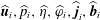 $\widehat{\boldsymbol{u}}_{i},\widehat{p}_{i},\widehat{\unicode[STIX]{x1D702}},\widehat{\unicode[STIX]{x1D711}}_{i},\widehat{\boldsymbol{j}}_{i},\widehat{\boldsymbol{b}}_{i}$
are identical to those defined in § 2.6.1 and capture all the magnetohydrodynamic effects related to surface elevation. The quasi-static corrections for the electrical potential and the current densities are related to either the vertical (superscripts
 $^{\mathit{v}}$
) or the horizontal magnetic field (superscript
 $^{\mathit{h}}$
). That is to say, we define the current density corrections as follows:
 $$\begin{eqnarray}\displaystyle \widehat{\boldsymbol{{\mathcal{J}}}}_{i}^{\mathit{v}} & = & \displaystyle \unicode[STIX]{x1D70E}_{i}(-\unicode[STIX]{x1D735}\widehat{\unicode[STIX]{x1D6F9}}_{i}^{\mathit{v}}+\widehat{\boldsymbol{u}}_{i}\times B_{z}\boldsymbol{e}_{z}),\end{eqnarray}$$
 $$\begin{eqnarray}\displaystyle \widehat{\boldsymbol{{\mathcal{J}}}}_{i}^{\mathit{h}} & = & \displaystyle \unicode[STIX]{x1D70E}_{i}(-\unicode[STIX]{x1D735}\widehat{\unicode[STIX]{x1D6F9}}_{i}^{\mathit{h}}+\widehat{\boldsymbol{u}}_{i}\times (\unicode[STIX]{x1D707}_{0}Jr/2)\boldsymbol{e}_{\unicode[STIX]{x1D703}}),\end{eqnarray}$$
 $\unicode[STIX]{x1D735}\boldsymbol{\cdot }\widehat{\boldsymbol{{\mathcal{J}}}}_{i}^{v}=\unicode[STIX]{x1D735}\boldsymbol{\cdot }\widehat{\boldsymbol{{\mathcal{J}}}}_{i}^{h}=0$
. This in turn implies that electrical potentials satisfy the following Laplace and Poisson problems:
 $$\begin{eqnarray}\unicode[STIX]{x1D6FB}^{2}\widehat{\unicode[STIX]{x1D6F9}}_{i}^{\mathit{v}}=0,\quad \unicode[STIX]{x1D6FB}^{2}\widehat{\unicode[STIX]{x1D6F9}}_{i}^{\mathit{h}}=-\unicode[STIX]{x1D707}_{0}J\widehat{u}_{z,i},\end{eqnarray}$$
with the following transmission and inhomogeneous boundary conditions:
 $$\begin{eqnarray}\left.\begin{array}{@{}c@{}}\widehat{\unicode[STIX]{x1D6F9}}_{1}^{\mathit{v}}|_{z=H_{1}}=0,\quad \unicode[STIX]{x2202}_{z}\widehat{\unicode[STIX]{x1D6F9}}_{2}^{\mathit{v}}|_{z=-H_{2}}=0,\quad \unicode[STIX]{x2202}_{r}\widehat{\unicode[STIX]{x1D6F9}}_{i}^{\mathit{v}}|_{r=R}=B_{z}\widehat{u}_{i,\unicode[STIX]{x1D703}}|_{r=R},\\ \widehat{\unicode[STIX]{x1D6F9}}_{1}^{\mathit{v}}|_{z=0}=\widehat{\unicode[STIX]{x1D6F9}}_{2}^{\mathit{v}}|_{z=0},\quad \unicode[STIX]{x1D70E}_{1}\unicode[STIX]{x2202}_{z}\widehat{\unicode[STIX]{x1D6F9}}_{1}^{\mathit{v}}|_{z=0}=\unicode[STIX]{x1D70E}_{2}\unicode[STIX]{x2202}_{z}\widehat{\unicode[STIX]{x1D6F9}}_{2}^{\mathit{v}}|_{z=0},\end{array}\right\}\end{eqnarray}$$
and
 $$\begin{eqnarray}\left.\begin{array}{@{}c@{}}\widehat{\unicode[STIX]{x1D6F9}}_{1}^{\mathit{h}}|_{z=H_{1}}=0,\quad \unicode[STIX]{x2202}_{z}\widehat{\unicode[STIX]{x1D6F9}}_{2}^{\mathit{h}}|_{z=-H_{2}}=(\unicode[STIX]{x1D707}_{0}Jr/2)\widehat{u}_{2,r}|_{z=-H_{2}},\\ \unicode[STIX]{x2202}_{r}\widehat{\unicode[STIX]{x1D6F9}}_{i}^{\mathit{h}}|_{r=R}=-(\unicode[STIX]{x1D707}_{0}JR/2)\widehat{u}_{i,z}|_{r=R},\quad \widehat{\unicode[STIX]{x1D6F9}}_{1}^{\mathit{h}}|_{z=0}=\widehat{\unicode[STIX]{x1D6F9}}_{2}^{\mathit{h}}|_{z=0},\\ \unicode[STIX]{x1D70E}_{1}(-\unicode[STIX]{x2202}_{z}\widehat{\unicode[STIX]{x1D6F9}}_{1}^{\mathit{h}}+(\unicode[STIX]{x1D707}_{0}Jr/2)\widehat{u}_{1,r})_{z=0}=\unicode[STIX]{x1D70E}_{2}(-\unicode[STIX]{x2202}_{z}\widehat{\unicode[STIX]{x1D6F9}}_{2}^{\mathit{h}}+(\unicode[STIX]{x1D707}_{0}Jr/2)\widehat{u}_{2,r})_{z=0}.\end{array}\right\}\end{eqnarray}$$
The problems defined here have no simple analytical solution, and below we discuss how we handle this in practice. Without any numerical calculation, we can deduce
 $$\begin{eqnarray}\left.\begin{array}{@{}c@{}}{\displaystyle \frac{\{\widehat{\unicode[STIX]{x1D6F9}}_{i}^{\mathit{h}},\widehat{{\mathcal{J}}}_{i,r}^{\mathit{h}},\widehat{{\mathcal{J}}}_{i,z}^{\mathit{h}},\widehat{{\mathcal{J}}}_{i,\unicode[STIX]{x1D703}}^{\mathit{v}},\widehat{{\mathcal{B}}}_{i,r}^{\mathit{v}},\widehat{{\mathcal{B}}}_{i,z}^{\mathit{v}},\widehat{{\mathcal{B}}}_{i,\unicode[STIX]{x1D703}}^{\mathit{h}}\}}{A\exp (\text{i}m\unicode[STIX]{x1D703})}}\in \mathbb{R},\\ {\displaystyle \frac{\{\widehat{\unicode[STIX]{x1D6F9}}_{i}^{\mathit{v}},\widehat{{\mathcal{J}}}_{i,r}^{\mathit{v}},\widehat{{\mathcal{J}}}_{i,z}^{\mathit{v}},\widehat{{\mathcal{J}}}_{i,\unicode[STIX]{x1D703}}^{\mathit{h}},\widehat{{\mathcal{B}}}_{i,r}^{\mathit{h}},\widehat{{\mathcal{B}}}_{i,z}^{\mathit{h}},\widehat{{\mathcal{B}}}_{i,\unicode[STIX]{x1D703}}^{\mathit{v}}\}}{A\exp (\text{i}m\unicode[STIX]{x1D703})}}\in \text{i}\mathbb{R}.\end{array}\right\}\end{eqnarray}$$
Let us briefly suppose that the quasi-static field corrections are known and pursue the calculations to find the impact on
 $\unicode[STIX]{x1D6FC}$
, the complex frequency shift. In this augmented, quasi-static version of the problem, we find a modified solvability condition,
 $$\begin{eqnarray}\displaystyle & & \displaystyle \mathop{\sum }_{i=1,2}\int _{V_{i}}[\widehat{\boldsymbol{u}}_{i}^{\ast }\boldsymbol{\cdot }(\unicode[STIX]{x1D6FC}\unicode[STIX]{x1D70C}_{i}\widehat{\boldsymbol{u}}_{i}+\text{i}\unicode[STIX]{x1D714}\unicode[STIX]{x1D70C}_{i}\widetilde{\boldsymbol{u}}_{i}+\unicode[STIX]{x1D735}\widetilde{p}_{i})+\widehat{p}_{i}^{\ast }\unicode[STIX]{x1D735}\boldsymbol{\cdot }\widetilde{\boldsymbol{u}}_{i}]\,\text{d}V\nonumber\\ \displaystyle & & \displaystyle \quad =\mathop{\sum }_{i=1,2}\int _{V_{i}}\widehat{\boldsymbol{u}}_{i}^{\ast }\boldsymbol{\cdot }\left[(\widehat{\boldsymbol{j}}_{i}+\widehat{\boldsymbol{{\mathcal{J}}}}_{i}^{\mathit{v}}+\widehat{\boldsymbol{{\mathcal{J}}}}_{i}^{\mathit{h}})\times \boldsymbol{B}+\boldsymbol{J}\times (\widehat{\boldsymbol{b}}_{i}+\widehat{\boldsymbol{{\mathcal{B}}}}_{i}^{\mathit{v}}+\widehat{\boldsymbol{{\mathcal{B}}}}_{i}^{\mathit{h}})\right]\,\text{d}V.\end{eqnarray}$$
Similar simplifications as before lead to a new formula for the complex frequency shift
 $$\begin{eqnarray}\unicode[STIX]{x1D6FC}=\underbrace{\frac{{\mathcal{P}}_{\mathit{v}}}{2{\mathcal{K}}}}_{\unicode[STIX]{x1D706}_{\mathit{v}}}+\underbrace{\frac{{\mathcal{Q}}_{\mathit{vv}}}{2{\mathcal{K}}}}_{\unicode[STIX]{x1D706}_{\mathit{vv}}}+\underbrace{\frac{{\mathcal{Q}}_{\mathit{hh}}}{2{\mathcal{K}}}}_{\unicode[STIX]{x1D706}_{\mathit{hh}}}+\underbrace{\frac{{\mathcal{P}}_{\mathit{h}}}{2{\mathcal{K}}}}_{\text{i}\unicode[STIX]{x1D6FF}_{\mathit{v}}}+\underbrace{\frac{{\mathcal{Q}}_{\mathit{vh}}}{2{\mathcal{K}}}}_{\text{i}\unicode[STIX]{x1D6FF}_{\mathit{vh}}},\end{eqnarray}$$
with
 ${\mathcal{K}},{\mathcal{P}}_{v},{\mathcal{P}}_{h}$
as before and
 $$\begin{eqnarray}\displaystyle {\mathcal{Q}}_{\mathit{vv}} & = & \displaystyle \mathop{\sum }_{i=1,2}\int _{V_{i}}\widehat{\boldsymbol{u}}_{i}^{\ast }\boldsymbol{\cdot }\left(\widehat{\boldsymbol{{\mathcal{J}}}}_{i}^{\mathit{v}}\times B_{z}\boldsymbol{e}_{z}\right)\text{d}V,\end{eqnarray}$$
 $$\begin{eqnarray}\displaystyle {\mathcal{Q}}_{\mathit{hh}} & = & \displaystyle \mathop{\sum }_{i=1,2}\int _{V_{i}}\left\{\widehat{\boldsymbol{u}}_{i}^{\ast }\boldsymbol{\cdot }\left[\widehat{\boldsymbol{{\mathcal{J}}}}_{i}^{\mathit{h}}\times (\unicode[STIX]{x1D707}_{0}Jr/2)\boldsymbol{e}_{\unicode[STIX]{x1D703}}\right]+\unicode[STIX]{x1D707}_{0}J\widehat{\unicode[STIX]{x1D719}}_{i}^{\ast }\,\widehat{{\mathcal{J}}}_{i,z}^{\mathit{h}}\right\}\,\text{d}V,\end{eqnarray}$$
 $$\begin{eqnarray}\displaystyle {\mathcal{Q}}_{\mathit{vh}} & = & \displaystyle \mathop{\sum }_{i=1,2}\int _{V_{i}}\left\{\widehat{\boldsymbol{u}}_{i}^{\ast }\boldsymbol{\cdot }\left[\widehat{\boldsymbol{{\mathcal{J}}}}_{i}^{\mathit{h}}\times B_{z}\boldsymbol{e}_{z}+\widehat{\boldsymbol{{\mathcal{J}}}}_{i}^{\mathit{v}}\times (\unicode[STIX]{x1D707}_{0}Jr/2)\boldsymbol{e}_{\unicode[STIX]{x1D703}}\right]+\unicode[STIX]{x1D707}_{0}J\widehat{\unicode[STIX]{x1D719}}_{i}^{\ast }\,\widehat{{\mathcal{J}}}_{i,z}^{\mathit{v}}\right\}\,\text{d}V.\quad\end{eqnarray}$$
 ${\mathcal{Q}}_{\mathit{hh}}$
and
 ${\mathcal{Q}}_{\mathit{vh}}$
, but does not affect
 ${\mathcal{Q}}_{\mathit{vv}}$
. Using the real and imaginary character of the fields (2.53), we readily deduce that
 ${\mathcal{Q}}_{\mathit{vv}},{\mathcal{Q}}_{\mathit{hh}}$
are real whereas
 ${\mathcal{Q}}_{\mathit{vh}}$
is imaginary, thus yielding the quasi-static corrections
 $\unicode[STIX]{x1D706}_{\mathit{vv}},\unicode[STIX]{x1D706}_{\mathit{hh}}$
to the growth rate
 $\unicode[STIX]{x1D706}_{\mathit{v}}$
and the quasi-static correction
 $\unicode[STIX]{x1D6FF}_{\mathit{vh}}$
to the frequency shift
 $\unicode[STIX]{x1D6FF}_{h}$
.
In practice, we still need to solve for the fields
 $\widehat{\unicode[STIX]{x1D6F9}}_{i}^{v}$
and
 $\widehat{\unicode[STIX]{x1D6F9}}_{i}^{\mathit{h}}$
to be able to evaluate these integrals and here we have chosen two different approaches. The first approach is adapted to arbitrary values of
 $\unicode[STIX]{x1D70E}_{i}$
: we just calculate
 $\widehat{\unicode[STIX]{x1D6F9}}_{i}^{v}$
and
 $\widehat{\unicode[STIX]{x1D6F9}}_{i}^{\mathit{h}}$
numerically solving the mentioned Laplace and Poisson problems. We use a Fourier expansion in the azimuthal direction; that is, we set
 $\widehat{\unicode[STIX]{x1D6F9}}_{i}^{\mathit{v}}=f_{i}^{\mathit{v}}(r,z)\exp (\text{i}m\unicode[STIX]{x1D703})$
,
 $\widehat{\unicode[STIX]{x1D6F9}}_{i}^{\mathit{h}}=f_{i}^{\mathit{h}}(r,z)\exp (\text{i}m\unicode[STIX]{x1D703})$
, and we solve the two-dimensional problems for
 $f_{i}^{\mathit{v}}$
and
 $f_{i}^{\mathit{h}}$
using a standard second-order finite-difference method on a uniform grid with
 $2\times (M+1)^{2}$
points,
 $$\begin{eqnarray}\left\{\begin{array}{@{}l@{}}\text{region 1:}\quad (i\unicode[STIX]{x1D6FF}r,j\unicode[STIX]{x1D6FF}z_{1}),\quad \\ \text{region 2:}\quad (i\unicode[STIX]{x1D6FF}r,-j\unicode[STIX]{x1D6FF}z_{2}),\quad \end{array}\right.\quad \forall i,j\in \{0,1,\ldots ,M\}.\end{eqnarray}$$
Here
 $\unicode[STIX]{x1D6FF}r=R/M$
,
 $\unicode[STIX]{x1D6FF}z_{1}=H_{1}/M$
,
 $\unicode[STIX]{x1D6FF}z_{2}=H_{2}/M$
. Radial and vertical derivatives appearing in the boundary conditions are discretized using second-order uncentred finite-difference formulas. At the axis, we enforce the regularity condition
 $\widehat{\unicode[STIX]{x1D6F9}}_{i}^{\mathit{v}}|_{r=0}=\widehat{\unicode[STIX]{x1D6F9}}_{i}^{\mathit{h}}|_{r=0}=0$
for
 $m\neq 0$
.
 ${\mathcal{Q}}_{\mathit{vv}}$
,
 ${\mathcal{Q}}_{\mathit{hh}}$
,
 ${\mathcal{Q}}_{\mathit{vh}}$
are then calculated numerically using the field profiles provided by the finite-difference code, using a simple trapezoidal quadrature.
The need to use a numerical approach to find the quasi-static corrections is slightly unsatisfying. Therefore we also propose a second approach applicable to the realistic limit where
 $\unicode[STIX]{x1D70E}_{1}\ll \unicode[STIX]{x1D70E}_{2}$
. In that case, the induction in the top cryolite layer is very weak, and we can use the approximation
 $$\begin{eqnarray}\widehat{\boldsymbol{{\mathcal{J}}}}_{1}^{\mathit{v}}\approx \widehat{\boldsymbol{{\mathcal{J}}}}_{1}^{\mathit{h}}\approx \mathbf{0}.\end{eqnarray}$$
We then need to solve (2.50) in the bottom aluminium layer only, with the boundary conditions stated in (2.51), (2.52), and the transmission conditions replaced by
 $$\begin{eqnarray}\unicode[STIX]{x2202}_{z}\widehat{\unicode[STIX]{x1D6F9}}_{2}^{\mathit{v}}|_{z=0}\approx 0,\quad \unicode[STIX]{x2202}_{z}\widehat{\unicode[STIX]{x1D6F9}}_{2}^{\mathit{h}}|_{z=0}\approx (\unicode[STIX]{x1D707}_{0}Jr/2)\widehat{u}_{2,r}|_{z=0}.\end{eqnarray}$$
Analytical solutions can be obtained in terms of a series of harmonic functions. The calculation for
 $\widehat{\unicode[STIX]{x1D6F9}}_{2}^{\mathit{h}}$
is quite tedious and is not presented here for brevity. The computation for
 $\widehat{\unicode[STIX]{x1D6F9}}_{2}^{\mathit{v}}$
is easier and we can propose
 $$\begin{eqnarray}\widehat{\unicode[STIX]{x1D6F9}}_{2}^{\mathit{v}}=\left[C_{0}\left(\frac{r}{R}\right)^{m}+\mathop{\sum }_{j=1}^{+\infty }C_{j}\text{I}_{m}(j\unicode[STIX]{x03C0}r/H_{2})\cos (j\unicode[STIX]{x03C0}z/H_{2})\right]\text{e}^{\text{i}m\unicode[STIX]{x1D703}},\end{eqnarray}$$
as a candidate harmonic solution. Here
 $\text{I}_{m}$
is a modified Bessel function. The coefficients
 $C_{0},C_{1},C_{2},\ldots$
are calculated by projecting the inhomogeneous boundary condition
 $\unicode[STIX]{x2202}_{r}\widehat{\unicode[STIX]{x1D6F9}}_{2}^{\mathit{v}}|_{r=R}=\widehat{u}_{\unicode[STIX]{x1D703},2}|_{r=R}B_{z}$
onto the set of the basis functions
 $\{\cos (j\unicode[STIX]{x03C0}z/H_{2}),j\in \mathbb{N}\}$
using the orthogonality relation
 $$\begin{eqnarray}\int _{-H_{2}}^{0}\cos \frac{j\unicode[STIX]{x03C0}z}{H_{2}}\cos \frac{j^{\prime }\unicode[STIX]{x03C0}z}{H_{2}}=\unicode[STIX]{x1D6FF}_{j,j^{\prime }}\left\{\begin{array}{@{}ll@{}}H_{2},\quad & j=0\\ H_{2}/2,\quad & j\neq 0.\end{array}\right.\end{eqnarray}$$
This yields
 $$\begin{eqnarray}\left.\begin{array}{@{}c@{}}C_{0}=-\text{i}{\displaystyle \frac{\unicode[STIX]{x1D714}ARB_{z}}{k^{2}H_{2}}}\text{J}_{m}(kR),\\ C_{j}=-\text{i}{\displaystyle \frac{\unicode[STIX]{x1D714}ARB_{z}}{kj\unicode[STIX]{x03C0}}}{\displaystyle \frac{4m\text{J}_{m}(kR)}{(kR)(I_{m+1}(j\unicode[STIX]{x03C0}R/H_{2})+I_{m-1}(j\unicode[STIX]{x03C0}R/H_{2}))}}{\displaystyle \frac{k^{2}}{k^{2}+(j\unicode[STIX]{x03C0}/H_{2})^{2}}}\sinh (kH_{2}).\end{array}\right\}\end{eqnarray}$$
With this information we know
 $\widehat{\unicode[STIX]{x1D6F9}}_{2}^{\mathit{v}}$
and so we can calculate the integral
 ${\mathcal{Q}}_{\mathit{vv}}$
ignoring contributions from the top layer. This integral can be rewritten as
 $$\begin{eqnarray}{\mathcal{Q}}_{\mathit{vv}}\approx -\unicode[STIX]{x1D70E}_{2}\int _{V_{2}}\Vert \widehat{\boldsymbol{u}}_{2}^{\ast }\times B_{z}\boldsymbol{e}_{z}\Vert ^{2}\,\text{d}V+\int _{V_{2}}\widehat{\boldsymbol{u}}_{2}^{\ast }\boldsymbol{\cdot }\left(-\unicode[STIX]{x1D70E}_{2}\unicode[STIX]{x1D735}\widehat{\unicode[STIX]{x1D6F9}}_{2}^{\mathit{v}}\times B_{z}\boldsymbol{e}_{z}\right)\text{d}V.\end{eqnarray}$$
In containers with perfectly conducting side walls, we would have
 $\widehat{\unicode[STIX]{x1D6F9}}_{2}^{\mathit{v}}=0$
and only the first term would then contribute. Here the side walls are insulating and therefore
 $\widehat{\unicode[STIX]{x1D6F9}}_{2}^{\mathit{v}}\neq 0$
. This second term can drastically reduce the magnetic damping as explained by Sreenivasan, Davidson & Etay (Reference Sreenivasan, Davidson and Etay2005) and should certainly not be ignored. Analytical evaluation of all the integrals finally yields the following formula
 $$\begin{eqnarray}\displaystyle \unicode[STIX]{x1D706}_{\mathit{vv}} & = & \displaystyle {\mathcal{Q}}_{\mathit{vv}}/2{\mathcal{K}}\nonumber\\ \displaystyle & {\approx} & \displaystyle \frac{\unicode[STIX]{x1D70E}_{2}B_{z}^{2}}{{\displaystyle \frac{\unicode[STIX]{x1D70C}_{1}}{\tanh (kH_{1})}}+{\displaystyle \frac{\unicode[STIX]{x1D70C}_{2}}{\tanh (kH_{2})}}}\left\{-\frac{1}{4}\left({\displaystyle \frac{1}{\tanh (kH_{2})}}+{\displaystyle \frac{kH_{2}}{\sinh ^{2}(kH_{2})}}\right)+\left(\frac{1}{k^{2}R^{2}-m^{2}}\right)\right.\nonumber\\ \displaystyle & & \displaystyle \times \left.\left[\frac{m}{kH_{2}}+4m^{2}\mathop{\sum }_{j=1}^{+\infty }\left(\frac{1}{j\unicode[STIX]{x03C0}}\right)\!\frac{k^{3}}{R(k^{2}+(j\unicode[STIX]{x03C0}/H_{2})^{2})^{2}}\frac{\text{I}_{m}(j\unicode[STIX]{x03C0}R/H_{2})}{I_{m+1}(j\unicode[STIX]{x03C0}R/H_{2})+I_{m-1}(j\unicode[STIX]{x03C0}R/H_{2})}\!\right]\!\right\}.\nonumber\\ \displaystyle & & \displaystyle\end{eqnarray}$$
In the infinite sum over
 $j$
, we observe a fast exponential decay of the terms and the shallower the cell, the faster the decay. All the computations reported in the paper are done by truncating the sum over
 $j$
to the first 50 terms. Below we successfully compare this formula to the numerical finite-difference approach. In the shallow limit,
 $kH_{i}\ll 1$
, a single term is dominant and yields
 $$\begin{eqnarray}\unicode[STIX]{x1D706}_{\mathit{vv},\mathit{shallow}}\approx \frac{\unicode[STIX]{x1D70E}_{2}B_{z}^{2}}{\unicode[STIX]{x1D70C}_{1}\left({\displaystyle \frac{H_{2}}{H_{1}}}\right)+\unicode[STIX]{x1D70C}_{2}}\left(-\frac{1}{2}+\frac{m}{k^{2}R^{2}-m^{2}}\right)\end{eqnarray}$$
for the magnetic damping caused by the vertical magnetic field. No significant simplification occurs in (2.64) in the deep limit
 $kH_{i}\gg 1$
because the cosine basis used in the expansion is not adapted to the infinitely deep case.
2.6.3 Viscous corrections: damping
$\unicode[STIX]{x1D706}_{\mathit{visc}}$
, frequency shift
$\unicode[STIX]{x1D6FF}_{\mathit{visc}}$


We finally include the viscous effects. To leading order we can ignore all magnetohydrodynamic effects. Viscosity will act on the waves just as in a purely hydrodynamic set-up. The earliest calculations of viscous damping rates of waves in cylinders filled with one fluid go back to Case & Parkinson (Reference Case and Parkinson1957), but no explicit formula is available for the case of two fluid layers. In appendix D we detail our calculation of the viscous effects on gravity waves. First, we find the leading-order spatial structure of the viscous boundary layers (Stokes layers). Near the solid walls, these boundary layers resemble those we can find in a cylinder filled with one liquid. Different is that, near the interface between both liquids, a viscous boundary layer is required to ensure the continuity of the flow field and that of the tangential viscous stress. By extending the method of Case & Parkinson (Reference Case and Parkinson1957) to the two-layer case, we then calculate the viscous damping rates from a perturbative expansion on the mechanical energy balance. A second, alternative approach, passes by a solvability condition. It confirms the formula for the viscous damping rate and also provides access to the frequency shift caused by viscosity. Our formulas are only valid for a freely sliding contact line making an angle of
 $90^{\circ }$
with the solid wall and we ignore contact line hysteresis (see Viola & Gallaire Reference Viola and Gallaire2018) and suppose an unpolluted interface. We find
 $$\begin{eqnarray}\unicode[STIX]{x1D706}_{\mathit{visc}}=\unicode[STIX]{x1D706}_{\mathit{visc}}^{s}+\unicode[STIX]{x1D706}_{\mathit{visc}}^{i},\quad \unicode[STIX]{x1D6FF}_{\mathit{visc}}=\text{Sgn}(\unicode[STIX]{x1D714})\unicode[STIX]{x1D706}_{\mathit{visc}},\end{eqnarray}$$
with
 $$\begin{eqnarray}\unicode[STIX]{x1D706}_{\mathit{visc}}^{s}=-\frac{1}{2\sqrt{2}}\mathop{\sum }_{i=1,2}\frac{\sqrt{{\displaystyle \frac{\unicode[STIX]{x1D708}_{i}|\unicode[STIX]{x1D714}|}{R^{2}}}}\unicode[STIX]{x1D70C}_{i}\left[{\displaystyle \frac{k(R-H_{i})}{\sinh ^{2}(kH_{i})}}+\left({\displaystyle \frac{k^{2}R^{2}+m^{2}}{k^{2}R^{2}-m^{2}}}\right){\displaystyle \frac{1}{\tanh (kH_{i})}}\right]}{\left[{\displaystyle \frac{\unicode[STIX]{x1D70C}_{1}}{\tanh (kH_{1})}}+{\displaystyle \frac{\unicode[STIX]{x1D70C}_{2}}{\tanh (kH_{2})}}\right]}\end{eqnarray}$$
and
 $$\begin{eqnarray}\unicode[STIX]{x1D706}_{\mathit{visc}}^{i}=-\frac{\sqrt{|\unicode[STIX]{x1D714}|}k}{2\sqrt{2}}\frac{\left[{\displaystyle \frac{1}{\tanh (kH_{1})}}+{\displaystyle \frac{1}{\tanh (kH_{2})}}\right]^{2}}{\left[{\displaystyle \frac{\unicode[STIX]{x1D70C}_{1}}{\tanh (kH_{1})}}+{\displaystyle \frac{\unicode[STIX]{x1D70C}_{2}}{\tanh (kH_{2})}}\right]\left({\displaystyle \frac{1}{\unicode[STIX]{x1D70C}_{1}\sqrt{\unicode[STIX]{x1D708}_{1}}}}+{\displaystyle \frac{1}{\unicode[STIX]{x1D70C}_{2}\sqrt{\unicode[STIX]{x1D708}_{2}}}}\right)}.\end{eqnarray}$$
The term
 $\unicode[STIX]{x1D706}_{\mathit{visc}}^{s}$
relates to viscous dissipation caused in boundary layers near solid walls, whereas the term
 $\unicode[STIX]{x1D706}_{\mathit{visc}}^{i}$
is caused by the boundary layers at the interface. Both terms can have comparable magnitudes in liquids with similar densities and kinematic viscosities. A much weaker higher-order damping term (often referred to as the interior damping term) is here ignored, but is calculated in appendix D. In the limit of one fluid layer,
 $\unicode[STIX]{x1D70C}_{1}\rightarrow 0$
, we recover the known damping rates (Case & Parkinson Reference Case and Parkinson1957; Ibrahim Reference Ibrahim2005). In the shallow limit
 $kH_{i}\ll 1$
, we can derive the asymptotic form
 $$\begin{eqnarray}\displaystyle \unicode[STIX]{x1D706}_{\mathit{visc},\mathit{shallow}}^{s} & {\approx} & \displaystyle -\frac{1}{2\sqrt{2}}\frac{\unicode[STIX]{x1D70C}_{1}H_{1}^{-2}\sqrt{\unicode[STIX]{x1D708}_{1}}+\unicode[STIX]{x1D70C}_{2}H_{2}^{-2}\sqrt{\unicode[STIX]{x1D708}_{2}}}{\unicode[STIX]{x1D70C}_{1}H_{1}^{-1}+\unicode[STIX]{x1D70C}_{2}H_{2}^{-1}}\sqrt{|\unicode[STIX]{x1D714}_{\mathit{shallow}}|},\end{eqnarray}$$
 $$\begin{eqnarray}\displaystyle \unicode[STIX]{x1D706}_{\mathit{visc},\mathit{shallow}}^{i} & {\approx} & \displaystyle -\frac{1}{2\sqrt{2}}\frac{(H_{1}^{-1}+H_{2}^{-1})^{2}}{(\unicode[STIX]{x1D70C}_{1}H_{1}^{-1}+\unicode[STIX]{x1D70C}_{2}H_{2}^{-1})\left({\displaystyle \frac{1}{\unicode[STIX]{x1D70C}_{1}\sqrt{\unicode[STIX]{x1D708}_{1}}}}+{\displaystyle \frac{1}{\unicode[STIX]{x1D70C}_{2}\sqrt{\unicode[STIX]{x1D708}_{2}}}}\right)}\sqrt{|\unicode[STIX]{x1D714}_{\mathit{shallow}}|},\end{eqnarray}$$
 $kH_{i}\gg 1$
, we can use
 $$\begin{eqnarray}\displaystyle \unicode[STIX]{x1D706}_{\mathit{visc},\mathit{deep}}^{s} & {\approx} & \displaystyle -\frac{1}{2\sqrt{2}}\left({\displaystyle \frac{k^{2}R^{2}+m^{2}}{k^{2}R^{2}-m^{2}}}\right)\frac{1}{R}\frac{\unicode[STIX]{x1D70C}_{1}\sqrt{\unicode[STIX]{x1D708}_{1}}+\unicode[STIX]{x1D70C}_{2}\sqrt{\unicode[STIX]{x1D708}_{2}}}{\unicode[STIX]{x1D70C}_{1}+\unicode[STIX]{x1D70C}_{2}}\sqrt{|\unicode[STIX]{x1D714}_{\mathit{deep }}|},\end{eqnarray}$$
 $$\begin{eqnarray}\displaystyle \unicode[STIX]{x1D706}_{\mathit{visc},\mathit{deep}}^{i} & {\approx} & \displaystyle -\sqrt{2}k\left[(\unicode[STIX]{x1D70C}_{1}+\unicode[STIX]{x1D70C}_{2})\left({\displaystyle \frac{1}{\unicode[STIX]{x1D70C}_{1}\sqrt{\unicode[STIX]{x1D708}_{1}}}}+{\displaystyle \frac{1}{\unicode[STIX]{x1D70C}_{2}\sqrt{\unicode[STIX]{x1D708}_{2}}}}\right)\right]^{-1}\sqrt{|\unicode[STIX]{x1D714}_{\mathit{deep }}|}\end{eqnarray}$$
3 Experimental validation of viscous damping rate formula
Using the orbital sloshing device fully described in Horstmann et al. (Reference Horstmann, Wylega and Weier2019), we have been able to measure viscous damping rates of gravity waves in two-fluid systems. A sketch of the set-up is shown in figure 3. We use a polished acrylic glass container with radius
 $R=5~\text{cm}$
and total height
 $H_{1}+H_{2}=10~\text{cm}$
. Both the top and bottom caps of the cylinder have ten supply holes uniformly distributed on a circle at 42 mm from the vertical axis. These holes are used to attach up to ten ultrasound probes. A small layer of acrylic glass 5 mm thick is kept between the probes and the observation volume to ensure non-invasive ultrasound measurements of the interfacial motion. The upper cap additionally contains a small filling hole of diameter 4 mm to degas the cell and to adjust the position of the interface. The cylinder is placed on a sample holder to facilitate ultrasound measurements also from below. This way, up to 20 ultrasound probes can be simultaneously employed making it possible to precisely reconstruct the motion of the interface. The measurements have been done with the Ultrasound Doppler Velocimeter DOP 3010 from Signal-Processing. By directly identifying and tracking the ultrasound echo reflected by the interface, the interfacial wave motion can be precisely measured for wave amplitudes in the range (0.15 mm, 10 mm). Finally, the sample holder is mounted onto a Kuhner LS-X lab-shaking table
 $(420\times 420~\text{mm})$
, which can prescribe ideal circular motions to the vessel, parameterized as follows:
 $$\begin{eqnarray}\boldsymbol{r}_{orbital}(t)=\frac{d_{s}}{2}(\cos (\unicode[STIX]{x1D6FA}t)\boldsymbol{e}_{x}+\sin (\unicode[STIX]{x1D6FA}t)\boldsymbol{e}_{y}).\end{eqnarray}$$
We denote
 $\unicode[STIX]{x1D6FA}$
the shaking frequency and
 $d_{s}$
the diameter of the circular motion of the vertical axis of the vessel. The shaker is designed to allow for a continuous adjustment of the shaking diameter up to
 $d_{s}=70~\text{mm}$
and to set shaking frequencies from
 $\unicode[STIX]{x1D6FA}=20$
up to
 $\unicode[STIX]{x1D6FA}=500~\text{min}^{-1}$
in steps of
 $1~\text{min}^{-1}$
. The cylinder is filled with two different transparent fluids. We use a top layer composed of Paraffinum Perliquidum (
 $\unicode[STIX]{x1D70C}_{1}=0.846~\text{g}~\text{cm}^{-3}$
,
 $\unicode[STIX]{x1D708}_{1}=36~\text{mm}^{2}~\text{s}^{-1}$
,
 $\unicode[STIX]{x1D6FE}_{1|air}\approx 30~\text{mN}~\text{m}^{-1}$
), and the bottom layer is composed of Wacker® silicone oil AK 35 (
 $\unicode[STIX]{x1D70C}_{2}=0.955~\text{g}~\text{cm}^{-3}$
,
 $\unicode[STIX]{x1D708}_{2}=35~\text{mm}^{2}~\text{s}^{-1}$
,
 $\unicode[STIX]{x1D6FE}_{2|air}=20.7~\text{mN}~\text{m}^{-1}$
). This combination of fluids realizes a very good approximation of the idealized boundary condition that are used in this study: no meniscus was visible and we observed an almost free-sliding contact line. We measured a surface tension
 $\unicode[STIX]{x1D6FE}_{1|2}\leqslant 25~\text{mN}~\text{m}^{-1}$
at the interface between both liquids and this implies that capillary effects may be ignored in this experiment.
Experimental set-up used to measure viscous wave damping and typical signal. A cylinder filled with a layer of Paraffinum Perliquidum and a layer of silicone oil is put on an orbital shaker. A rotating gravity wave is driven on the interface. When impulsively stopped, the gravity wave decays and we measure the viscous damping rates of the wave amplitude in the Doppler probe signals.

Orbital motion causes a large-scale rotating wave
 $(m,n)=(1,1)$
, which also is the wave that is most frequently associated with the metal pad roll instability. We used the following strict protocol to measure the experimental damping rate of this wave. Pre-measurements were conducted to find the experimental eigenfrequency
 $\unicode[STIX]{x1D6FA}$
of the mode
 $(m,n)=(1,1)$
for each choice of
 $H_{2}$
, since it is known from Reclari et al. (Reference Reclari, Dreyer, Tissot, Obreschkow, Wurm and Farhat2014) that at resonance the forced wave motion is close to that of free gravity waves. We then drive the rotating wave at the resonant frequency, and adjust the shaking diameter
 $d_{s}$
so that the wave is large enough to allow measurements of the damping rate but is small enough to remain in the linear, non-breaking wave regime (amplitudes between 3 mm and 5 mm in practice). The table is turned off after the wave has settled in a saturated state. Subsequently, we give the wave some time (approximately one up to two periods) to become a ‘free’ gravity wave. Then the exponential decay rate
 $-\unicode[STIX]{x1D706}$
is determined by fitting the measured wave amplitude with the ansatz
 $$\begin{eqnarray}A(t)\approx A_{0}\text{e}^{\unicode[STIX]{x1D706}t}\cos (\unicode[STIX]{x1D6FA}t-\unicode[STIX]{x1D709}).\end{eqnarray}$$
Here
 $A_{0}$
and
 $\unicode[STIX]{x1D709}$
denote the initial wave amplitude and phase that also need to be fitted, which introduces some uncertainty.
In figure 4 we compare the measured damping rates to the theoretical formulas (2.66)–(2.68), for varying
 $H_{2}$
and
 $H_{1}=10~\text{cm}-H_{2}$
. Error bars were estimated by using different fitting time intervals. The measured decay rates are in very good agreement with the theoretical viscous damping rate, although the theory seems to underestimate slightly the measured damping rates. Figure 4 also shows the theoretical damping rates in the shallow and deep limits. The measurements coincide with the deep limit when
 $H_{1}=H_{2}=5~\text{cm}$
, and they coincide with the shallow limit when either
 $H_{1}\ll H_{2}$
or
 $H_{1}\gg H_{2}$
. In conclusion we have compared the damping rates in the full transitional regime between these simplified asymptotic limits which are frequently analysed in the literature. Our theory suitably predicts the viscous damping rates of gravity waves of two-layer systems when the simplified boundary conditions at the contact line are fulfilled.
Measured damping rates
 $\unicode[STIX]{x1D706}$
are compared with the theoretical viscous damping rates from (2.66) for different interfacial heights
 $H_{2}$
keeping
 $H_{1}+H_{2}=10~\text{cm}$
. The theoretical damping rates in the shallow limit (2.67) and the theoretical damping rates in the deep limit (2.68) are also shown.

4 Numerical validation of the theory in a small-scale reduction cell
Flueck et al. (Reference Flueck, Hofer, Picasso, Rappaz and Steiner2009) and Steiner (Reference Steiner2009) numerically simulate the metal pad roll instability in a small cylindrical reduction cell with dimensions
 $$\begin{eqnarray}R=0.035~\text{m},\quad (H_{1},H_{2})=(0.075~\text{m},0.075~\text{m}).\end{eqnarray}$$
Compared to industrial Hall–Héroult cells, this cell is non-shallow and tiny but it has the advantage that high accuracy numerical simulations are feasible. Such direct simulations are done here and from them, we can obtain numerical measurements that allow a detailed comparison with our theoretical model. We use the material properties of the cryolite and aluminium
 $$\begin{eqnarray}\left.\begin{array}{@{}c@{}}(\unicode[STIX]{x1D70C}_{1},\unicode[STIX]{x1D70C}_{2})=(2150,2300)~\text{kg}~\text{m}^{-3},\\ (\unicode[STIX]{x1D70E}_{1},\unicode[STIX]{x1D70E}_{2})=(250,3.5\times 10^{6})~\text{S}~\text{m}^{-1},\\ (\unicode[STIX]{x1D708}_{1},\unicode[STIX]{x1D708}_{2})=(1.2,0.52)\times 10^{-6}~\text{m}^{2}~\text{s}^{-1}.\end{array}\right\}\end{eqnarray}$$
We keep
 $J\in [0,15]\times 10^{4}~\text{A}~\text{m}^{-2}$
within realistic levels but for the external field
 $B_{z}$
, we take the liberty of imposing very high magnetic fields
 $B_{z}$
up to
 $16~\text{mT}$
, just as Flueck et al. (Reference Flueck, Hofer, Picasso, Rappaz and Steiner2009), Steiner (Reference Steiner2009) or similar to what was done in the experimental devices of Pedchenko et al. (Reference Pedchenko, Molokov, Priede, Lukyanov and Thomas2009, Reference Pedchenko, Molokov and Bardet2017). Surface tension will be absent
 $\unicode[STIX]{x1D6FE}_{1|2}=0$
or present
 $\unicode[STIX]{x1D6FE}_{1|2}=0.5~\text{N}~\text{m}^{-1}$
(value from Steiner (Reference Steiner2009)).
Theoretical values for all the quantities characterizing the growth rate and frequency of various waves
 $(m,n)$
in the small cell. Superscript (a), without surface tension
 $\unicode[STIX]{x1D6FE}_{1|2}=0$
, superscript (b) with surface tension
 $\unicode[STIX]{x1D6FE}_{1|2}=0.5~\text{N}~\text{m}^{-1}$
.
 $\unicode[STIX]{x1D706}_{\mathit{vv}}$
and the ratio
 $\unicode[STIX]{x1D706}_{\mathit{visc}}^{i}/\unicode[STIX]{x1D706}_{\mathit{visc}}$
are independent of
 $\unicode[STIX]{x1D6FE}_{1|2}$
. All the quantities are in MKS units:
 $k$
in
 $\text{m}^{-1}$
,
 $J$
in
 $\text{A}~\text{m}^{-2}$
,
 $B_{z}$
in T,
 $\unicode[STIX]{x1D714}$
,
 $\unicode[STIX]{x1D706}_{\mathit{v}}$
,
 $\unicode[STIX]{x1D706}_{\mathit{vv}}$
,
 $\unicode[STIX]{x1D706}_{\mathit{visc}}$
in
 $\text{s}^{-1}$
.

4.1 Theoretical predictions
Due to its small radius, limited
 $J$
and relatively high
 $B_{z}$
, the horizontal magnetic field is negligible:
 $B_{\unicode[STIX]{x1D703}}=\unicode[STIX]{x1D707}_{0}Jr/2\ll B_{z}$
. As a result, we obtain a very good approximation for the growth rate and frequency shift with
 $$\begin{eqnarray}\unicode[STIX]{x1D706}\approx \unicode[STIX]{x1D706}_{\mathit{v}}+\unicode[STIX]{x1D706}_{\mathit{vv}}+\unicode[STIX]{x1D706}_{\mathit{visc}},\quad \unicode[STIX]{x1D6FF}\approx \unicode[STIX]{x1D6FF}_{\mathit{visc}}.\end{eqnarray}$$
Table 1 provides numerical values obtained from our theory (in SI units) for the wavenumbers
 $k$
and the frequencies
 $\unicode[STIX]{x1D714}$
of several waves
 $(m,n)$
together with
 $\unicode[STIX]{x1D706}_{\mathit{v}}/JB_{z}$
,
 $\unicode[STIX]{x1D706}_{\mathit{vv}}/B_{z}^{2}$
,
 $\unicode[STIX]{x1D706}_{\mathit{visc}}(=\unicode[STIX]{x1D6FF}_{visc})$
and the ratio
 $\unicode[STIX]{x1D706}_{\mathit{visc}}^{i}/\unicode[STIX]{x1D706}_{\mathit{visc}}$
that characterizes how much of the damping is caused by dissipation near the interface. Some quantities in this table depend on surface tension, the superscript
 $(a)$
corresponds to the case without surface tension, the superscript
 $(b)$
to the case with surface tension. By inspecting the columns
 $\unicode[STIX]{x1D706}_{\mathit{v}}/JB_{z}$
we see that the large-scale sloshing mode
 $(m,n)=(1,1)$
is not the only wave that is unstable without dissipation. In absence of surface tension, the higher
 $m$
modes are even more unstable, but with surface tension, the mode
 $(1,1)$
is the most unstable. Waves with smaller radial structures, i.e.
 $n\geqslant 2$
will always be less destabilized. The magnetic damping
 $\unicode[STIX]{x1D706}_{\mathit{vv}}/B_{z}^{2}$
is independent of the surface tension and increases with
 $m$
and
 $n$
. Viscous damping
 $\unicode[STIX]{x1D706}_{\mathit{visc}}$
increases with
 $m$
and
 $n$
and surface tension always increases the viscous dissipation, mainly because the frequency of the wave increases. In the last column of table 1, we show the percentage of damping that is caused by viscous dissipation near the interface. For the large-scale waves with
 $n=1$
, dissipation near the interface and near the solid walls are grossly equivalent,
 $\unicode[STIX]{x1D706}_{\mathit{visc}}^{i}\approx \unicode[STIX]{x1D706}_{\mathit{visc}}^{s}$
, but for small-scale waves with
 $n=2$
, dissipation in interfacial layers clearly dominates.
In figure 5, we show curves of marginal instability in the
 $J$
–
 $B_{z}$
plane calculated using the data of table 1. The first mode that becomes unstable is the large-scale sloshing wave,
 $(m,n)=(1,1)$
, followed by the other waves
 $(m,1)$
with
 $m\geqslant 2$
. In absence of surface tension, the marginal stability curves for the different waves are very close to each other: many different waves quickly destabilize, one after the other. When the surface tension is active, the
 $(1,1)$
mode will be dominant in the shown part of parameter space. The horizontal dashed line in figure 5(a), shows the path that is followed in figure 9(a), where we show the growth rate
 $\unicode[STIX]{x1D706}$
of the (most unstable)
 $(1,1)$
-mode as a function of
 $J$
with fixed
 $B_{z}=16~\text{mT}$
. The theoretical line
 $\unicode[STIX]{x1D706}=\unicode[STIX]{x1D706}_{\mathit{v}}+\unicode[STIX]{x1D706}_{\mathit{vv}}+\unicode[STIX]{x1D706}_{\mathit{visc}}$
, grows linearly in
 $J$
because
 $\unicode[STIX]{x1D706}_{\mathit{v}}\sim |JB_{z}|$
. This figure will be further discussed below.
Small cell. Marginal stability curves in the
 $J$
–
 $B_{z}$
plane for metal pad roll instability of waves
 $(m,n)$
without surface tension (a) or with surface tension (b). In the regions shaded in grey the cell is stable. Surface tension has stabilizing effects. The fundamental wave
 $(m,n)=(1,1)$
always becomes unstable first.

In figure 6(a), we show the currents
 $\widehat{\boldsymbol{j}}_{i}$
,
 $\widehat{\boldsymbol{{\mathcal{J}}}}_{i}^{\mathit{v}}$
that are associated with the fundamental wave
 $(1,1)$
for an equilibrium electrolysis current
 $\boldsymbol{J}$
flowing from the top to the bottom. The deformed interface is represented by the black line. The current lines
 $\widehat{\boldsymbol{j}}_{i}$
, due to the interface motion, loop in a symmetrical way in both fluid layers. This is very different from what we usually see in shallow cells. As expected, the quasi-static correction
 $\widehat{\boldsymbol{{\mathcal{J}}}}_{i}^{\mathit{v}}$
is mainly confined inside the aluminium, where induction by the flow takes place. In figure 6(b), we show the normalized power densities that appear in the integrands of
 ${\mathcal{P}}_{\mathit{v}}$
,
 ${\mathcal{Q}}_{\mathit{vv}}$
. This allows us to visually locate where the instability is powered and where Joule damping takes place. We see that both the cryolite and the aluminium participate in a symmetric way in the destabilization through
 ${\mathcal{P}}_{\mathit{v}}$
. The density of
 ${\mathcal{Q}}_{\mathit{vv}}$
is negative in the bottom aluminium layer, where the induced current
 $\widehat{\boldsymbol{{\mathcal{J}}}}_{i}^{\mathit{v}}$
is ohmically dissipated.
The fundamental wave
 $(1,1)$
in the small cell (suggested by the thick black line) causes current perturbations. In (a) we show streamlines of the current perturbation
 $\widehat{\boldsymbol{j}}_{i}$
related to the interface motion (magneto-static part) and
 $\widehat{\boldsymbol{{\mathcal{J}}}}_{i}^{\mathit{v}}$
related to induction by the flow in the bottom layer. In (b), we show normalized plots of the power densities that occur in the integrands of
 ${\mathcal{P}}_{\mathit{v}}$
and
 ${\mathcal{Q}}_{\mathit{vv}}$
.

Comparisons between the theoretical formulas in (2.39) and the deep and shallow limits for inviscid frequencies
 $\unicode[STIX]{x1D714}$
(in
 $\text{s}^{-1}$
), relative growth rates
 $\unicode[STIX]{x1D706}_{\mathit{v}}/JB_{z}$
(in
 $\text{s}~\text{m}^{2}~\text{kg}^{-1}$
), relative damping term
 $\unicode[STIX]{x1D706}_{\mathit{vv}}/B_{z}^{2}$
(in
 $\text{s}^{-1}~\text{T}^{-2}$
) and viscous damping rates
 $\unicode[STIX]{x1D706}_{\mathit{visc}}$
(in
 $\text{s}^{-1}$
). Surface tension is ignored. The deep limit is an excellent approximation in the small cell.
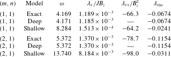
In table 2, we show that the deep-limit formulas apply very well to this cell. We focus our attention on the two waves
 $(m,n)=(1,1),(2,1)$
. Shallow-limit formulas (2.43) are also shown, only to illustrate that they are not adapted here: no existing shallow theory would be able to accurately model the metal pad roll instability in this small cell.
Variation of the relative growth rate
 $\unicode[STIX]{x1D706}_{\mathit{v}}/JB_{z}$
(a) and magnetic damping term
 $\unicode[STIX]{x1D706}_{\mathit{vv}}/B_{z}^{2}$
(b) when
 $\unicode[STIX]{x1D70E}_{1}$
is artificially increased. From
 $\unicode[STIX]{x1D70E}_{1}=250~\text{S}~\text{m}^{-1}$
to
 $\unicode[STIX]{x1D70E}_{1}=\unicode[STIX]{x1D70E}_{2}/100$
there is only a weak modification of the growth rate and magnetic damping. At
 $\unicode[STIX]{x1D70E}_{1}=\unicode[STIX]{x1D70E}_{2}$
, the instability vanishes: a strong difference in conductivity is essential for the metal pad roll instability.

The relative magnetic damping rates
 $\unicode[STIX]{x1D706}_{\mathit{vv}}/B_{z}^{2}$
(in
 $\text{s}^{-1}~\text{T}^{-2}$
) are calculated numerically for different waves
 $(m,n)$
using a finite-difference solver with variable spatial resolution
 $M=100$
, 200, 400, 800 and compared to the theoretical estimate (2.64) obtained by assuming
 $\unicode[STIX]{x1D70E}_{1}\ll \unicode[STIX]{x1D70E}_{2}$
. The numerical values converge towards the theoretical estimate.

In table 3 we compare the theoretical estimation of
 $\unicode[STIX]{x1D706}_{\mathit{vv}}/B_{z}^{2}$
given by formula (2.64) to numerically calculated values, obtained using numerical quadrature and the field profiles
 $\widehat{\unicode[STIX]{x1D6F9}}_{i}^{\mathit{v}}$
that result from the finite-difference code. Increasing the spatial resolution
 $M=100$
, 200, 400, 800 in the code, we observe that the values of the damping rates converge towards the theoretical prediction of (2.64). This validates our finite difference solver, and also suggests that our theoretical formula (2.64) for the magnetic damping rate is correct.
In figure 7, we inspect how the rates
 $\unicode[STIX]{x1D706}_{\mathit{v}}/JB_{z}$
and
 $\unicode[STIX]{x1D706}_{\mathit{vv}}/B_{z}^{2}$
of the fundamental wave
 $(m,n)=(1,1)$
may vary with the electrical conductivity of the top layer. In reality, we obviously cannot choose the conductivity of the cryolite, but we want to know how important it is to use the exact value for
 $\unicode[STIX]{x1D70E}_{1}$
. We investigate the range
 $\unicode[STIX]{x1D70E}_{1}\in [250~\text{S}~\text{m}^{-1},\unicode[STIX]{x1D70E}_{2}]$
. We use the numerical approach to calculate
 $\unicode[STIX]{x1D706}_{\mathit{vv}}/B_{z}^{2}$
, since the theoretical approximation (2.64) is not valid when
 $\unicode[STIX]{x1D70E}_{1}\not \ll \unicode[STIX]{x1D70E}_{2}$
. For
 $\unicode[STIX]{x1D70E}_{1}$
in the range
 $[250~\text{S}~\text{m}^{-1},\unicode[STIX]{x1D70E}_{2}/100]$
, we observe little change in both
 $\unicode[STIX]{x1D706}_{\mathit{v}}/JB_{z}$
and
 $\unicode[STIX]{x1D706}_{\mathit{vv}}/B_{z}^{2}$
. Increasing further
 $\unicode[STIX]{x1D70E}_{1}$
does lower the growth rate
 $\unicode[STIX]{x1D706}_{\mathit{v}}$
significantly and when
 $\unicode[STIX]{x1D70E}_{1}=\unicode[STIX]{x1D70E}_{2}$
, we ultimately get
 $\unicode[STIX]{x1D706}_{\mathit{v}}=0$
. Magnetic damping only gets stronger with increasing
 $\unicode[STIX]{x1D70E}_{1}$
, since ohmic dissipation may then also occur in the top layer. We conclude here that the low conductivity of the electrolyte
 $\unicode[STIX]{x1D70E}_{1}$
can be significantly increased without quantitively modifying the instability, but that a true jump in conductivity is crucial for the metal pad roll instability.
4.2 Numerically solved problem
The numerical methods used in SFEMaNS and OpenFOAM were previously described in Guermond et al. (Reference Guermond, Laguerre, Léorat and Nore2007, Reference Guermond, Laguerre, Léorat and Nore2009), Weber et al. (Reference Weber, Galindo, Stefani, Weier and Wondrak2013, Reference Weber, Galindo, Stefani and Weier2014, Reference Weber, Beckstein, Galindo, Herreman, Nore, Stefani and Weier2017a ,Reference Weber, Beckstein, Herreman, Horstmann, Nore, Stefani and Weier b , Reference Weber, Beckstein, Galindo, Starace and Weier2018), Nore et al. (Reference Nore, Quiroz, Cappanera and Guermond2016), Ashour et al. (Reference Ashour, Kelley, Salas, Starace, Weber and Weier2018), Cappanera et al. (Reference Cappanera, Guermond, Herreman and Nore2018) and Horstmann et al. (Reference Horstmann, Weber and Weier2018). SFEMaNS (for spectral finite element code for Maxwell and Navier–Stokes equations) is a hybrid finite element–spectral solver that can handle axisymmetric fluid domains, OpenFOAM is a public library that uses a finite volume method. Both codes are used here to solve the nonlinear momentum equation and mass balance
 $$\begin{eqnarray}\left.\begin{array}{@{}c@{}}\unicode[STIX]{x1D70C}(\unicode[STIX]{x2202}_{t}\boldsymbol{U}+(\boldsymbol{U}\boldsymbol{\cdot }\unicode[STIX]{x1D735})\boldsymbol{U})=-\unicode[STIX]{x1D735}P+\unicode[STIX]{x1D735}\boldsymbol{\cdot }(\unicode[STIX]{x1D70C}\unicode[STIX]{x1D708}(\unicode[STIX]{x1D735}\boldsymbol{U}+\unicode[STIX]{x1D735}\boldsymbol{U}^{\text{T}}))+\boldsymbol{J}\times \boldsymbol{B},\\ \unicode[STIX]{x1D735}\boldsymbol{\cdot }\boldsymbol{U}=0,\end{array}\right\}\end{eqnarray}$$
in a cylindrical fluid domain. The fields
 $\boldsymbol{U}$
,
 $P$
,
 $\boldsymbol{B}$
,
 $\boldsymbol{J}=\unicode[STIX]{x1D707}_{0}^{-1}\unicode[STIX]{x1D735}\times \boldsymbol{B}$
correspond here to the total flow, pressure, magnetic induction and current density. To deal with the multi-phase character, the material parameters
 $\unicode[STIX]{x1D70C},\unicode[STIX]{x1D708}$
are considered as space- and time-dependent functions that may be reconstructed using a scalar field
 $f\in [0,1]$
that sharply varies from 0 to 1 on the interface. This function allows us to reconstruct the material parameters of the different liquid phases, e.g.
 $\unicode[STIX]{x1D70C}=\unicode[STIX]{x1D70C}_{1}f+\unicode[STIX]{x1D70C}_{2}(1-f)$
for the density in the two-phase system. By materially advecting the indicator function
 $f$
, that is, solving
 $$\begin{eqnarray}\unicode[STIX]{x2202}_{t}f+(\boldsymbol{U}\boldsymbol{\cdot }\unicode[STIX]{x1D735})f\approx 0,\end{eqnarray}$$
we keep track of the different phases as time evolves. This is done in SFEMaNS by using a level set method. OpenFOAM uses a volume of fluid method. Surface tension may be dealt with in both codes, but SFEMaNS nor OpenFOAM use particular numerical models for the contact line motion. As a result no realistic contact angle other than
 $90^{\circ }$
can be used. Therefore, we limit all the direct numerical simulations to the case without surface tension:
 $\unicode[STIX]{x1D6FE}_{1|2}=0$
. On the side wall and top and bottom surfaces, we impose the no-slip condition.
 $$\begin{eqnarray}\boldsymbol{U}=\mathbf{0}|_{\unicode[STIX]{x1D6F4}_{1}\cup \unicode[STIX]{x1D6F4}_{2}}.\end{eqnarray}$$
This no-slip condition is imposed in a weak way and, as a result, the ‘contact line’ (region where
 $f$
changes from 0 to 1 near
 $r=R$
) can still freely slide on the cylindrical wall. The magnetic problem is solved differently in both codes. SFEMaNS solves the full induction equation and Gauss’ law
 $$\begin{eqnarray}\left.\begin{array}{@{}c@{}}\unicode[STIX]{x2202}_{t}\boldsymbol{B}=\unicode[STIX]{x1D735}\times (\boldsymbol{U}\times \boldsymbol{B})-\unicode[STIX]{x1D735}\times (\unicode[STIX]{x1D70E}^{-1}\unicode[STIX]{x1D735}\times (\unicode[STIX]{x1D707}_{0}^{-1}\boldsymbol{B})),\\ 0=\unicode[STIX]{x1D735}\boldsymbol{\cdot }\boldsymbol{B},\end{array}\right\}\end{eqnarray}$$
together with the boundary conditions
 $$\begin{eqnarray}\displaystyle B_{z}|_{r=R} & = & \displaystyle B_{z},\quad B_{\unicode[STIX]{x1D703}}|_{r=R}=\frac{\unicode[STIX]{x1D707}_{0}JR}{2},\end{eqnarray}$$
 $$\begin{eqnarray}\displaystyle \text{J}_{r}|_{z=H_{1}} & = & \displaystyle 0,\quad \text{J}_{\unicode[STIX]{x1D703}}|_{z=H_{1}}=0,\end{eqnarray}$$
 $$\begin{eqnarray}\displaystyle B_{r}|_{z=-H_{2}} & = & \displaystyle 0,\quad B_{\unicode[STIX]{x1D703}}|_{z=-H_{2}}=\frac{\unicode[STIX]{x1D707}_{0}Jr}{2},\end{eqnarray}$$
 $\unicode[STIX]{x1D70E}^{-1}$
is reconstructed using the indicator field
 $f$
. In OpenFOAM, a quasi-static MHD approach is used. The electrical field is approximated as
 $\boldsymbol{E}\approx -\unicode[STIX]{x1D735}\unicode[STIX]{x1D6F7}$
and Ohm’s law as
 $$\begin{eqnarray}\boldsymbol{J}\approx \unicode[STIX]{x1D70E}\left(-\unicode[STIX]{x1D735}\unicode[STIX]{x1D6F7}+\boldsymbol{U}\times \left(\frac{\unicode[STIX]{x1D707}_{0}Jr}{2}\boldsymbol{e}_{\unicode[STIX]{x1D703}}+B_{z}\boldsymbol{e}_{z}\right)\right).\end{eqnarray}$$
Combining this with
 $\unicode[STIX]{x1D735}\boldsymbol{\cdot }\boldsymbol{J}=0$
, we find a Poisson problem for the total electrical potential
 $\unicode[STIX]{x1D6F7}$
, that can be solved with the boundary conditions
 $$\begin{eqnarray}\text{J}_{r}=0|_{r=R},\quad \unicode[STIX]{x1D6F7}|_{z=H_{1}}=0,\quad \text{J}_{z}|_{z=-H_{2}}=J.\end{eqnarray}$$
Once the current density is known, the total magnetic field
 $\boldsymbol{B}$
can be calculated using the Biot–Savart integral. In this
 $\boldsymbol{B}$
, the base state magnetic field
 $(\unicode[STIX]{x1D707}_{0}Jr/2)\boldsymbol{e}_{\unicode[STIX]{x1D703}}+B_{z}\boldsymbol{e}_{z}$
always dominates in the quasi-static limit, but the small deviations in the magnetic field still need to be calculated in order to have a consistent approximation of the Lorentz force
 $\boldsymbol{J}\times \boldsymbol{B}$
(this correction was crucial for the Tayler instability (Weber et al.
Reference Weber, Galindo, Stefani, Weier and Wondrak2013, Reference Weber, Galindo, Stefani and Weier2014) but is likely less important here).
In both codes, we have varied the grid size to assess the numerical convergence. We introduce the non-dimensional measure
 $h=\unicode[STIX]{x1D6FF}x/R$
to characterize the grid size. In SFEMaNS the mesh size
 $\unicode[STIX]{x1D6FF}x$
is non-uniform in the plane
 $(r,z)$
and the mesh cells are refined near the interface. Therefore we provide intervals
 $h=(h_{min}\rightarrow h_{max})$
to characterize the SFEMaNS grid. All the simulations reported in the paper have been done with 30 real Fourier modes in the azimuthal direction. In SFEMaNS, we relax the conductivity jump by taking
 $\unicode[STIX]{x1D70E}_{1}=\unicode[STIX]{x1D70E}_{2}/100$
. This stabilizes the numerical calculations and, as explained above, should not modify the linear instability mechanism. In OpenFOAM only purely orthogonal cells are used with
 $h=0.05$
or smaller. The cells are flattened towards the interface with an aspect ratio of 5 at most. Interface compression ensures that the interface is typically smeared over 2–3 cells. Information on the initialization of both codes is provided below.
Using both SFEMaNS and OpenFOAM, we simulate the decay of large-scale gravity waves
 $(m,n)=(1,1),(2,1)$
with or without an imposed magnetic field
 $B_{z}=0$
, 10, 25, 50 mT and using different grids with typical mesh sizes
 $h=\unicode[STIX]{x1D6FF}x/R$
. We measure the frequency
 $\unicode[STIX]{x1D714}+\unicode[STIX]{x1D6FF}_{\mathit{visc}}$
(
 $\text{s}^{-1}$
), the viscous damping rate
 $\unicode[STIX]{x1D706}_{\mathit{visc}}$
(
 $\text{s}^{-1}$
) and the magnetic damping rates
 $\unicode[STIX]{x1D706}_{\mathit{vv}}$
(
 $\text{s}^{-1}$
) of the waves and we compare with the theoretical estimates provided by the perturbative analysis.
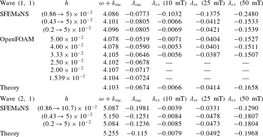
4.3 Numerical results and comparison with theory
4.3.1 Viscously damped gravity waves
In a first series of tests, we set
 $J=0$
,
 $B_{z}=0$
, initialize the numerical simulations with low amplitude gravity wave profiles for
 $(m,n)=(1,1),(2,1)$
and let these waves decay in time. We measure numerical values for the frequency and viscous damping rates of these waves and compare these measures with the viscously corrected frequency
 $\unicode[STIX]{x1D714}+\unicode[STIX]{x1D6FF}_{\mathit{visc}}$
and damping rate
 $\unicode[STIX]{x1D706}_{\mathit{visc}}$
of the theoretical model. All the results are gathered in table 4. Both solvers OpenFOAM and SFEMaNS clearly show convergence on the gravity wave frequency
 $\unicode[STIX]{x1D714}+\unicode[STIX]{x1D6FF}_{\mathit{visc}}$
as the grid is refined, and the measured frequencies closely match the theoretical value. For the fundamental wave
 $(1,1)$
, the absolute error between the theory and the numerical values is of order
 $0.01~\text{s}^{-1}$
on the finest grid, and the relative errors is of the order of
 $2.4\times 10^{-3}$
. For the wave
 $(m,n)=(2,1)$
there is a larger mismatch but the agreement is still very good. For the viscous damping rates
 $\unicode[STIX]{x1D706}_{\mathit{visc}}$
, we also observe convergence in both codes as the grid is refined. The waves are slightly more damped in the numerical simulations than predicted by the theory and there is a noticeable difference between both codes: the same waves are more viscously damped in SFEMaNS than in OpenFOAM.
4.3.2 Viscous and magnetically damped gravity waves
In a second series of tests, we measure the damping rates of gravity waves in the presence of non-zero external magnetic fields
 $B_{z}\neq 0$
, but without an electrolysis current (
 $J=0$
). We perform simulations for increasing magnetic field
 $B_{z}=10$
, 25, 50 mT. Denoting by
 $\unicode[STIX]{x1D706}$
the growth rate of the waves in the numerical simulations using a mesh with cell size
 $h$
and
 $\unicode[STIX]{x1D706}_{\mathit{visc}}$
the viscous growth rate measured for this mesh, we then calculate the numerical values
 $\unicode[STIX]{x1D706}_{\mathit{vv}}=\unicode[STIX]{x1D706}-\unicode[STIX]{x1D706}_{\mathit{visc}}$
in order to filter the code- and grid-dependent viscous damping that was considered in the previous section. Table 4 gathers the numerical measures for
 $\unicode[STIX]{x1D706}_{\mathit{vv}}$
. These measures are compared with the theoretical estimates for waves
 $(1,1)$
and
 $(2,1)$
. The agreement with the theoretical value is very good on sufficiently fine grids and excellent for the small values of
 $B_{z}=10$
, 25 mT. For the largest value
 $B_{z}=50~\text{mT}$
there is a small mismatch, which we suspect is due to the fact that we leave the asymptotic regime of validity of the theoretical model. We notice that the magnetic damping rates
 $-\unicode[STIX]{x1D706}_{\mathit{vv}}$
are slightly lower in OpenFOAM than in the simulations done with SFEMaNS.
Visualization of the interface between the cryolite and the aluminium in the numerical simulations. (a,b) Eight snapshots over one period
 $T$
in the saturated regime for
 $J=-7795~\text{A}~\text{m}^{-2}$
,
 $B_{z}=16~\text{mT}$
. (c) Far from the stability threshold, the interface violently destabilizes and develops large deformations,
 $J=-20\,000~\text{A}~\text{m}^{-2}$
,
 $B_{z}=16~\text{mT}$
.

(a) Comparison of theoretical and numerical growth rates for the large-scale sloshing wave
 $(m,n)=(1,1)$
as a function of
 $|J|$
. (b) Saturation amplitudes of rotating wave as a function of
 $|J|$
. Small cell configuration with
 $B_{z}=16~\text{mT}$
and ignoring surface tension.

4.3.3 Metal pad roll instability
In a third series of tests, we perform simulations of the metal pad roll instability with both
 $J$
and
 $B_{z}$
active. We fix the magnetic field strength to
 $B_{z}=16~\text{mT}$
which is used in Steiner (Reference Steiner2009). We increase the current density in the interval
 $J\in -[7795,25\,984]~\text{A}~\text{m}^{-2}$
which corresponds to electrolysis currents in the range
 $I=[30,100]~\text{A}$
. The current runs downwards through the cell. From the theory, we estimate that the metal pad roll instability should occur when
 $|J|$
is above the threshold
 $\text{J}_{c}=4430~\text{A}~\text{m}^{-2}$
.
Figure 8 shows snapshots from simulations at
 $|J|=7795~\text{A}~\text{m}^{-2}>\text{J}_{c}$
. The metal pad roll instability is clearly visible. We observe a saturated wave similar in shape to the fundamental wave
 $(m,n)=(1,1)$
, and this wave rotates in the anti-clockwise direction
 $(m\unicode[STIX]{x1D714}<0)$
when seen from above. This behaviour corresponds to what we expect from the theory. In a more systematic series of computations we have measured the growth rate of the metal pad roll instability as a function of
 $J$
. The results are shown in figure 9(a). We observe an excellent agreement with theory. The fact that both SFEMaNS and OpenFOAM find straight lines with the same slope is an indication that both codes capture the destabilizing mechanism at the origin of
 $\unicode[STIX]{x1D706}_{\mathit{v}}$
very well. The growth rates from SFEMaNS are slightly beneath those from OpenFOAM, which is not unexpected owing to the small difference in viscous and magnetic damping rates we have observed before.
The numerical simulations further provide insights in the nonlinear regime, but since this regime is not modelled by the proposed theory we will not study it in detail here. In figure 9(b), we show a diagram that gathers the maximal amplitude
 $\unicode[STIX]{x1D702}_{max}$
of the saturated rotating gravity wave as a function of current density. This curve suggests a supercritical bifurcation. We propose a weakly nonlinear fit
 $\unicode[STIX]{x1D702}_{max}\approx 1.5\times 10^{-4}\sqrt{|J|-\text{J}_{c}}$
in MKS units (based on the OpenFOAM data). In non-dimensional form and using the theoretical formula for the growth rate
 $\unicode[STIX]{x1D706}$
, we rewrite this fit as follows:
 $$\begin{eqnarray}\text{If }\unicode[STIX]{x1D706}>0:\quad \frac{\unicode[STIX]{x1D702}_{max}}{R}\approx 2\sqrt{\frac{\unicode[STIX]{x1D706}}{|\unicode[STIX]{x1D714}|}}.\end{eqnarray}$$
It is likely that this non-dimensional relation is more generally applicable to estimate the weakly nonlinear saturation amplitude of the fundamental wave
 $(1,1)$
in deep reduction cells, but we certainly do not expect it to be valid for shallow cells.
The weakly nonlinear regime exists only in a small parameter range. Above
 $|J|\sim 15\,000~\text{A}~\text{m}^{-2}$
, violent secondary instabilities are observed with both numerical solvers. The interface undergoes strong deformations which ultimately lead to a blow up of the numerical calculations. To illustrate this phenomenon, we show in figure 8(c) the interface obtained with
 $J=-20\,000~\text{A}~\text{m}^{-2}$
using SFEMaNS, right before the blow-up. The precise origin of this secondary instability is unknown, but in this strongly nonlinear regime we do find the ‘explosive’ combination of
 $$\begin{eqnarray}\Vert \boldsymbol{J}_{NL}-J\boldsymbol{e}_{z}\Vert \sim 1,\quad \frac{|JB_{z}|}{(\unicode[STIX]{x1D70C}_{2}-\unicode[STIX]{x1D70C}_{1})g}\geqslant 1.\end{eqnarray}$$
The total electrical current density (
 $\boldsymbol{J}_{NL}$
) may significantly differ from the equilibrium state and it is quite likely that the resulting Lorentz force can then no longer be equilibrated by pressure forces alone. If this local Lorentz force may, in addition, strongly overpower gravitational restoring forces, there is little reason for the cell to remain in a stably stratified state. Note that similar explosive behaviour was also observed in a liquid metal battery geometry (Weber et al.
Reference Weber, Beckstein, Galindo, Herreman, Nore, Stefani and Weier2017a
,Reference Weber, Beckstein, Herreman, Horstmann, Nore, Stefani and Weier
b
).
5 Application to large cells and liquid metal batteries
We further apply our theoretical model to make some linear stability predictions for large-scale, shallow reduction cells and also for a particular type of liquid metal batteries with strongly decoupled interfaces.
5.1 Large, industrial-scale cells
Industrial reduction cells are very large in lateral extent and each fluid layer is extremely shallow. As such, they are very different from the small reduction cell studied in the previous section (see the to-scale sketch of figure 10). We inspect how our theory behaves in these more realistic conditions and consider large cells, with dimensions
 $$\begin{eqnarray}R\in [0.5,5]~\text{m},\quad H_{1}=0.05~\text{m},\quad H_{2}=0.30~\text{m}.\end{eqnarray}$$
All the material parameters are taken the same as in (4.2). We ignore surface tension since the focus will be on long-wavelength waves.
To-scale side view of the two reduction cell configurations studied in the article. (a) Small experimental cell with radius
 $R=0.035~\text{m}$
used for the validation of the theory. (b) Large industrial-scale cell (in this plot
 $R=1~\text{m}$
).

Theoretical values for all the relevant quantities characterizing the stability and frequency of various waves
 $(m,n)$
in the large cell with radius
 $R=1~\text{m}$
. Interfacial tension is ignored,
 $\unicode[STIX]{x1D6FE}_{1|2}=0$
. Units are in the MKS system.
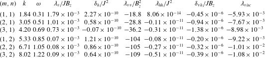
In table 5 we give the numerical values for all the relevant theoretical quantities determining the stability and frequency shifts for different waves
 $(m,n)$
in a cell of radius
 $R=1~\text{m}$
. In the column for
 $\unicode[STIX]{x1D706}_{\mathit{v}}/JB_{z}$
, we see that the fundamental wave
 $(1,1)$
is always the most unstable. Since the viscous dissipation is also the lowest for this wave, we expect this mode to be dominant in an unstable cell. The relative frequency shift
 $\unicode[STIX]{x1D6FF}_{\mathit{h}}/J^{2}$
can be either positive or negative and it decays as
 $m$
or
 $n$
increases. Although the numbers are small, this effect is no longer negligible for current densities of the order
 $J\sim 10^{4}~\text{A}~\text{m}^{-2}$
. A noteworthy detail is the positive value of
 $\unicode[STIX]{x1D706}_{\mathit{hh}}/J^{2}=8.06\times 10^{-14}~\text{s}^{-1}~\text{m}^{2}~\text{A}^{-2}$
for the wave
 $(1,1)$
: for large enough
 $J$
, this wave may be unstable even without an external magnetic field
 $B_{z}=0$
. However, it seems that this possibility is anecdotal: electrical currents would need to be so large that
 $\unicode[STIX]{x1D6FF}_{\mathit{h}}/\unicode[STIX]{x1D714}\gg 1$
so that our perturbation method would no longer be trustworthy. In table 6, we show that the shallow-limit formulas (see equations (2.43), (2.44), (2.65), (2.67)) apply very well to this shallow cell. Deep-limit formulas are not shown here but are not adapted.
Growth rate
 $\unicode[STIX]{x1D706}$
and shifted frequency
 $\unicode[STIX]{x1D714}+\unicode[STIX]{x1D6FF}$
for various gravity waves
 $(m,n)$
in large cells with dimensions
 $R\in [0.5,2.5]~\text{m}$
,
 $H_{1}=0.05~\text{m}$
,
 $H_{2}=0.35~\text{m}$
. We take realistic values for the current density
 $J=1.5\times 10^{4}~\text{A}~\text{m}^{-2}$
and the vertical magnetic field
 $B_{z}=1~\text{mT}$
. The dashed lines in (b) correspond to the unperturbed gravity wave frequency
 $\unicode[STIX]{x1D714}$
; the solid lines correspond to
 $\unicode[STIX]{x1D714}+\unicode[STIX]{x1D6FF}$
.

Comparison of the exact theoretical formulas with shallow limits for inviscid frequencies
 $\unicode[STIX]{x1D714}$
(in
 $\text{s}^{-1}$
) and relative growth rates
 $\unicode[STIX]{x1D706}_{\mathit{v}}/JB_{z}$
(in
 $\text{s}^{-1}~\text{A}^{-1}~\text{m}^{2}~\text{T}^{-1}$
), relative magnetic damping term
 $\unicode[STIX]{x1D706}_{\mathit{vv}}/B_{z}^{2}$
(in
 $\text{s}^{-1}~\text{T}^{-2}$
), viscous damping term
 $\unicode[STIX]{x1D706}_{\mathit{visc}}$
(in
 $\text{s}^{-1}$
) and relative frequency shift
 $\unicode[STIX]{x1D6FF}_{\mathit{h}}/J^{2}$
(in
 $\text{s}^{-1}~\text{A}^{-2}~\text{m}^{4}$
). In the large cell under study, the shallow-limit formulas provide a very accurate description.

We now fix
 $J=1.5\times 10^{4}~\text{A}~\text{m}^{-2}$
and
 $B_{z}=1~\text{mT}$
, which we consider to be realistic values. Due to the low strength of the magnetic field, we can just neglect all the quasi-static MHD effects in the large cell as is done usually in the metal pad roll theory for shallow cells. The following approximation applies well:
 $$\begin{eqnarray}\unicode[STIX]{x1D706}\approx \unicode[STIX]{x1D706}_{\mathit{v}}+\unicode[STIX]{x1D706}_{\mathit{visc}},\quad \unicode[STIX]{x1D6FF}\approx \unicode[STIX]{x1D6FF}_{\mathit{h}}+\unicode[STIX]{x1D6FF}_{\mathit{visc}}.\end{eqnarray}$$
In figure 11(a) we show how the theoretical growth rate
 $\unicode[STIX]{x1D706}$
increases almost linearly with
 $R$
in agreement with what was indicated by the shallow-limit formula (2.45). The large-scale sloshing mode
 $(1,1)$
is the most unstable mode over the entire
 $R$
-span and should be the selected mode in this cell. In figure 11(b), the dashed lines show the inviscid frequency
 $\unicode[STIX]{x1D714}$
and need to be compared with the solid lines that show the shifted frequency,
 $\unicode[STIX]{x1D714}+\unicode[STIX]{x1D6FF}$
. The frequency shift is clearly visible and mostly due to the contribution
 $\unicode[STIX]{x1D6FF}_{\mathit{h}}$
, i.e. it is caused by the Lorentz force interaction of the electrical currents
 $\widehat{\boldsymbol{j}}_{i}$
with the horizontal magnetic field
 $\unicode[STIX]{x1D707}_{0}Jr/2\,\boldsymbol{e}_{\unicode[STIX]{x1D703}}$
.
Large cell geometry
 $R=1~\text{m}$
. (a) Streamlines of the current perturbation
 $\widehat{\boldsymbol{j}}_{i}$
for a downward base state electrolysis current density
 $\boldsymbol{J}$
. The interface deformation is suggested by the thicker black line. (b) Normalized power density for the fundamental wave
 $(1,1)$
.

In figure 12, we show the current perturbation
 $\widehat{\boldsymbol{j}}_{i}$
together with the power density in the integrand of
 ${\mathcal{P}}_{\mathit{v}}$
. Comparison with figure 6 allows us to highlight some crucial differences between deep and shallow cells. In the shallow cell,
 $\widehat{\boldsymbol{j}}_{i}$
is mainly vertical in the electrolyte and horizontal in the aluminium. The very low
 ${\mathcal{P}}_{\mathit{v}}$
-power density in the electrolyte layer indicates that no significant mechanical power transfer occurs in the thin electrolyte layer. This is all well known for shallow cells but noticeably different from what we had in the small (deep) cell of figure 6 (symmetrical
 $\widehat{\boldsymbol{j}}_{i}$
, mechanical power transfer in both the cryolite and the aluminium).
A common statement in metal pad roll theory is that cylindrical cells are always unstable, often expressed in terms of the critical
 $\unicode[STIX]{x1D6FD}$
number as
 $\unicode[STIX]{x1D6FD}_{c}=0$
(
 $\unicode[STIX]{x1D6FD}$
defined in (1.1)). This statement obviously only holds when all dissipation is ignored, which is not the case in our theory. Focussing on large shallow cells, ignoring surface tension and magnetic damping (small), we can rearrange the equation
 $\unicode[STIX]{x1D706}_{\mathit{v},shallow}+\unicode[STIX]{x1D706}_{\mathit{visc},shallow}\approx 0$
for the onset of instability into an equation for the critical
 $\unicode[STIX]{x1D6FD}$
number in the presence of viscous damping,
 $$\begin{eqnarray}\displaystyle \unicode[STIX]{x1D6FD}_{c,mn} & {\approx} & \displaystyle \frac{\unicode[STIX]{x03C0}}{2\sqrt{2}}\frac{\unicode[STIX]{x1D705}_{mn}^{3/2}(\unicode[STIX]{x1D705}_{mn}^{2}-m^{2})}{m}\nonumber\\ \displaystyle & & \displaystyle \times \,\frac{H_{1}^{-2}\left(2+{\displaystyle \frac{\unicode[STIX]{x1D70C}_{1}\sqrt{\unicode[STIX]{x1D708}_{1}}}{\unicode[STIX]{x1D70C}_{2}\sqrt{\unicode[STIX]{x1D708}_{2}}}}\right)+2(H_{1}H_{2})^{-1}+H_{2}^{-2}\left(2+{\displaystyle \frac{\unicode[STIX]{x1D70C}_{2}\sqrt{\unicode[STIX]{x1D708}_{2}}}{\unicode[STIX]{x1D70C}_{1}\sqrt{\unicode[STIX]{x1D708}_{1}}}}\right)}{((\unicode[STIX]{x1D70C}_{2}-\unicode[STIX]{x1D70C}_{1})g)^{1/4}(\unicode[STIX]{x1D70C}_{1}H_{1}^{-1}+\unicode[STIX]{x1D70C}_{2}H_{2}^{-1})^{3/4}\left({\displaystyle \frac{1}{\unicode[STIX]{x1D70C}_{1}\sqrt{\unicode[STIX]{x1D708}_{1}}}}+{\displaystyle \frac{1}{\unicode[STIX]{x1D70C}_{2}\sqrt{\unicode[STIX]{x1D708}_{2}}}}\right)}R^{1/2}.\end{eqnarray}$$
This notation is to be interpreted as follows: when
 $\unicode[STIX]{x1D6FD}>\unicode[STIX]{x1D6FD}_{c,mn}$
the wave
 $(m,n)$
is destabilized. It is evident from this formula that the critical
 $\unicode[STIX]{x1D6FD}$
numbers increase with radius
 $R$
, which is further visualized in figure 13. This figure also shows that we can define the critical
 $\unicode[STIX]{x1D6FD}$
number as
 $\unicode[STIX]{x1D6FD}_{c}=\min _{mn}(\unicode[STIX]{x1D6FD}_{c,mn})=\unicode[STIX]{x1D6FD}_{c,11}$
since the fundamental wave
 $(1,1)$
always is the first to be destabilized. With the present geometrical choices and material parameters, we calculate
 $\unicode[STIX]{x1D6FD}_{c}\in [0.33,1.06]$
for
 $R\in [0.5,5]~\text{m}$
. The values found here for
 $\unicode[STIX]{x1D6FD}_{c}$
are not so small and so it is best that we check if these high values of
 $\unicode[STIX]{x1D6FD}$
still remain accessible to our perturbation theory. Using (2.46) with
 $m=1$
,
 $\unicode[STIX]{x1D705}_{11}\approx 1.84$
, we find
 $\unicode[STIX]{x1D706}_{\mathit{v}}/\unicode[STIX]{x1D714}=0.0394\unicode[STIX]{x1D6FD}$
. Even with
 $\unicode[STIX]{x1D6FD}\sim 1$
, the necessary condition
 $\unicode[STIX]{x1D706}_{\mathit{v}}/\unicode[STIX]{x1D714}\ll 1$
remains fulfilled so we are confident about our prediction of
 $\unicode[STIX]{x1D6FD}_{c}$
.
In the presence of viscous damping, the critical
 $\unicode[STIX]{x1D6FD}$
-number for the onset of metal pad roll instability is non-zero. Using realistic material properties and fluid layer heights, we show here how critical
 $\unicode[STIX]{x1D6FD}$
numbers
 $\unicode[STIX]{x1D6FD}_{c,mn}$
for the destabilization of different waves
 $(m,n)$
, vary with radius
 $R$
.

The formula for
 $\unicode[STIX]{x1D6FD}_{c}$
and figure 13 give the impression that larger cells are more stable, but this is without taking into account the fact that the total current
 $I$
appearing in
 $\unicode[STIX]{x1D6FD}$
can still depend on
 $R$
. In electrolysis cells, just as in liquid metal batteries, it is likely that an upper bound exists for the current density
 $J$
which is of the order
 $10^{4}~\text{A}~\text{m}^{-2}$
. Replacing
 $I=J\unicode[STIX]{x03C0}R^{2}$
in the definition (1.1) of
 $\unicode[STIX]{x1D6FD}$
, we can then rewrite the condition
 $\unicode[STIX]{x1D6FD}>\unicode[STIX]{x1D6FD}_{c}$
for the onset of instability as a more practical condition on the radius of a cylindrical cell:
 $R>R_{c}$
. Using the material properties and the typical layer heights of our modelled reduction cell,
 $J=1.5\times 10^{4}~\text{A}~\text{m}^{-2}$
and
 $B_{z}=1~\text{mT}$
, we find
 $R_{c}=0.37~\text{m}$
. This is below the dimensions of actual reduction cells, but it is not so small either: viscosity would be rather efficient in keeping moderate-scale reduction cells stable.
5.2 Mg–Sb liquid metal battery
The references Weber et al. (Reference Weber, Beckstein, Galindo, Herreman, Nore, Stefani and Weier2017a
,Reference Weber, Beckstein, Herreman, Horstmann, Nore, Stefani and Weier
b
) numerically investigate the metal pad roll instability in a
 $\text{Mg}|\text{NaCl}-\text{KCl}-\text{MgCl}_{2}|\text{Sb}$
liquid metal battery (LMB) of cylindrical shape. These batteries are structurally similar to reduction cells, except that they are composed of three layers of conducting fluid (top, middle, bottom
 $=$
indices 1, 2, 3) instead of two. The cell studied in the above references has dimensions
 $$\begin{eqnarray}R=0.05~\text{m},\quad (H_{1},H_{2},H_{3})=(0.045,0.01,0.045)~\text{m}.\end{eqnarray}$$
The material properties are
 $$\begin{eqnarray}\left.\begin{array}{@{}c@{}}(\unicode[STIX]{x1D70C}_{1},\unicode[STIX]{x1D70C}_{2},\unicode[STIX]{x1D70C}_{3})=(1577,1715,6270)~\text{kg}~\text{m}^{-3},\\ (\unicode[STIX]{x1D70E}_{1},\unicode[STIX]{x1D70E}_{2},\unicode[STIX]{x1D70E}_{3})=(3.6\times 10^{6},80,8.7\times 10^{5})~\text{S}~\text{m}^{-1},\\ (\unicode[STIX]{x1D708}_{1},\unicode[STIX]{x1D708}_{2},\unicode[STIX]{x1D708}_{3})=(6.7,6.8,2.0)\times 10^{-7}~\text{m}^{2}~\text{s}^{-1},\end{array}\right\}\end{eqnarray}$$
with the surface tensions
 $$\begin{eqnarray}(\unicode[STIX]{x1D6FE}_{1|2},\unicode[STIX]{x1D6FE}_{2|3})=(0.19,0.095)~\text{N}~\text{m}^{-1}.\end{eqnarray}$$
The top (Mg) and bottom (Sb) layers are very good conductors, but the middle layer, composed of molten salt
 $(\text{NaCl}-\text{KCl}-\text{MgCl}_{2})$
, is a badly conducting electrolyte. The numerical simulations performed in Weber et al. (Reference Weber, Beckstein, Galindo, Herreman, Nore, Stefani and Weier2017a
) are done with
 $B_{z}=10~\text{mT}$
and varying electrical currents
 $I=J\unicode[STIX]{x03C0}R^{2}$
. The metal pad roll instability is observed and growth rates are reported therein. Due to the large density ratio between the second and third layers, the instability mainly deforms the upper interface, separating the first and the second layers. This phenomenon is visible in figure 14(a), showing a snapshot of a saturated rotating wave. The lower interface only slightly deforms and the whole bottom layer does not really participate in the dynamics. Actually, closer inspection reveals that the frequency of the wave matches very closely that of the two-layer system composed of the first and the second layer. This observation has motivated us to try to apply our two-layer reduction cell theory to this three-layer LMB.
The following ‘technical’ operations are necessary in order to apply the theory. We entirely ignore region 3 and all that may occur there. At the interface of regions 2 and 3, the electrical boundary condition, as seen from the electrolyte is very similar to the one we had on the top cap of our cylindrical Hall–Héroult cell: the electrolyte meets there a much better conductor which we henceforth assume to be perfect. This means that if we exchange regions 1 and 2 and invert the sense of gravity i.e.
 $g\rightarrow -g$
, the theory and the formulas developed in the previous sections apply. The only difference is that the sense of rotation of the unstable wave has to be inverted. Finally, all the horizontal field effects are negligible here, just as in the small reduction cell model.
(a) Snapshot of a numerical simulation of the metal pad roll instability in a Mg–Sb liquid metal battery.
 $J=10^{4}~\text{A}~\text{m}^{-2}$
,
 $B_{z}=10~\text{mT}$
. (b) Growth rate of the metal pad roll instability in the numerical simulations and according to our two-layer theory.

In figure 14, we compare the theoretical growth rates with simulations done with OpenFOAM for various values of the current. The dashed line corresponds to our theoretical estimate
 $\unicode[STIX]{x1D706}=\unicode[STIX]{x1D706}_{\mathit{v}}+\unicode[STIX]{x1D706}_{\mathit{vv}}+\unicode[STIX]{x1D706}_{\mathit{visc}}$
. The data points are those from figure 9 in Weber et al. (Reference Weber, Beckstein, Galindo, Herreman, Nore, Stefani and Weier2017a
). The agreement is surprisingly good. The fact that we find the right slope with our two-layer theory implies that
 $\unicode[STIX]{x1D706}_{\mathit{v}}$
is correctly calculated. The threshold also seems approximatively right, which suggests that the combined magnetic and viscous damping rates
 $\unicode[STIX]{x1D706}_{\mathit{vv}}+\unicode[STIX]{x1D706}_{\mathit{visc}}$
are also more or less correct.
Since our model does quite a decent job in predicting the onset of instability, we want to use it to make some estimates for a much larger, more realistic battery system. We imagine a cell with shallow layers, keeping, for simplicity, the same fluid heights
 $H_{i}$
and material properties
 $\unicode[STIX]{x1D70C}_{i},\unicode[STIX]{x1D70E}_{i},\unicode[STIX]{x1D708}_{i}$
as in the cell of Weber et al. (Reference Weber, Beckstein, Galindo, Herreman, Nore, Stefani and Weier2017a
,Reference Weber, Beckstein, Herreman, Horstmann, Nore, Stefani and Weier
b
) but greatly increasing its radius
 $R$
. We limit the current density to the realistic value of (i)
 $J=3~\text{k}\text{A}\text{m}^{-2}$
for Mg–Sb cells or to a more optimistic one (ii)
 $J=10~\text{k}\text{A}\text{m}^{-2}$
(both scenarios were also considered in Herreman et al. (Reference Herreman, Nore, Cappanera and Guermond2015)). We also suppose a weak external magnetic field
 $B_{z}\approx 1~\text{mT}$
that is more realistic. Using the formula (5.3) (invert
 $1\leftrightarrow 2$
and change
 $g\rightarrow -g$
) we find the critical
 $\unicode[STIX]{x1D6FD}$
number
 $$\begin{eqnarray}\unicode[STIX]{x1D6FD}_{c}\approx 2.81R^{1/2}\quad (R\text{ in units of m}),\end{eqnarray}$$
which yields
 $$\begin{eqnarray}\text{(i) }R_{c}=0.32~\text{m},\quad \text{(ii) }R_{c}=0.14~\text{m}\end{eqnarray}$$
as critical radii in the two current density scenarios. These values suggest that metal pad roll instability can indeed appear in liquid metal batteries with relatively moderate sizes, approximatively in the same range as the critical radii for the Tayler instability (Herreman et al. Reference Herreman, Nore, Cappanera and Guermond2015). A more detailed nonlinear study is required to be able to find the critical sizes at which the interface motion becomes too large and potentially is detrimental for the liquid metal battery’s integrity.
6 Conclusion
Using a regular perturbation method, we have derived analytical formulas for the destabilization, the magnetic damping and the viscous damping of gravity waves in cylindrical reduction cells with layers of arbitrary heights. From the general formulas, we have derived asymptotic expressions for the deep and the shallow limits. In appendix B, we demonstrated that the model overlaps with available metal pad roll theories in the inviscid, magneto-static and small
 $\unicode[STIX]{x1D6FD}$
-limit.
The theoretical expressions for the viscous damping rates of gravity waves in cylinders in two-fluid systems are new, and to test their validity, we have conducted some hydrodynamic experiments using the orbital sloshing device described in Horstmann et al. (Reference Horstmann, Wylega and Weier2019). The measured viscous damping rates are in excellent agreement with the theoretical formulas. Improvements of the theory are still possible by taking into account damping caused by viscous dissipation near the free interface or by using a better boundary layer model near the moving contact line (see Viola & Gallaire (Reference Viola and Gallaire2018) for example).
We have applied the theoretical model to a small reduction cell that is directly inspired by the numerical study of Flueck et al. (Reference Flueck, Hofer, Picasso, Rappaz and Steiner2009) and Steiner (Reference Steiner2009). In this small cell, we have been able to do a very critical comparison with direct numerical simulations, here done using SFEMaNS and OpenFOAM. This shows that our theory captures all the stabilizing and destabilizing effects correctly and it also validates both solvers that pass here a not so simple, physical benchmark.
We further applied the theoretical model to large industrial-scale cells. Viscous effects and quasi-static corrections always remain small in large cells, in agreement with what is frequently assumed, but this does not imply that
 $\unicode[STIX]{x1D6FD}_{c}=0$
for the metal pad roll instability. Using the viscous damping rate formula, we precisely estimate the critical threshold
 $\unicode[STIX]{x1D6FD}_{c}$
for the metal pad roll instability in shallow cylindrical cells.
Finally we also showed that the proposed model can quantitively describe the metal pad roll instability in Mg–Sb liquid metal batteries. In these three-layered cells, the bottom layer is so heavy that it does not participate actively. With some well justified minor technical modifications we have shown that the model reproduces very well the growth rates numerically obtained in Weber et al. (Reference Weber, Beckstein, Galindo, Herreman, Nore, Stefani and Weier2017a
). The theoretical model allows us to make some estimates on more realistic battery systems. Using typical values for material parameters and fluid layer heights, we estimate that the metal pad roll instability may occur in cells that have moderate sizes, say
 $R>0.32~\text{m}$
.
The present study opens a few perspectives. First of all, we think that the proposed theory can be used to benchmark multiphase MHD codes. We have found that the codes SFEMaNS and OpenFOAM yield somewhat similar results and are in agreement with the theory. We invite other groups to try to reproduce these results to test the accuracy and performance of their solvers on this small cell set-up. Second, it is possible to apply the proposed perturbation method to cells with a rectangular geometry in order to derive a theoretical model for the experiments reported in Pedchenko et al. (Reference Pedchenko, Molokov, Priede, Lukyanov and Thomas2009, Reference Pedchenko, Molokov and Bardet2017). Or alternatively, perhaps these experiments could be done in a cylindrical geometry to make comparisons with the present model. Third, we plan to extend the two-layer model to three layers of fluid to be able to model the metal pad roll instability in arbitrary liquid metal batteries. As shown by several authors (Horstmann et al. Reference Horstmann, Weber and Weier2018; Molokov Reference Molokov2018; Zikanov Reference Zikanov2018), the waves on the two interfaces may interact more or less depending on the density differences between the three layers. In the uncoupled regime the present two-layer theory should be adequate, but in the strongly coupled regime (similar density jumps on top and bottom interfaces) one must model how pairs of rotating waves interact. Finally, we also need to assess the nonlinear regime of the metal pad roll instability in more detail, preferentially in shallow cell geometries which are more challenging to direct numerical simulations.
Acknowledgements
The HPC resources for SFEMaNS were provided by GENCI-IDRIS (grant 2017-0254) in France and by the Texas A&M University Brazos HPC cluster. J.-L.G. acknowledges support from University Paris Sud, the National Science Foundation under grants DMS 1620058, DMS 1619892, the Air Force Office of Scientific Research, USAF, under grant/contract no. FA99550-12-0358 and the Army Research Office, under grant no. W911NF-15-1-0517. L.C. is thankful to Texas A&M University, LIMSI, and CNRS for their financial support. N.W. is thankful for the resources provided by the Deutsche Forschungsgemeinschaft, award no. 338560565.
Supplementary material
Supplementary material is available at https://doi.org/10.1017/jfm.2019.642.
Appendix A. Details on the analytical calculation of
$\unicode[STIX]{x1D706}_{\mathit{v}}$
and
$\unicode[STIX]{x1D6FF}_{\mathit{h}}$


We explain how the solvability condition (2.36)
 $$\begin{eqnarray}\mathop{\sum }_{i=1,2}\int _{V_{i}}[\widehat{\boldsymbol{u}}_{i}^{\ast }\boldsymbol{\cdot }(\unicode[STIX]{x1D6FC}\unicode[STIX]{x1D70C}_{i}\widehat{\boldsymbol{u}}_{i}+\text{i}\unicode[STIX]{x1D714}\unicode[STIX]{x1D70C}_{i}\widetilde{\boldsymbol{u}}_{i}+\unicode[STIX]{x1D735}\widetilde{p}_{i})+\widehat{p}_{i}^{\ast }\unicode[STIX]{x1D735}\boldsymbol{\cdot }\widetilde{\boldsymbol{u}}_{i}]\,\text{d}V=\underbrace{\mathop{\sum }_{i=1,2}\int _{V_{i}}\widehat{\boldsymbol{u}}_{i}^{\ast }\boldsymbol{\cdot }(\widehat{\boldsymbol{j}}_{i}\times \boldsymbol{B}+\boldsymbol{J}\times \widehat{\boldsymbol{b}}_{i})\,\text{d}V}_{{\mathcal{P}}},\end{eqnarray}$$
is simplified in order to find the formulas for
 $\unicode[STIX]{x1D706}_{\mathit{v}}$
and
 $\unicode[STIX]{x1D706}_{\mathit{h}}$
. We introduce the notation
 ${\mathcal{P}}$
for the ‘power’ injected by the Lorentz force. On the left-hand side, we use integration by parts to bring all the partial derivatives in space on the hatted variables. Using the leading-order balances (2.31), we then find that
 $$\begin{eqnarray}\underbrace{\unicode[STIX]{x1D6FC}\mathop{\sum }_{i=1}^{2}\int _{V_{i}}\unicode[STIX]{x1D70C}_{i}|\widehat{\boldsymbol{u}}_{i}|^{2}\,\text{d}V}_{T_{1}}+\underbrace{\mathop{\sum }_{i=1}^{2}\oint _{\unicode[STIX]{x1D6FF}V_{i}}(\widehat{p}_{i}^{\ast }\widetilde{\boldsymbol{u}}_{i}+\widetilde{p}_{i}\widehat{\boldsymbol{u}}_{i}^{\ast })\boldsymbol{\cdot }\boldsymbol{n}_{i}\,\text{d}S}_{T_{2}}={\mathcal{P}}.\end{eqnarray}$$
The first group of terms
 $T_{1}$
is proportional to kinetic energy. Using the boundary conditions for the hatted and tilded variables, we reduce the second group
 $T_{2}$
to
 $$\begin{eqnarray}\displaystyle T_{2} & = & \displaystyle \unicode[STIX]{x1D6FC}\int _{{\mathcal{S}}}(\widehat{p}_{2}^{\ast }-\widehat{p}_{1}^{\ast })|_{z=0}\widehat{\unicode[STIX]{x1D702}}\,\text{d}S=\unicode[STIX]{x1D6FC}\int _{{\mathcal{S}}}(-\unicode[STIX]{x1D6FE}_{1|2}\unicode[STIX]{x1D6FB}^{2}\widehat{\unicode[STIX]{x1D702}}^{\ast }+(\unicode[STIX]{x1D70C}_{2}-\unicode[STIX]{x1D70C}_{1})g\widehat{\unicode[STIX]{x1D702}}^{\ast })\widehat{\unicode[STIX]{x1D702}}\,\text{d}S\nonumber\\ \displaystyle & = & \displaystyle \unicode[STIX]{x1D6FC}\int _{{\mathcal{S}}}(\unicode[STIX]{x1D6FE}_{1|2}|\unicode[STIX]{x1D735}\widehat{\unicode[STIX]{x1D702}}|^{2}+(\unicode[STIX]{x1D70C}_{2}-\unicode[STIX]{x1D70C}_{1})g|\widehat{\unicode[STIX]{x1D702}}|^{2})|_{z=0}\,\text{d}S\nonumber\\ \displaystyle & = & \displaystyle \unicode[STIX]{x1D6FC}\underbrace{[(\unicode[STIX]{x1D70C}_{2}-\unicode[STIX]{x1D70C}_{1})g+\unicode[STIX]{x1D6FE}_{1|2}k^{2}]\int _{{\mathcal{S}}}|\widehat{\unicode[STIX]{x1D702}}|^{2}\,\text{d}S}_{{\mathcal{K}}}.\end{eqnarray}$$
Notice that in the integration by parts we have used the boundary condition
 $\unicode[STIX]{x2202}_{r}\widehat{\unicode[STIX]{x1D702}}|_{r=R}=0$
, which is always satisfied by the inviscid gravity waves if the contact angle is
 $90^{\circ }$
. This reformulation allows us to see that
 $T_{2}$
is proportional to the potential energy and so that
 $T_{1}+T_{2}$
is proportional to the mechanical energy. Using again integration by parts, the fact that the waves derive from harmonic potentials, see (2.11), and the hydrodynamic boundary conditions, one can further demonstrate that
 $T_{1}=T_{2}$
, for the simple harmonic wave under study,
 $$\begin{eqnarray}\displaystyle T_{1} & = & \displaystyle \unicode[STIX]{x1D6FC}\left[\unicode[STIX]{x1D70C}_{1}\oint _{\unicode[STIX]{x1D6FF}V_{1}}\widehat{\unicode[STIX]{x1D719}}_{1}^{\ast }\unicode[STIX]{x1D735}\widehat{\unicode[STIX]{x1D719}}_{1}\boldsymbol{\cdot }\boldsymbol{n}_{1}\,\text{d}S+\unicode[STIX]{x1D70C}_{2}\oint _{\unicode[STIX]{x1D6FF}V_{2}}\widehat{\unicode[STIX]{x1D719}}_{2}^{\ast }\unicode[STIX]{x1D735}\widehat{\unicode[STIX]{x1D719}}_{2}\boldsymbol{\cdot }\boldsymbol{n}_{2}\,\text{d}S\right]\nonumber\\ \displaystyle & = & \displaystyle \unicode[STIX]{x1D6FC}\int _{{\mathcal{S}}}(-\text{i}\unicode[STIX]{x1D70C}_{1}\unicode[STIX]{x1D714}\widehat{\unicode[STIX]{x1D719}}_{1}^{\ast }+\text{i}\unicode[STIX]{x1D70C}_{2}\unicode[STIX]{x1D714}\widehat{\unicode[STIX]{x1D719}}_{2}^{\ast })|_{z=0}\widehat{\unicode[STIX]{x1D702}}\,\text{d}S\nonumber\\ \displaystyle & = & \displaystyle \unicode[STIX]{x1D6FC}\int _{{\mathcal{S}}}(\widehat{p}_{2}^{\ast }-\widehat{p}_{1}^{\ast })|_{z=0}\widehat{\unicode[STIX]{x1D702}}\,\text{d}S=T_{2}.\end{eqnarray}$$
The immediate consequence of this identity is that the solvability condition (2.36) reduces to
 $2\unicode[STIX]{x1D6FC}{\mathcal{K}}={\mathcal{P}}$
. Then the equation for the eigenvalue shift is
 $\unicode[STIX]{x1D6FC}={\mathcal{P}}/2{\mathcal{K}}$
. In the article, we further split
 ${\mathcal{P}}={\mathcal{P}}_{\mathit{v}}+{\mathcal{P}}_{\mathit{h}}$
with
 $$\begin{eqnarray}\displaystyle {\mathcal{P}}_{\mathit{v}} & = & \displaystyle \mathop{\sum }_{i=1,2}\int _{V_{i}}\widehat{\boldsymbol{u}}_{i}^{\ast }\boldsymbol{\cdot }(\widehat{\boldsymbol{j}}_{i}\times B_{z}\boldsymbol{e}_{z})\,\text{d}V,\end{eqnarray}$$
 $$\begin{eqnarray}\displaystyle {\mathcal{P}}_{\mathit{h}} & = & \displaystyle \mathop{\sum }_{i=1,2}\int _{V_{i}}\widehat{\boldsymbol{u}}_{i}^{\ast }\boldsymbol{\cdot }[\widehat{\boldsymbol{j}}_{i}\times (\unicode[STIX]{x1D707}_{0}Jr/2)\boldsymbol{e}_{\unicode[STIX]{x1D703}}+J\boldsymbol{e}_{z}\times \widehat{\boldsymbol{b}}_{i}]\,\text{d}V.\end{eqnarray}$$
 ${\mathcal{P}}_{\mathit{h}}$
is different from that in the article and involves the magnetic field
 $\widehat{\boldsymbol{b}}_{i}$
which is undesirable, the magnetic field is too difficult to calculate. Using the potential nature of the flow and
 $\unicode[STIX]{x1D735}\times (J\boldsymbol{e}_{z})=\mathbf{0}$
, we can transform this term as follows:
 $$\begin{eqnarray}\displaystyle \widehat{\boldsymbol{u}}_{i}^{\ast }\boldsymbol{\cdot }(J\boldsymbol{e}_{z}\times \widehat{\boldsymbol{b}}_{i})=\unicode[STIX]{x1D735}\boldsymbol{\cdot }(\widehat{\unicode[STIX]{x1D719}}_{i}^{\ast }(J\boldsymbol{e}_{z}\times \widehat{\boldsymbol{b}}_{i}))+\widehat{\unicode[STIX]{x1D719}}_{i}^{\ast }J\boldsymbol{e}_{z}\boldsymbol{\cdot }(\unicode[STIX]{x1D735}\times \widehat{\boldsymbol{b}}_{i}). & & \displaystyle\end{eqnarray}$$
Using Ampère’s law
 $\unicode[STIX]{x1D735}\times \widehat{\boldsymbol{b}}_{i}=\unicode[STIX]{x1D707}_{0}\widehat{\boldsymbol{j}}_{i}$
and after integrating over the volume this then yields
 $$\begin{eqnarray}{\mathcal{P}}_{\mathit{h}}=\mathop{\sum }_{i=1,2}\int _{V_{i}}\{\widehat{\boldsymbol{u}}_{i}^{\ast }\boldsymbol{\cdot }[\widehat{\boldsymbol{j}}_{i}\times (\unicode[STIX]{x1D707}_{0}Jr/2)\boldsymbol{e}_{\unicode[STIX]{x1D703}}]+\unicode[STIX]{x1D707}_{0}J\widehat{\unicode[STIX]{x1D719}}_{i}^{\ast }\widehat{j}_{i,z}\}\,\text{d}V+J\underbrace{\oint _{\unicode[STIX]{x1D6FF}V_{i}}\widehat{\unicode[STIX]{x1D719}}_{i}^{\ast }(\widehat{\boldsymbol{b}}_{i}\times \boldsymbol{n}_{i})\boldsymbol{\cdot }\boldsymbol{e}_{z}\,\text{d}S}_{=0}.\end{eqnarray}$$
The underbraced boundary term indeed vanishes. On the top and bottom surfaces and at the interface we have
 $\boldsymbol{n}_{i}=\pm \boldsymbol{e}_{z}$
; on the side wall we supposed that (2.8) was assumed as a boundary condition. In conclusion, with the hypothesis (2.8), we do not need to calculate the magnetic field
 $\widehat{\boldsymbol{b}}_{i}$
to get access to
 ${\mathcal{P}}_{\mathit{h}}$
and
 $\unicode[STIX]{x1D6FF}_{\mathit{h}}$
.
To calculate the integrals appearing in
 ${\mathcal{K}}$
,
 ${\mathcal{P}}_{\mathit{v}}$
analytically, we use the following formula
 $$\begin{eqnarray}\int _{0}^{R}\text{J}_{m}^{2}(kr)r\,\text{d}r=\frac{1}{2k^{2}}(k^{2}R^{2}-m^{2})\text{J}_{m}^{2}(kR),\end{eqnarray}$$
that derives from Watson (Reference Watson1995), p. 135, combined with the identity
 $\text{J}_{m}^{\prime }(kR)=0$
that applies to our gravity waves. Note here that the first formula also suggests
 $(k^{2}R^{2}-m^{2})>0$
for all of the gravity waves under study, which is a property that we have used in the paper. With the definition (A 3) for
 ${\mathcal{K}}$
and the expression for
 $\widehat{\unicode[STIX]{x1D702}}$
, we find
 $$\begin{eqnarray}{\mathcal{K}}=[(\unicode[STIX]{x1D70C}_{2}-\unicode[STIX]{x1D70C}_{1})g+\unicode[STIX]{x1D6FE}_{1|2}k^{2}]\frac{\unicode[STIX]{x03C0}|A|^{2}R^{2}}{k^{2}}(k^{2}R^{2}-m^{2})\text{J}_{m}^{2}(kR).\end{eqnarray}$$
The volume integrals in the expression (A 5a
) that defines
 ${\mathcal{P}}_{\mathit{v}}$
, are transformed into surface integrals by remarking that the two integrands can be written in conserved form:
 $\unicode[STIX]{x1D735}\widehat{\unicode[STIX]{x1D719}}_{i}^{\ast }\boldsymbol{\cdot }(-\unicode[STIX]{x1D70E}_{i}\unicode[STIX]{x1D735}\widehat{\unicode[STIX]{x1D711}}_{i}\times B_{z}\boldsymbol{e}_{z})=\unicode[STIX]{x1D735}\boldsymbol{\cdot }[-\unicode[STIX]{x1D70E}_{i}\widehat{\unicode[STIX]{x1D719}}_{i}^{\ast }\unicode[STIX]{x1D735}\widehat{\unicode[STIX]{x1D711}}_{i}\times B_{z}\boldsymbol{e}_{z}]$
. This yields
 $$\begin{eqnarray}\displaystyle {\mathcal{P}}_{\mathit{v}} & = & \displaystyle 2\unicode[STIX]{x03C0}(-\text{i}m)B_{z}\left(\unicode[STIX]{x1D70E}_{1}\int _{0}^{H_{1}}\widehat{\unicode[STIX]{x1D719}}_{1}^{\ast }\widehat{\unicode[STIX]{x1D711}}_{1}|_{r=R}\,\text{d}z+\unicode[STIX]{x1D70E}_{2}\int _{-H_{2}}^{0}\widehat{\unicode[STIX]{x1D719}}_{2}^{\ast }\widehat{\unicode[STIX]{x1D711}}_{2}|_{r=R}\,\text{d}z\right)\nonumber\\ \displaystyle & = & \displaystyle \frac{\unicode[STIX]{x03C0}mJB_{z}|A|^{2}\unicode[STIX]{x1D714}R^{2}\unicode[STIX]{x1D6EC}}{k^{2}}\left[\tanh (kH_{1})+\frac{(kH_{2})}{\sinh ^{2}(kH_{2})}+\frac{1}{\tanh (kH_{2})}\right]\text{J}_{m}^{2}(kR),\end{eqnarray}$$
with
 $\unicode[STIX]{x1D6EC}$
defined in (2.39c
). The ratio
 ${\mathcal{P}}_{\mathit{v}}/2{\mathcal{K}}$
yields the growth rate
 $\unicode[STIX]{x1D706}_{\mathit{v}}$
given in the text. The calculation of
 ${\mathcal{P}}_{\mathit{h}}$
is straightforward but lengthy and not fully presented here. A useful identity is
 $$\begin{eqnarray}\int _{0}^{R}\text{J}_{m}(kr)\unicode[STIX]{x2202}_{r}[\text{J}_{m}(kr)]r^{2}\,\text{d}r=\frac{m^{2}}{2k^{2}}\text{J}_{m}^{2}(kR).\end{eqnarray}$$
Appendix B. Linking
$\unicode[STIX]{x1D706}_{\mathit{v}}$
to existing shallow models

Both Davidson & Lindsay (Reference Davidson and Lindsay1998) and Lukyanov et al. (Reference Lukyanov, El and Molokov2001) provide shallow models for the metal pad roll instability in a cylindrical geometry in the inviscid and magnetostatic limit and without surface tension. Here we show that our expression of the growth rate (2.39) coincides with the above models when passing to the limit.
We start from the model of Lukyanov et al. (Reference Lukyanov, El and Molokov2001) and to avoid conflicts of notation, we adapt the formulas therein to our setting. The two-dimensional problem to be solved in the shallow approximation is
 $$\begin{eqnarray}\unicode[STIX]{x2202}_{tt}^{2}\unicode[STIX]{x1D702}-c^{2}\unicode[STIX]{x1D6FB}^{2}\unicode[STIX]{x1D702}=0,\quad \unicode[STIX]{x1D6FB}^{2}\unicode[STIX]{x1D712}=\overline{\unicode[STIX]{x1D6FD}}\unicode[STIX]{x1D702}.\end{eqnarray}$$
Here
 $\unicode[STIX]{x1D702}(r,\unicode[STIX]{x1D703},t)$
is the perturbation of the surface elevation, and
 $\unicode[STIX]{x1D712}(r,\unicode[STIX]{x1D703},t)$
is the perturbation on the electrical potential. The wave speed
 $c$
and the parameter
 $\overline{\unicode[STIX]{x1D6FD}}$
are defined by
 $$\begin{eqnarray}c^{2}=\frac{(\unicode[STIX]{x1D70C}_{2}-\unicode[STIX]{x1D70C}_{1})g}{\unicode[STIX]{x1D70C}_{1}H_{1}^{-1}+\unicode[STIX]{x1D70C}_{1}H_{2}^{-1}},\quad \overline{\unicode[STIX]{x1D6FD}}=\frac{JB_{z}}{(\unicode[STIX]{x1D70C}_{2}-\unicode[STIX]{x1D70C}_{1})gH_{1}H_{2}}.\end{eqnarray}$$
Note that the quantity
 $\overline{\unicode[STIX]{x1D6FD}}$
used here is not a non-dimensional number. On the right-hand side of the equation for
 $\unicode[STIX]{x1D712}$
in (B 1), we find
 $+\overline{\unicode[STIX]{x1D6FD}}\unicode[STIX]{x1D702}$
(instead of
 $-\overline{\unicode[STIX]{x1D6FD}}\unicode[STIX]{x1D702}$
in Lukyanov et al. (Reference Lukyanov, El and Molokov2001)), because in the present article we use the convention that the electrolysis current density is
 $\boldsymbol{J}=J\boldsymbol{e}_{z}$
(instead of
 $\boldsymbol{J}=-J\boldsymbol{e}_{z}$
in Lukyanov et al. (Reference Lukyanov, El and Molokov2001)). On the lateral side wall
 $r=R$
, the following conditions must be met:
 $$\begin{eqnarray}\unicode[STIX]{x2202}_{r}\unicode[STIX]{x1D712}|_{r=R}=0,\quad \unicode[STIX]{x2202}_{r}\unicode[STIX]{x1D702}|_{r=R}=-R^{-1}\unicode[STIX]{x2202}_{\unicode[STIX]{x1D703}}\unicode[STIX]{x1D712}|_{r=R}.\end{eqnarray}$$
The solutions to (B 1) take the form
 $$\begin{eqnarray}\unicode[STIX]{x1D702}=A\text{J}_{m}(kr)\,\text{e}^{\text{i}(m\unicode[STIX]{x1D703}+\unicode[STIX]{x1D714}t)},\quad \unicode[STIX]{x1D712}=(-A\overline{\unicode[STIX]{x1D6FD}}k^{-2}\text{J}_{m}(kr)+Cr^{m})\,\text{e}^{\text{i}(m\unicode[STIX]{x1D703}+\unicode[STIX]{x1D714}t)},\end{eqnarray}$$
with
 $k^{2}=\unicode[STIX]{x1D714}^{2}/c^{2}$
and
 $A$
,
 $C$
are arbitrary constants. Note that for the exponential factors we have chosen the convention
 $\exp (\text{i}(m\unicode[STIX]{x1D703}+\unicode[STIX]{x1D714}t))$
(instead of
 $\exp (\text{i}(m\unicode[STIX]{x1D703}-\unicode[STIX]{x1D714}t))$
in Lukyanov et al. (Reference Lukyanov, El and Molokov2001)). By enforcing the boundary conditions, we find the non-dimensional dispersion relation,
 $$\begin{eqnarray}\unicode[STIX]{x1D6FD}\text{J}_{m+1}(\unicode[STIX]{x1D705})=-\text{i}\unicode[STIX]{x03C0}\unicode[STIX]{x1D705}^{2}\text{J}_{m}^{\prime }(\unicode[STIX]{x1D705}),\end{eqnarray}$$
with
 $\unicode[STIX]{x1D705}=kR$
and
 $\unicode[STIX]{x1D6FD}$
as defined in (1.1). We now derive an approximate solution of (B 5) in the limit
 $\unicode[STIX]{x1D6FD}\ll 1$
. We start with the expansion
 $$\begin{eqnarray}\unicode[STIX]{x1D705}=\unicode[STIX]{x1D705}^{(0)}+\unicode[STIX]{x1D6FD}\unicode[STIX]{x1D705}^{(1)}+O(\unicode[STIX]{x1D6FD}^{2}),\end{eqnarray}$$
which we insert into (B 5). Then we expand the dispersion relation using Taylor series in powers of
 $\unicode[STIX]{x1D6FD}$
. At the order
 $O(\unicode[STIX]{x1D6FD}^{0})$
, we find the constraint
 $$\begin{eqnarray}0=-\text{i}\unicode[STIX]{x03C0}(\unicode[STIX]{x1D705}^{(0)})^{2}\text{J}_{m}^{\prime }(\unicode[STIX]{x1D705}^{(0)})\quad \Rightarrow \quad \unicode[STIX]{x1D705}^{(0)}=\unicode[STIX]{x1D705}_{mn}.\end{eqnarray}$$
Hence, for any
 $m$
the leading order of the non-dimensional radial wavenumber is the same as the one we have obtained in our model (see (2.13)). At order the
 $O(\unicode[STIX]{x1D6FD}^{1})$
, we have the constraint
 $$\begin{eqnarray}\text{J}_{m+1}(\unicode[STIX]{x1D705}_{mn})=-\text{i}\unicode[STIX]{x03C0}[\unicode[STIX]{x1D705}^{(1)}(\unicode[STIX]{x1D705}_{mn})^{2}\text{J}_{m}^{\prime \prime }(\unicode[STIX]{x1D705}_{mn})+2\unicode[STIX]{x1D705}^{(1)}\unicode[STIX]{x1D705}_{mn}\text{J}_{m}^{\prime }(\unicode[STIX]{x1D705}_{mn})].\end{eqnarray}$$
Using
 $\text{J}_{m}^{\prime }(\unicode[STIX]{x1D705}_{mn})=0$
together with the recurrence relations and the Bessel differential equation, we have
 $$\begin{eqnarray}\text{J}_{m+1}(\unicode[STIX]{x1D705}_{mn})=\frac{m}{\unicode[STIX]{x1D705}_{mn}}\text{J}_{m}(\unicode[STIX]{x1D705}_{mn}),\quad J_{m}^{\prime \prime }(\unicode[STIX]{x1D705}_{mn})=-\left(\frac{\unicode[STIX]{x1D705}_{mn}^{2}-m^{2}}{\unicode[STIX]{x1D705}_{mn}^{2}}\right)\text{J}_{m}(\unicode[STIX]{x1D705}_{mn}).\end{eqnarray}$$
This in turn yields the following simplified expression for
 $\unicode[STIX]{x1D705}^{(1)}$
:
 $$\begin{eqnarray}\text{i}\unicode[STIX]{x1D705}^{(1)}=\frac{m}{\unicode[STIX]{x03C0}\unicode[STIX]{x1D705}_{mn}(\unicode[STIX]{x1D705}_{mn}^{2}-m^{2})}.\end{eqnarray}$$
The small shift in wavenumber
 $\unicode[STIX]{x1D705}^{(1)}$
is equivalent to a small shift in the complex frequency
 $\unicode[STIX]{x1D714}$
of the waves, since by definition
 $\unicode[STIX]{x1D714}=\pm (c\unicode[STIX]{x1D705}/R)$
in the context of the shallow layer approximation. Using the expansion
 $$\begin{eqnarray}\unicode[STIX]{x1D714}=\unicode[STIX]{x1D714}^{(0)}+\unicode[STIX]{x1D6FD}\unicode[STIX]{x1D714}^{(1)}+O(\unicode[STIX]{x1D6FD}^{2}),\end{eqnarray}$$
we obtain
 $$\begin{eqnarray}\unicode[STIX]{x1D714}^{(0)}=\unicode[STIX]{x1D714}_{\mathit{shallow}}=\pm \frac{c\unicode[STIX]{x1D705}_{mn}}{R},\quad \unicode[STIX]{x1D714}^{(1)}=\pm \unicode[STIX]{x1D6FD}\frac{c\unicode[STIX]{x1D705}^{(1)}}{R}.\end{eqnarray}$$
We recognize
 $\unicode[STIX]{x1D714}^{(0)}$
as the eigenfrequency
 $\unicode[STIX]{x1D714}_{\mathit{shallow}}$
of the non-dispersive gravity waves in the shallow layer limit. The complex frequency shift
 $\unicode[STIX]{x1D6FC}$
of our model is
 $$\begin{eqnarray}\unicode[STIX]{x1D6FC}=\text{i}\unicode[STIX]{x1D714}^{(1)}=\unicode[STIX]{x1D6FD}\frac{m\unicode[STIX]{x1D714}^{(0)}}{\unicode[STIX]{x1D705}_{mn}^{2}-m^{2}}\frac{1}{\unicode[STIX]{x03C0}\unicode[STIX]{x1D705}_{mn}^{2}}.\end{eqnarray}$$
This is exactly the shallow limit of the growth rate
 $\unicode[STIX]{x1D706}_{\mathit{v}}$
with
 $\unicode[STIX]{x1D6FE}_{1|2}=0$
as stated in (2.46); recall that
 $\unicode[STIX]{x1D705}_{mn}:=kR$
. In conclusion, our results coincide with those of Davidson & Lindsay (Reference Davidson and Lindsay1998) and Lukyanov et al. (Reference Lukyanov, El and Molokov2001) in the inviscid, magnetostatic, shallow, zero surface tension, and small
 $\unicode[STIX]{x1D6FD}$
approximation.
Appendix C. Uniform horizontal external fields are not destabilizing
In the theory, we assumed a purely vertical external magnetic field,
 $\boldsymbol{B}^{e}=B_{z}\boldsymbol{e}_{z}$
, but external magnetic fields may also have horizontal components. We briefly explain why uniform horizontal external fields, such as
 $\boldsymbol{B}^{e}=B_{x}\boldsymbol{e}_{x}$
should have no impact on the instability, in the perturbative limit.
With
 $B_{x}$
replacing
 $B_{z}$
we need to modify the base state pressure, adding
 $JB_{x}y$
to the previous
 $P_{i}$
, to counter the Lorentz force
 $\boldsymbol{J}\times (B_{x}\boldsymbol{e}_{x})$
. Apart from that, the interface will remain flat and no flow will be driven. Small waves perturbing this new base state are not affected by this new pressure term and in the perturbative limit, essentially remain the same gravity waves. Unlike with
 $B_{z}$
, it seems that this
 $B_{x}$
cannot electromagnetically couple waves with themselves. This can be understood by imaging how our perturbation theory would be changed. With horizontal external field and a one-wave ansatz (2.30), the solvability condition would yield the complex frequency shift
 $$\begin{eqnarray}\unicode[STIX]{x1D6FC}=\underbrace{\frac{\displaystyle \mathop{\sum }_{i=1,2}\int _{V_{i}}\widehat{\boldsymbol{u}}_{i}^{\ast }\boldsymbol{\cdot }(\widehat{\boldsymbol{j}}_{i}\times B_{x}\boldsymbol{e}_{x})\,\text{d}V}{2{\mathcal{K}}}}_{=0}+\text{i}\unicode[STIX]{x1D6FF}_{\mathit{h}}.\end{eqnarray}$$
The interaction integral is zero because the integrandum only has terms varying as
 ${\sim}\text{cos}\unicode[STIX]{x1D703}$
or
 ${\sim}\text{sin}\unicode[STIX]{x1D703}$
(due to
 $\boldsymbol{e}_{x}=\cos \unicode[STIX]{x1D703}\boldsymbol{e}_{r}-\sin \unicode[STIX]{x1D703}\boldsymbol{e}_{\unicode[STIX]{x1D703}}$
). One wave will not be able to amplify itself.
There still remains the possibility that pairs of waves (1 and 2) electromagnetically couple to each other though
 $B_{x}$
and may destabilize together as a pair. A perturbative ansatz with two waves would look like
 $$\begin{eqnarray}\boldsymbol{u}_{i}=(\widehat{\boldsymbol{u}}_{i}^{(1)}\text{e}^{\text{i}\unicode[STIX]{x1D714}_{1}t}+\widehat{\boldsymbol{u}}_{i}^{(2)}\text{e}^{\text{i}\unicode[STIX]{x1D714}_{2}t}+\widetilde{\boldsymbol{u}}_{i})\text{e}^{\unicode[STIX]{x1D6FC}t}\end{eqnarray}$$
for the flow field and similar for the other fields. A perturbation theory in the dissipationless limit, would lead us to the calculation of interaction integrals
 $$\begin{eqnarray}\text{e}^{\text{i}(-\unicode[STIX]{x1D714}_{1}+\unicode[STIX]{x1D714}_{2})t}\mathop{\sum }_{i=1,2}\int _{V_{i}}\widehat{\boldsymbol{u}}_{i}^{(1)\ast }\boldsymbol{\cdot }(\widehat{\boldsymbol{j}}^{(2)}\times B_{x}\boldsymbol{e}_{x})\,\text{d}V,\quad \text{e}^{\text{i}(\unicode[STIX]{x1D714}_{1}-\unicode[STIX]{x1D714}_{2})t}\mathop{\sum }_{i=1,2}\int _{V_{i}}\hat{\boldsymbol{u}}_{i}^{(2)\ast }\boldsymbol{\cdot }(\widehat{\boldsymbol{j}}_{i}^{(1)}\times B_{x}\boldsymbol{e}_{x})\,\text{d}V\end{eqnarray}$$
that need to be non-zero and stationary in order to be potentially destabilizing. This requires resonance conditions
 $$\begin{eqnarray}m_{1}=m_{2}\pm 1,\quad \unicode[STIX]{x1D714}_{1}=\unicode[STIX]{x1D714}_{2}\end{eqnarray}$$
on the azimuthal wavenumbers and frequencies of both waves. Owing to the dispersion relation (2.14) of the waves, it is highly unlikely that we can meet these conditions, because radial wavenumbers are then often very different:
 $\unicode[STIX]{x1D705}_{m_{1}n_{1}}\neq \unicode[STIX]{x1D705}_{m_{2}n_{2}}$
. For high
 $m$
modes, we might have imperfect resonance (
 $\unicode[STIX]{x1D714}_{1}\approx \unicode[STIX]{x1D714}_{2}$
), but these high-frequency waves will also be strongly damped by viscosity. All this suggests that uniform horizontal external magnetic fields are unlikely to cause destabilizing electromagnetic couplings between gravity waves in reduction cells.
Appendix D. Viscous damping of interfacial waves in cylinders
This appendix gathers technical details of our theoretical calculation of viscous damping rates in our cylindrical cell. We define the linear viscous problem, calculate the leading-order boundary layer structure and then find the viscous damping rates using two different methods that yield the same result.
D.1 Linear viscous wave problem
When viscosity is present, the linearized problem defining free waves is different. We have to solve
 $$\begin{eqnarray}\unicode[STIX]{x1D70C}_{i}\unicode[STIX]{x2202}_{t}\boldsymbol{u}_{i}+\unicode[STIX]{x1D735}p_{i}=\unicode[STIX]{x1D70C}_{i}\unicode[STIX]{x1D708}_{i}\unicode[STIX]{x1D6FB}^{2}\boldsymbol{u}_{i},\quad \unicode[STIX]{x1D735}\boldsymbol{\cdot }\boldsymbol{u}_{i}=0,\end{eqnarray}$$
together with no-slip boundary conditions,
 $\boldsymbol{u}_{i}|_{\unicode[STIX]{x1D6F4}_{i}}=\mathbf{0}$
, on the solid surface and
 $$\begin{eqnarray}\displaystyle & \unicode[STIX]{x2202}_{t}\unicode[STIX]{x1D702}=u_{i,z}|_{{\mathcal{S}}},\quad i=1,2, & \displaystyle\end{eqnarray}$$
 $$\begin{eqnarray}\displaystyle & p_{2}|_{{\mathcal{S}}}-p_{1}|_{{\mathcal{S}}}=(\unicode[STIX]{x1D70C}_{2}-\unicode[STIX]{x1D70C}_{1})g\unicode[STIX]{x1D702}-\unicode[STIX]{x1D6FE}_{1|2}\unicode[STIX]{x1D6FB}^{2}\unicode[STIX]{x1D702}+2(\unicode[STIX]{x1D70C}_{2}\unicode[STIX]{x1D708}_{2}\unicode[STIX]{x2202}_{z}u_{2,z}-\unicode[STIX]{x1D70C}_{1}\unicode[STIX]{x1D708}_{1}\unicode[STIX]{x2202}_{z}u_{2,z}), & \displaystyle\end{eqnarray}$$
 $$\begin{eqnarray}\displaystyle & \boldsymbol{u}_{1,\bot }|_{{\mathcal{S}}}=\boldsymbol{u}_{2,\bot }|_{{\mathcal{S}}}, & \displaystyle\end{eqnarray}$$
 $$\begin{eqnarray}\displaystyle & \unicode[STIX]{x1D70C}_{1}\unicode[STIX]{x1D708}_{1}(\unicode[STIX]{x2202}_{z}u_{1,\unicode[STIX]{x1D703}}+r^{-1}\unicode[STIX]{x2202}_{\unicode[STIX]{x1D703}}u_{1,z})|_{{\mathcal{S}}}=\unicode[STIX]{x1D70C}_{2}\unicode[STIX]{x1D708}_{2}(\unicode[STIX]{x2202}_{z}u_{2,\unicode[STIX]{x1D703}}+r^{-1}\unicode[STIX]{x2202}_{\unicode[STIX]{x1D703}}u_{2,z})|_{{\mathcal{S}}}, & \displaystyle\end{eqnarray}$$
 $$\begin{eqnarray}\displaystyle & \unicode[STIX]{x1D70C}_{1}\unicode[STIX]{x1D708}_{1}(\unicode[STIX]{x2202}_{r}u_{1,z}+\unicode[STIX]{x2202}_{z}u_{1,r})|_{{\mathcal{S}}}=\unicode[STIX]{x1D70C}_{2}\unicode[STIX]{x1D708}_{2}(\unicode[STIX]{x2202}_{r}u_{2,z}+\unicode[STIX]{x2202}_{z}u_{2,r})|_{{\mathcal{S}}} & \displaystyle\end{eqnarray}$$
 $\bot$
is used to refer to the horizontal (tangential) flow components at a solid wall or interface.
D.2 Leading-order boundary layers
Far enough away from the contact line regions and for low viscosity, we can propose
 $$\begin{eqnarray}[\boldsymbol{u}_{i},p_{i}]\approx ([\widehat{\boldsymbol{u}}_{i}+\widehat{\overline{\boldsymbol{u}}}_{i},\widehat{p}_{i}+\widehat{\overline{p}}_{i}]+[\widetilde{\boldsymbol{u}}_{i}+\widetilde{\overline{\boldsymbol{u}}}_{i},\widetilde{p}_{i}+\widetilde{\overline{p}}_{i}])\text{e}^{\text{i}\unicode[STIX]{x1D714}t}\text{e}^{\unicode[STIX]{x1D6FC}t}\end{eqnarray}$$
as an approximate solution. Viscosity causes a complex eigenvalue shift, denoted
 $\unicode[STIX]{x1D6FC}$
. As before, hatted fields capture the leading-order structure associated with the inviscid waves, tilded fields are weak corrections caused here by viscosity. A new notation, barred variables, is used to indicate that the field is a boundary layer correction. These corrections quickly decay to zero as the wall-normal coordinate
 $\unicode[STIX]{x1D701}$
increases inwards the liquid. This coordinate is respectively defined as
 $$\begin{eqnarray}\unicode[STIX]{x1D701}=\left\{\begin{array}{@{}ll@{}}H_{1}-z,\quad & \text{near }z=H_{1}\\ R-r,\quad & \text{near }r=R\\ z,\quad & \text{near }z=0\end{array}\right.,\quad \unicode[STIX]{x1D701}=\left\{\begin{array}{@{}ll@{}}-H_{2}+z,\quad & \text{near }z=-H_{2}\\ R-r,\quad & \text{near }r=R\\ -z,\quad & \text{near }z=0\end{array}\right.\end{eqnarray}$$
in both regions. The fluid domain is split into a boundary layer region, typically extending a few diffusive lengths
 $\sqrt{\unicode[STIX]{x1D708}_{i}/|\unicode[STIX]{x1D714}|}$
away from the walls, and a bulk region, where the flow is predominantly inviscid.
We inject the viscous ansatz into (D 1a,b
). Treating viscous terms, tilded variables and
 $\unicode[STIX]{x1D6FC}$
as small, we find the leading-order problem. In the bulk, this is just the inviscid, gravity wave problem that defines the inviscid wave profiles
 $\widehat{\boldsymbol{u}}_{i},\widehat{p}_{i}$
and the frequency
 $\unicode[STIX]{x1D714}$
. In the boundary layer, we need to find the leading-order corrections
 $\widehat{\overline{\boldsymbol{u}}}_{i},\widehat{\overline{p}}_{i}$
. Taking into account the rapid wall-normal variation, mass conservation in the boundary layers requires
 $$\begin{eqnarray}\unicode[STIX]{x2202}_{\unicode[STIX]{x1D701}}(\widehat{\overline{\boldsymbol{u}}}_{i}\boldsymbol{\cdot }\boldsymbol{n}_{i})=0\quad \Leftrightarrow \quad \widehat{\overline{\boldsymbol{u}}}_{i}\boldsymbol{\cdot }\boldsymbol{n}_{i}=0\end{eqnarray}$$
at leading order: the normal component of the leading-order boundary layer correction is everywhere zero. Expressing the leading order of the normal part of the momentum balance, we similarly find
 $$\begin{eqnarray}\unicode[STIX]{x2202}_{\unicode[STIX]{x1D701}}\widehat{\overline{p}_{i}}=0\quad \Leftrightarrow \quad \widehat{\overline{p}}_{i}=0.\end{eqnarray}$$
There is no leading-order boundary layer correction for pressure. The tangential part of the momentum balance further dictates that
 $$\begin{eqnarray}\text{i}\unicode[STIX]{x1D714}\widehat{\overline{\boldsymbol{u}}}_{i,\bot }\approx \unicode[STIX]{x1D708}_{i}\unicode[STIX]{x2202}_{\unicode[STIX]{x1D701}\unicode[STIX]{x1D701}}^{2}\widehat{\overline{\boldsymbol{u}}}_{i,\bot }\end{eqnarray}$$
suggesting Stokes boundary layers. The no-slip condition
 $$\begin{eqnarray}\widehat{\boldsymbol{u}}_{i,\bot }+\widehat{\overline{\boldsymbol{u}}}_{i,\bot }|_{\unicode[STIX]{x1D6F4}_{i}}\approx \mathbf{0}\end{eqnarray}$$
applies on the solid walls (impermeability
 $\widehat{\boldsymbol{u}}_{i}\boldsymbol{\cdot }\boldsymbol{n}_{i}=0$
is already satisfied built into the inviscid solution) and near the interface, we need to meet
 $$\begin{eqnarray}\widehat{\boldsymbol{u}}_{1,\bot }+\widehat{\overline{\boldsymbol{u}}}_{1,\bot }|_{{\mathcal{S}}}\approx \widehat{\boldsymbol{u}}_{2,\bot }+\widehat{\overline{\boldsymbol{u}}}_{2,\bot }|_{{\mathcal{S}}},\quad \left\{\begin{array}{@{}c@{}}\unicode[STIX]{x1D70C}_{1}\unicode[STIX]{x1D708}_{1}\unicode[STIX]{x2202}_{z}\widehat{\overline{u}}_{1,\unicode[STIX]{x1D703}}|_{{\mathcal{S}}}\approx \unicode[STIX]{x1D70C}_{2}\unicode[STIX]{x1D708}_{2}\unicode[STIX]{x2202}_{z}\widehat{\overline{u}}_{2,\unicode[STIX]{x1D703}}|_{{\mathcal{S}}}\\ \unicode[STIX]{x1D70C}_{1}\unicode[STIX]{x1D708}_{1}\unicode[STIX]{x2202}_{z}\widehat{\overline{u}}_{1,r}|_{{\mathcal{S}}}\approx \unicode[STIX]{x1D70C}_{2}\unicode[STIX]{x1D708}_{2}\unicode[STIX]{x2202}_{z}\widehat{\overline{u}}_{2,r}|_{{\mathcal{S}}}\end{array}\right.\end{eqnarray}$$
at leading order. Near the solid walls we find
 $$\begin{eqnarray}\widehat{\overline{\boldsymbol{u}}}_{i,\bot }=-\widehat{\boldsymbol{u}}_{i,\bot }|_{\unicode[STIX]{x1D6F4}_{i}}\text{e}^{-\unicode[STIX]{x1D6E4}\sqrt{|\unicode[STIX]{x1D714}|/\unicode[STIX]{x1D708}_{i}}\unicode[STIX]{x1D701}},\end{eqnarray}$$
with
 $\unicode[STIX]{x1D6E4}=(1+\text{i}\text{ Sgn}(\unicode[STIX]{x1D714}))/\sqrt{2}$
. At the interface, we find boundary layer corrections
 $$\begin{eqnarray}\displaystyle \widehat{\overline{\boldsymbol{u}}}_{1,\bot } & = & \displaystyle -\frac{\unicode[STIX]{x1D6EC}}{\unicode[STIX]{x1D70C}_{1}\sqrt{\unicode[STIX]{x1D708}_{1}}}\left(\text{J}_{m}^{\prime }(kr)\boldsymbol{e}_{r}+\frac{\text{i}m}{kr}\text{J}_{m}(kr)\boldsymbol{e}_{\unicode[STIX]{x1D703}}\right)\text{e}^{\text{i}m\unicode[STIX]{x1D703}}\text{e}^{-\unicode[STIX]{x1D6E4}\sqrt{|\unicode[STIX]{x1D714}|/\unicode[STIX]{x1D708}_{1}}\unicode[STIX]{x1D701}},\end{eqnarray}$$
 $$\begin{eqnarray}\displaystyle \widehat{\overline{\boldsymbol{u}}}_{2,\bot } & = & \displaystyle \frac{\unicode[STIX]{x1D6EC}}{\unicode[STIX]{x1D70C}_{2}\sqrt{\unicode[STIX]{x1D708}_{2}}}\left(\text{J}_{m}^{\prime }(kr)\boldsymbol{e}_{r}+\frac{\text{i}m}{kr}\text{J}_{m}(kr)\boldsymbol{e}_{\unicode[STIX]{x1D703}}\right)\text{e}^{\text{i}m\unicode[STIX]{x1D703}}\text{e}^{-\unicode[STIX]{x1D6E4}\sqrt{|\unicode[STIX]{x1D714}|/\unicode[STIX]{x1D708}_{2}}\unicode[STIX]{x1D701}},\end{eqnarray}$$
with
 $$\begin{eqnarray}\unicode[STIX]{x1D6EC}=A\unicode[STIX]{x1D714}R\left(\frac{(\tanh (kH_{1}))^{-1}+(\tanh (kH_{2}))^{-1}}{{\displaystyle \frac{1}{\unicode[STIX]{x1D70C}_{1}\sqrt{\unicode[STIX]{x1D708}_{1}}}}+{\displaystyle \frac{1}{\unicode[STIX]{x1D70C}_{2}\sqrt{\unicode[STIX]{x1D708}_{2}}}}}\right).\end{eqnarray}$$
In the limit of
 $\unicode[STIX]{x1D70C}_{1}\rightarrow 0$
, we observe that
 $\widehat{\overline{\boldsymbol{u}}}_{2,\bot }\rightarrow \mathbf{0}$
, which is coherent with the fact that no leading-order boundary layers exist under a free surface. The existence of interfacial boundary layers in the two-layer system is a crucial difference with respect to the one-layer case.
D.3 Viscous damping rate: first approach using the mechanical energy balance
Following the procedure of Case & Parkinson (Reference Case and Parkinson1957), we use the mechanical energy balance to calculate the viscous damping rate in this two-layer system. Here this balance is
 $$\begin{eqnarray}\displaystyle & & \displaystyle \frac{\text{d}}{\text{d}t}\underbrace{\left(\mathop{\sum }_{i=1,2}\frac{1}{2}\int _{V_{i}}\unicode[STIX]{x1D70C}_{i}\Vert \boldsymbol{u}_{i}\Vert ^{2}\,\text{d}V\right)}_{E_{c}}+\frac{\text{d}}{\text{d}t}\underbrace{\left(\int _{S}\left[\frac{1}{2}(\unicode[STIX]{x1D70C}_{2}-\unicode[STIX]{x1D70C}_{1})g\unicode[STIX]{x1D702}^{2}+\unicode[STIX]{x1D6FE}\sqrt{1+\Vert \unicode[STIX]{x1D735}\unicode[STIX]{x1D702}\Vert ^{2}}\right]\,\text{d}S\right)}_{E_{p}}\nonumber\\ \displaystyle & & \displaystyle \quad =\underbrace{-\mathop{\sum }_{i=1,2}2\unicode[STIX]{x1D70C}_{i}\unicode[STIX]{x1D708}_{i}\int _{V_{i}}\unicode[STIX]{x1D73A}_{i}\boldsymbol{ : }\unicode[STIX]{x1D73A}_{i}\,\text{d}V}_{D}\end{eqnarray}$$
exactly for a non-pinned interface
 $S$
that makes a contact angle of
 $90^{\circ }$
with the solid walls and otherwise arbitrary fluid domains
 $V_{i}$
. We recognize the kinetic and potential energy in
 $E_{c}$
and
 $E_{p}$
,
 $\unicode[STIX]{x1D73A}_{i}={\textstyle \frac{1}{2}}(\unicode[STIX]{x1D735}\boldsymbol{u}_{i}+\unicode[STIX]{x1D735}\boldsymbol{u}_{i}^{\text{T}})$
is the strain rate tensor. Using elementary vector calculus, one can show that
 $$\begin{eqnarray}\displaystyle 2\unicode[STIX]{x1D73A}_{i}\boldsymbol{ : }\unicode[STIX]{x1D73A}_{i}=\Vert \unicode[STIX]{x1D735}\times \boldsymbol{u}\Vert ^{2}+2\unicode[STIX]{x1D735}\boldsymbol{\cdot }((\boldsymbol{u}\boldsymbol{\cdot }\unicode[STIX]{x1D735})\boldsymbol{u}). & & \displaystyle\end{eqnarray}$$
Injected in the integral and making use of the divergence theorem, this yields
 $$\begin{eqnarray}D=\underbrace{-\mathop{\sum }_{i=1,2}\unicode[STIX]{x1D70C}_{i}\unicode[STIX]{x1D708}_{i}\int _{V_{i}}\Vert \unicode[STIX]{x1D735}\times \boldsymbol{u}_{i}\Vert ^{2}\,\text{d}V}_{D^{\prime }}\quad \underbrace{-2\mathop{\sum }_{i=1,2}\unicode[STIX]{x1D70C}_{i}\unicode[STIX]{x1D708}_{i}\oint _{\unicode[STIX]{x1D6FF}V_{i}}[(\boldsymbol{u}_{i}\boldsymbol{\cdot }\unicode[STIX]{x1D735})\boldsymbol{u}_{i}]\boldsymbol{\cdot }\,\text{d}\boldsymbol{S}}_{D^{\prime \prime }}.\end{eqnarray}$$
With
 $(\boldsymbol{u}\boldsymbol{\cdot }\unicode[STIX]{x1D735})\boldsymbol{u}=(\unicode[STIX]{x1D735}\times \boldsymbol{u})\times \boldsymbol{u}-\unicode[STIX]{x1D735}\Vert \boldsymbol{u}\Vert ^{2}/2$
, we find the usual form of Lamb’s dissipation integral (Lamb Reference Lamb1945), here extended to two-layer systems.
We inject in the mechanical energy balance (D 12) the flow profiles of a viscously decaying rotating gravity wave
 $$\begin{eqnarray}\boldsymbol{u}_{i}\approx [(\widehat{\boldsymbol{u}}_{i}+\widehat{\overline{\boldsymbol{u}}}_{i})\text{e}^{\text{i}(\unicode[STIX]{x1D714}+\unicode[STIX]{x1D6FF}_{\mathit{visc}})t}+\text{c.c.}]\text{e}^{\unicode[STIX]{x1D706}_{\mathit{visc}}t},\quad \unicode[STIX]{x1D702}\approx [\widehat{\unicode[STIX]{x1D702}}\text{e}^{\text{i}(\unicode[STIX]{x1D714}+\unicode[STIX]{x1D6FF}_{\mathit{visc}})t}+\text{c.c.}]\text{e}^{\unicode[STIX]{x1D706}_{\mathit{visc}}t}.\end{eqnarray}$$
We include a harmonic wave and its complex conjugate part (denoted c.c.), as it is best to use real-valued fields in this energetic approach. In the integrals, we also approximate
 $V_{i}\approx {\mathcal{V}}_{i}$
and
 $S\approx {\mathcal{S}}$
as the equilibrium fluid domains and interface. First we calculate the leading-order mechanical energy and this can be done by ignoring the boundary layer corrections. We find
 $E_{c}+E_{p}\approx 2{\mathcal{K}}\exp (2\unicode[STIX]{x1D706}_{\mathit{visc}}t)$
where
 ${\mathcal{K}}$
was previously used in the article (see (A 3)). In
 $D^{\prime }$
only the boundary layer corrections contribute. Integrating over the boundary layer region (meaning
 $\unicode[STIX]{x1D701}\in [0,+\infty [$
), we find
 $D^{\prime }={\mathcal{D}}^{\prime }\exp (2\unicode[STIX]{x1D706}_{\mathit{visc}}t)$
with
 $$\begin{eqnarray}{\mathcal{D}}^{\prime }\approx -\frac{2}{\sqrt{2}}\left(\mathop{\sum }_{i=1,2}\text{e}^{2\unicode[STIX]{x1D706}_{\mathit{visc}}t}\unicode[STIX]{x1D70C}_{i}\sqrt{\unicode[STIX]{x1D708}_{i}|\unicode[STIX]{x1D714}|}\int _{\unicode[STIX]{x1D6FF}V_{i}}\Vert \widehat{\overline{\boldsymbol{u}}}_{i,\bot }|_{\unicode[STIX]{x1D701}=0}\Vert ^{2}\,\text{d}S\right).\end{eqnarray}$$
We can further split this surface integral into two parts,
 ${\mathcal{D}}^{\prime }={\mathcal{D}}_{s}^{\prime }+{\mathcal{D}}_{i}^{\prime }$
, representing dissipation in boundary layers near solid walls (hence index
 $s$
) or on both sides of the interface (hence index
 $i$
). The second contribution to the dissipation integral is
 $D^{\prime \prime }={\mathcal{D}}^{\prime \prime }\exp (2\unicode[STIX]{x1D706}_{\mathit{visc}}t)$
with
 $$\begin{eqnarray}{\mathcal{D}}^{\prime \prime }\approx 8\left(\int _{{\mathcal{S}}}[\unicode[STIX]{x1D70C}_{2}\unicode[STIX]{x1D708}_{2}\widehat{u}_{2,z}^{\ast }\unicode[STIX]{x1D735}_{\bot }\boldsymbol{\cdot }(\widehat{\boldsymbol{u}}_{2,\bot }+\widehat{\overline{\boldsymbol{u}}}_{2,\bot })-\unicode[STIX]{x1D70C}_{1}\unicode[STIX]{x1D708}_{1}\widehat{u}_{1,z}^{\ast }\unicode[STIX]{x1D735}_{\bot }\boldsymbol{\cdot }(\widehat{\boldsymbol{u}}_{1,\bot }+\widehat{\overline{\boldsymbol{u}}}_{1,\bot })]|_{z=0}\,\text{d}S\right).\end{eqnarray}$$
We used incompressibility of the flow, the two-dimensional divergence theorem and impermeability on the solid walls to get this formula. Expressing the mechanical energy balance to leading order we find the algebraic equation
 $4{\mathcal{K}}\unicode[STIX]{x1D706}_{\mathit{visc}}={\mathcal{D}}$
that fixes the viscous damping rate. We separate
 $$\begin{eqnarray}\unicode[STIX]{x1D706}_{\mathit{visc}}\approx \underbrace{\frac{{\mathcal{D}}_{s}^{\prime }}{4{\mathcal{K}}}}_{\unicode[STIX]{x1D706}_{\mathit{visc}}^{s}}+\underbrace{\frac{{\mathcal{D}}_{i}^{\prime }}{4{\mathcal{K}}}}_{\unicode[STIX]{x1D706}_{\mathit{visc}}^{i}}+\underbrace{\frac{{\mathcal{D}}^{\prime \prime }}{4{\mathcal{K}}}}_{\unicode[STIX]{x1D706}_{\mathit{visc}}^{extra}}.\end{eqnarray}$$
Both
 $\unicode[STIX]{x1D706}_{\mathit{visc}}^{s}$
and
 $\unicode[STIX]{x1D706}_{\mathit{visc}}^{i}$
are given in the text, see (2.66), and define the dominant contribution to the viscous damping. The dissipation
 $D^{\prime \prime }$
defines an extra damping term
 $$\begin{eqnarray}\unicode[STIX]{x1D706}_{\mathit{visc}}^{extra}=-\frac{2(\unicode[STIX]{x1D70C}_{2}\unicode[STIX]{x1D708}_{2}-\unicode[STIX]{x1D70C}_{1}\unicode[STIX]{x1D708}_{1})k^{2}}{{\displaystyle \frac{\unicode[STIX]{x1D70C}_{1}}{\tanh (kH_{1})}}+{\displaystyle \frac{\unicode[STIX]{x1D70C}_{2}}{\tanh (kH_{2})}}}\left(\frac{{\displaystyle \frac{1}{\unicode[STIX]{x1D70C}_{1}\sqrt{\unicode[STIX]{x1D708}_{1}}\tanh (kH_{2})}}-{\displaystyle \frac{1}{\unicode[STIX]{x1D70C}_{2}\sqrt{\unicode[STIX]{x1D708}_{2}}\tanh (kH_{1})}}}{{\displaystyle \frac{1}{\unicode[STIX]{x1D70C}_{1}\sqrt{\unicode[STIX]{x1D708}_{1}}}}+{\displaystyle \frac{1}{\unicode[STIX]{x1D70C}_{2}\sqrt{\unicode[STIX]{x1D708}_{2}}}}}\right)\end{eqnarray}$$
but for all waves studied in the article, this damping is negligible. Other higher-order corrections have been ignored in this leading-order calculation and may compete with this term.
In the limit of one fluid layer, when
 $\unicode[STIX]{x1D70C}_{1}\rightarrow 0$
, we find that
 $\unicode[STIX]{x1D706}_{\mathit{visc}}^{i}\rightarrow 0$
. This is coherent with the fact that the interfacial boundary layer vanishes at leading order, under a free surface. In this limit,
 $\unicode[STIX]{x1D706}_{\mathit{visc}}^{s}$
degenerates to the leading-order damping due to friction on solid walls. For
 $\unicode[STIX]{x1D706}_{\mathit{visc}}^{extra}\rightarrow -2\unicode[STIX]{x1D708}_{2}k^{2}$
, we find the so-called interior damping of waves, see Case & Parkinson (Reference Case and Parkinson1957) and Ibrahim (Reference Ibrahim2005).
D.4 Viscous damping and frequency shift: solvability condition
Rather than passing by the mechanical energy equation, we can also write the next order of the viscous problem and adopt the perturbative procedure that was used to model the magnetohydrodynamic effects. In the viscous ansatz (D 3), we already know the leading-order structure, i.e. all the hatted variables and
 $\unicode[STIX]{x1D714}$
. Equations for the tilded fields are
 $$\begin{eqnarray}\displaystyle \unicode[STIX]{x1D735}\boldsymbol{\cdot }\widetilde{\boldsymbol{u}_{i}} & = & \displaystyle 0,\end{eqnarray}$$
 $$\begin{eqnarray}\displaystyle \unicode[STIX]{x1D6FC}\widehat{\boldsymbol{u}}_{i}+\text{i}\unicode[STIX]{x1D714}\widetilde{\boldsymbol{u}}_{i}+\unicode[STIX]{x1D735}\widetilde{p}_{i} & = & \displaystyle \unicode[STIX]{x1D70C}_{i}\unicode[STIX]{x1D708}_{i}\underbrace{\unicode[STIX]{x1D6FB}^{2}\widehat{\boldsymbol{u}}_{i}}_{0}.\end{eqnarray}$$
 $\sum _{i=1,2}\int _{{\mathcal{V}}_{i}}(\widehat{p}_{i}^{\ast }(D\,20\mathit{a}))+(\widehat{\boldsymbol{u}}_{i}^{\ast }(D\,20\mathit{b}))\,\text{d}V$
, we find that
 $$\begin{eqnarray}\unicode[STIX]{x1D6FC}\underbrace{\mathop{\sum }_{i=1}^{2}\int _{V_{i}}\unicode[STIX]{x1D70C}_{i}|\widehat{\boldsymbol{u}}_{i}|^{2}\,\text{d}V}_{{\mathcal{K}}}+\underbrace{\mathop{\sum }_{i=1}^{2}\oint _{\unicode[STIX]{x1D6FF}V_{i}}(\widehat{p}_{i}^{\ast }\widetilde{\boldsymbol{u}}_{i}+\widetilde{p}_{i}\widehat{\boldsymbol{u}}_{i}^{\ast })\boldsymbol{\cdot }\boldsymbol{n}_{i}\,\text{d}S}_{T_{2}}=0\end{eqnarray}$$
just as we encountered in (A 2) and it is through the second term
 $T_{2}$
, that we can get subtle inputs from viscosity. To see how, we need to consider the phenomenon that is usually called ‘boundary layer pumping’: due to mass conservation, the leading-order tangential boundary layer corrections cause a small flow normal to the boundary. Let us calculate this pumping flow, i.e. the term
 $\widetilde{\boldsymbol{u}}_{i}\boldsymbol{\cdot }\boldsymbol{n}_{i}$
. Everywhere in the boundary layer region, mass conservation requires
 $$\begin{eqnarray}\unicode[STIX]{x2202}_{\unicode[STIX]{x1D701}}(\widetilde{\overline{\boldsymbol{u}}}_{i}\boldsymbol{\cdot }\boldsymbol{n}_{i})=\unicode[STIX]{x1D735}_{\bot }\boldsymbol{\cdot }\widehat{\overline{\boldsymbol{u}}}_{i,\bot }.\end{eqnarray}$$
This is easily integrated in
 $\unicode[STIX]{x1D701}$
and allows us to find a small wall-normal boundary layer flow
 $\widetilde{\overline{\boldsymbol{u}}}_{i}\boldsymbol{\cdot }\boldsymbol{n}_{i}$
On the solid walls, we need to meet the condition of impenetrability,
 $\widetilde{\boldsymbol{u}}_{i}\boldsymbol{\cdot }\boldsymbol{n}_{i}|_{\unicode[STIX]{x1D6F4}_{i}}+\widetilde{\overline{\boldsymbol{u}}}_{i}\boldsymbol{\cdot }\boldsymbol{n}_{i}|_{\unicode[STIX]{x1D701}=0}=0$
and so we find
 $$\begin{eqnarray}\widetilde{\boldsymbol{u}}_{i}\boldsymbol{\cdot }\boldsymbol{n}_{i}|_{\unicode[STIX]{x1D6F4}_{i}}=\frac{1}{\unicode[STIX]{x1D6E4}}\sqrt{\frac{\unicode[STIX]{x1D708}_{i}}{|\unicode[STIX]{x1D714}|}}\unicode[STIX]{x1D735}_{\bot }\boldsymbol{\cdot }\widehat{\overline{\boldsymbol{u}}}_{i,\bot }|_{{\mathcal{S}}},\end{eqnarray}$$
in the vicinity of solid walls. At the interface, we express the next order of the kinematic boundary conditions, here
 $$\begin{eqnarray}\unicode[STIX]{x1D6FC}\widehat{\unicode[STIX]{x1D702}}+\text{i}\unicode[STIX]{x1D714}\widetilde{\unicode[STIX]{x1D702}}=\widetilde{u}_{i,z}|_{z=0}+\widetilde{\overline{u}}_{i,z}|_{\unicode[STIX]{x1D701}=0}\end{eqnarray}$$
and we can rearrange this into
 $$\begin{eqnarray}\left.\begin{array}{@{}c@{}}\widetilde{\boldsymbol{u}}_{1}\boldsymbol{\cdot }\boldsymbol{n}_{1}|_{{\mathcal{S}}}=-\unicode[STIX]{x1D6FC}\widehat{\unicode[STIX]{x1D702}}-\text{i}\unicode[STIX]{x1D714}\widetilde{\unicode[STIX]{x1D702}}+{\displaystyle \frac{1}{\unicode[STIX]{x1D6E4}}}\sqrt{{\displaystyle \frac{\unicode[STIX]{x1D708}_{1}}{|\unicode[STIX]{x1D714}|}}}\unicode[STIX]{x1D735}_{\bot }\boldsymbol{\cdot }\widehat{\overline{\boldsymbol{u}}}_{1,\bot }|_{\unicode[STIX]{x1D701}=0},\\ \widetilde{\boldsymbol{u}}_{2}\boldsymbol{\cdot }\boldsymbol{n}_{2}|_{{\mathcal{S}}}=\unicode[STIX]{x1D6FC}\widehat{\unicode[STIX]{x1D702}}+\text{i}\unicode[STIX]{x1D714}\widetilde{\unicode[STIX]{x1D702}}+{\displaystyle \frac{1}{\unicode[STIX]{x1D6E4}}}\sqrt{{\displaystyle \frac{\unicode[STIX]{x1D708}_{2}}{|\unicode[STIX]{x1D714}|}}}\unicode[STIX]{x1D735}_{\bot }\boldsymbol{\cdot }\widehat{\overline{\boldsymbol{u}}}_{2,\bot }|_{\unicode[STIX]{x1D701}=0}.\end{array}\right\}\end{eqnarray}$$
Noteworthy is that the smaller ‘interior’ damping may be captured through a modification of the boundary conditions for pressure
 $$\begin{eqnarray}\widetilde{p}_{2}-\widetilde{p}_{1}|_{{\mathcal{S}}}=(\unicode[STIX]{x1D70C}_{2}-\unicode[STIX]{x1D70C}_{1})g\widetilde{\unicode[STIX]{x1D702}}-\unicode[STIX]{x1D6FE}_{1|2}\unicode[STIX]{x1D6FB}^{2}\widetilde{\unicode[STIX]{x1D702}}+\underbrace{2(\unicode[STIX]{x1D70C}_{2}\unicode[STIX]{x1D708}_{2}\,\unicode[STIX]{x2202}_{z}(\widehat{u}_{2,z}+\widehat{\overline{u}}_{2,z})-\unicode[STIX]{x1D70C}_{1}\unicode[STIX]{x1D708}_{1}\unicode[STIX]{x2202}_{z}(\widehat{u}_{1,z}+\widehat{\overline{u}}_{1,z}))|_{{\mathcal{S}}}}_{ignore}\end{eqnarray}$$
that will also enter in
 $T_{2}$
, but since this damping is very small, we will further ignore this. Injecting these boundary conditions for
 $\widetilde{\boldsymbol{u}}_{i}\boldsymbol{\cdot }\boldsymbol{n}_{i}|_{{\mathcal{S}}}$
into the term
 $T_{2}$
, we can simplify it to
 $$\begin{eqnarray}\displaystyle T_{2} & = & \displaystyle \unicode[STIX]{x1D6FC}{\mathcal{K}}+\frac{1}{\unicode[STIX]{x1D6E4}}\mathop{\sum }_{i=1,2}\int _{\unicode[STIX]{x1D6FF}V_{i}}\widehat{p}_{i}^{\ast }\unicode[STIX]{x1D735}_{\bot }\boldsymbol{\cdot }\widehat{\overline{\boldsymbol{u}}}_{i,\bot }|_{\unicode[STIX]{x1D701}=0}\,\text{d}S\end{eqnarray}$$
 $$\begin{eqnarray}\displaystyle & = & \displaystyle \unicode[STIX]{x1D6FC}{\mathcal{K}}-\frac{1}{\unicode[STIX]{x1D6E4}}\mathop{\sum }_{i=1,2}\int _{\unicode[STIX]{x1D6FF}V_{i}}\unicode[STIX]{x1D735}_{\bot }\widehat{p}_{i}^{\ast }\boldsymbol{\cdot }\widehat{\overline{\boldsymbol{u}}}_{i,\bot }|_{\unicode[STIX]{x1D701}=0}\,\text{d}S.\end{eqnarray}$$
 $\unicode[STIX]{x1D6FF}V_{i}$
is a smoothly varying surface with
 $\widehat{\overline{\boldsymbol{u}}}_{i,\bot }|_{\unicode[STIX]{x1D701}=0}$
a continuous function. At first sight, these assumptions do not hold in the present case and for the calculated boundary layer profiles. However, this is a physically relevant hypothesis: although the boundary layer structure near the contact line was not specified it should indeed be such that both boundary layer regions, near the solid wall and near the interface, smoothly interconnect. In practice, it is really advisable to use (D 27b
) rather than (D 27a
), since (D 27a
) can produce unphysical contributions that relate to the badly modelled boundary layer structure at the contact line. When we finally re-express the solvability condition (D 21) we get
 $$\begin{eqnarray}\unicode[STIX]{x1D6FC}=\unicode[STIX]{x1D706}_{\mathit{visc}}+\text{i}\unicode[STIX]{x1D6FF}_{\mathit{visc}}=\frac{1}{2{\mathcal{K}}\unicode[STIX]{x1D6E4}}\mathop{\sum }_{i=1,2}\int _{\unicode[STIX]{x1D6FF}V_{i}}\unicode[STIX]{x1D735}_{\bot }\widehat{p}_{i}^{\ast }\boldsymbol{\cdot }\widehat{\overline{\boldsymbol{u}}}_{i,\bot }|_{\unicode[STIX]{x1D701}=0}\,\text{d}S.\end{eqnarray}$$
An explicit evaluation of this formula yields the same damping rate
 $\unicode[STIX]{x1D706}_{\mathit{visc}}$
as the one we have found using the first method. A small advantage of this second approach is that it further allows us to specify the viscous frequency detuning as
 $\unicode[STIX]{x1D6FF}_{\mathit{visc}}=\text{Sgn}(\unicode[STIX]{x1D714})\unicode[STIX]{x1D706}_{\mathit{visc}}$
.