1. Introduction

Explications of confirmation, explanation, and explanatory power are widely discussed subjects in the philosophy of science, historically and recently. Some approaches are based on deductive logic, and some are Bayesian. This article is motivated by a critical view of the fact that in all of these discussions—at least the most cited ones—these three important concepts are described as relations between hypotheses and evidence (formally often denoted as h and e) plus, in some accounts, further auxiliary assumptions.

I criticize how in these discussions the notion of evidence seems to be commonly understood to cover rather simple everyday propositions like “she saw a black raven” from toy examples in the same way it covers large sets of data that occur in more realistic examples from actual science. In fact, an analysis of scientist’s jargon, as well as the epistemic inferences involved in their reasoning, reveals a principle difference between evidence and data. In the most simple terms, the difference is that evidence can be epistemically modeled or explicated by a proposition in a deductive logical system, whereas data are often vastly complex (e.g., millions of numbers, photographs) and show uninteresting features like noise.

The introduction of conceptual interlayers between the two ends of scientific inference, the—depending on the specific terminology of the account—hypothesis/theory on the one side and the observation/data on the other side, is not new. Suppes (Reference Suppes1960) introduces models and more specifically (Reference Suppes, Nagel, Suppes and Tarski1962) models of data. Bogen and Woodward (Reference Bogen and Woodward1988) introduce a distinction between data and phenomena. In section 7, I elaborate on the reasons why the notion of evidence is of particular importance for my approach. Roughly speaking, I prefer the term “evidence” over “model” for pragmatic reasons, and phenomena are described as features of the real world about which scientists make claims with their theories, whereas evidence is detected in data.

I justify the distinction between data, evidence, and hypotheses further by examples. The observation of gravitational waves (h) by a LIGO (Laser Interferometer Gravitational-Wave Observatory) measurement (d) via the pattern that a binary black hole merger (e) would produce is one of these examples.

To provide a more concrete and applicable account of a distinction between data and evidence, I develop a measure of explanatory power of a hypothesis over a set of data. The substantiation of this measure is not trivial and takes up the majority of this article. The starting point is Schupbach and Sprenger’s (Reference Schupbach and Sprenger2011) measure for explanatory power of a hypothesis h over some evidence e:

$ℰ\left(e,h\right)≔\frac{\mathbb{P}\left(h|e\right)-\mathbb{P}\left(h|\neg e\right)}{\mathbb{P}\left(h|e\right)+\mathbb{P}\left(h|\neg e\right)}\in \left[\mathrm{-1},1\right],$

for which they provide a careful epistemological substantiation. My newly suggested measure $\widehat{ℰ}\left(d,e,h\right)\in \left[\mathrm{-1},1\right]$ is the trivalent measure for explanatory power of a hypothesis h over some set of data d, whereas the inference from data to a hypothesis is restricted by the detection of a certain stipulated evidence e.

This article is organized as follows. In section 2 the differences between hypotheses, evidence, and data regarding the application of a probability measure ℙ are scrutinized. I introduce three brief examples from everyday reasoning and science. In section 3 I introduce measures of explanatory power from the literature. In sections 4 and 5 I construct $\widehat{ℰ}$ based on formalized constraints for it. In section 6 I present the case study of the history of finding experimental confirmation for the existence of gravitational waves. The adapted measure is applied to different experimental approaches from this history. Section 7 provides a comparison of the distinction between data and evidence to the influential accounts from Suppes and from Bogen and Woodward. It also provides some further notes regarding other examples from science and $\widehat{ℰ}$.

2. Investigating Probability Assignments to Hypotheses, Evidence, and Data

We begin this section with a brief discussion about the roots of logical confirmation theory and the Bayesian motivation for measuring explanatory power. This introduction prepares the ground for a cornerstone of our argumentation: an adequate and applicable explication of explanatory power in science should include inferences from data to evidence.

Historically, the formal investigation of the relation between a hypothesis and some evidence is associated with the expression of the hypothesis and the evidence as sentences in a formal logical language. Classical confirmation theory is built on the assumption that such deductive logical explications or models for reasoning are helpful to normatively investigate confirmation.Footnote ¹ In these approaches to understanding confirmation the deductive entailment relation for two logical sentences plays a crucial role.

In the Bayesian framework, the explanandum $e\in A$ and an explanans $h\in A$ are modeled as propositions or events in a probability space (Ω, $A$, ℙ).Footnote ² In applicatory contexts we need to specify a probability measure ℙ and what it models, denotes, or represents (e.g., a community’s or a single agent’s degree of belief, statistical degrees of certainty).

The role that entailment ($h\models e$) plays in deductive confirmation theory conceptually translates into conditional probability $\mathbb{P}\left(e|h\right)\in \left[0,1\right]$ in Bayesian approaches. The assignment of probabilities to evidence and hypotheses alone without any conditionalization, that is, ℙ(e) and ℙ(h), is crucial and more intricate than it may seem prima facie.

2.2. Evidence Is Information in Sets of Data

As opposed to the examples for an explanans 〈h〉, the occurrence of some evidence 〈e〉 is detected via a pattern in data. Observations must be interpreted by some observer to become evidence. For example 〈e_b〉 the observer has to make the decision that the dark object he saw in the sky was in fact a black raven. But as we discussed above, ℙ(e) does not express anything regarding the inference from a set of data to the proposition, which is the evidence. The reason for my understanding is that in the discussions of measurements of explanatory power the evidence is assumed to be an epistemically accessible proposition such as our examples 〈e _⋅〉 above and not sets of data. Only for these epistemically accessible expressions of the sort of 〈e _⋅〉, which are propositions that are expressed in a human language and relatively brief, can we decide how surprising they are to us.

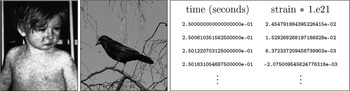
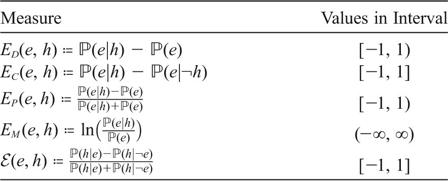
An objection to my point would be to claim that data are as epistemically accessible as the evidence 〈e _⋅〉. Figure 1 shows examples of sets of data that correspond to our examples 〈h _⋅〉 and 〈e _⋅〉. In this case, 〈d _⋅〉 does not denote a human-made proposition, it denotes the set of data itself that is relevant for scientific reasoning; $d_{\cdot }\in A$ denotes its representations in the probability space. Confronted with the complexity of the data—millions of perceptible pixels, thousands of numbers—there is no meaningful way in interpreting ℙ(d _⋅) with 〈d _⋅〉 being the actual set of data. How surprising is it to get exactly this picture of a raven or this series of numbers? That is why, in many realistic examples from science, evidence 〈e〉 in Bayesian frameworks, which make use of ℙ(e), cannot be observed data. Our brain is not designed to specifically focus on raw data, but in science we often do so. The inference from data to evidence is a crucial epistemic step in contexts of scientific explanations. The measures of explanatory power that Schupbach refers to (see table 1) take as explananda evidence and neglect the inference from data to evidence.

Figure 1.

Examples of data. (Sources: Wikimedia, http://pixabay.com, http://losc.ligo.org.)

Table 1.

Candidate Measures of Explanatory Power

Measure	Values in Interval
ED(e, h) ≔ ℙ(e|h) − ℙ(e)	[−1, 1)
EC(e, h) ≔ ℙ(e|h) − ℙ(e|¬h)	[−1, 1]
$E_P\left(e,h\right)≔\frac{\mathbb{P}\left(e|h\right)-\mathbb{P}\left(e\right)}{\mathbb{P}\left(e|h\right)+\mathbb{P}\left(e\right)}$	[−1, 1)
$E_M\left(e,h\right)≔\ln \left(\frac{\mathbb{P}\left(e|h\right)}{\mathbb{P}\left(e\right)}\right)$	(−∞, ∞)
$ℰ\left(e,h\right)≔\frac{\mathbb{P}\left(h|e\right)-\mathbb{P}\left(h|\neg e\right)}{\mathbb{P}\left(h|e\right)+\mathbb{P}\left(h|\neg e\right)}$	[−1, 1]

Note. Measures as listed by Schupbach (Reference Schupbach2011). We refer to his text for further historical references regarding these measures.

The representations of data 〈d _⋅〉 in figure 1 are to a certain degree still approximations. Digital images are restricted by their size in pixels, the data may more accurately be represented by a video, and so on. However, these approximations describe 〈d _⋅〉 much better than just identifying it with the propositional evidence 〈e _⋅〉.

Example 〈d_c〉 is of particular interest to us. In cases 〈d_a〉 and 〈d_b〉 the inferences from data to evidence can be explained by common sensitive-cognitive abilities and proper background knowledge about the discussed phenomena. These abilities cannot be described easily and raise scientific questions by themselves, but we can agree on their being natural capabilities of human beings and therefore reasonably addressed by $\mathbb{P}\left(e_{\cdot }|d_{\cdot }\right)$, which gives the degree to which the evidence can be inferred from the given set of data.

This description does not apply to 〈d_c〉. Here, the inference from data to evidence is based on an algorithm to detect the patterns that we can infer from Einstein’s theory of general relativity and our knowledge about cosmic bodies. Also relevant to the inference are controlling mechanisms to delete known disturbing influences from the data. The physicists present their results with quantifications of the degree of statistical certainty, which is common in experimental discoveries.Footnote ⁴ Expression ℰ(e_c, h_c) gives the explanatory power excluding this statistical uncertainty for the inference from 〈d_c〉 to 〈e_c〉. Probability $\mathbb{P}\left(e_c|d_c\right)$ is the degree to which 〈e_c〉 can be inferred from 〈d_c〉, and this probability is completely different from some degree of surprise that 〈e_c〉 occurs.

In many related discussions the difference between the evidence 〈e〉 and the set of data 〈d〉 is neglected. A common understanding seems to be that this inference can be neglected as a minor influence to scientific and everyday reasoning that becomes an insignificant victim in the process of approximation. Example 〈⋅_c〉 is associated with a history of false inferences from data to evidence,Footnote ⁵ or to say it more accurately: it is a history of overestimating the degree to which the evidence is given by the observed data or overestimating the degree to which 〈h_c〉 is true if some evidence is given. We elaborate on this history in section 6.

In Schupbach (Reference Schupbach2011) participants to an experiment have to provide personal degrees of belief after investigating a series of 10 balls that are drawn from an urn A and not from urn B. From both urns, they know the composition of black and white balls, and they are asked to decide from which urn the balls were drawn. An outcome of the draw is the finite information fully described by, for example, 〈e_s〉 bwwbwbbbbw. Here, $〈e_s〉=〈d_s〉$; in this example there is no difference between the evidence and the data, and no inference from data to evidence is necessary (or it is trivial). I take this choice of an example as an indication for the common negligence of the inference from data to evidence. Overall, this example is a very artificial simplification of actual scientific or everyday examples to which a measure of explanatory power should be applicable to.

3. Measures of Explanatory Power

Schupbach and Sprenger (Reference Schupbach and Sprenger2011) discuss measures of explanatory power. These measures provide a quantification (e.g., a value in the interval [−1,1]) of explanatory power that a hypothesis has over some evidence. Formally,

$E_{\mathbb{P}}\left(e,h\right):A^2\times P\to ℝ,$

with $P$ being the set of all probability measures over the measurable space (Ω, $A$). They provide a Bayesian account to answer questions like ‘how strongly does a measles infection explain a red rash?’. The measures explicate explanatory power in contexts of everyday and of scientific reasoning. Measures of explanatory power are already available in the literature, but Schupbach and Sprenger argue in favor of a new version, which they denote with “ℰ(e, h).” I use their result as a recently discussed example to further describe problems and suggest an adaptation that incorporates the distinction between evidence and data. A historical overview of some measures is given in table 1.

Schupbach and Sprenger claim that “our grasp on the notion of explanation is at least sufficiently strong to ground a precise formal analysis of explanatory power, even if it is not strong enough to determine a general account of the nature of explanation” (Reference Schupbach and Sprenger2011, 107). Their technique to define the measure ℰ(e, h) for a proposition e and a hypothesis h is to introduce a list of reasonable constraints that ℰ has to fulfill. These constraints express criteria of normalization and symmetry, as well as a proper interpretation of independencies between the relevant propositions.

To infer or explicate the different measures of explanatory power, the authors make use of several conditionalized and unconditionalized assignments of probabilities. They assign probabilities to the explanandum ℙ(e), to the explanandum constrained on the explanans $\mathbb{P}\left(e|h\right)$ and its negation $\mathbb{P}\left(e|\neg h\right)$, and to the explanans constrained on the explanandum $\mathbb{P}\left(h|e\right)$ and its negation $\mathbb{P}\left(h|\neg e\right)$. We have to consider these assignments, when we introduce d to the measure.

This new versionFootnote ⁶

${\widehat{ℰ}}_{\mathbb{P}}\left(d,e,h\right):A^3\times P\to ℝ$

aims to explicate the explanatory power of a hypothesis over some set of observed data, which, in many cases, cannot be interpreted as a special form of evidence. From a formal perspective, the cornerstone of $\widehat{ℰ}$ is to somehow incorporate the inference from data to evidence (e.g., by reference to $\mathbb{P}\left(e|d\right)$ and $\mathbb{P}\left(\neg e|d\right)$).

4. Explanatory Power and Data: Separating Data from Evidence

How can we adapt ℰ to measure the explanatory power that a hypothesis has over a set of observed data, instead of some propositional evidence? The intention for the adaptation is that we want to explain what we actually observe (or at least what we recorded from the observation) and provide a justified explication of this trivalent measure $\widehat{ℰ}\left(d,e,h\right)$.

The probabilistic expressions $\mathbb{P}\left(h|e\right)$ and $\mathbb{P}\left(h|\neg e\right)$ are the parameters of ℰ(e, h). Our approach for $\widehat{ℰ}$ is to adapt these building blocks for the measure of explanatory power over observed data accordingly. The first step is to adapt $\mathbb{P}\left(h|e\right)$ by formalizing the preformal intuition

to replace

from ℰ. The notation “ℙ(⋅[⋅]⋅)” is more or less arbitrary and is chosen to express the described intentions by syntactically replacing the conditionalization “|” with a conditionalization “[e]” in which we are implicitly restricted to a propositional evidence 〈e〉 at the inference from 〈d〉 to 〈h〉. The term “ℙ(⋅[⋅]⋅)” is only a notation and, as will become clearer below, I do not intend to extend the standard probability calculus in any way.

The evidence still plays an important role for $\widehat{ℰ}$. We aim to measure the explanatory power for a set of observed data via some evidence. In science, as well as in everyday explanations, data are always interpreted somehow; we have to know what we look for in the data. In many realistic scientific examples, the evidence (e.g., patterns from gravitational waves) for which we look in the data (e.g., time series from LIGO measurement) is already well described before the data are gathered. This may even be seen as a indicator of good scientific method. Furthermore, if we imagine a case of Popperian falsification (see sec. 7.3), evidence may also be chosen with a particularly negative relevance to the hypothesis in question. Evidence can, roughly speaking, be explicated in the language of hypothesis confirmation or falsification, whereas data cannot (at least not in a direct way); our cases 〈h _⋅〉, 〈e _⋅〉, and 〈d _⋅〉 provide examples for this. A set of data cannot be the explanandum of an explanation without the stipulation of some propositional evidence that should be revealed in the data by some pattern.

My technique to explicate ℙ(h[e]d) is to, first, list constraints that are necessary to really express the intention as preformally described above. We establish the following constraints for

$\mathbb{P}\left(h\left[e\right]d\right):A\times A\times A\to [0,1]$

and all h, h ₁, h ₂, e, d, d ₁, $d_2\in A$ and $D,\mathscr{H}\subset A$:

(i)	Informativeness:	ℙ(h), ℙ(e), $\mathbb{P}\left(d\right)\in \left(0,1\right)$, that is, open intervals
(ii)	Evidential Data:	If $e=d$, then $\mathbb{P}\left(h\left[e\right]d\right)=\mathbb{P}\left(h|e\right)$
(iii)	Weak Data:	$\mathbb{P}\left(h\left[e\right]d\right)\le \mathbb{P}\left(h|e\right)$
(iv)	Independence:	If $\mathbb{P}\left(e|\overline{d}\right)$ is constant for all $\overline{d}\in D$, then $\mathbb{P}\left(h\left[e\right]{\overline{d}}_1\right)=\mathbb{P}\left(h\left[e\right]{\overline{d}}_2\right)$ for all ${\overline{d}}_1,{\overline{d}}_2\in D$, and if $\mathbb{P}\left(\overline{h}|e\right)$ is constant for all $\overline{h}\in \mathscr{H}$, then $\mathbb{P}\left({\overline{h}}_1\left[e\right]d\right)=\mathbb{P}\left({\overline{h}}_2\left[e\right]d\right)$ for all ${\overline{h}}_1,{\overline{h}}_2\in \mathscr{H}$
(v)	Monotonicity:	If $\mathbb{P}\left(e|d_1\right)\le \mathbb{P}\left(e|d_2\right)$, then $\mathbb{P}\left(h\left[e\right]d_1\right)\le \mathbb{P}\left(h\left[e\right]d_2\right)$, and if $\mathbb{P}\left(h_1|e\right)\le \mathbb{P}\left(h_2|e\right)$, then $\mathbb{P}\left(h_1\left[e\right]d\right)\le \mathbb{P}\left(h_2\left[e\right]d\right)$

The intentions concerning the constraints are mostly self-explanatory. We introduce i to exclude tautologies and contradictions and to avoid division-by-zero problems. Constraint ii aims to cover the—often very artificial—examples in which the data are already designed to be evidence. Constraint iii expresses that the assumption of 〈e〉 (or $〈e〉=〈d〉$) always nondecreases the ℙ(h[e]d), since the inference from 〈d〉 to 〈h〉 is restricted to only infer 〈e〉 (and no other possibly evidence) from 〈d〉. Constraint iv states that the two steps, inference from data to evidence and inference from evidence to hypothesis, are statistically independent. Constraint v expresses that ℙ(h[e]d) increases, if one of the two relevant degrees of inference increase with the other one being constant.

Remark A solution consistent with constraints ii–v for all probability spaces (Ω, $A$, ℙ) and all h, e, $d\in A$ for which i holds is

$\mathbb{P}\left(h\left[e\right]d\right)≔\mathbb{P}\left(h|e\right)\cdot \mathbb{P}\left(e|d\right).$

This solution for ℙ(h[e]d) is the one we use in the following course of this article. Note that this remark does not imply uniqueness of the solution. I intentionally introduced the intuitive notation ℙ(h[e]d) despite the simple alternative given by this definition. However, when it comes to estimating ℙ(h[e]d) in empirical contexts (i.e., degrees of belief or truth or appropriateness), cases may occur in which we estimate ℙ(h[e]d) directly without a further analysis of its mathematical structure.

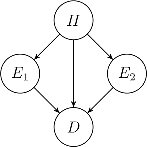
The probabilistic models for ℰ and $\widehat{ℰ}$ imply specific probabilistic dependencies between the set of observed data, the evidence, and the hypothesis. The Bayesian networks shown by figure 2 provide an accessible approach to express these dependencies.Footnote ⁷ The notation with capitalized letters is common in the literature on Bayesian networks.Footnote ⁸

Figure 2.

Bayesian networks that describe the underlying dependencies. Left, Schupbach and Sprenger’s binary relation between hypothesis and evidence, as implied by ℰ. Right, my trivalent approach with data, as regarded by $\widehat{ℰ}$.

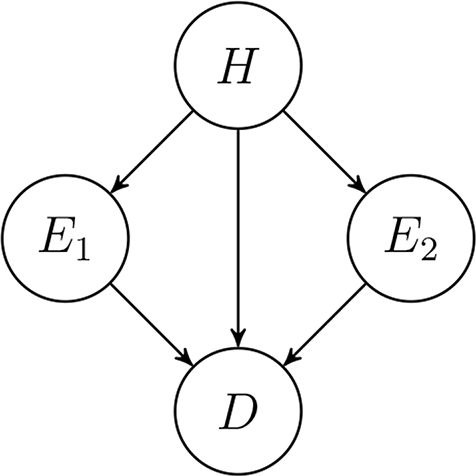
Figure 2, right side, indicates how the inference from hypothesis to data depends on a specific evidence. Note that for $\widehat{ℰ}\left(d,e,h\right)$ the inference from 〈d〉 to 〈h〉 (which is represented by the arrow from H to D) is irrelevant. This evidence in many cases in science is described before the observation or gathering of the data. Figure 3 shows a simple example to highlight these aspects and how our invention $\widehat{ℰ}$ can capture it properly, whereas ℰ cannot. In this example, if we measure very precisely, $\widehat{ℰ}\left(d,e_2,h\right)$ is high, but $\widehat{ℰ}\left(d,e_1,h\right)$ is not, and the reason is, of course, the different appropriateness of the choice of the evidence. Note that the amount of alternative evidence is high or even infinite.

Figure 3.

Bayesian network for 〈h〉, the earth rotates around the sun; 〈e ₁〉, pattern of a round orbit; 〈e ₂〉, pattern of a nonround elliptic orbit; and 〈d〉, records of the sun’s position. The actual orbit is nonround elliptic.

5. Explanatory Power and Data: Constructing the Adapted Measure

To replace the expressions $\mathbb{P}\left(h|e\right)$ and $\mathbb{P}\left(h|\neg e\right)$ from ℰ to a three-placed probabilistic expression over d, (¬)e, and h and to express the measure of explanatory power for a set of data, we need to answer the following question. How do we translate the conditional probability $\mathbb{P}\left(h|\neg e\right)$ from ℰ into our trivalent version, if $\mathbb{P}\left(h|e\right)$ translates to the ℙ(h[e]d) as discussed above?

By constraints iv and v, ℙ(h[e]d) can only be a high value if $\mathbb{P}\left(h|e\right)$ and $\mathbb{P}\left(e|d\right)$ are high values. In contrast, the trivalent adaptation of $\mathbb{P}\left(h|\neg e\right)$ should be high, if either $\mathbb{P}\left(h|\neg e\right)$ or $\mathbb{P}\left(\neg e|d\right)$ is high. The reason for this is that to achieve high explanatory power the negated evidence should neither lead to a high support of the hypothesis nor be strongly supported by the data. A simple solution to formalize this intuition is to translate $\mathbb{P}\left(h|\neg e\right)$ for the trivalent adaptation into $\max \left(\mathbb{P}\left(h|\neg e\right),\mathbb{P}\left(\neg e|d\right)\right)$. Note that the calculations made in the case study about gravitational waves in section 6 further illuminate these intuitions and formalization.

Note that 〈¬d〉 expresses, strictly speaking, every possible outcome of the measurement except the very specific set of data 〈d〉. Since 〈d〉 includes one specific realization of noise and ℙ(d) is a very low value, 〈¬d〉 does not have any useful meaning for our approach. In an empirical setup of explanatory power, 〈d〉 solely plays the role to confirm or disconfirm some specified evidence 〈e〉 to a certain degree (i.e., $\mathbb{P}\left(e|d\right)$ or $\mathbb{P}\left(\neg e|d\right)$).

We can now explicate the measure of explanatory power of a hypothesis 〈h〉 over a set of observed data 〈d〉 via some evidence 〈e〉:

$\widehat{ℰ}\left(d,e,h\right)=\frac{\mathbb{P}\left(h\left[e\right]d\right)-\max \left(\mathbb{P}\left(h|\neg e\right),\mathbb{P}\left(\neg e|d\right)\right)}{\mathbb{P}\left(h\left[e\right]d\right)+\max \left(\mathbb{P}\left(h|\neg e\right),\mathbb{P}(\neg e|d)\right)}.$

This adaptation makes use of the advantages of ℰ over the alternative measures of explanatory power (see table 1) by the adaptation of its basic structure. However, from a semantic perspective and concerning the derivation of the measure analogous to Schupbach and Sprenger’s, we do something substantially different: the explanandum does not need to be some proposition 〈e〉. In our account the explanandum can also be a set of observed data 〈d〉.

The occurrence of the maximum operator at $\widehat{ℰ}$ may seem unpleasant from an analytical mathematical perspective, since it makes $\widehat{ℰ}$ nondifferentiable. The intuition behind it is that, again, first, ℰ gets significantly negative or close to zero, if $\mathbb{P}\left(h|\neg e\right)$ is high. Second, at $\widehat{ℰ}$ this can occur in two different ways, which are a high value for $\mathbb{P}\left(h|\neg e\right)$ or a high value for $\mathbb{P}\left(\neg e|d\right)$. This aims to ensure that $\widehat{ℰ}$ cannot be high, if one of these two scenarios occurs. Note that one of these two values being high should lead to a significantly low explanatory power—the examples “weak evidence in strong data” and “strong evidence in weak data” in section 6 exemplify this point. And this desired feature is exactly what the maximum operator expresses, whereas there is no philosophical need for $\widehat{ℰ}$ to be differentiable.

Schupbach and Sprenger’s ℰ is taken as a template for my adaptation because of the normative arguments they give in addition to Schupbach’s (Reference Schupbach2011) empirical arguments. These are that ℰ performs best among the candidate measures according to an empirical investigation of decisions from 26 participants. However, if you take a more critical perspective on ℰ, my preformal discussion and some aspects of the formalization of $\widehat{ℰ}$ may also be picked up to define adaptations of the other measures that are listed in table 1 to incorporate the distinction between evidence and data. However, the notation “$\widehat{ℰ}$” is justified by the fact that for $e=d$ we have $\widehat{ℰ}{|}_{e=d}\left(d,e,h\right)\equiv ℰ\left(e,h\right)$.

6. A Comparison of ℰ and $\widehat{ℰ}$: The Example of Gravitational Waves

We briefly discuss the historical example of the detection of gravitational waves (GW) to show how our approach for $\widehat{ℰ}$ is applicable and very appropriate for explicating explanatory power. GW are a theoretical result from general relativity that also allows for the possibility of detection by various ways. I mention several observations or measurements to detect GW and how the explanatory power of the theory of general relativity over the measurement results is reflected by $\widehat{ℰ}$.Footnote ⁹

I suggest some very rough probability assignments for the application of ℰ and $\widehat{ℰ}$. These assignments aim to highlight the implications of $\widehat{ℰ}$ rather than being perfectly accurate under all possible considerations, which demands a more lengthy discussion. Furthermore, the probability assignments are very conservative in the sense that, for instance, “very strong” translates to 0.95 to make the calculations more accessible, whereas in actual experimental physics “very strong” would rather translate to $0.99\overline{9}$. In what follows, 〈h〉 denotes the hypothesis that GW exist, and ℙ are the degrees of belief of the mainstream gravitational physicists community.

6.1. Weak Evidence in Strong Data: Rotating Cylinders

The physicist Joseph Weber detected expansions and contractions of a heavy solid cylinder when another heavy solid cylinder rotated in an orthogonal position to it (〈e_W〉). He first conducted experiments of this kind in the late 1960s, and other physicists repeated modernized versions of the experiment until the year 2000. The data showed clear effects, and Weber claimed that this evidence confirms GW. His critics claim that this effect can be explained by gravitation alone without the assumption of GW. They claim that the detected effect is similar to tides on earth that are caused by the moon’s gravitation. The majority of physicists who work on GW criticize Weber’s conclusion. Let 〈d_W〉 denote his measurement results:

$\mathbb{P}\left(h|e_W\right)=P\left(h|\neg e_W\right)=\mathbb{P}\left(h\right)=.5,\mathbb{P}\left(e_W|d_W\right)=.95,\mathbb{P}\left(\neg e_W|d_W\right)=\mathrm{.05.}$

The value for ℙ(h) depends a lot on the point in time (e.g., before or after certain other discoveries), and .5 is more or less arbitrarily chosen, not close to 0 or 1. This gives

$\widehat{ℰ}\left(d_W,e_W,h\right)=\frac{.5\cdot .95-\max \left(.5,.05\right)}{.5\cdot .95+\max \left(.5,.05\right)}\approx \mathrm{-.026}\approx 0.$

It gives $ℰ\left(e_W,h\right)=0$, as well, but our approach makes clear that this low explanatory power is due to the interpretation of the experimental results and not due to unsatisfying measurement results.

6.2. Medium-Strong Evidence in Strong Data: Orbit Degradations

Hulse and Taylor (Reference Hulse and Taylor1975) measured orbits of a binary star system and detected degradations, which are consistent with the energy loss explained by GW. This evidence is considered strongly confirmed by the data but not very reliable because of strong additional background assumptions for the interpretation of the measurements.Footnote ¹⁰ Their set of data is 〈d _HT〉, and their evidence is 〈e _HT〉.

$\begin{array}{c}\mathbb{P}\left(h|e_{\mathrm{HT}}\right)=.8,P\left(h|\neg e_{\mathrm{HT}}\right)=.4,\mathbb{P}\left(e_{\mathrm{HT}}|d_{\mathrm{HT}}\right)=.95,\mathbb{P}\left(\neg e_{\mathrm{HT}}|d_{\mathrm{HT}}\right)=.05\\ \widehat{ℰ}\left(d_{\mathrm{HT}},e_{\mathrm{HT}},h\right)=\frac{.8\cdot .95-\max \left(.4,.05\right)}{.8\cdot .95+\max \left(.4,.05\right)}\approx .31\end{array}$

is, again, close to $ℰ\left(e_{\mathrm{HT}},h\right)=1/3$. This is always the case for the strong data examples but not for weak data.

6.3. Strong Evidence in Weak Data: Early Interferometers

The two LIGO interferometers are active in the search for GW since 2002. Interferometers provide measurement data for the detection of GW and are widely accepted as actually doing so in the physicists mainstream community. After finding that the data (〈d _L02〉) are too noisy to detect possible signs of GW (〈e _L〉), the more sensitive Advanced LIGO was put into operation in 2015. For the early LIGO, we have

$\begin{array}{c}\mathbb{P}\left(h|e_L\right)=.99,P\left(h|\neg e_L\right)=.02,\mathbb{P}\left(e_L|d_{L02}\right)=.5,\mathbb{P}\left(\neg e_L|d_{L02}\right)=.5\text{, and}\\ \widehat{ℰ}\left(d_{L02},e_L,h\right)=\frac{.99\cdot .5-\max \left(.02,.5\right)}{.99\cdot .5+\max \left(.02,.5\right)}\approx .005\approx 0\text{, but}\end{array}$

$ℰ\left(e_L,h\right)\approx .96$, and ℰ(d _L02, h) is not determinable by the problems of interpreting $\mathbb{P}\left(h|d\right)$, which we discussed in section 2.2.

6.4. Strong Evidence in Strong Data: LIGO 2015 Interferometers

Recently, with a stated degree of $\mathbb{P}\left(e_L\right|d_{L15})\in (0.99,1)$, reliable confirmation of GW was published by Abbott et al. (Reference Abbott2016). With the assignments that we know from the case before this one, we get

$\widehat{ℰ}\left(d_{L15},e_L,h\right)=\frac{.99\cdot .995-\max \left(.02,.005\right)}{.99\cdot .995+\max \left(.02,.005\right)}\approx \mathrm{.96.}$

Without the separation of evidence and data, we are not able to distinguish between some profoundly different scenarios. Strongly explained evidence may be given only weakly in data, and weakly explained evidence may strongly be inferred from the data. For ℰ these different effects have to be semantically incorporated into the evidence 〈e〉, which leads to unreasonable and indeterminable probability assignments.

7. Further Comments on History and Applicability

In the introduction and other parts of the article, I make several remarks about the history of the distinction between data and evidence. In this section, I offer a more thorough discussion on this matter and on the actual applicability of constraint v.

7.3. Popperian Falsification and $\widehat{ℰ}$

A further strength of my suggested measure of explanatory power $\widehat{ℰ}\left(d,e,h\right)\in \left[\mathrm{-1},1\right]$ is the result that it provides for cases of falsification, as discussed by Popper (Reference Popper1935). If a set of data provides strong support for falsifying evidence, then the explanatory power of the falsified hypothesis should be close to −1.

This is a classical example:

〈h〉 Light propagates linearly through space without being influenced by gravitation.

〈e〉 Stars at daytime with an eclipsed sun appear in the same arrangement as in earth’s night sky.

After waiting for a proper sun eclipse to gain the desired image 〈d〉, 〈h〉 was considered to be falsified because of strong support for 〈¬e〉 by 〈d〉. In Bayesian terms, this leads to something very roughly like

$\mathbb{P}\left(e|d\right)=.01,\mathbb{P}\left(\neg e|d\right)=.99,\mathbb{P}\left(h|\neg e\right)=.01,\mathbb{P}\left(h|e\right)=.9,$

and

$\widehat{ℰ}\left(d,e,h\right)=\frac{.01\cdot .9-\max \left(.01,.99\right)}{.01\cdot .9+\max \left(.01,.99\right)}=\frac{.009-.99}{.009+.99}=\frac{\mathrm{-.981}}{.999}\approx \mathrm{-.98.}$

This result corresponds perfectly with a possible notion of a degree of falsification (modulo a change of sign).

8. Implications for Measures of Confirmation

Expression “ℙ(h[e]d)” denotes the intuition that any positive inference from data to a hypothesis is only possible by the stipulation of some evidence. This fact influences not only the discussion about measures of explanatory power but also the discussion about measures of confirmation of a hypothesis by some scientific observational result. As opposed to the measures of explanatory power that are listed in table 1, measures of confirmation from the recent literature often take into account that confirmation could be a three-placed relation between evidence 〈e〉, hypothesis 〈h〉, and some auxiliary hypotheses and assumptions 〈k〉.Footnote ¹³

In Crupi’s (Reference Crupi and Zalta2015) notation with variable names as given above, a degree of confirmation is

$C_{\mathbb{P}}\left(h,e|k\right):A^3\times P\to ℝ,$

with $P$ being the set of all probability measures over the measurable space (Ω, $A$). This notation also implies that 〈k〉 with $k\in A$ and $\mathbb{P}\in P$ are assumed to be given when the degree of confirmation is measured.

How would a ${\hat{C}}_{\mathbb{P}}\left(h,e,d|k\right)$ that makes use of the idea ℙ(h[e]d) look? A full answer to this question is part of this article and demands an elaborated discussion of its own. But at this point we can speculate how relevant our discussion for $\widehat{ℰ}$ is for ${\hat{C}}_{\mathbb{P}}\left(h,e,d|k\right)$. The original intentions for the introduction of the auxiliaries 〈k〉 include the problem that what is often referred to as “evidence” is hardly logically formulated or expressible and fits more the notion of data as introduced in this article. However, the issue that one set of data can confirm a hypothesis to different degrees depending on the choice of the evidence is still not addressed with the introduction of auxiliaries at $C_{\mathbb{P}}\left(h,e|k\right)$. The Bayesian network from figure 3 exemplifies this point for confirmation, too. That is why ${\hat{C}}_{\mathbb{P}}$ has to deviate from C _ℙ by philosophical intentions similar to those underpinning how $\widehat{ℰ}$ deviates from ℰ.

9. Conclusion

Approaches to model explanatory power stipulate propositional evidence as explananda. I claim that—in opposition to the vast majority of the tradition of this discussion—observed data are the more adequate explanandum for many scientific applications.

We inferred that for a measure of explanatory power a distinction between evidence and data must be represented in a mathematical explication, which is $\widehat{ℰ}$. Measure $\widehat{ℰ}$ is a relatively simple adaptation of Schupbach and Sprenger’s suggested measure ℰ. The adaptation $\widehat{ℰ}$ solves the problem of the separation of evidence from data.

The construction of $\widehat{ℰ}$ is based on a list of constraints. These constraints include, first, that, even if we are interested in the explanatory power of a hypothesis for a set of observed data, it can—by epistemic reasons—only be inferred with the stipulation of some specified evidence in it. Second, we refer to $\mathbb{P}\left(e|d\right)$ in $\widehat{ℰ}$ to explicate how strongly evidence can be inferred from the set of data under investigation.

We discussed the example of gravitational waves to highlight the importance of the separation of evidence and data for the application of measures of explanatory power. The argument applies to everyday examples, too. The arguments that were raised in favor of a distinction between evidence and data for the explication of explanatory power similarly apply to explications of measures of confirmation.