LITERATURE REVIEW

The debate on the causes of the North-South gap, the so-called “questione meridionale,” is almost as old as Italy as a unified state (Felice Reference Esposto2007).Footnote ¹ The debate has, surely, been rich in ideas and conjectures, as testified, for example, by the opposed views proposed by Luciano Cafagna (Reference Cafagna and Cafagna1962, Reference Cafagna1971) and Edmondo Capecelatro and Antonio Carlo (Reference Capecelatro and Carlo1972). The former argued that the Northwest industrialized because it had much greater development potential than any other region, with minimal economic interactions with the South; while the latter denied the existence of a North-South gap at the time of the Unification. The Cafagna interpretation implies that the gap was already large and possibly centuries old, while for Capecelatro and Carlo (Reference Capecelatro and Carlo1972) it was created by the policies of the newly unified Italy. However, until recently, the debate remained unsettled for lack of data. Early estimates of regional GDP (Eckhaus Reference Daniele and Malanima1961; Zamagni 1978; Esposto Reference Esposto1997) were very tentative and were mostly ignored by the literature, which relied almost exclusively on anecdotal evidence.

The debate on the causes of the gap has been reinvestigated in recent years. Brian A’Hearn and Anthony Venables (Reference A’Hearn, Venables and Toniolo2013), in a broad new economic geography framework, have suggested that the North was richer than other regions at the time of the Unification thanks to its geographical advantages. It had more water, it was more suited for the production of silk, Italy’s main staple product, and after 1890, it benefitted from protectionist policies and increasing market access. In the same year, Emanuele Felice (Reference Federico2013) argued for a major role played by institutions along the lines of the Daron Acemoglu and James Robinson (Reference Acemoglu and Robinson2012) dichotomy of “inclusive” versus “extractive” institutions. The Southern élites resisted any change that could jeopardize their political power—most notably investment in education and health (Felice and Vasta Reference Federico2015). In contrast, Carlo Ciccarelli and Stefano Fenoaltea (Reference Ciccarelli and Fenoaltea2013) tentatively suggested that market-integrating policies, abolishing of borders and railway construction, could explain industrial growth at least in some provinces of the South after the Unification.

These conjectures have been subject to econometric testing using three different measures of performance: GDP per capita by region (Brunetti, Felice and Vecchi Reference Brunetti, Felice, Vecchi and Vecchi2011), the share of industrial occupation from population censuses (Ciccarelli and Missiaia Reference Cha2013), and labor productivity in manufacturing by province (Ciccarelli and Fenoaltea Reference Cappelli2013). Felice (Reference Felice2012) uses the first (GDP per capita) to argue that the growing North-South divergence before WWI depended on differences in endowment of human capital. This hypothesis is also supported by the results presented by Gabriele Cappelli (Reference Bolt and van Zanden2016) and Cappelli and Michelangelo Vasta (Reference Cappelli and Vasta2017) on the positive effect on school enrollment in the South with the Daneo-Credaro Law (1911) that shifted the organization and the funding of primary school from local authorities, often very poor, to the state. Other works have stressed the role of geographical factors and especially of market potential. Anna Missiaia (Reference Missiaia2016) finds some evidence for a positive role of domestic market access for the development of the North that were, however, compensated by better access to the world market for the South. Vittorio Daniele, Paolo Malanima, and Nicola Ostuni (Reference Daniele, Paolo and Ostuni2018) confirm the positive effect of market access on the share of industrial occupation by province for benchmark years from 1911 to present, but in their estimates the North had greater domestic and foreign market potential than the South. Roberto Basile and Ciccarelli (Reference Basile and Carlo2018) also find a positive effect of market potential and literacy on the industrial provincial location of different sectors.

All studies on the causes of productivity growth in manufacturing single out human capital as a key driver, but they disagree on the role of other determinants. Cappelli (Reference Cappelli2017) and Alessandro Nuvolari and Vasta (2017) find evidence of a positive role of innovative activity, measured by patent data, while Ciccarelli and Stefano Fachin (Reference Ciccarelli and Fachin2017) identify social capital as a major cause. However, this latter result is not confirmed by Cappelli (Reference Cappelli2017) using different measures of social capital. In all these contributions, other variables, such as infrastructures, water resources, and market access, tend not to be significant.

These quantitative articles have undoubtedly increased our understanding of the origins and causes of the Italian regional divide, but, unfortunately, all these contributions are still based on somewhat fragile data. The regional GDP data refer only to benchmark years and, more importantly, they do not cover the key period after Unification; moreover, they are quite controversial as shown by the recent debate between Felice (Reference Giovanni and Rey2014) and Daniele and Malanima (Reference Daniele and Malanima2014a, Reference Daniele and Malanima2014b). The estimates of labor productivity not only rely on some specific assumptions, but also industry accounted only for one-fifth of Italian GDP in 1891 and 1911 (Rey 2002, Tabs. 2 and 3).

When data on economic performance are missing or dubious, proxies have been used. Looking at the results of recent works, we find the North well ahead of the South on social indicators such as heights (A’Hearn and Vecchi 2017), life expectancy, and Human Development Index (HDI) (Felice and Vasta Reference Federico2015) and also social capital (Felice Reference Felice2012; Cappelli Reference Brunetti, Felice, Vecchi and Vecchi2017).Footnote ² Moreover, the strikingly large and persistent differences in literacy rates are particularly relevant given the key role of human capital for economic growth. All these data would support the traditional thesis about the causes of the North-South divide, but they are surely not conclusive evidence, as the correlation between economic performance indicators and social indicators is far from perfect (van Zanden et al. Reference van Zanden, Baten and Mira d’Ercole2014).

In this context of weak data, to provide insights on the origins of the North-South, one can follow the stream of international literature that has used real wages as proxy of economic performance. Until now, there were no series of real wages by regions for the period from Unification to WWI. There were several national series, from the pioneering work by Alberto Geisser and Effren Magrini (Reference Geisser and Effren1904), to the more recent works by Vera Zamagni (Reference Zamagni1984, Reference Zamagni and Scholliers1989) for industrial workers from 1890 to 1913, Giovanni Federico (Reference Federico1994, p. 574) for female silk reelers from 1861 to 1913, and Fenoaltea (Reference Fenoaltea1985, Reference Fenoaltea2002) for construction workers. There is one set of provincial wages, for construction workers, but it covers only the period 1862–1878 (Daniele and Malanima Reference Cvrcek2017).Footnote ³ Consistent with their overall view of the North-South divide, the authors find no evidence of a North-South gap immediately after the Unification. If anything, wages of construction workers were higher in the South (including islands) than in the North-Centre, although the difference was within the margin of error of the estimates. Daniele and Malanima find that wages in the North-Centre rose relative to Southern wages from the late 1860s.

Against this background, the present article is the first systematic attempt to deal with trends in provincial wages for the whole first phase of Italian industrialization from the Unification to WWI.

SOURCES AND METHODS

We estimate Italian provincial real wages according to the Allen (Reference Allen2001) original method. This implies calculating the annual income of a worker taking into account wages and working days and dividing it by a bare bones basket. Allen (Reference Allen2001) defines the WR as:

(1) $$WR = {{W \cdot N} \over {\sum\nolimits_{j = 1}^K {{P_j} \cdot {Q_j}} }} \cdot {1 \over D},$$

where W = daily wage for male worker, N the number of days worked, D is the number of members of the household in consumption units, P_j is the price of the j-th good, and Q_j the fixed quantity of the j-th good. If WR = 1 the male breadwinner wage is exactly sufficient to sustain the household.

Allen (Reference Allen2001) suggested using two sets of WRs, corresponding respectively to a mere subsistence (the “bare bones” basket) and to a slightly better standard of living (the “respectable” basket). The former is designed to give each consumption unit the minimum amount of food for work, at the lowest possible cost, plus the barest minimum for lodging, clothing, and fuel. Allen suggested a minimum of 1,940 calories and, lacking information, assumed 250 days of work (5 days for 50 weeks) and an average household of four members, the male breadwinner, his wife, and two children—for a total of three consumption units. He then added rent as a markup of 5 percent to the cost of the basket, yielding a total of 3.15 baskets per household. This has become an international standard.Footnote ⁴

We estimate separate series for 69 provinces (for a detailed list, see Table A1 in Online Appendix A), which we aggregate by region and macro-area (Northwest, Northeast, Centre, South, Islands) as:

(2) $$WR = \sum\nolimits_{i = 1}^M {{s^i}} {{{W^i} \cdot {N^i}} \over {\sum\nolimits_{j = 1}^K {{P_j} \cdot {Q_j}} }} \cdot {1 \over D},$$

where sⁱ is the share of the i-th province on the total population of the relevant area (region or macro-area) according to population censuses (MAIC 1864–1865, 1874–1876, 1885, 1901–1904, 1914–1916) linearly interpolated. All our parameters, except the number of members of households (D), are, in principle, province specific.Footnote ⁵ In particular, we use the information of the number of days worked in each province as reported in an official enquiry of the early 1870s (MAIC-DGA 1876–1879).Footnote ⁶ The provincial data range from a minimum of 192 working days (Cagliari) to more than 300 in few provinces. The national average, simple (251.3) and weighted by population (253.3), is actually very close to Allen’s standard of 250 days of work per year, which we use for the international comparisons.Footnote ⁷ However, these differences would not matter substantially for the annual income, since the correlation between the two versions of annual income (with Allen standard and with province specific data of working days) is 0.925.

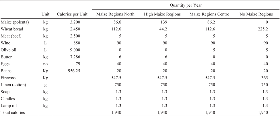
Our bare bones baskets differ across provinces in order to take into account traditional differences in dietary habits (Betri Reference Betri, Capatti, De Bernardi and Varni1998; Teti Reference Teti, Capatti, De Bernardi and Varni1998).Footnote ⁸ Northerners used butter rather than oil and ate much more polenta (a kind of maize gruel) than Southerners, as shown by the composition of gross output of cereals (Federico 1992, Reference Federico and Rey2000). Therefore, we use different bare bones baskets for: (i) Northern regions that were “regular” consumers of maize; (ii) Northern regions that were “intensive” consumers of maize; (iii) Central regions whose diet comprised of some maize; and (iv) Southern and Central regions where maize was not part of the diet (Table 1). Furthermore, we take into account differences in climate across regions assigning larger quantity of firewood to the cooler areas in the North. For international comparisons only, we have constructed a simplified bare bones basket as in Allen et al. (Reference Allen, Bassino and Ma2011), which assumes that the calories come mainly from the cheapest cereal, with the minimum amount of other food items to provide the physiological requirements of fats and proteins for survival. Thus, in this particular exercise, we substitute all calories from wine, eggs, and half of those from butter and oil olive with the cheapest cereal available in different macro-areas, maintaining the total amount of 1,940 calories.

Table 1

REGIONAL BARE BONES BASKETS FOR ITALY

Notes: Calories per unit are based on Malanima (Reference Humphries and Weisdorf2015). High maize regions: Lombardy and Venetia; maize regions of the North: Piedmont and Emilia; maize regions of the Centre: Marches, Abruzzi, and Umbria; no maize regions: Liguria, Tuscany, Latium, Campania, Apulia, Basilicata, Calabria, Sardinia, and Sicily.

Source: Authors’ own elaborations.

We estimate daily wages (wⁱ) and prices ($P_j^i$) from a variety of (mostly official) sources with details reported in Online Appendix B. We use two main sources for nominal wages of unskilled workers—an enquiry on wages paid by state for public works (MAIC-DGS n.d.) and the monthly Bollettino dell’Ufficio del Lavoro (MAIC ad annum). From the former, we obtained yearly averages of daily wages for navvies (terraiolo) in all Italian provinces (except Parma) from 1862 to 1878. In contrast, we have had to estimate the yearly income of unskilled agricultural workers by using monthly wage data for a large number of specific agricultural tasks, from 1905 onwards, from the Bollettino dell’Ufficio del Lavoro, combining these data with information about the composition of agricultural gross output and the number of days worked for each product given the prevailing technology.Footnote ⁹ Although our series refer to two different sectors, we are confident that the market for unskilled workers was integrated enough for this exercise. Our estimates for the period 1879–1904 ought to be considered more tentative. We were able to find suitable wage data only for 27 provinces (5 in the Northwest, 2 in the Northeast, 1 in the Centre, 12 in the South, and 7 in the Islands). We test the size of the potential bias by computing a new wage series for 27 provinces in 1862–1878 and 1905–1913 and comparing it with our baseline series (with all 69 provinces). The series match in the South and Islands (coefficients of correlation 0.997 and 0.994, respectively), are very similar in the Northwest (0.988) and in the Northeast (0.966), and show a lower but still strong correlation in the Centre (0.893).

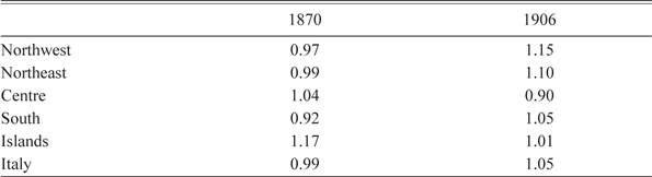
We perform two additional robustness checks on the level of wages, relying on two other official publications: the already quoted enquiry on agricultural wages in the early 1870s (MAIC-DGA 1876–1879) and an enquiry on wages of construction workers in 1906 (MAIC 1907).Footnote ¹⁰ We compute the ratios to our wages weighting the provincial data with the population (Table 2). Results are satisfactory: the nationwide gap is rather small and constant along time, and also the regional ratios do not differ much from 1, with the exceptions of the Islands in 1870 and of the Northwest in 1906. This suggests a fairly high degree of integration in the local labor markets.

Table 2

RATIO BETWEEN NOMINAL WAGES FROM DIFFERENT SOURCES FOR 1870 AND 1906

Sources: 1870 refers to the ratio between MAIC-DGS (nd) and MAIC-DGA (1876–1879); 1906 refers to the ratio between MAIC (ad annum) and MAIC (1907).

Our main sources for prices are for 1862–1873 MAIC-DGS (1886), for 1874–1896 the weekly Bollettino settimanale dei prezzi (MAIC-DGS ad annum), and for 1897–1913 MAIC (1914). MAIC-DGS (1886) reports wholesale prices for wheat, wine, olive oil, and corn and retail price of meat from 1862 to 1885 for a varying number of provinces—up to 23 for wheat.Footnote ¹¹ The Bollettino covers all provinces and reports retail prices of bread and meat and wholesale prices of wine, corn, olive oil, and firewood from 1880. MAIC (1914) reports the prices paid for bread, wine, olive oil, meat, butter, and eggs by the Convitti nazionali (boarding schools), which were probably somewhat lower than retail prices for ordinary consumers. When direct observations of bread prices are lacking, we convert wheat prices into bread prices by estimating a “bread equation” (Allen Reference Allen2001):

(3) $$Pbrea{d_i} = \alpha + \beta Pwhea{t_i} + \sum\limits_{i = 1}^K {{\gamma _i}provinc{e_i}} + {\sum\nolimits_{j = 1}^T {{\delta _j}year} _j},$$

where Pbread_i is the price of bread and Pwheat_i is the price of wheat in province i, and province_i and year_j are provincial and yearly dummies. We estimate the bread equation with data on bread and wheat prices for the period 1880–1896 (MAIC-DGS ad annum) with different specifications. Our preferred estimation yields a coefficient of β = 0.485 (Table B1 in Online Appendix B).

We estimate regional prices for fava beans by applying the difference in levels in the 1850s (Bandettini Reference Bandettini1957; Felloni Reference Felloni1957; Delogu Reference Delogu1959) to the nationwide series from ISTAT (1958). Unfortunately, we have not been able to find regional prices for lamp oil, candles, soap, and cotton cloth. We use the series from ISTAT (1958) for the first three items, while, for cotton cloths, we adjust the price of cotton yarn from Ernesto Cianci (Reference Capecelatro and Carlo1933) for 1870–1913 and then extrapolate the resulting series back to 1862 using the price of raw cotton in the United Kingdom from Brian Mitchell (Reference Linari1988). Calculating a single nationwide series for these items of the bare bones basket for all provinces might result in some spurious reduction of the variance of our price index. However, these goods accounted for a very small share of total expenditure and, thus, the distortion is likely to be very small. Finally, following Allen (Reference Allen2001), we add 5 percent to the cost of basket for rent.

Summing up, we have fairly detailed and reliable data on prices for the whole period, and, in particular, for the period 1874–1896. In contrast, the data on nominal wages are complete for the initial (1862–1878) and final (1905–1913) periods, but for the intervening period they are the result of the collation of somewhat heterogeneous sources, and, for this reason, as we have already noted, are more tentative. Furthermore, by construction, the Allen method rules out substitution among goods when relative prices change. Therefore, yearly series are bound to fluctuate widely when individual prices of major items in the basket are characterized by high volatility.

TRENDS IN REAL WAGES IN COMPARATIVE PERSPECTIVE

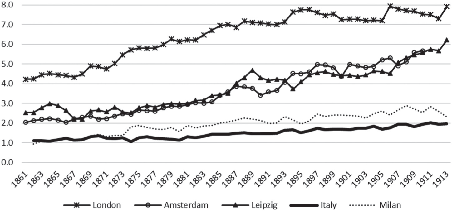
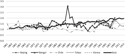
In Figures 1A and 1B, we provide an international comparative perspective of Italian living standards based on 250 working days and the simplified bare bones basket, described in the previous section.Footnote ¹² Figure 1A shows a large gap in WR between Italy and the most developed European countries, here represented by Allen’s estimates for three large cities. Up to the early 1880s, the Italian WR remained around 1.2—that is, an unskilled laborer working full time could earn a little more than what is necessary to support his family at the minimum subsistence level. The WR reached 1.5 for the first time in 1888 and fluctuated around 1.6–1.7 until the early 1900s. Thereafter it started to grow, with some acceleration, but, on the eve of WWI, the WR was still less than 2. As a result, the gap with the most advanced countries, where the WRs considerably increased, had further widened. The WR for Milan shows that the Northern city moved somewhat above the nationwide averages.Footnote ¹³ Italy was quite poor even when compared with other European peripheral countries, such as Austria, and with less developed countries on other continents (Figure 1B).

Figure 1A

WR IN COMPARATIVE PERSPECTIVE: ITALY VERSUS DEVELOPED COUNTRIES

Notes: All data assume 250 working days per year.Sources: Authors’ own elaborations on data kindly provided by Allen previously presented in Allen (2001) and in Allen et al. (2011).

Figure 1B

WR IN COMPARATIVE PERSPECTIVE: ITALY VERSUS LESS DEVELOPED COUNTRIES

Notes: All data assume 250 working days per year. We double the WR for Vienna, because the data refer to a “respectable” basket, which should be worth twice the bare-bones basket according to the Allen method. Actually the basket for Vienna is richer than Allen’s “respectable” one, and, indeed, Cvrcek (2013, footnote 17) warns that his estimates might be slightly undervalued.Sources: Authors’ own elaborations on data from Allen et al. (2011), Cvreck (2013), and Cha (2015).

The Italian WR remained at the same level of most of the countries to the 1880s. Its growth since the 1890s brought it within reach, and in some cases to a higher level of the urban wages in Japan and China. On the eve of WWI, Italy was slightly above the level of all less developed countries of the sample. This result may seem surprising, but this low level of real wages, as well as its upward trend, is consistent with the estimates by Daniele and Malanima (Reference Daniele and Malanima2017).Footnote ¹⁴ Furthermore, our findings are consistent with the available evidence on heights (Federico Reference Delogu2003; Peracchi 2008; A’Hearn and Vecchi 2017; for an international comparison, Baten and Blum (Reference Baten, Blum, van Zanden, Baten and D’Ercole2014)).

The gap between Italy and the advanced countries was much smaller in GDP per capita than in WRs and Italy’s GDP was significantly higher than the Japanese and above all the Chinese measures.Footnote ¹⁵ This difference in Italy’s relative position in terms of GDP and WR can be accounted for by several factors such as a lower labor income share, or higher labor supply per capita, or significant differences in workforce composition in terms of skills, or in the ratio between prices of wage goods and the implicit deflator of GDP (Angeles Reference Angeles2008). Regardless, in spite of the modest improvements in the pre-WWI period, Italian workers remained very poor throughout the entire period between 1861–1913.

REAL WAGES AND THE ITALIAN REGIONAL DIVIDE

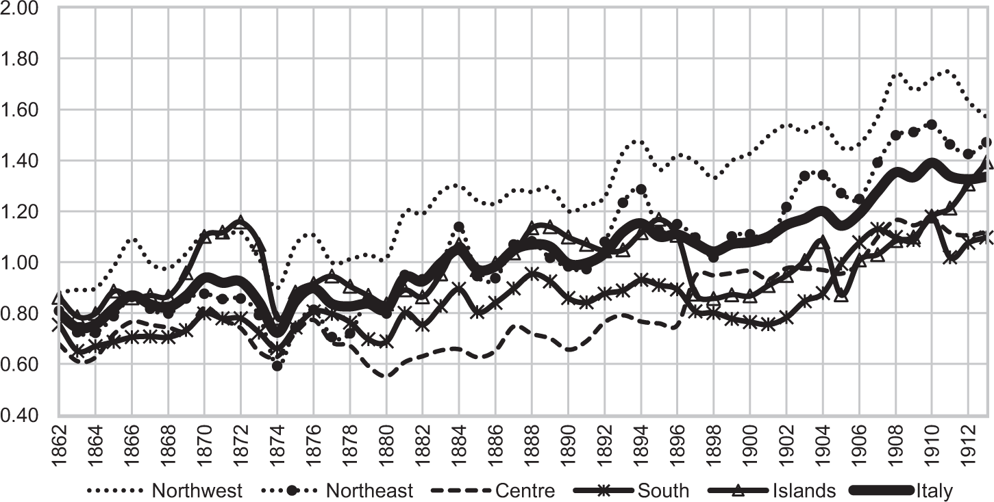
In Figure 2, we present our main estimates of the WRs for the Italian macro-areas. The gap between North (both West and East) and the Continental South was already sizeable at the time of the Unification and real wages remained more or less flat in the following 20 years. Thus, our results seem to be more in line with the conventional wisdom than with the revisionist approach endorsed by Daniele and Malanima (Reference Daniele and Malanima2007, Reference Daniele and Malanima2017). In particular, we do not find any support for the notion of a sudden and drastic impoverishment of the South due to the Unification (Capecelatro and Carlo 1972).

Figure 2

WR FOR UNSKILLED WORKERS

Sources: Authors’ own elaborations (see text and Online Appendix A).

Real wages in the Northwest started to grow from the 1880s, most likely as a consequence of the early industrialization of the “industrial triangle.” The trend accelerated at the turn of the century, peaking in 1910–1911 around 1.75.Footnote ¹⁶ In contrast, in other macro-areas, real wages fluctuated without any clear trend until the first years of the twentieth century. From 1905 to 1913, WR in the Islands increased considerably (59.9 percent), fully recovering after a previous collapse; WR also increased substantially in the Northeast (15.6 percent), the Centre (17.2 percent), and the South (10.3 percent).

The cases of the Islands and Centre deserve some additional comments. The very low WRs in the Centre are consistent with the evidence on incomes for sharecroppers, who accounted for a large majority of the agricultural workforce, in the early twentieth century.Footnote ¹⁷ Sharecroppers received incomes in kind as lodging and they had an implicit right to be subsidized in case of distress. Furthermore, market wages were reduced by the supply of labor from members of sharecropping households moonlighting for causal work. A conceptually similar argument can account for the relatively high level of WR in the Islands, which are higher than those prevailing in the continental South. In this case, as also suggested by Daniele and Malanima (Reference Daniele and Malanima2017), the pattern of settlement of the agricultural workforce in very large agglomerations (“agro-towns”), typical of extensive cultivation, prevented women to seek agricultural employment.Footnote ¹⁸ These low employment rates for women lead to higher wages for man in order to guarantee the survival of the household.Footnote ¹⁹ Indeed, the gender ratio of agricultural workers (female over males) for the Islands according to population censuses was 0.13 in 1871 and declined to 0.11 in 1911, while in the rest of the country it increased from 0.63 to 0.73 (MAIC 1874–1876; Vitali 1968).

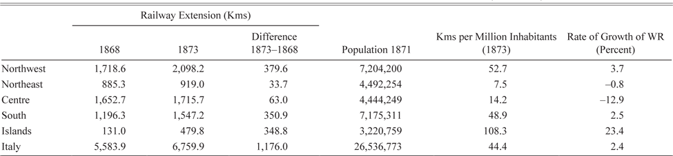
Furthermore, the series for the Islands exhibits a sharp rise in the early 1870s, exceeding in 1872 the level of the Northwest. We interpret this peak as an outcome of the substantial investment in public works, and especially in railways. During the 1860s railway lines were opened for the first time in Sardinia and the Sicilian network was greatly expanded, so that the ratio of new lines per population in the Islands was the highest in Italy in 1868–1873 (Table 3). This resulted in the market for construction workers being very tight (Daniele and Malanima Reference Cvrcek2017). The figure in Table 3 corresponds to about a kilometer of new railways built every 9,200 inhabitants in the Islands, versus a kilometer every 22,600 inhabitants in the whole country (and 133,000 in the Northeast). This can also account for the 17 percent gap between construction and agricultural wages prevailing in 1870 in the Islands (Table 2).

Table 3

THE DEVELOPMENT OF RAILWAY CONSTRUCTIONS BY MACRO-AREAS (1868–1873)

Sources: Ciccarelli and Groote (Reference Cappelli and Vasta2017) for railway lines; population from Population Census (MAIC 1874).

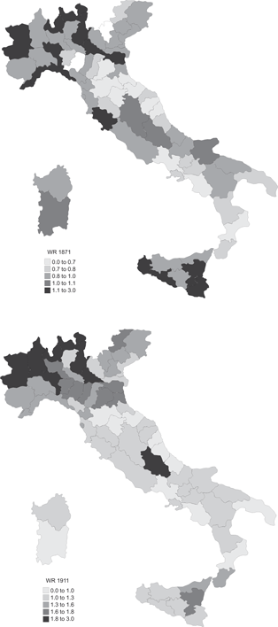
The discussion so far has focused on macro-areas, but, as strongly stressed by several authors (Salvemini 1984; Pezzino 1987; Donzelli Reference Daniele and Malanima1990), there were some dynamic areas within the South, while in the Northwest there were agricultural areas hardly touched by industrialization. We explore differences within macro-areas by mapping WR by province in 1871 (the first year in which Italy had the 1911 borders) and in 1911 (Figure 3).Footnote ²⁰

Figure 3

PROVINCIAL WR FOR 1871 AND 1911

Note: WR are calculated as three years average centered on the year reported in the maps.Source: Authors’ own elaborations.

The provincial maps (Figure 3) show that divergences within regions were still quite significant in the 1871.Footnote ²¹ Most Northwest provinces show comparatively high WRs, but several other provinces, scattered all over the country, also have relatively high levels of WR. By 1911, there is a clear North-South gradient and the provinces with (relatively) high WRs are to be found, exclusively, all over the North. Data show sizeable differences within macro-areas, as appears evident looking at yearly series of WR by region (Figure A1 in Online Appendix A). For instance, the increase in WR from 1905 to 1913 was much more impressive in Sicily (+69 percent) than in Sardinia (+17 percent), while the overall modest growth in the Continental South was determined by wide and largely uncorrelated fluctuations in the underlying provincial WR. In the Northwest, WRs grew fairly steadily in Piedmont and Lombardy, while in Liguria they remained broadly constant, at a rather high level for Italian standards, in the 1860s and 1870s, and boomed in pre-war years. In the long run, the coefficient of variation of regional WRs declined by a couple of points, from 0.212 in 1870–1878 to 0.194 in 1905–1913. Interestingly, the coefficient of variation was stable and also very similar in Austria-Hungary (0.195 in 1870–1878 and 0.198 in 1905–1910) (Cvrcek Reference Ciccarelli and Fachin2013).

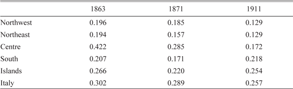
In Table 4, we explore this decline by reporting the population weighted coefficients of variation by macro-area. The coefficient of variation dropped from 0.302 in 1863 to 0.257 in 1911 for Italy (sigma-convergence).Footnote ²² Similar trends are evident in the Centre, in the Northwest and in the Northeast, while there are mixed trends in the South and in the Islands.

Table 4

SIGMA-CONVERGENCE OF WR

Notes: Population weighted coefficients of variation (three years average centered on the year reported in columns).

Source: Authors’ own elaborations.

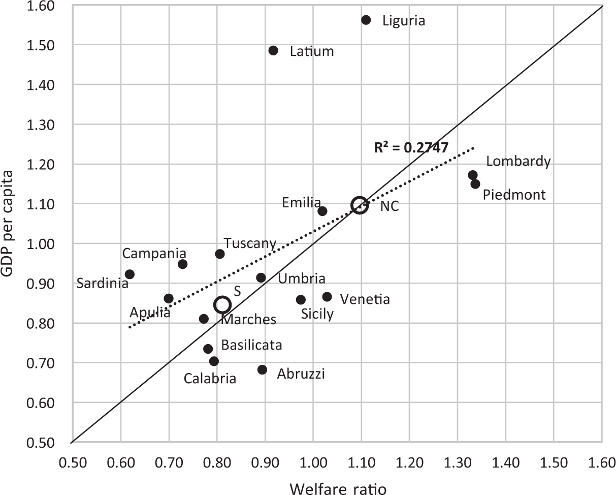
So far we have focused on the WR as proxy for the standard of living of laborers, but real wages are also often used as a proxy for GDP. Figures 4A and 4B show regional GDP per capita and real wages in 1871 and 1911 indexed to the average value of Italy =1. If real wages were a perfect proxy for GDP, all points would be aligned along the 45 degree line. This is clearly not the case. A visual inspection shows some regularities, with few notable changes. In 1871, there were eight regions (Piedmont, Liguria, Abruzzi, Umbria, Basilicata, Calabria, Sardinia, and Sicily) significantly below the 45 degree line, four (Tuscany, Latium, Marches, and Campania) above it, and four regions (Lombardy, Venetia, Emilia, and Apulia) very close to the line. By 1911, only Liguria and Sardinia substantially changed their position.

Figure 4A

GDP PER CAPITA AND WR IN 1871

Figure 4B

GDP PER CAPITA AND WR IN 1911

Sources: Authors’ own elaborations for WR and from Felice (2014) for GDP.

GDP and real wages can differ for a number of factors relating to income distribution, characteristics of labor supply, and relative prices. A comprehensive analysis of the relative contribution of these factors is beyond the scope of this article. However, we can provide a rough glimpse of the role of income distribution by comparing our estimates with the estimates of Gini coefficients for the Centre-North and the South by Nicola Amendola, Andrea Brandolini, and Giovanni Vecchi (Reference Amendola, Brandolini, Vecchi and Vecchi2011, fig. 7.9). The relative position of our WR estimates for these Centre-North and South areas (circles in Figures 4A and 4B) and their movements over time are broadly consistent with these Gini coefficients. Indeed, in 1871, income distribution was more unequal in the North-Centre than in the South. Successively, in 1911, inequality declined in the North-Centre and increased in the South. Needless to say, all inferences for 1871 are speculative given the underlying fragility of the GDP estimate in that year.

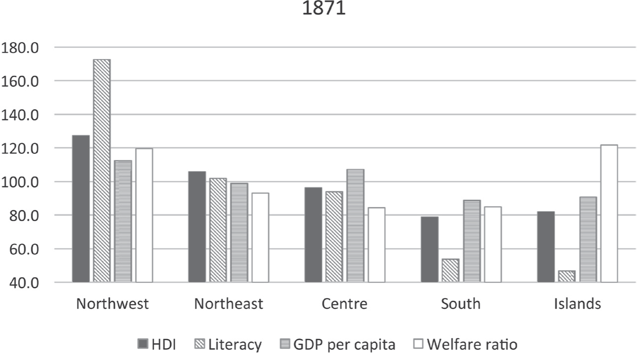
Finally, in Figures 5A and 5B (constructed using histograms with Italy = 100), we compare our WRs for 1871 and 1911 with HDI, as a broader measure of living standards (Felice and Vasta Reference Federico2015), and literacy rates, including also GDP per capita for completeness. Overall, both in 1871 and 1911, there is a broad correlation between HDI and literacy on one side, and WRs on the other side, with the two, previously discussed exceptions, the high wages in the Islands in 1871 and the relatively low wages in the Centre in 1911. Additionally, it is worth noting what is perhaps the most important feature of Figure 5A: namely the extremely high levels of literacy rate already achieved in the Northwest in 1871.Footnote ²³

Figure 5A

MACRO-AREAS INDICATORS, 1871 (ITALY=100)

Figure 5B

MACRO-AREAS INDICATORS, 1911 (ITALY=100)

Sources: Felice and Vasta (2015) for HDI; Population Censuses (MAIC 1874, 1914–1916); Felice (2014) for GDP; and authors’ own elaborations for WR.

CHANGES IN WR: PROXIMATE AND ULTIMATE CAUSES

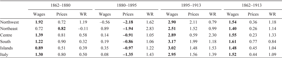
We start our analysis of growth in the WR, by decomposing the overall change in terms of changes between prices and wages. In Table 5, we report the average annual growth rates of WR as the difference between the annual growth of nominal wages and the annual growth of nominal prices.Footnote ²⁴ Figures in bold indicate the prevailing determinant in each macro-areas for three different sub-periods. The results highlight a substantial difference between periods. Over the whole period, and especially during the Giolittian boom (1895–1913), the WR increased from a growth of wages despite price rises. With the notable exception of the Northeast, the rise in wages accounted also for the very modest increase for the period 1862–1880. In contrast, in 1880–1895, the WR rose mostly due to the decline in world prices of cereals, which cut the cost of the bare bones basket in spite of protection on wheat.

Table 5

DECOMPOSITION OF THE GROWTH OF WR (1861–1913)

Notes: Annual yearly growth rates of nominal wages, prices, and WR. Figures in bold indicate the prevailing determinant in each macro-areas for three different sub-periods.

Source: Authors’ own elaborations.

The traditional historiography has interpreted the patterns of Table 5 as driven by two proximate causes: industrialization in the Northwest and emigration for the rest of the country and, in particular, for the rise of wages in the South and in the Islands in the last sub-period (Taylor and Williamson 1997; Hatton and Williamson Reference Hatton and Williamson1998). Alan Taylor and Jeffrey Williamson (Reference Taylor and Williamson1997) argue that emigration was a key factor mitigating Italian GDP divergence relative to the European core in the pre-WWI period.

However, the literature surveyed earlier highlighted five major possible “ultimate” drivers of the growth of real wages: human capital, resource endowments, market potential, infrastructure, and social capital. Here, we provide an appraisal of the relative strength of these factors by using a simple growth regression framework, which allows us also to assess possible trends of convergence as a result of growing integration of labor markets. Ideally, one should have adopted a panel dynamic approach in order to have more precise estimates and to limit possible concerns about endogeneity (Durlauf, Johnson, and Temple Reference Daniele and Malanima2005). Unfortunately, we are constrained to use a long-run specification with co-variates for the initial year (1871), because we lack a full provincial coverage of real wage observations from 1879 to 1904. Accordingly, we estimate the following equation using a provincial cross-section:

(4) $$\eqalign{\widehat{WR}_{1871-1911} = a + b \cdot \ln \left({WR_{1871}}\right) + c \cdot \ln \left({Literacy_{1871}}\right) + d \cdot \\ \ln \left({SocCap_{1871}}\right) + e \cdot \ln \left({MktPot_{1871}}\right) + f \cdot \ln (Rail_{1871} + g \cdot \ln (Water) + \varepsilon,} $$

where, $\widehat{WR}$_1871–1911 is the average compounded growth rate of WR. We have the following co-variates:

1. i. Literacy ₁₈₇₁ is our measure of human capital and it has been retrieved from MAIC (1874);

2. ii. SocCap ₁₈₇₁ is the index of “cooperative norms” constructed by Cappelli (Reference Brunetti, Felice, Vecchi and Vecchi2017), which is computed as the average of donations per capita to Opere Pie (charities) and of the number of mutual aid societies per capita, both relative to the Italian average;

3. iii. MktPot ₁₈₇₁ is the measure of domestic market potential at provincial level constructed by Basile and Ciccarelli (Reference Basile and Carlo2018);

4. iv. Rail ₁₈₇₁ is the kilometers of railway per square kilometer from Ciccarelli and Peter Groote (Reference Ciccarelli and Groote2017);

5. v. Water is our measure of the natural resource endowment. In this context, the literature has mostly emphasized the role of water resources that provided some geographical areas with an enhanced “attractiveness” for industrial activities (A’Hearn and Venables Reference A’Hearn, Venables and Toniolo2013). Following Nuvolari and Vasta (2017), we proxy this factor using the (yearly) flow of rivers, canals, and streams in the province (measured in m3/s). The source of this variable is the website: www.acq.isprambiente.it/pluter/ (see Nuvolari and Vasta (2017) for further details).

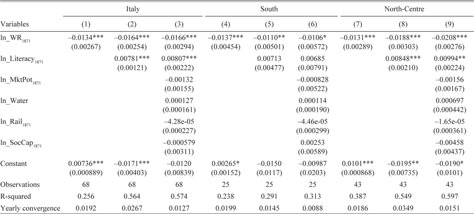
We expect these covariates to exert a positive impact on the growth of WR. Consistently with the standard growth regression exercises, we also include in our specification the initial value of the real wages (WR ₁₈₇₁). The sign of this variable is undetermined a priori: a negative sign will indicate a convergence trend, while a positive sign will indicate divergence. Table 6 reports the results of our regressions. Columns (1)–(3) refer to the entire national sample, Columns (4)–(6) to the Southern provinces, and Columns (7)–(9) to the North and the Centre.

Table 6

GROWTH REGRESSIONS OF WR (1871–1911)

* = Significant at the 10 percent level.

** = Significant at the 5 percent level.

*** = Significant at the 5 percent level.

Note: Robust standard errors in parentheses.

Source: Authors’ own elaborations.

For the whole period we find that the only consistently significant driver is human capital, as proxied by the literacy rate. In particular, this turns out to be significant in the national and in the North-Centre subsample, but, interestingly enough, not in the South. The coefficient for literacy (0.00807) in the most complete national specification (Column 3) implies that moving in 1871 from the province with the lowest literacy rate (Caltanissetta = 8.3 percent) to the province with the highest literacy rate (Turin = 57.7 percent) would lead to an increase of the annual growth rate of real wages of about 1.6 percent.Footnote ²⁵ This is a relatively strong impact since the average of the yearly growth rate of real wages of all provinces in the period 1871–1911 was 0.9 percent. The order of magnitude (2 percent per year) of this impact is similar to the effect of literacy on industrial productivity growth estimated by Cappelli (2017, p. 353) using the same thought-experiment. None of the other variables are significant. However, literacy, market potential, water resources, the railway endowment, and social capital were already higher in the Northwest in 1871 and, thus, they may account for the gap in WRs at the time. Our results suggest that, amongst these variables, only literacy fostered subsequent growth in real wages in the Northwest, offsetting a possible disadvantage of high wages in these regions.Footnote ²⁶

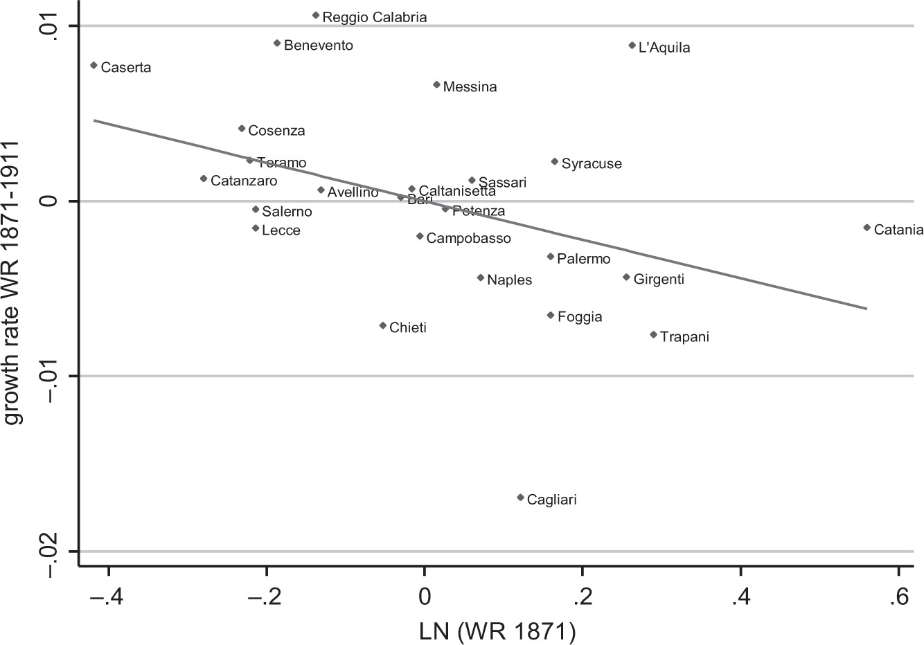
Overall, these effects are consistent with some of the most recent contributions presented earlier. We also find a negative and significant coefficient across all specifications from the initial level of wages. This implied that yearly β convergence rates (Table 6 bottom row) are in line with those found for unskilled urban workers (from 1.8 to 2.8 percent) and somewhat lower of those of agricultural workers (from 3.4 percent to 4 percent) in Spain in the same period (Roses and Sánchez-Alonso Reference Roses and Sánchez-Alonso2004). The results by sub-sample indicate a stronger convergence, in the conditional convergence regressions, in the North-Centre than in the South. This difference is also highlighted by Figures 6A (North-Centre sample) and 6B (South sample), which show partial regressions diagrams of growth rates and initial real wage conditional to the literacy variable (Columns 2, 5, and 8 of Table 6). Overall these different patterns of convergence within macro-areas result in divergence between North-Centre and South, as already shown in the maps of Figure 3, and in the circles in Figures 4A and 4B.

Figure 6A

PARTIAL REGRESSIONS (NORTH-CENTRE SAMPLE)

Figure 6B

PARTIAL REGRESSION (SOUTH SAMPLE)

Notes: The figure plots the average annual growth rate of WR against the level of WR in 1871 after controlling for the literacy level in 1871.Source: Authors’ own elaborations.

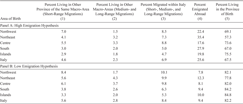
We interpret this convergence profile as an outcome of short-range domestic migration and we buttress this view with the data shown in Table 7. In Table 7, we compute total migration according to two different hypotheses: (i) a “high emigration hypothesis,” which refers to gross migration for the period 1876–1911 (Table 7, Panel A), and (ii) a “low emigration hypothesis,” which includes only net (gross less returns for the 1905–1911 period only) migrations (Table 7, Panel B). The former is clearly an upper bound, as it includes emigrants who returned home before 1911 (possibly with repeated rounds of migration) or who died abroad, while the latter is a lower bound since data on net migration are available only for a limited period of time. Mass migration started in the 1880s, but the data before 1904 refer only to gross flows, even though a substantial number of Italians returned home (and were, thus, counted in the 1911 census).Footnote ²⁷ In particular, we compute the percentage of Italians living outside the province of birth in 1911 as the sum of people living in another province of the same macro-area (short-range migrations, Table 7, Column 1) and in another macro-area (medium- and long-range migrations, Column 2), as registered by the 1911 Census (MAIC 1914–1916). Thus, Column 3, the sum of Columns 1 and 2, is the percentage of people who migrated within Italy. In contrast, people emigrated abroad are presented in Column 4. Finally, we obtained as residual Column 5, the percentages of people that, in 1911, lived in the same province of birth.

Table 7

PEOPLE RESIDENT IN 1911 BY PLACE OF BIRTH

Sources: For domestic migrations: MAIC (1914–1916); for international migrations: ISTAT, Statistiche storiche on line (http://seriestoriche.istat.it, last access July 2017).

Table 7 highlights two main points: first, short-range migrations were considerably greater within the Northwest than within any other macro-areas, and, second, many more Southerners moved abroad than to other provinces. The census data for 1911 reveal two other important features of the migrations process, not reported here for space constraints. First, about two-thirds of the people born in the Northeast, and living in another macro-area, were actually residents in the Northwest. Second, in 1911, about 15 percent of the inhabitants of the Northwest were born outside the province of residence. In a nutshell, we observe a dual movement: the early development of an Italian sub-national labor market in the industrializing Northwest (Federico Reference Federico1985), with some attraction also from the neighboring macro-areas, and a massive integration of the South (but also of the Northeast) with the transatlantic labor market (Hatton and Williamson Reference Hatton and Williamson1998; Gomellini and Ó Gráda Reference Gomellini, Ó Gráda and Toniolo2013).Footnote ²⁸ Overall, this interpretation is consistent with the existence of sigma-convergence in the North and in the Centre and of (modest) sigma-divergence in the South and Islands (possibly due to different rates of foreign migrations across provinces in the South) as shown in Table 4.