1 Introduction
The search for organised motion in high Reynolds number turbulent flows has been an important object of study since the 1960s. The identification of order in flows previously considered to be entirely stochastic has broken old paradigms and established new ways of analysing turbulence. Study of the turbulent jet led to the discovery of axially extended, organised waves with amplitude modulation, referred to in the literature as wavepackets. Despite their low energy, such structures are found to be a central element of the jet dynamics, with amplitude growth related to the Kelvin–Helmholtz instability mechanism, and are important for sound generation on account of their spatio-temporal coherence (Mollo-Christensen Reference Mollo-Christensen1967; Crow & Champagne Reference Crow and Champagne1971; Crighton Reference Crighton1975; Cavalieri et al. Reference Cavalieri, Rodríguez, Jordan, Colonius and Gervais2013; Jordan & Colonius Reference Jordan and Colonius2013; Breakey et al. Reference Breakey, Jordan, Cavalieri, Nogueira, Léon, Colonius and Rodríguez2017). In supersonic jets wavepackets generate sound through Mach-wave radiation (Tam & Burton Reference Tam and Burton1984; Sinha et al. Reference Sinha, Rodríguez, Brès and Colonius2014), but in subsonic jets sound radiation is associated with wavepacket jitter (Cavalieri et al. Reference Cavalieri, Jordan, Agarwal and Gervais2011; Cavalieri & Agarwal Reference Cavalieri and Agarwal2014), which is postulated to be due to the interaction of wavepackets of low amplitude and azimuthal wavenumber with the energy-containing eddies of the turbulent field.
In wall-bounded flows, orderly structures have also been an object of study for some time, and in particular those characterised by streamwise vortices coupled with elongated streaks. Several such studies have been performed for boundary layers. Kline et al. (Reference Kline, Reynolds, Schraub and Runstadler1967) identified organised streaky structures in the viscous sub-layer of boundary layers, with dynamics corresponding to a lift-up mechanism. Later, Smith & Metzler (Reference Smith and Metzler1983) explored some characteristics of these streaks, finding their spacing to be invariant with Reynolds number; the spanwise spacing is
 $\unicode[STIX]{x1D706}_{z}^{+}=100$
for wall distances
 $y^{+}<5$
; here, the
 $+$
superscript indicates non-dimensional distances with respect to the friction velocity and the kinematic viscosity. Streaks located in the upper regions of the boundary layer (
 $y^{+}>10$
) have increasing spacing as the Reynolds number
 $Re$
is increased. The cited works motivated several research directions, especially concerning regions of the boundary layer responsible for turbulent kinetic energy production, and the role of streaks in this process (Smits, McKeon & Marusic Reference Smits, McKeon and Marusic2011). More recently, Hutchins & Marusic (Reference Hutchins and Marusic2007) performed particle image velocimetry (PIV) and hot-wire experiments and compared their results with those of a model, showing that the meandering motion of streaks can mask their real length: single-point statistics may lead to results that do not correspond to the reality. In their analysis, Hutchins and Marusic found very large streaky structures in the logarithmic region of high Reynolds number boundary layers, with streamwise extent larger than 20 times the boundary layer thickness; these were labelled as superstructures. Similar structures have also been found in turbulent channel and pipe flows by Monty et al. (Reference Monty, Stewart, Williams and Chong2007).
The role of streaks and streamwise vortices in turbulence dynamics has been extensively studied for wall-bounded flows. Seminal work by Ellingsen & Palm (Reference Ellingsen and Palm1975) (later completed by Landahl (Reference Landahl1980)) considered the stability of linearly sheared flow, reaching the conclusion that, though the flow may not support exponential growth of disturbances (in the modal linear stability analysis framework), there may nonetheless be significant disturbance amplification via a non-modal, linear mechanism. Spanwise-periodic, streamwise independent vortices have wall-normal velocity components that transfer fluid across a sheared base flow, lifting fluid from low- to high-speed regions (leading to a streak of low streamwise velocity) and from high- to low-speed regions (with a consequent high-speed streak). This creates a large amplification of the streamwise velocity, forming spanwise-periodic streaks, in what is referred to as the lift-up effect. This phenomenon was identified not only in Couette flow, but in other canonical wall-bounded flows such as plane Poiseuille flow (Gustavsson Reference Gustavsson1991) and boundary layers (Hultgren & Gustavsson Reference Hultgren and Gustavsson1981). The main signature of this effect is the presence of streamwise elongated structures in the near-wall region of the turbulent flow. Work by Hamilton, Kim & Waleffe (Reference Hamilton, Kim and Waleffe1995) and Waleffe (Reference Waleffe1995), later developed by Schoppa & Hussain (Reference Schoppa and Hussain2002) and Farrell & Ioannou (Reference Farrell and Ioannou2012), shows that these structures (streaks and streamwise vortices) are an intrinsic part of the dynamics of a wall-bounded turbulent shear flow, and constitute two of the building blocks that characterise the self-sustaining nature of turbulence. As summarised by Waleffe (Reference Waleffe1995), this process would consist of three main components: first, the occurrence of (i) a spanwise modulation of the streamwise velocity by streamwise vortices, which generates streaks; followed by (ii) a breakdown of the streaks by an inflectional wavelike instability; finally, (iii) the streamwise vortices are regenerated by a nonlinear self-interaction of the streak instability, restarting the process.
All of the studies discussed above consider wall-bounded shear flows. There are few studies of similar structures for unbounded, free-shear flows, such as shear layers and round jets. Bernal & Roshko (Reference Bernal and Roshko1986) performed flow visualisation in water using a schlieren technique in two perpendicular sections of a plane mixing layer, revealing the presence of Kelvin–Helmholtz vortices and streamwise streaks; such structures were generated in the upstream region of the flow and sufficiently amplified in the downstream region to be visible in the photographs. Later, Liepmann & Gharib (Reference Liepmann and Gharib1992) found similar structures in a transitional round jet of low Reynolds number (
 $Re=5500$
, based on the jet diameter) using particle image velocimetry (PIV) measurements. Their analysis concluded that streamwise vortices have a vital effect on the entrainment rate and on the dynamics of the shear flow, which agrees with wall-turbulence research, as stressed by Kozlov et al. (Reference Kozlov, Grek, Lofdahl, Chernorai and Litvinenko2002). Similarly, Jung, Gamard & George (Reference Jung, Gamard and George2004) used 138 hot-wires to analyse the radial structure of the most energetic modes in a low Mach number
 $(M)$
jet, performing a slice-by-slice proper orthogonal decomposition at various axial stations. This was later complemented by the analysis of Tinney, Glauser & Ukeiley (Reference Tinney, Glauser and Ukeiley2008), who performed PIV measurements for a
 $M=0.85$
jet. In both studies, the authors found that the most energetic structures peak at non-zero azimuthal wavenumbers, with decreasing values of the peak wavenumber as the PIV plane or the hot-wire device was moved downstream. However, no clear association of such structure with the lift-up mechanism in wall-bounded flows was made, and a characterisation of the streamwise extent of these structures was still lacking.
Interest in the role played by streaks in free-shear flows has increased in recent years. Jiménez-González & Brancher (Reference Jiménez-González and Brancher2017) studied the problem of the disturbances that experience the largest temporal transient growth in round jets, studying both static and diffusing base flows. The optimal initial disturbance was found to take the shape of streamwise vortices, leading to amplified streaks, with gains that scale with
 $Re^{2}$
regardless of the diffusive nature of the base flow. Moreover, the different azimuthal modes
 $m$
appear to be underpinned by different mechanisms: while
 $m\geqslant 2$
appears to be related to the lift-up mechanism (with growth rates that scale with
 $1/m^{3}$
),
 $m=1$
disturbances are more related to a shift-up mechanism, a dynamics that shifts the entire jet in the radial direction. Finally, Marant & Cossu (Reference Marant and Cossu2018) evaluated optimal transient growth in a hyperbolic–tangent mixing layer, reaching similar conclusions as Jiménez-González & Brancher (Reference Jiménez-González and Brancher2017): the growth rate scales with
 $Re^{2}$
and the optimal initial disturbances consist of streamwise vortices, which give rise to streamwise streaks as they evolve in time. They also analysed how streaks can change the characteristics of the Kelvin–Helmholtz instability, finding both stabilising and destabilising effects depending on whether optimal sinuous or suboptimal varicose mode are considered in the analysis. Both studies are theoretical, and to date conclusive evidence of the presence of large-scale streaks in free turbulent shear flow is lacking. An identification of such structures would be of considerable interest, since their effect on Kelvin–Helmholtz wavepackets may aid in the modelling of turbulent jet noise.
The main objective of this paper is to show that streaky structures can also be found in unbounded, free-shear flows of high Reynolds number using the same tools used in wall-bounded turbulence, such as proper orthogonal decomposition, spatial Fourier transforms, resolvent and transient growth analyses. We analyse a
 $M=0.4$
jet using PIV measurements and the cited methods. Results show a high resemblance to what is found for turbulent pipe flow and boundary layers, supporting the hypothesis that this structure is a fundamental component of turbulence dynamics, not only in wall-bounded flows, but in any shear flow.
The remainder of the paper is organised as follows. In § 2 we present the experimental set-up. In § 3 we describe the spectral proper orthogonal decomposition (SPOD), resolvent and transient growth analysis frameworks. Afterwards, in § 4 we present the main results from the study, starting with a Fourier transform analysis, followed by the SPOD results and a comparison with the equivalent cases from resolvent and transient growth analyses. The paper is closed with a summary of the conclusions in § 5.
2 Experimental set-up
The present work uses the experimental database reported in Jaunet, Jordan & Cavalieri (Reference Jaunet, Jordan and Cavalieri2017). All experiments were conducted at the ‘Bruit et Vent’ jet-noise facility of the Pprime Institute, Poitiers, France. The Mach number chosen for the analysis was
 $M=0.4$
and the nozzle diameter
 $D=0.05~\text{m}$
, leading to a diameter-based Reynolds number of
 $Re=4.6\times 10^{5}$
; the corresponding momentum-thickness-based Reynolds number
 $Re_{\unicode[STIX]{x1D703}}$
is
 $4\times 10^{3}$
. The settling chamber contains a series of honeycombs structures and grids to remove residual turbulence in the potential flow field. The flow is then accelerated into a convergent–straight nozzle, where the boundary layer is tripped to ensure transition to turbulence upstream the nozzle exit. Velocity measurements inside the nozzle confirm that the boundary layer is turbulent. Details on the exit flow condition can be found in Cavalieri et al. (Reference Cavalieri, Rodríguez, Jordan, Colonius and Gervais2013) and Jaunet et al. (Reference Jaunet, Jordan and Cavalieri2017).
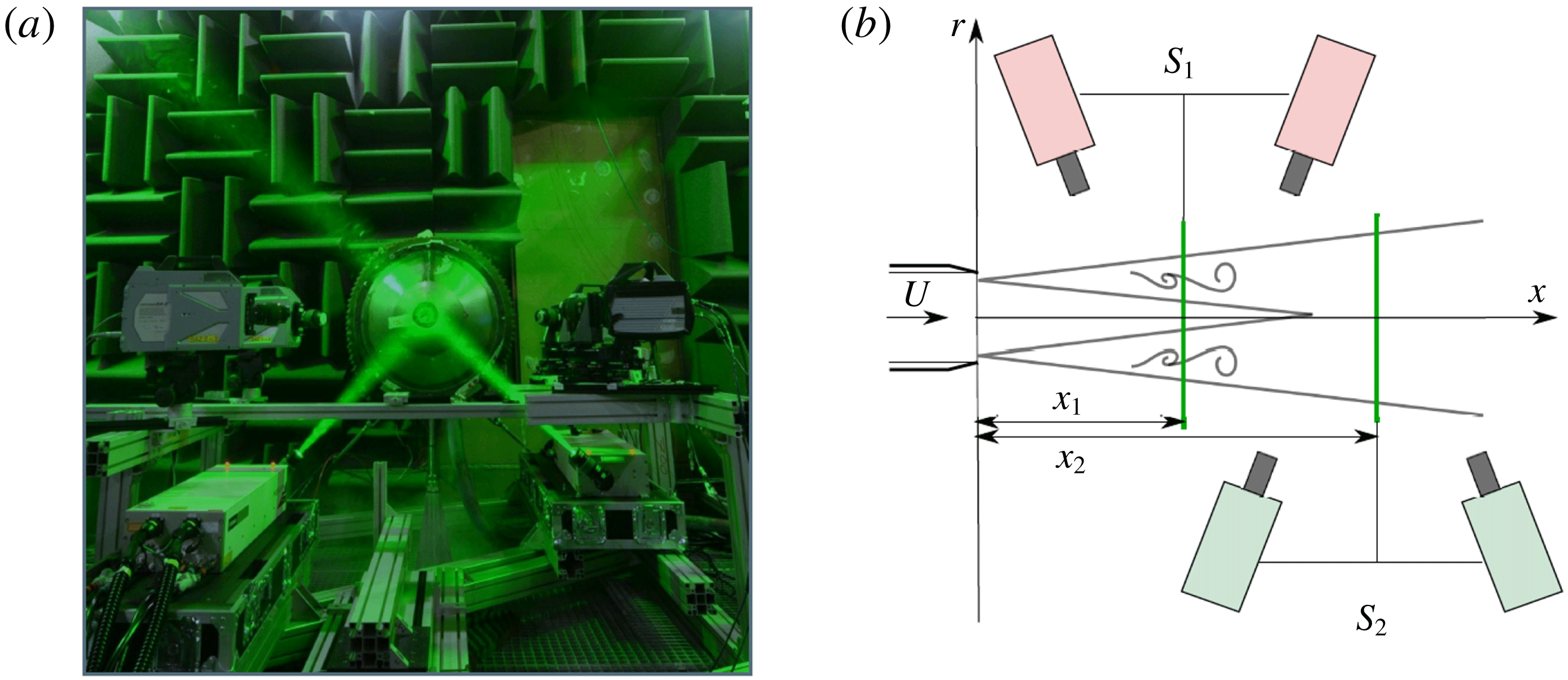
Experimental set-up (a) and coordinate system adopted in the PIV planes (b). Taken from Jaunet et al. (Reference Jaunet, Jordan and Cavalieri2017).
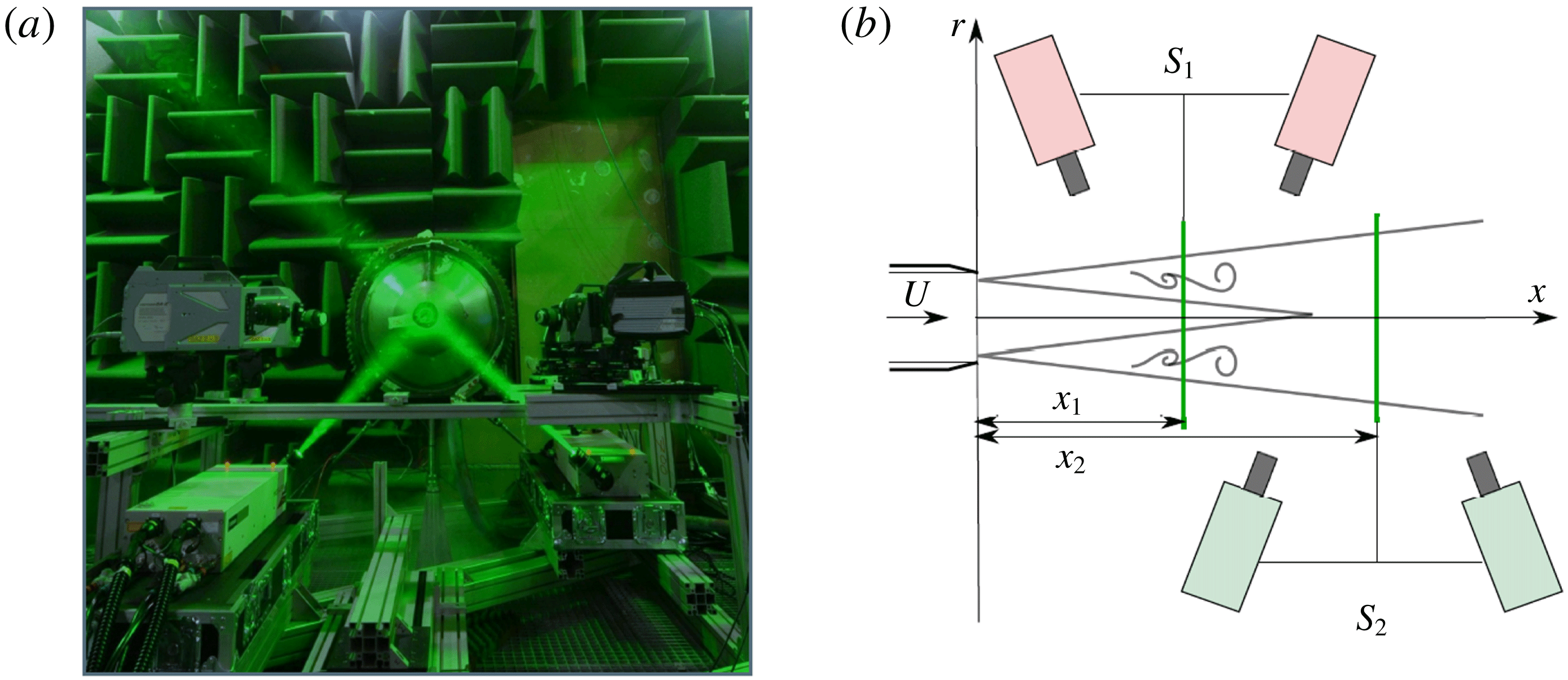
In order to decompose the field into azimuthal Fourier modes and build the cross-spectral matrix, two time-resolved, stereoscopic particle image velocimetry (PIV) systems were used, which could be moved independently, as illustrated in figure 1. The acquisition frequency of the systems was 5 kHz (10 kHz for each PIV system), leading to a sampling interval of
 $\unicode[STIX]{x0394}tU_{jet}/D=0.548$
, where
 $U_{jet}$
is the jet velocity. A total of 19 414 image pairs was recorded for each acquisition point
 $(x_{1};x_{2})$
. The axial positions
 $x_{1}$
and
 $x_{2}$
of the PIV planes varied between
 $1D\leqslant x_{1}\leqslant 8D$
and
 $x_{1}<x_{2}\leqslant 8D$
with a spacing of
 $\unicode[STIX]{x0394}x=0.5D$
; for each position, the first PIV system was kept fixed, while the second was moved downstream until it reached the end of the domain.
Both the jet flow and the surrounding air were seeded by injection of pure glycerine smoke particles in the pipe, upstream of the settling chamber. This ensures a homogeneous seeding with particles having diameters in the range of
 $1{-}2~\unicode[STIX]{x03BC}\text{m}$
, responding at frequencies up to
 $St=fD/U_{jet}=20$
, hence sufficiently small to follow the velocity fluctuations of interest in this study. The particle image velocimetry calculations were carried out using a multipass iterative PIV algorithm (Scarano Reference Scarano2001). The first pass interrogation window size was set to
 $32~\text{pixel}\times 32~\text{pixel}$
and decreased to
 $16~\text{pixel}\times 16~\text{pixel}$
with an overlap of 50 %. This led to a resolution of one vector every 0.85 mm and PIV vector fields containing
 $140\times 110$
velocity vectors. Outliers were detected using the universal outlier detection technique on
 $3\times 3$
interrogation grids. We used a residual threshold of 2, above which vectors were considered spurious (Westerweel & Scarano Reference Westerweel and Scarano2005). Unexpectedly, no sign of peak locking was observed in the data. It is believed that this is due to the fact that the particle images were dewarped (i.e. interpolated) prior to computation of the cross-correlation. This has a blurring effect on the particle images which confines the peak-locking effects beneath the PIV noise floor. In order to perform Fourier transform in the azimuthal direction, the instantaneous velocity fields were interpolated onto a polar grid of 32 points in the radial direction and 64 in azimuth for
 $r/D\leqslant 0.8$
using a bicubic interpolation. The spatial resolution of the interpolated field has been chosen to match the original one in order to avoid any loss of information. More details can be found in Jaunet et al. (Reference Jaunet, Jordan and Cavalieri2017).
In the following, we perform an analysis of the cross-spectral density (CSD) matrix of the PIV data. The CSD is obtained using the Welch periodogram technique with blocks of
 $n_{fft}=128$
samples, with overlap of 50 %. The minimum resolved frequency, and therefore the frequency resolution of the spectral content, is
 $\unicode[STIX]{x0394}St=0.015$
. A standard Hann tapering window was applied to all blocks of data to minimise spectral leakage.
3 Analysis and modelling methods
The analysis and modelling methods employed are described in this section. These involve spectral proper orthogonal decomposition, resolvent analysis and transient growth analysis.
3.1 Spectral proper orthogonal decomposition
The experiment as it was performed allows us to build a cross-spectral matrix for the streamwise velocity component. The data are decomposed into mean and fluctuating components,
 $$\begin{eqnarray}\tilde{u} (\boldsymbol{x},t)=U(\boldsymbol{x},r)+u^{\prime }(\boldsymbol{x},t),\end{eqnarray}$$
where
 $\boldsymbol{x}=(x,r,\unicode[STIX]{x1D703})$
, with the mean taken in time. The fluctuations are then Fourier transformed in time and in azimuth so that
 $$\begin{eqnarray}u^{\prime }(\boldsymbol{x},t)=\int _{\unicode[STIX]{x1D714}}\mathop{\sum }_{m}u(x,r,m,\unicode[STIX]{x1D714})\text{e}^{\text{i}m\unicode[STIX]{x1D703}}\text{e}^{-\text{i}\unicode[STIX]{x1D714}t}\,\text{d}\unicode[STIX]{x1D714},\end{eqnarray}$$
where
 $m$
is the azimuthal wavenumber and
 $\unicode[STIX]{x1D714}$
is the frequency.
Spectral proper orthogonal decomposition (SPOD) is used to identify the most energetic coherent structures. Following Jung et al. (Reference Jung, Gamard and George2004) and Cavalieri et al. (Reference Cavalieri, Rodríguez, Jordan, Colonius and Gervais2013), we can write the SPOD integral equation as
 $$\begin{eqnarray}\int _{\unicode[STIX]{x1D6FA}}\unicode[STIX]{x1D64D}(x,x^{\prime },r,r^{\prime },m,\unicode[STIX]{x1D714})\unicode[STIX]{x1D709}(x^{\prime },r^{\prime },m,\unicode[STIX]{x1D714})r^{\prime }\,\text{d}r^{\prime }\,\text{d}x^{\prime }=\unicode[STIX]{x1D70E}(m,\unicode[STIX]{x1D714})\unicode[STIX]{x1D709}(x,r,m,\unicode[STIX]{x1D714}),\end{eqnarray}$$
where
 $\unicode[STIX]{x1D64D}$
is the two-point cross-spectral tensor of the streamwise velocity fluctuations,
 $\unicode[STIX]{x1D70E}$
is the eigenvalue and
 $\unicode[STIX]{x1D709}$
is the corresponding eigenfunction. The integral is evaluated in the whole experimental domain
 $\unicode[STIX]{x1D6FA}$
.
The eigenvalue problem of (3.3) leads to real, positive eigenvalues
 $\unicode[STIX]{x1D70E}$
and orthonormal eigenfunctions
 $\unicode[STIX]{x1D709}$
. The expression as written in (3.3) relates structures extended over the whole domain, given by the eigenfunctions
 $\unicode[STIX]{x1D709}$
, with their respective energies
 $\unicode[STIX]{x1D70E}$
, allowing us to find the most energetic structures for each
 $m{-}\unicode[STIX]{x1D714}$
pair. The dual PIV configuration used in the experiments only allowed accurate measurement of the streamwise component
 $u$
; thus, the energy represented by the SPOD modes refers solely to the
 $u$
component. Compared to previous works (Jung et al.
Reference Jung, Gamard and George2004; Tinney et al.
Reference Tinney, Glauser and Ukeiley2008; Cavalieri et al.
Reference Cavalieri, Rodríguez, Jordan, Colonius and Gervais2013), which applied POD separately for a number of jet slices, the present spectral POD modes are defined over the entire domain, thanks to the use of two time-resolved PIV planes to obtain the azimuthally resolved cross-spectral density.
3.2 Resolvent analysis
Resolvent analysis has been widely used in several kinds of flow, and is a useful tool to analyse both laminar (focusing on identifying mechanisms of transition) and turbulent flows, which is the present case. We follow the approach described by McKeon & Sharma (Reference McKeon and Sharma2010), using the resolvent to identify optimal response structures in the jet and the shape of the associated optimal forcing. In a locally parallel framework, we consider Fourier transformed variables in the streamwise direction in addition to the Fourier series in azimuthal wavenumber
 $m$
and use the mean flow
 $U(x_{1},r)$
at a given
 $x_{1}$
station as base flow. The linearised Navier–Stokes equations in the input–output form can be written as:
 $$\begin{eqnarray}\displaystyle & \displaystyle \frac{\unicode[STIX]{x2202}}{\unicode[STIX]{x2202}t}\left(\unicode[STIX]{x1D643}\left[\begin{array}{@{}c@{}}\unicode[STIX]{x1D753}\\ p\end{array}\right]\right)(k_{x},r,m,t)=\unicode[STIX]{x1D647}\left[\begin{array}{@{}c@{}}\unicode[STIX]{x1D753}\\ p\end{array}\right](k_{x},r,m,t)+\left[\begin{array}{@{}c@{}}\boldsymbol{f}\\ 0\end{array}\right](k_{x},r,m,t), & \displaystyle\end{eqnarray}$$
 $$\begin{eqnarray}\displaystyle & \displaystyle \unicode[STIX]{x1D753}_{u}(k_{x},r,m,t)=\unicode[STIX]{x1D63E}\left[\begin{array}{@{}c@{}}\unicode[STIX]{x1D753}\\ p\end{array}\right](k_{x},r,m,t), & \displaystyle\end{eqnarray}$$
where
 $\unicode[STIX]{x1D753}=[u\;v\;w]^{\text{T}}$
contains the velocity components (streamwise, radial and azimuthal, respectively) and
 $\boldsymbol{f}=[f_{x}\;f_{r}\;f_{\unicode[STIX]{x1D703}}]^{\text{T}}$
is a forcing term (which is considered to gather the nonlinear terms in the momentum equation); the continuity equation is linear and thus has no forcing term. The matrix
 $\unicode[STIX]{x1D647}$
defines the evolution of the disturbances and
 $\unicode[STIX]{x1D63E}$
is a filter matrix that isolates only the streamwise component of the velocity in the vector
 $\unicode[STIX]{x1D753}_{u}=[u\;0\;0]^{\text{T}}$
for consistency with the SPOD results, which account only for the amplitude of the streamwise component; however, nearly no difference is found in the results if all velocity components are considered in the analysis, since the flow response is dominated by the streamwise component. All the matrix operators are described in appendix A. The radial discretisation is done using Chebyshev polynomials in
 $r$
, following Trefethen (Reference Trefethen2000), and in order to diminish the computational cost, we adopt the same mapping of the radial domain used by Lesshafft & Huerre (Reference Lesshafft and Huerre2007) to concentrate Chebyshev nodes at the shear layer and potential core of the jet; boundary conditions for the azimuthal wavenumbers were implemented in the same fashion as the cited work. The base flow was chosen to be a slice of the experimental mean flow
 $U(x_{1},r)$
at
 $x_{1}/D=2$
, but the choice of other streamwise stations
 $x_{1}$
was seen to lead to similar results. If the linear operator
 $\unicode[STIX]{x1D647}$
is stable one can define a frequency response function between input and output. Assuming Fourier-transformed variables in time, as in (3.2), one can write
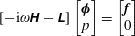 $$\begin{eqnarray}\displaystyle & \displaystyle [-\text{i}\unicode[STIX]{x1D714}\unicode[STIX]{x1D643}-\unicode[STIX]{x1D647}]\left[\begin{array}{@{}c@{}}\unicode[STIX]{x1D753}\\ p\end{array}\right]=\left[\begin{array}{@{}c@{}}\boldsymbol{f}\\ 0\end{array}\right] & \displaystyle\end{eqnarray}$$
 $$\begin{eqnarray}\displaystyle & \displaystyle \Rightarrow \quad \left[\begin{array}{@{}c@{}}\unicode[STIX]{x1D753}\\ p\end{array}\right]=[-\text{i}\unicode[STIX]{x1D714}\unicode[STIX]{x1D643}-\unicode[STIX]{x1D647}]^{-1}\left[\begin{array}{@{}c@{}}\boldsymbol{f}\\ 0\end{array}\right]. & \displaystyle\end{eqnarray}$$
Adopting a compact form for the forcing term via the matrix operator
 $\unicode[STIX]{x1D63D}$
, shown in appendix A, the previous equation leads us to
 $$\begin{eqnarray}\unicode[STIX]{x1D753}_{u}=\unicode[STIX]{x1D63E}[-\text{i}\unicode[STIX]{x1D714}\unicode[STIX]{x1D643}-\unicode[STIX]{x1D647}]^{-1}\unicode[STIX]{x1D63D}\boldsymbol{f}={\mathcal{R}}\boldsymbol{f},\end{eqnarray}$$
where the resolvent operator is given by
 ${\mathcal{R}}=\unicode[STIX]{x1D63E}(-\text{i}\unicode[STIX]{x1D714}\unicode[STIX]{x1D643}-\unicode[STIX]{x1D647})^{-1}\unicode[STIX]{x1D63D}$
. Finding the optimal forcing and associated response of the problem involves solving the following problem:
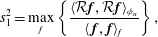 $$\begin{eqnarray}s_{1}^{2}=\max _{f}\left\{\frac{\langle {\mathcal{R}}\boldsymbol{f},{\mathcal{R}}\boldsymbol{f}\rangle _{\unicode[STIX]{x1D719}_{u}}}{\langle \,\boldsymbol{f},\boldsymbol{f}\rangle _{f}}\right\},\end{eqnarray}$$
which can be achieved by performing a singular value decomposition of the operator
 ${\mathcal{R}}$
. Usually, the inner products chosen in (3.9) are defined according to energy norms for input
 $\boldsymbol{f}$
and output
 $\unicode[STIX]{x1D753}_{u}$
. In the present work we choose a norm
 $\langle \cdot ,\cdot \rangle _{\unicode[STIX]{x1D719}_{u}}$
that weights the problem so as to localise responses inside (
 $r/D<1$
) in order to avoid free-stream modes, as reported by Dergham, Sipp & Robinet (Reference Dergham, Sipp and Robinet2013); using that formulation, we perform the analysis for a weighted resolvent operator, isolating the optimals and suboptimals for each frequency and wavenumber leading to amplified responses in the jet region. The weighting function
 $\boldsymbol{W}_{\unicode[STIX]{x1D719}_{u}}$
is given as
 $$\begin{eqnarray}\boldsymbol{W}_{\unicode[STIX]{x1D719}_{u}}=\text{diag}[0.5(1-b)(1+\tanh (r_{p}/D-r/D))+b]\boldsymbol{W}_{cheb},\end{eqnarray}$$
where
 $b$
is a small parameter used to avoid singularities in the matrix inversion and other problems with the Cholesky factorisation;
 $r_{p}/D=1$
is the position where the function goes from 1 to 0, and
 $\boldsymbol{W}_{cheb}$
are the standard quadrature weights for Chebyshev polynomials. With this choice of parameters, we can avoid modes related to the excitation of free-stream disturbances and focus on the structures close to the shear region of the jet. The inner products in (3.9) become, in matrix form,
 $\langle {\mathcal{R}}\boldsymbol{f},{\mathcal{R}}\boldsymbol{f}\rangle _{\unicode[STIX]{x1D719}_{u}}=\boldsymbol{f}^{H}{\mathcal{R}}^{H}\boldsymbol{W}_{\unicode[STIX]{x1D719}_{u}}{\mathcal{R}}\boldsymbol{f}$
and
 $\langle \boldsymbol{f},\boldsymbol{f}\rangle _{f}=\boldsymbol{f}^{H}\boldsymbol{W}_{f}\boldsymbol{f}$
, and the resolvent modes are obtained by taking the singular value decomposition of
 $\boldsymbol{W}_{\unicode[STIX]{x1D719}_{u}}^{1/2}{\mathcal{R}}\boldsymbol{W}_{f}^{1/2}$
, as in Tissot et al. (Reference Tissot, Zhang, Lajús, Cavalieri and Jordan2017) and Towne, Schmidt & Colonius (Reference Towne, Schmidt and Colonius2018). For the present problem, we choose
 $\boldsymbol{W}_{f}=\boldsymbol{W}_{cheb}$
.
With the defined formulation, the output of the resolvent analysis is the optimal forcing that would maximise streamwise velocity in regions where the turbulence intensity is higher (
 $r/D<1$
). The most amplified response corresponds to turbulent structures most likely to be excited by nonlinear dynamics (Cavalieri, Jordan & Lesshafft Reference Cavalieri, Jordan and Lesshafft2019). Moreover, if nonlinear terms in the Navier–Stokes system are modelled as white noise, the resulting SPOD modes should be equal to response modes from resolvent analysis (Towne et al.
Reference Towne, Schmidt and Colonius2018). Resolvent analysis has been previously shown to accurately model wavepackets in turbulent jets, with good agreement between response and SPOD modes for moderate and high Strouhal numbers dominated by the Kelvin–Helmholtz instability (Schmidt et al.
Reference Schmidt, Towne, Rigas, Colonius and Brès2018; Lesshafft et al.
Reference Lesshafft, Semeraro, Jaunet, Cavalieri and Jordan2019), also providing insight into the overall shape of the forcing term. The present study extends the analysis for the low-frequency range, focusing on streaks.
3.3 Transient growth
While the resolvent analysis obtains the harmonic forcing that generates the maximum response, transient growth shifts the analysis to the time domain. It focuses on finding the initial disturbance that will experience the largest growth in time, in a linear non-modal mechanism. Studies like Butler & Farrell (Reference Butler and Farrell1992), Hanifi, Schmid & Henningson (Reference Hanifi, Schmid and Henningson1996), Del Alamo & Jimenez (Reference Del Alamo and Jimenez2006), Cossu, Pujals & Depardon (Reference Cossu, Pujals and Depardon2009) and Pujals et al. (Reference Pujals, García-Villalba, Cossu and Depardon2009) highlight the importance of such analysis for both laminar and turbulent flows. Indications of the optimal paths for transition to turbulence and even the optimal structures present in turbulent flows can be found, and the latter is the focus of the present work (with optimal meaning the structures related to the maximum amplification, which are thus more likely to be found in the experimental data). Considering the problem without forcing (i.e. neglecting nonlinear terms), we can write the evolution of disturbances in the flow as:
 $$\begin{eqnarray}\frac{\unicode[STIX]{x2202}}{\unicode[STIX]{x2202}t}\left(\unicode[STIX]{x1D643}\left[\begin{array}{@{}c@{}}\unicode[STIX]{x1D753}\\ p\end{array}\right]\right)(k_{x},r,m,t)=\unicode[STIX]{x1D647}\left[\begin{array}{@{}c@{}}\unicode[STIX]{x1D753}\\ p\end{array}\right](k_{x},r,m,t),\end{eqnarray}$$
an initial value problem with the solution
 $$\begin{eqnarray}\left[\begin{array}{@{}c@{}}\unicode[STIX]{x1D753}\\ p\end{array}\right](k_{x},r,m,t)=\text{e}^{\unicode[STIX]{x1D647}t}\left[\begin{array}{@{}c@{}}\unicode[STIX]{x1D753}\\ p\end{array}\right](k_{x},r,m,0).\end{eqnarray}$$
Hence, the optimal growth curve is given by
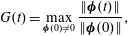 $$\begin{eqnarray}G(t)=\max _{\unicode[STIX]{x1D753}(0)\neq 0}\frac{\Vert \unicode[STIX]{x1D753}(t)\Vert }{\Vert \unicode[STIX]{x1D753}(0)\Vert },\end{eqnarray}$$
disregarding the pressure term in the energy norm calculation;
 $\Vert \;\Vert$
refers to the Euclidean norm. The time in the growth curves is normalised by
 $D/U_{x}$
, where
 $U_{x}$
is the peak of the mean velocity at the analysed axial station. The equation above is then solved using the eigenfunction expansion method described in Schmid & Henningson (Reference Schmid and Henningson2012), considering nearly all eigenfunctions; only those with spurious eigenvalues were discarded. The structure of the response at the time of optimal growth can be identified by this computation, as well as the initial disturbance that generates that field. Also, since the solution involves a singular value decomposition, the suboptimals at a given time can also be obtained in the same calculation. Note that no turbulent viscosity was added to the model for both resolvent and transient growth analyses.
4 Results
The results are divided into two distinct parts. In the first, we treat each cross-section of the jet separately, transforming the time variable
 $t$
into a pseudo-axial coordinate
 $x_{t}$
using Taylor’s hypothesis, as in Marusic, Baars & Hutchins (Reference Marusic, Baars and Hutchins2017). Moreover, the azimuthal coordinate
 $\unicode[STIX]{x1D703}$
is shown as a pseudo-span
 $z=r\unicode[STIX]{x1D703}$
. We obtain thus
 $(x_{t},z)$
fields, which are Fourier transformed and compared to results of boundary layer experiments so as to evaluate similarities between structures in a turbulent jet and the large-scale, elongated structures seen in turbulent boundary layers. In the second analysis, we use all the pairs
 $(x_{1},x_{2})$
of the experiments to build the cross-spectral matrix and obtain the SPOD modes for each azimuthal mode, leading to a further characterisation of the jet structures.
We then analyse the radial shapes of these structures. Slices of the SPOD modes are compared with the equivalent resolvent response modes at the same frequency and azimuthal wavenumber. The same results are then compared with transient growth responses at the time of optimal growth. In both analyses, the optimal forcing and optimal initial disturbances are analysed, relating the phenomena present in the turbulent jet with those found in wall-bounded turbulent flows.
4.1 Velocity fluctuations studied with Taylor’s hypothesis
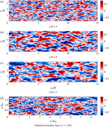
Three representative PIV planes (
 $x/D=3,5,7$
) are selected, and the time coordinate transformed using Taylor hypothesis,
 $x_{t}=tU_{ref}$
, where
 $U_{ref}$
is chosen to be the mean velocity at the radial station analysed (
 $r/D=0.55$
). A pseudo-spanwise coordinate
 $z$
is obtained by rescaling azimuth
 $\unicode[STIX]{x1D703}$
as
 $z=r\unicode[STIX]{x1D703}$
. Axial velocity fluctuations at the planes
 $(x_{t},z)$
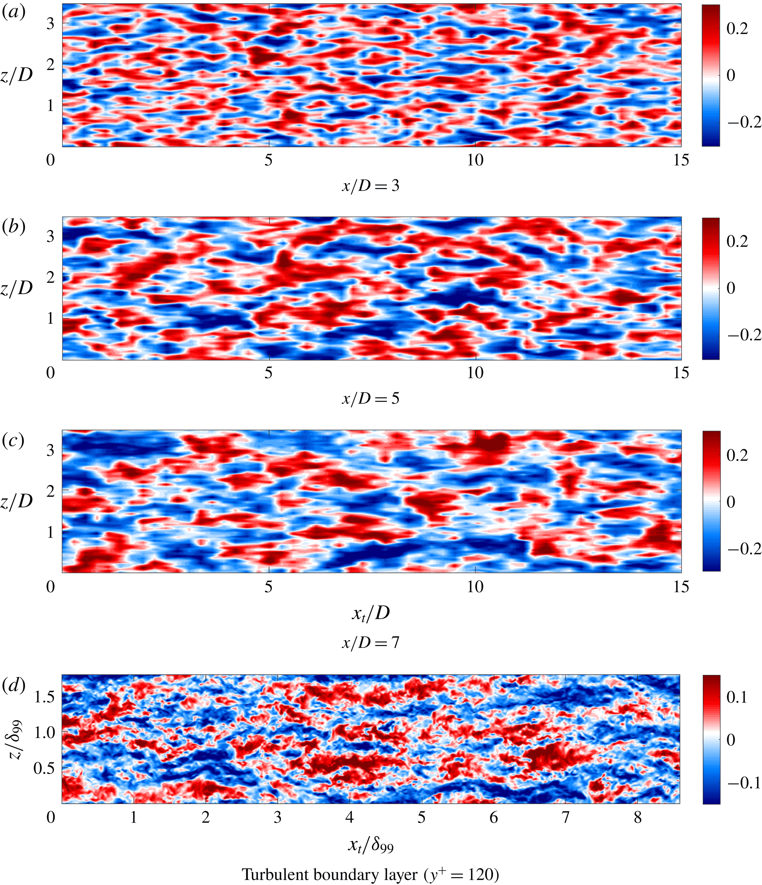
can be seen in figure 2.
Axial velocity fluctuations over a
 $(x_{t},z)$
plane for a
 $M=0.4$
jet for several axial stations (
 $x/D=3$
, 5, 7, respectively) and
 $r/D=0.55$
(a–c). The data were normalised by the mean streamwise velocity at the given radial station. Colour ranges from
 $-0.3$
to 0.3. Axial velocity fluctuations of large-eddy simulation results of a turbulent boundary layer at
 $y^{+}=120$
and
 $Re_{\unicode[STIX]{x1D6FF}_{\unicode[STIX]{x1D703}}}=4430$
(Eitel-Amor, Örlü & Schlatter Reference Eitel-Amor, Örlü and Schlatter2014) are also shown (d).
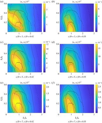
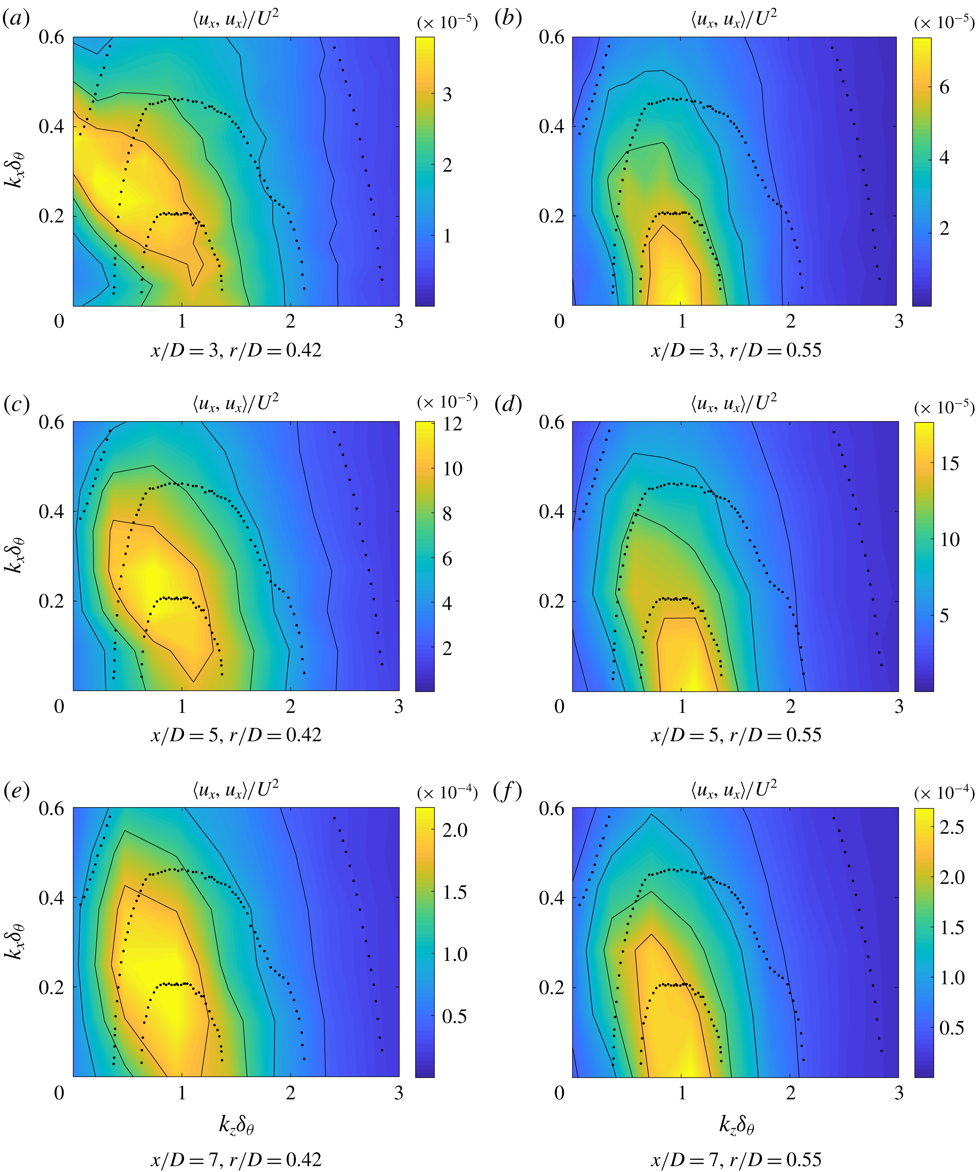
Energy spectrum (colours, full contours) in the
 $(k_{x},k_{z})$
domain for a
 $M=0.4$
jet for several axial stations (
 $x/D=3$
, 5, 7, respectively) and
 $r/D=0.42,0.55$
. A comparison with results from Tomkins & Adrian (Reference Tomkins and Adrian2005) is also shown (dotted contours). Spectrum axes are normalised by the momentum thickness
 $\unicode[STIX]{x1D6FF}_{\unicode[STIX]{x1D703}}$
.
Looking closely at figure 2, one can identify elongated streaky structures, resembling those found in wall-bounded flows, such as boundary layers (Hutchins & Marusic Reference Hutchins and Marusic2007), pipes (Hellström, Sinha & Smits Reference Hellström, Sinha and Smits2011) and channel flow (Monty et al.
Reference Monty, Stewart, Williams and Chong2007), usually associated with very large-scale motions or superstructures in wall-bounded turbulence studies (Smits et al.
Reference Smits, McKeon and Marusic2011). As is the case in turbulent boundary layers superstructures (Hutchins & Marusic Reference Hutchins and Marusic2007), the streaks meander in the axial direction in this free-shear flow. Also, the pseudo-spanwise wavelength changes from small values at positions near the nozzle, to larger values as the PIV measurement station is moved downstream; the streak width for
 $x/D=3$
is smaller than for the two other positions considered. This behaviour can be expected since, moving downstream, the shear-layer thickness also increases; the scaling of streak sizes with the local thickness is explored next. To highlight the resemblance of these streaks with the large-scale structures from turbulent boundary layers, we show the results from a large-eddy simulation performed by Eitel-Amor et al. (Reference Eitel-Amor, Örlü and Schlatter2014) at
 $y^{+}=120$
and
 $Re_{\unicode[STIX]{x1D6FF}_{\unicode[STIX]{x1D703}}}=4430$
in figure 2(d). Visually, these structures, that scale with the boundary layer thickness (
 $\unicode[STIX]{x1D6FF}_{99}$
), show high similarity to the ones shown here for turbulent jets.
From the fields depicted in figure 2, a spatial Fourier transform is performed in both the pseudo-axial and spanwise directions for
 $r/D=0.42$
and
 $r/D=0.55$
, using the mean velocity at each radial station as the reference velocity for Taylor’s hypothesis. The wavenumber spectra are shown in figure 3, from which some characteristics of the flow can be educed.
The first is that, for
 $r/D=0.42$
, the peak wavenumber is always located at
 $k_{x}\neq 0$
: it is already known that organised structures in the shape of axially extended wavepackets, with spatial evolution characterised by the Kelvin–Helmholtz instability, are present in this kind of flow (Cavalieri et al.
Reference Cavalieri, Rodríguez, Jordan, Colonius and Gervais2013; Jordan & Colonius Reference Jordan and Colonius2013). Nevertheless, considerable energy is also located at
 $k_{z}\neq 0$
, which constitutes the signature of the streaky structures described above. As the streamwise position of the PIV plane is moved downstream, the energy spectrum becomes progressively concentrated around a specific spanwise wavenumber (
 $k_{z}\unicode[STIX]{x1D6FF}_{\unicode[STIX]{x1D703}}\approx 1$
). The main cause of this change in the wavenumber peak is the growth and decay mechanism of wavepackets, the structures related to
 $k_{x}\neq 0$
and low
 $k_{z}$
: for regions near the nozzle, these structures have high amplitudes due to the high growth rate of the Kelvin–Helmholtz mode in regions of higher shear. These structures saturate and decay further downstream, causing their energy to decrease. On the other hand, the energy of the structures related to
 $k_{x}=0$
seems to grow as we move downstream. One important fact is that there is significant energy for
 $k_{x}\rightarrow 0$
and
 $k_{z}\unicode[STIX]{x1D6FF}_{\unicode[STIX]{x1D703}}\approx 1$
for all positions considered. Figure 3(b,d,f) shows the same spectrum for
 $r/D=0.55$
, a region where wavepackets have lower amplitudes; one can see that the peak wavenumber in the spanwise direction remains around
 $k_{z}\unicode[STIX]{x1D6FF}_{\unicode[STIX]{x1D703}}\approx 1$
, but now for
 $k_{x}=0$
. This is a sign that this region is not dominated by the wavepacket dynamics, but by the streamwise elongated structures seen in figure 2. Also, this result relates to what is visually perceived in figure 2: streaky structures have wavenumbers scaling with the local momentum thickness, and thus when plotted as a function of jet diameter one observes larger streaks at downstream stations.
To further highlight the relationship of these structures to those found in wall-bounded flows, we compare, in figure 3, the wavenumber spectrum of this flow with that of the turbulent boundary layer studied by Tomkins & Adrian (Reference Tomkins and Adrian2005). Even though the Reynolds number of the experiments differs (
 $Re_{\unicode[STIX]{x1D703}}=92542$
at
 $x/D=7$
for the present experiment and
 $Re_{\unicode[STIX]{x1D703}}=1015$
for the boundary layer), the peak position in the low
 $k_{x}$
region is very similar for both cases (around
 $k_{z}\unicode[STIX]{x1D6FF}_{\unicode[STIX]{x1D703}}=1$
), confirming that the structures found experimentally in the present case are similar to those that are ubiquitous to boundary layers, having even a comparable energy spectrum. Previous work (Bogey, Marsden & Bailly Reference Bogey, Marsden and Bailly2011; Cavalieri et al.
Reference Cavalieri, Rodríguez, Jordan, Colonius and Gervais2013) has highlighted this resemblance in the energy distribution via azimuthal Fourier-mode decomposition, showing similar peaks in the wavenumber spectrum with the proper scaling.
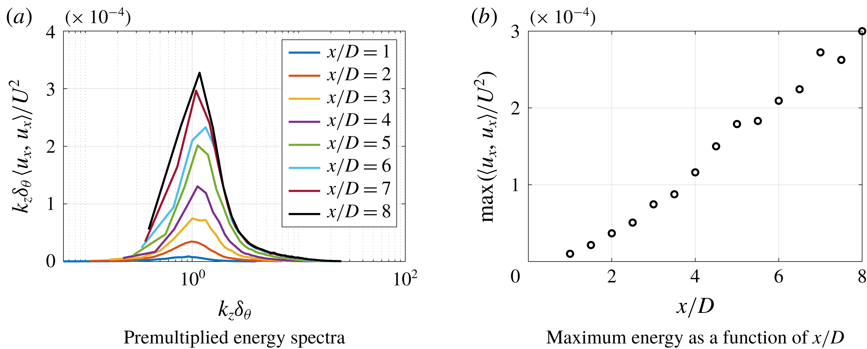
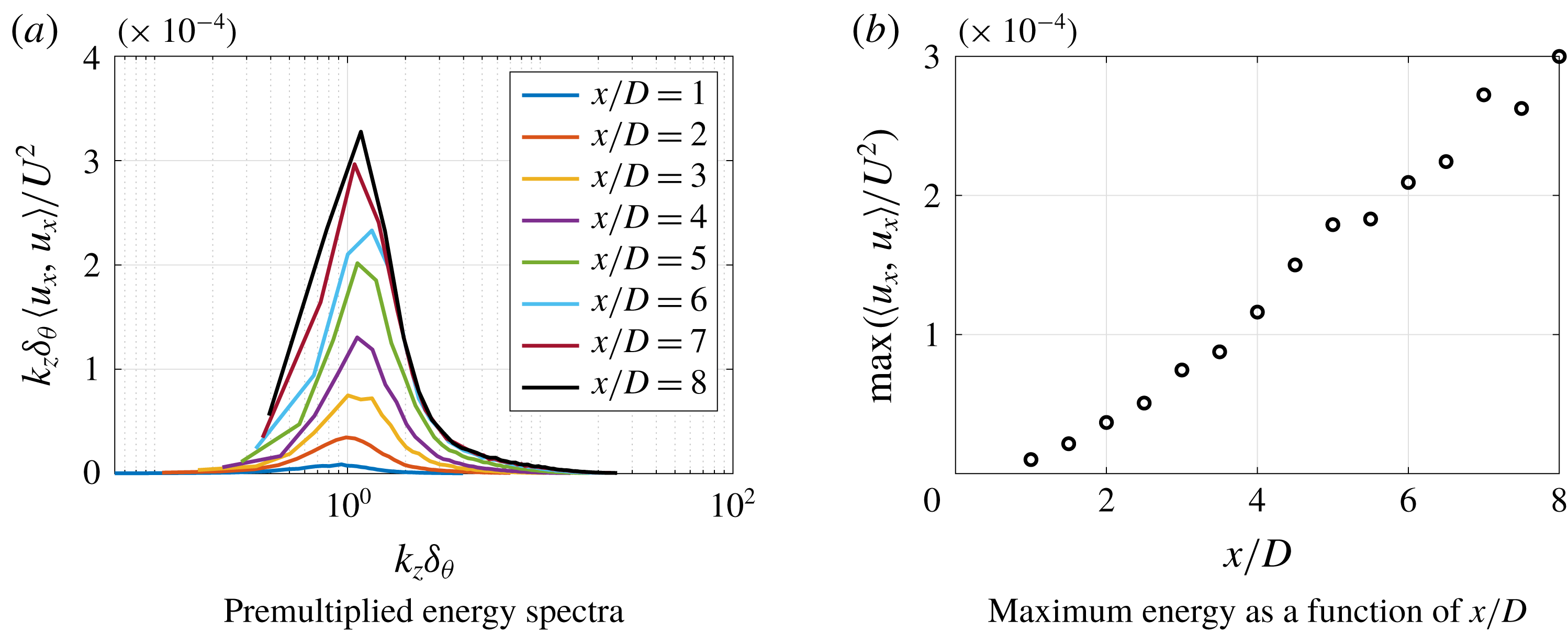
Finally, the premultiplied spectra for several axial positions of the PIV measurement,
 $k_{x}=0$
and
 $r/D=0.55$
can be seen in figure 4(a). The energy amplitudes of the streaks increase monotonically as we move the plane downstream, giving evidence that these structures are present with a higher amplitude in regions even further away from the nozzle, always peaking at the same value of
 $k_{z}\unicode[STIX]{x1D6FF}_{\unicode[STIX]{x1D703}}$
. The behaviour of the peak energy with the streamwise position of the PIV plane is shown in figure 4(b).
Spectra for
 $k_{x}=0$
and
 $r/D=0.55$
.
4.2 Spectral proper orthogonal decomposition
Solving the eigenvalue problem defined by (3.3) using standard methods, we can obtain the energy of each SPOD mode
 $\unicode[STIX]{x1D70E}_{n}(m,\unicode[STIX]{x1D714})$
and the respective eigenfunction
 $\unicode[STIX]{x1D709}^{(n)}(x,r,m,\unicode[STIX]{x1D714})$
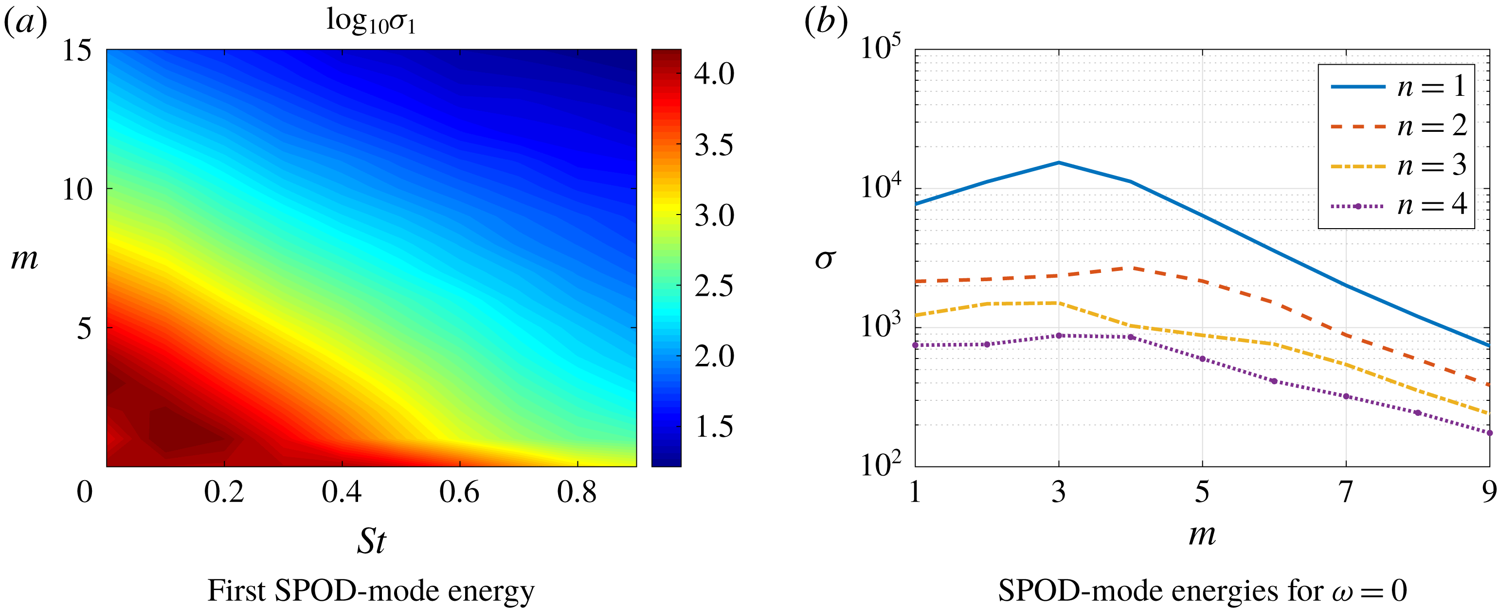
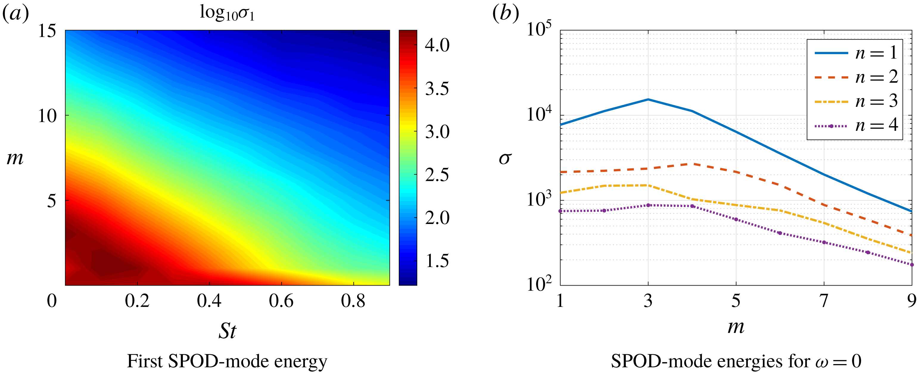
. Figure 5(a) shows the leading SPOD-mode energies for several Strouhal numbers
 $St=\unicode[STIX]{x1D714}D/(2\unicode[STIX]{x03C0}U_{jet})$
and azimuthal modes
 $m$
. The high-energy region for
 $m=0$
was shown to be related to a coherent wavepacket structure, as analysed by Semeraro et al. (Reference Semeraro, Jaunet, Jordan, Cavalieri and Lesshafft2016) and Lesshafft et al. (Reference Lesshafft, Semeraro, Jaunet, Cavalieri and Jordan2019), and is not the focus of the present work. Instead, we consider the
 $m>1$
region of the spectrum, where the reported streaky structures occur; in this region, the highest energies are found for
 $St=0$
(except for
 $m=1$
and 2), meaning that the structures are nearly steady in time, being related to a slow dynamic of the flow; here, SPOD modes for
 $St=0$
should be interpreted as the
 $St\rightarrow 0$
limit, with structures whose time scale is larger than the segment size used in Welch’s method. Even for
 $m=1$
and 2 the peak still occurs at low Strouhal numbers, supporting the hypothesis of a single mechanism. The energies of the first 4 SPOD modes for several azimuthal wavenumbers
 $m$
and
 $\unicode[STIX]{x1D714}=0$
can be seen in figure 5(b). As can be seen, a peak in
 $m=3$
arises for
 $n=1$
(which matches with the POD analysis performed by Hellström, Ganapathisubramani & Smits (Reference Hellström, Ganapathisubramani and Smits2015) for turbulent pipe flow) with a substantial separation between mode 1 and the suboptimals at the low
 $m$
region.
First SPOD energy for several Strouhal numbers and azimuthal modes (a) and SPOD energies for each azimuthal mode for
 $\unicode[STIX]{x1D714}=0$
(b).
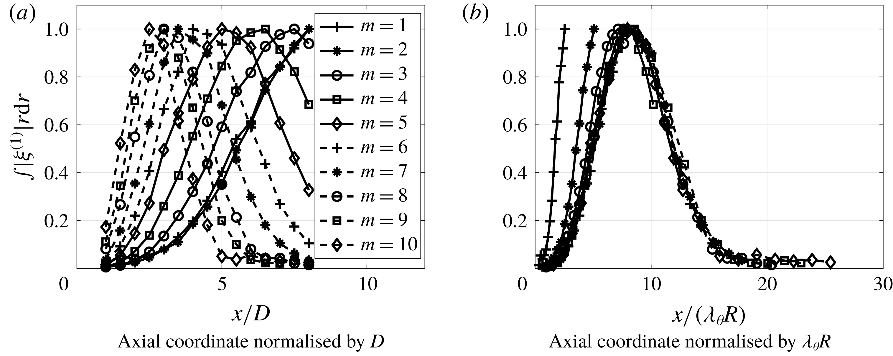
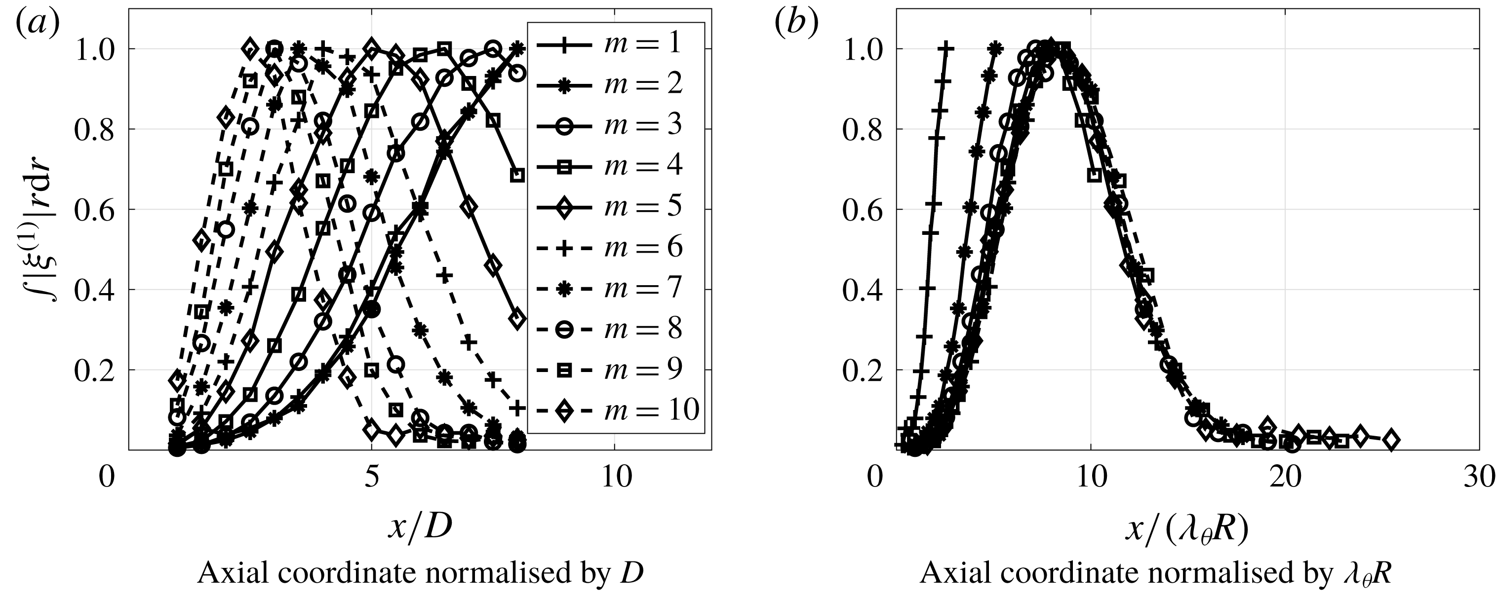
Following the analysis performed by Hellström, Marusic & Smits (Reference Hellström, Marusic and Smits2016), we define the azimuthal wavelength as
 $\unicode[STIX]{x1D706}_{\unicode[STIX]{x1D703}}=2\unicode[STIX]{x03C0}/m$
, which leads to a characteristic length of
 $\unicode[STIX]{x1D706}_{\unicode[STIX]{x1D703}}R$
, where
 $R=D/2$
. To obtain the characteristic streamwise development of the first SPOD mode, the eigenfunctions were radially integrated (
 $\unicode[STIX]{x1D6EF}(x)=\int |\unicode[STIX]{x1D709}^{(1)}|r\,\text{d}r$
) and then the axial coordinate was normalised using this new characteristic length. Normalising also the amplitude of each mode by its maximum, we find a collapse for these radially integrated first SPOD modes for azimuthal wavenumbers
 $m\geqslant 3$
. This underlines the fact that
 $\unicode[STIX]{x1D706}_{\unicode[STIX]{x1D703}}$
is the important length for the most energetic structures in this flow, highlighting the similarity with what is found for turbulent pipe flow in Hellström et al. (Reference Hellström, Marusic and Smits2016). However, the present analysis differs from the cited work mainly in the direction where this similarity was found; Hellström et al. (Reference Hellström, Marusic and Smits2016) found the disturbances in pipe flow to be self-similar in the radial direction, whereas we found a similarity and a characteristic length in the streamwise direction.
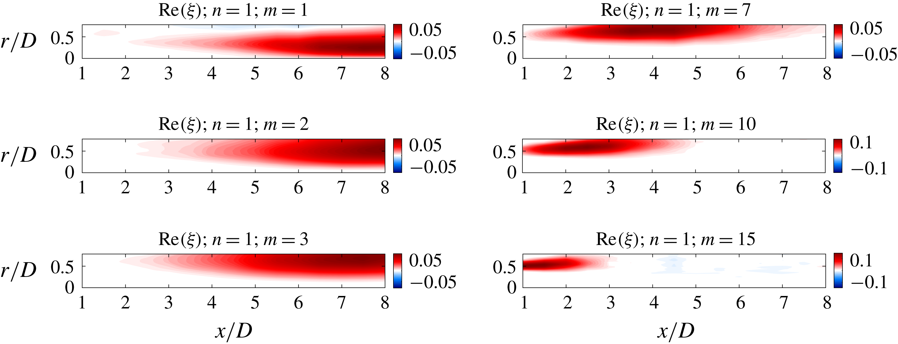
Shape of the first SPOD mode for several azimuthal modes.
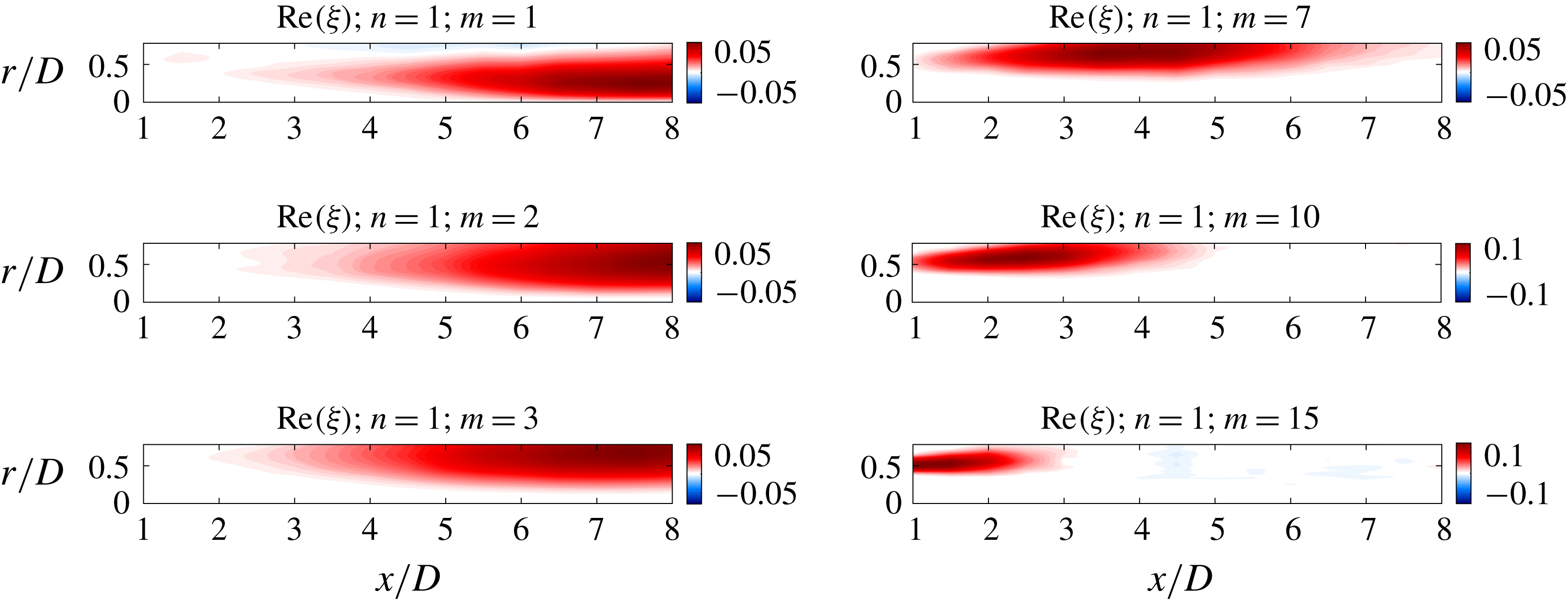
Streamwise velocity fluctuations of the first SPOD mode for several azimuthal modes.
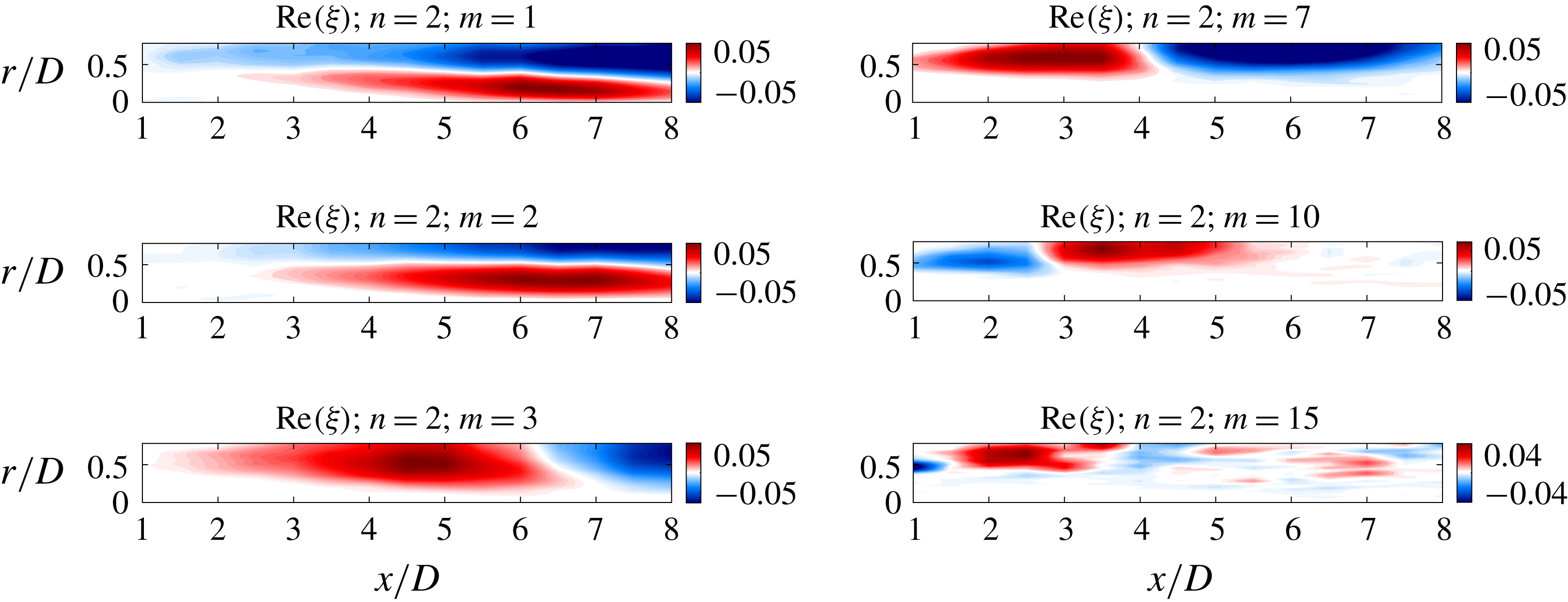
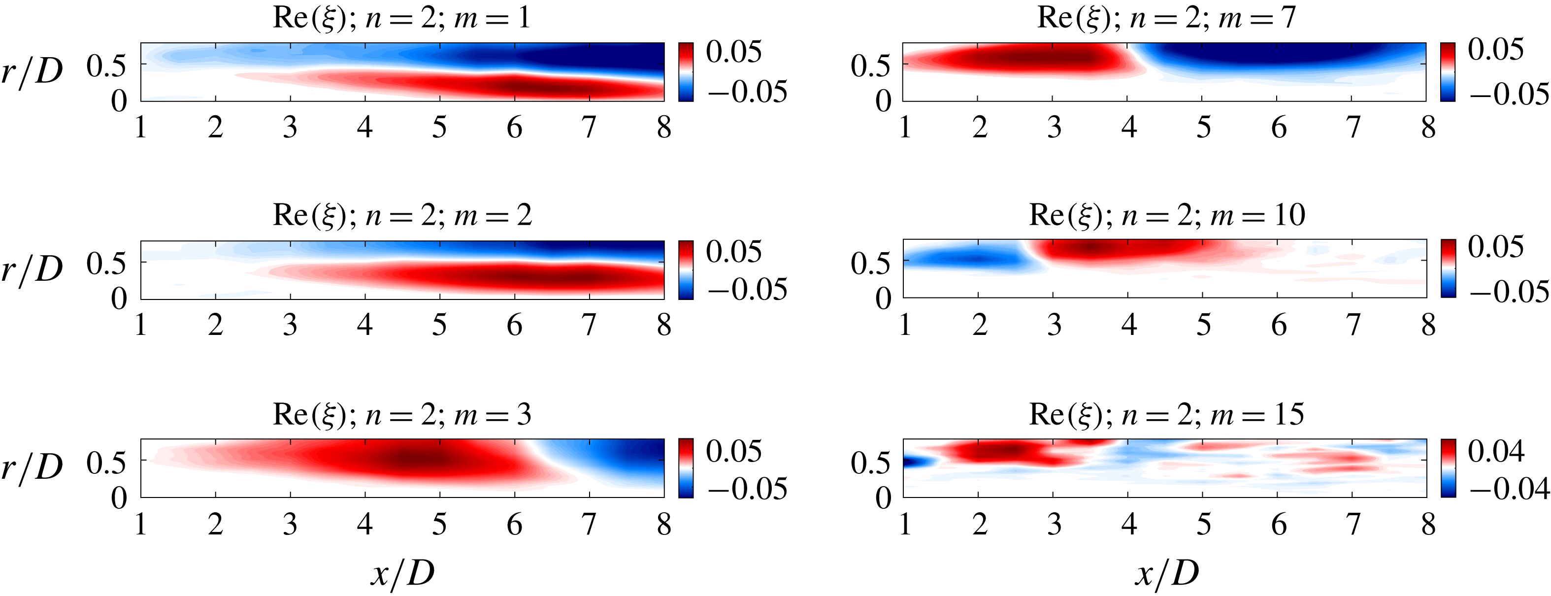
Streamwise velocity fluctuations of the second SPOD mode for several azimuthal modes.
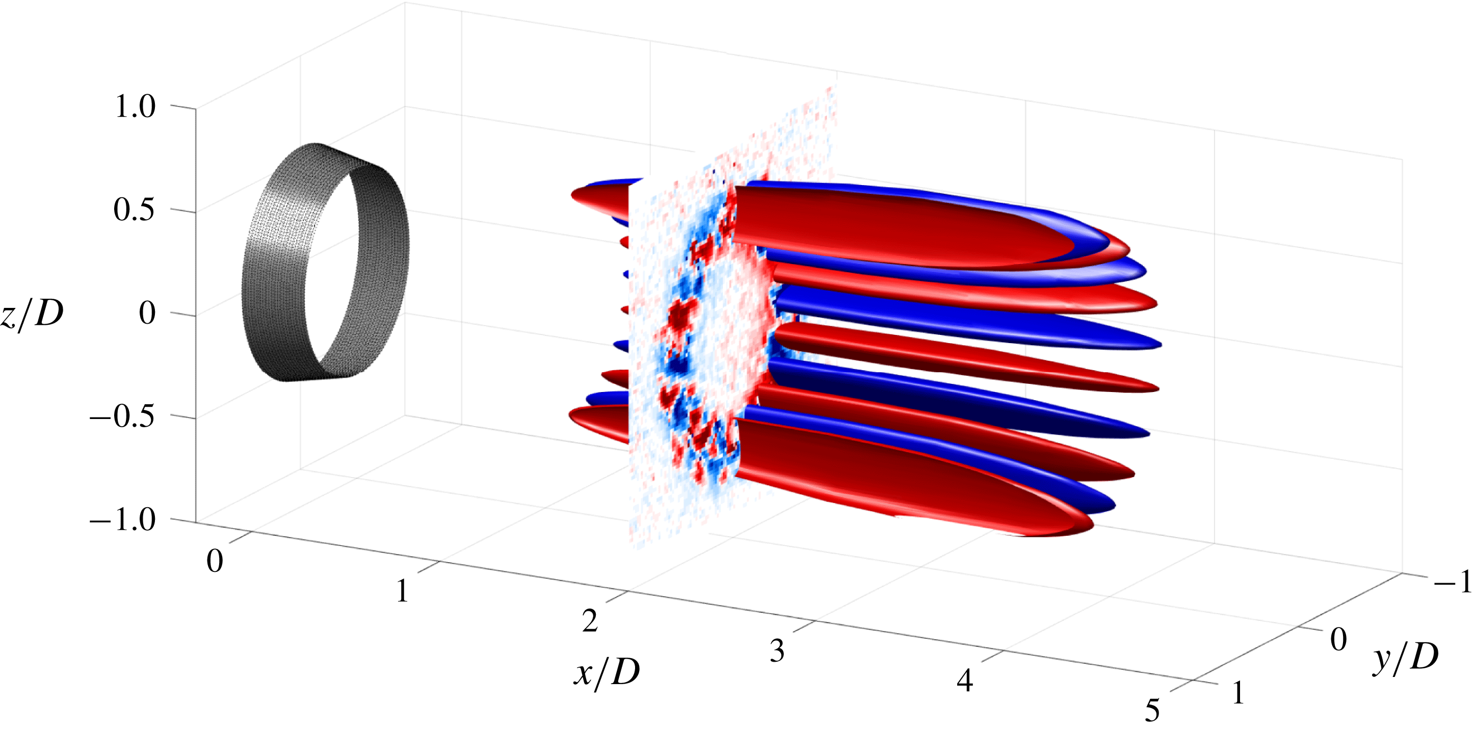
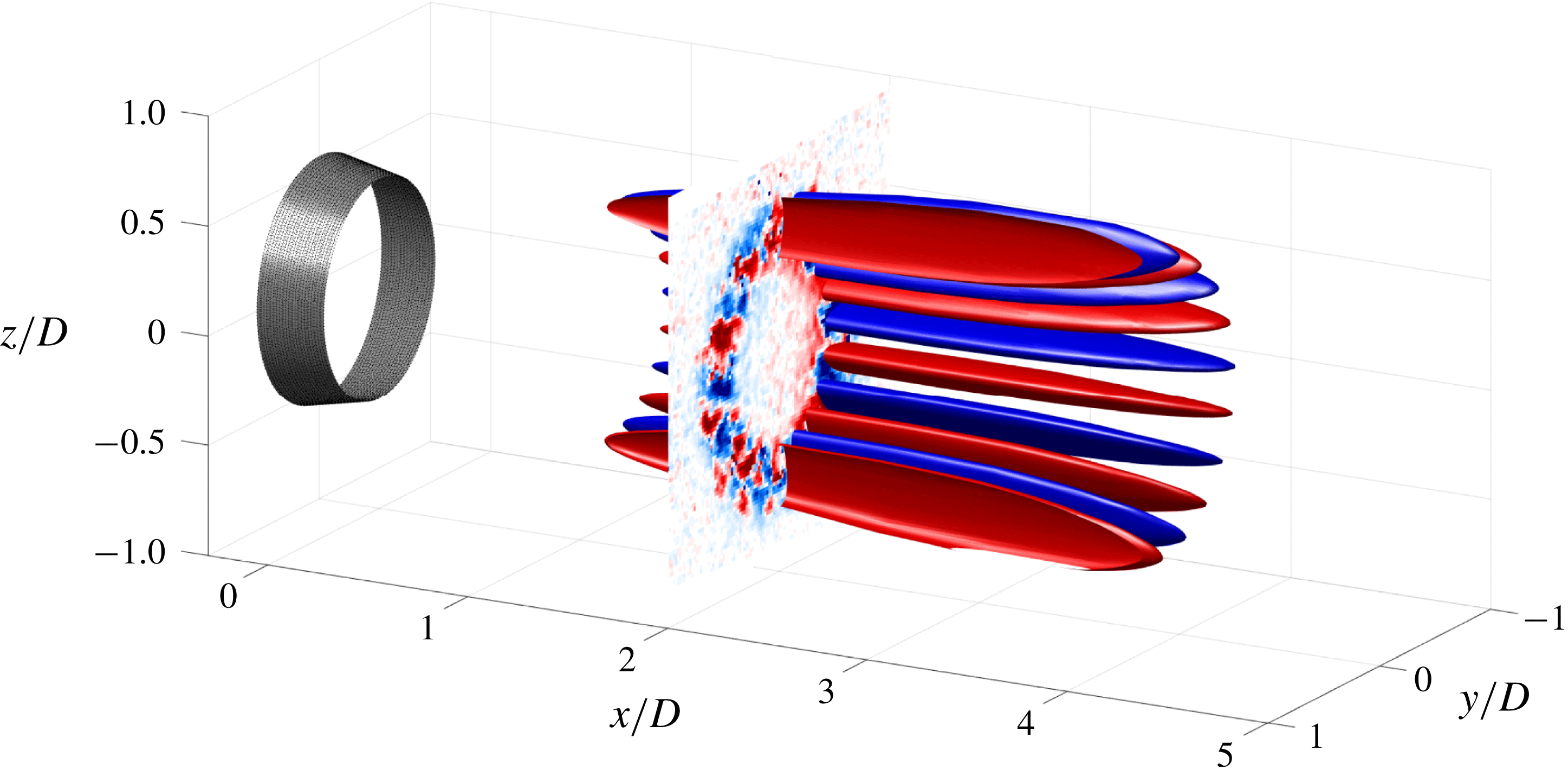
Isosurfaces of 40 % of the maximum amplitude of the first SPOD mode (positive values in red and negative ones in blue) and
 $m=10$
; contours rendered for
 $0<\unicode[STIX]{x1D719}<\unicode[STIX]{x03C0}$
for clarity. An instantaneous field from the experiments at
 $x/D=2$
is also depicted.
A striking feature of figure 6(a) is that the leading modes are very large-scale motions, extending several jet diameters in
 $x$
. For instance,
 $m=10$
structures have a length of approximately 5 jet diameters, and lower-
 $m$
modes are even larger than that. The aspect ratio of structures can be estimated through the collapse found in figure 6(b), and corresponds, for
 $m\geqslant 3$
, to a ratio of axial over azimuthal length equal to approximately 15, highlighting again the streaky shape of these modes.
The shapes of the first and second SPOD modes for
 $St=0$
and several azimuthal wavenumbers can be seen in figures 7 and 8. The main behaviour is similar for all modes: the structures start to grow from the near-nozzle region, at radial locations close to the shear layer, where linear mechanisms are expected to be relevant, and experience a substantial growth in space, with high amplitudes in different regions of the flow. As a consequence, we can identify the regions where each azimuthal mode is acting more effectively. For instance,
 $m=1$
and 2 are related to disturbances more concentrated at regions with
 $r/D<0.5$
and higher
 $x/D$
. The oscillations in the streamwise direction of the second SPOD mode for higher azimuthal wavenumbers, shown in figure 8, also support the idea that these modes are related to streaky structures, representing their meandering motion observed in figure 2 by the phase opposition between upstream and downstream positions. One can see that the first and second SPOD modes do not decay within the region covered by the measurements for
 $m=1$
; 2. Figure 7 also shows that all modes are located close to the nozzle as we increase the azimuthal wavenumber; this information, combined with the fact that streaks have higher amplitudes at downstream positions, which was inferred from figure 4(a), explains what is seen in the energy distribution of the SPOD modes: since lower azimuthal modes are related to more elongated structures, modes related to lower
 $m$
should be more energetic than the others at downstream positions.
On the other hand, for
 $m\geqslant 3$
, the modes have higher amplitudes close to the lipline, highlighting their action in the region of maximum shear. The axial support of the modes decreases with increasing
 $m$
, following the decrease of
 $\unicode[STIX]{x1D706}_{\unicode[STIX]{x1D703}}$
, as seen in figure 6, approaching progressively the nozzle. The fact that the peak position of these high azimuthal wavenumber streaks is in the upstream region indicates that these modes may well be captured by linear analysis. Particularly, the first SPOD mode for
 $m=10$
has a high amplitude at
 $x/D=2$
; figure 9 shows a sketch allowing this mode to be visualised with an instantaneous field at that position. It can be seen that the flow also possesses the oscillatory behaviour in azimuth, displaying an instantaneous cross-section of the streaky structures at that position with the correct radial support. Looking at lower radial positions, the signature of an
 $m=1$
streaky structure can also be identified, albeit with smaller amplitudes, which again agrees with the analysis of figure 7, since low-
 $m$
modes are more relevant for higher
 $x/D$
. The similarities between the structure of this mode and the instantaneous velocity field are clear, showing that these streaks are indeed present in snapshots of the turbulent jet.
In the present manuscript, we attempt to evaluate the correlation (or coherence) length of streaky structures using SPOD. It is also possible to use the cross-spectral density to evaluate length scales, similar to what is done by Jaunet et al. (Reference Jaunet, Jordan and Cavalieri2017); however, this requires taking specific choices for streamwise and radial positions, and a complete analysis for all possible positions becomes cumbersome. The use of SPOD circumvents these problems, as the dominant spatial structure in the whole cross-spectral density field is obtained in the leading eigenfunction. This allows a global estimate of length scales of dominant turbulent structures.
4.3 Comparison with linear models
We now focus on analysis of the radial shapes of the most energetic disturbances in the flow for
 $St=0$
and azimuthal wavenumbers
 $m=3$
,
 $m=7$
and
 $m=10$
at
 $x/D=2$
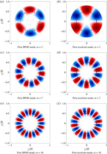
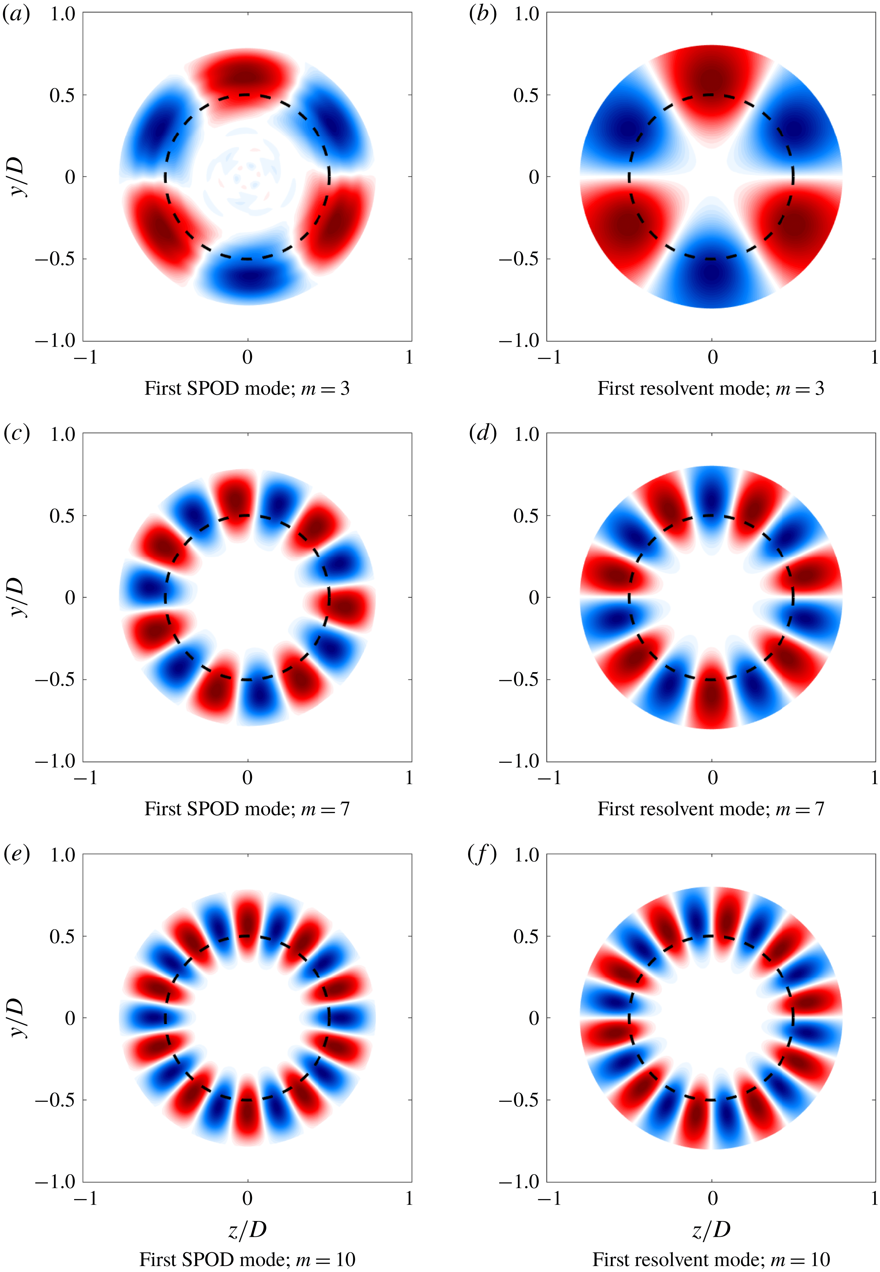
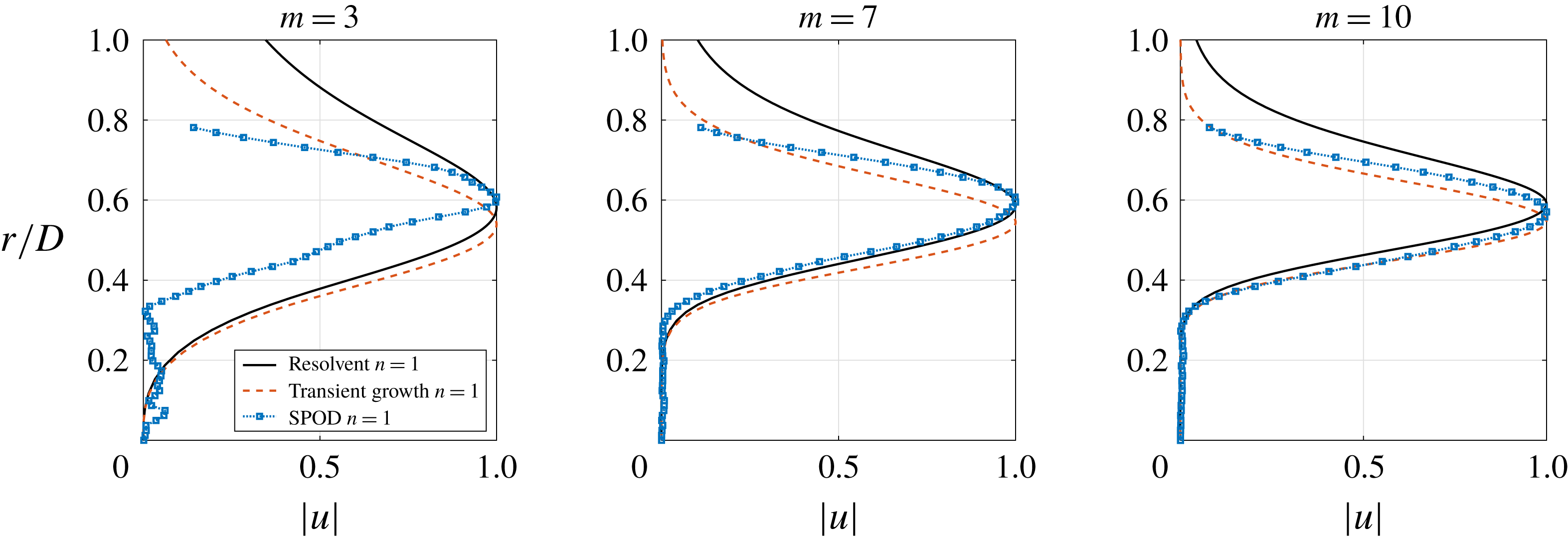
, a region where linear mechanisms are expected to be more relevant due to the higher shear. Cross-sections of the leading SPOD modes are shown in figure 10(a,c,e) and, for these azimuthal wavenumbers, it can be seen that most of mode dynamics is concentrated in the sheared region, especially around the lipline, with low amplitudes in the central region where the mean velocity is approximately uniform. As previously mentioned, the shapes of the SPOD modes are similar to what is found for turbulent pipe flow (Hellström et al.
Reference Hellström, Ganapathisubramani and Smits2015, Reference Hellström, Marusic and Smits2016); the main difference in the present flow is the absence of the wall, showing that this is not a sine qua non condition for the appearance of streaky structures in a flow and that the sheared mean flow of the jet alone supports their emergence, consistent with the analysis of Ellingsen & Palm (Reference Ellingsen and Palm1975). Another conclusion is that the radial decay of the structures is also fast. However, one should be careful in the analysis of the radial decay of the structures; since the PIV window covered the interval
 $0<r/D<0.8$
, structures with a radial support larger than that would be suppressed. Further analysis of the SPOD modes will be performed in the following sections, where a comparison between the most energetic structures with results from other tools (mostly used in wall-bounded turbulence analysis) will be performed. All analyses were performed using the experimental Reynolds number, considering the molecular viscosity.
First SPOD and resolvent modes for azimuthal wavenumbers
 $m=3$
,
 $m=7$
and
 $m=10$
(real part). Optimal responses from resolvent analysis are shown for the same radial interval of the experiments for comparison (
 $r/D<0.8$
). The dashed line indicates the position of the lipline.
4.3.1 Resolvent analysis
Using the formulation described in § 3.2, we obtain resolvent modes for the same frequency
 $\unicode[STIX]{x1D714}=0$
and wavenumbers
 $m=3;7;10$
for the
 $M=0.4$
jet at
 $x/D=2$
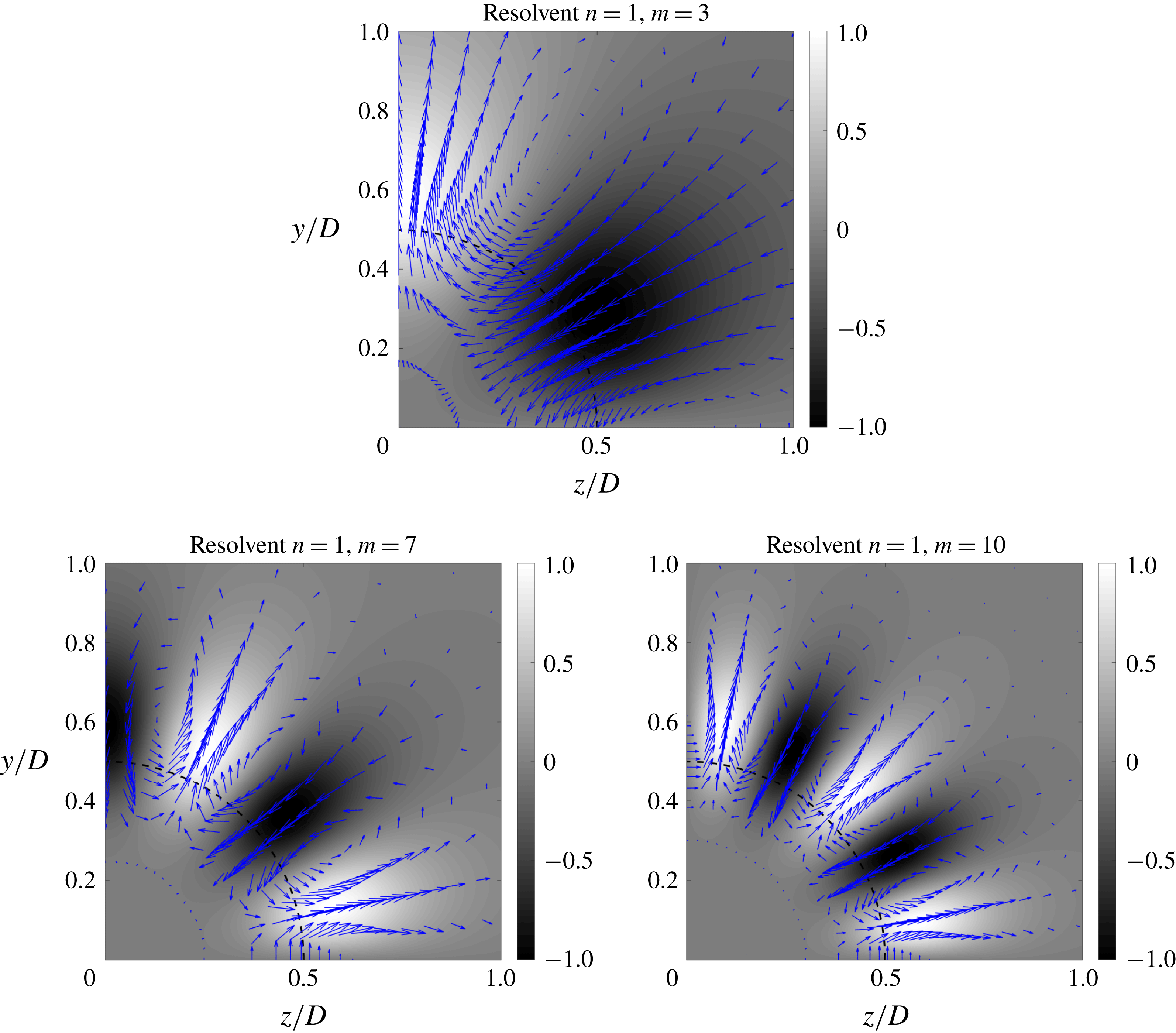
. The structures of the first mode can be seen in figure 10(b,d,f). We note that these plots retain the key characteristics of the SPOD modes, suggesting that these structures can be obtained via resolvent analysis of the turbulent mean. Comparing figures 10(b,d,f) and 10(a,c,e), we see a good agreement in terms of both the position of the peak for
 $m=7$
and 10, using the lipline as reference point, and the radial support of these modes. For
 $m=3$
, however, only the position of peak amplitude is captured by the resolvent analysis, which resulted in modes with radial shape that differ in width from the SPOD results. One of the reasons for that is the axial structure of the mode: as seen in figure 7, amplitudes of the leading
 $m=3$
SPOD mode at
 $x/D=2$
are rather low, and become more relevant only further downstream. The local resolvent analysis is expected to better match the SPOD results if these do not vary considerably in
 $x$
, since in the local resolvent analysis it is assumed that
 $k_{x}=0$
, which leads to constant amplitudes in
 $x$
. Still, even with this assumption, the local resolvent analysis is, on the whole, able to predict the shapes of the leading SPOD modes, particularly for higher azimuthal wavenumbers.
Another conclusion can be drawn from this analysis. It was shown by Semeraro et al. (Reference Semeraro, Jaunet, Jordan, Cavalieri and Lesshafft2016) and Towne et al. (Reference Towne, Schmidt and Colonius2018) that resolvent and SPOD modes should be identical if the nonlinear terms in the Navier–Stokes system are white in space. With that in mind, the resemblance between SPOD and resolvent modes in the present work suggests that the nonlinear terms at that position (considered as forcing herein), may be related to uncorrelated structures, that behave in the manner of white noise, at least for high azimuthal wavenumbers.
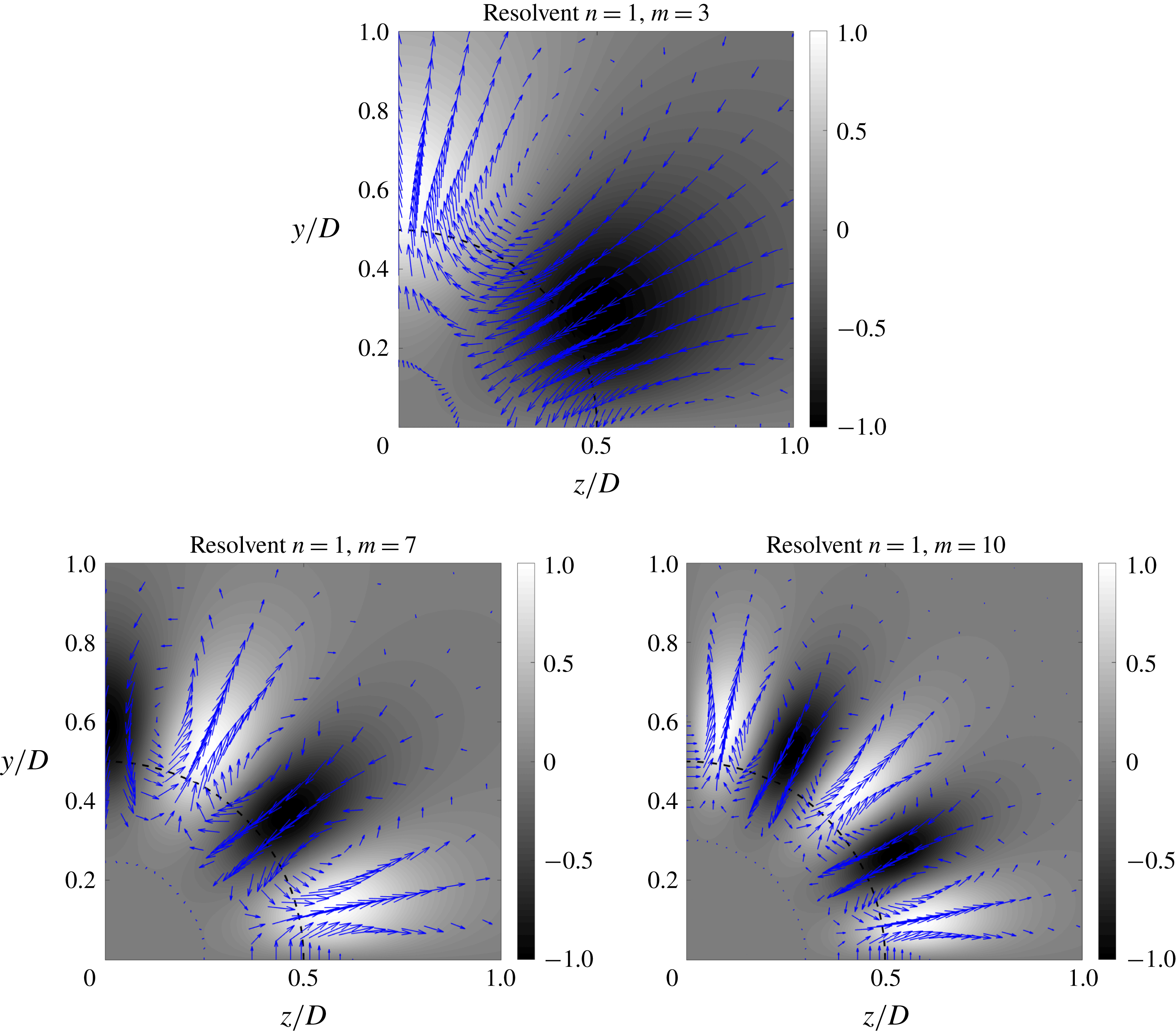
Information about the optimal forcing shape is also of interest. One should recall that, for wall-bounded flows, the growth of streaks via the lift-up effect plays an important role (Schmid & Henningson Reference Schmid and Henningson2012; Brandt Reference Brandt2014), and is one of the dominant phenomena in the flow dynamics. These streaks are forced by streamwise vortices (or rolls) in a particular manner: positive streaks are related to forcing that advects flow from faster to slower regions, with the opposite happening for negative streaks. This roll–streak dynamics is also suggested to be one of the building blocks that allows turbulence to self-sustain, as shown in Hamilton et al. (Reference Hamilton, Kim and Waleffe1995), Waleffe (Reference Waleffe1995) and Hwang & Bengana (Reference Hwang and Bengana2016). The optimal forcing from the resolvent analysis, and that leads to the streaky responses in figure 10(b,d,f), is shown in figure 11. The optimal forcing is seen to consist mainly of radial and azimuthal fluctuations; the streamwise component is negligible for the azimuthal wavenumbers studied here. We can see that the same lift-up mechanism occurs for the present case: whenever a positive streak occurs in the response mode, it is always related to the movement of fluid from fast to slow regions (or from the inner part of the jet to the outer region). The presence of these vortices in the forcing modes supports the hypothesis that the lift-up mechanism is also relevant for turbulent jets.
Radial and azimuthal components of the optimal forcing (arrows) and normalised streamwise component of optimal response (grey scale) from resolvent analysis for
 $m=3$
,
 $m=7$
and
 $m=10$
.
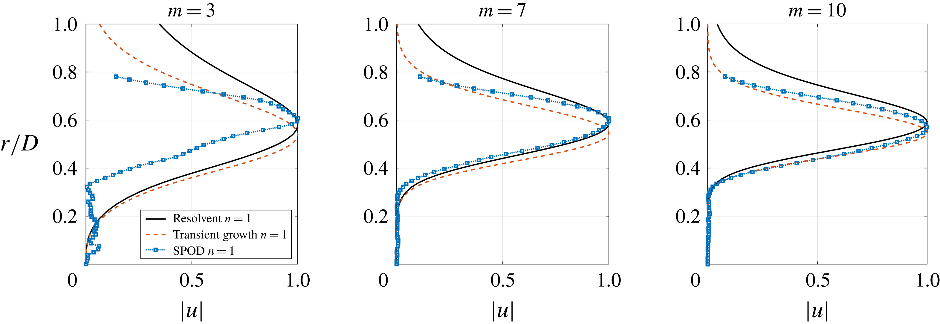
Comparison between SPOD modes (
 $\unicode[STIX]{x1D714}=0$
), response modes from resolvent analysis (
 $\unicode[STIX]{x1D714}=0$
,
 $k_{x}=0$
) and response at the time of optimal growth from transient growth analysis (
 $k_{x}=0$
). The optimal is shown for
 $m=3$
,
 $m=7$
and
 $m=10$
.
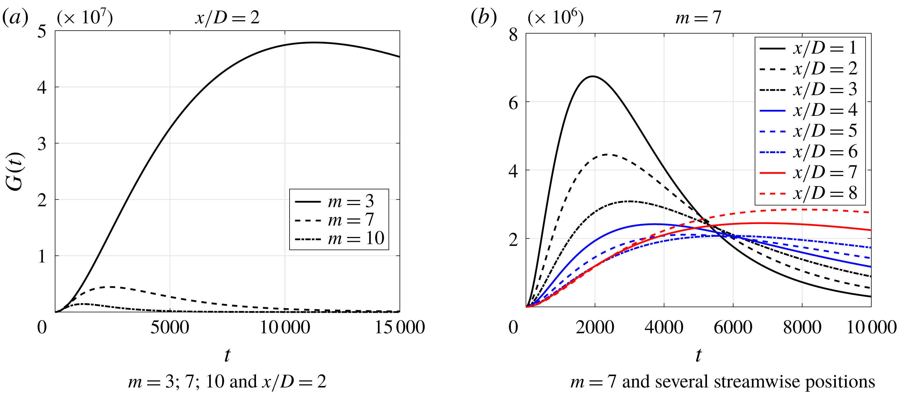
Growth curves from transient growth analysis (
 $k_{x}=0$
).
4.3.2 Transient growth
A transient growth study of Michalke’s velocity profiles for jets and slowly diffusing jet flows was performed by Jiménez-González & Brancher (Reference Jiménez-González and Brancher2017). In the present work, we extend the analysis to the turbulent jet, considering as base flow the experimental mean flow at
 $x/D=2$
, using an implementation similar to the resolvent analysis described in the previous section. We are thus not looking for initial disturbances in a laminar flow that will generate the largest growth, triggering transition, as in the cited work; we focus, rather, on turbulent structures with the largest transient growth in time, and which would then naturally emerge as large-scale structures. This amounts to an identification of the responses that predominate in the flow and the initial disturbances that lead to them. Also, using transient growth analysis, we obtain an idea of the time development of these disturbances, giving relevant information about the time scales over which this dynamics takes place.
The response at time of optimal growth for the transient growth analysis is similar to what was obtained by the resolvent analysis, with streaky structures concentrated close to the lipline. Figure 12 shows a comparison between the modes with optimal transient growth, those obtained by resolvent analysis and a cross-section of the global SPOD at
 $x/D=2$
. These plots emphasise the conclusions drawn in the previous section: the transient growth analysis captures well the peak position of the streaks for the cases studied and even the radial support of the modes is well represented for higher azimuthal modes (
 $m=7;10$
). It can also be seen that the structure of
 $m=3$
SPOD mode at this position has a much more experimental noise than in the other ones, which is probably due to its low relative amplitude at
 $x/D=2$
. Still, the optimal responses from both resolvent and transient growth analyses match the SPOD modes for the azimuthal wavenumbers studied, with improving results as
 $m$
increases.
One should recall that resolvent and SPOD modes were calculated for
 $\unicode[STIX]{x1D714}=0$
, focusing on structures that have a very slow evolution (not to say invariant) in time. On the other hand, transient growth involves a different approach: the nonlinear terms are set aside (there is no forcing) and we investigate initial disturbances that would have the highest growth for a given wavenumber. The fact that the present analysis shows a good agreement with resolvent modes is an indication that the dominant dynamics in this flow occurs in a low-frequency, low wavenumber range, and is thus a long-time behaviour. This suggests the possibility of using non-modal stability methods for turbulent jets not only for the low-energy wavepackets, but also for the high-energy structures, similar to the approaches used for wall-bounded flows.
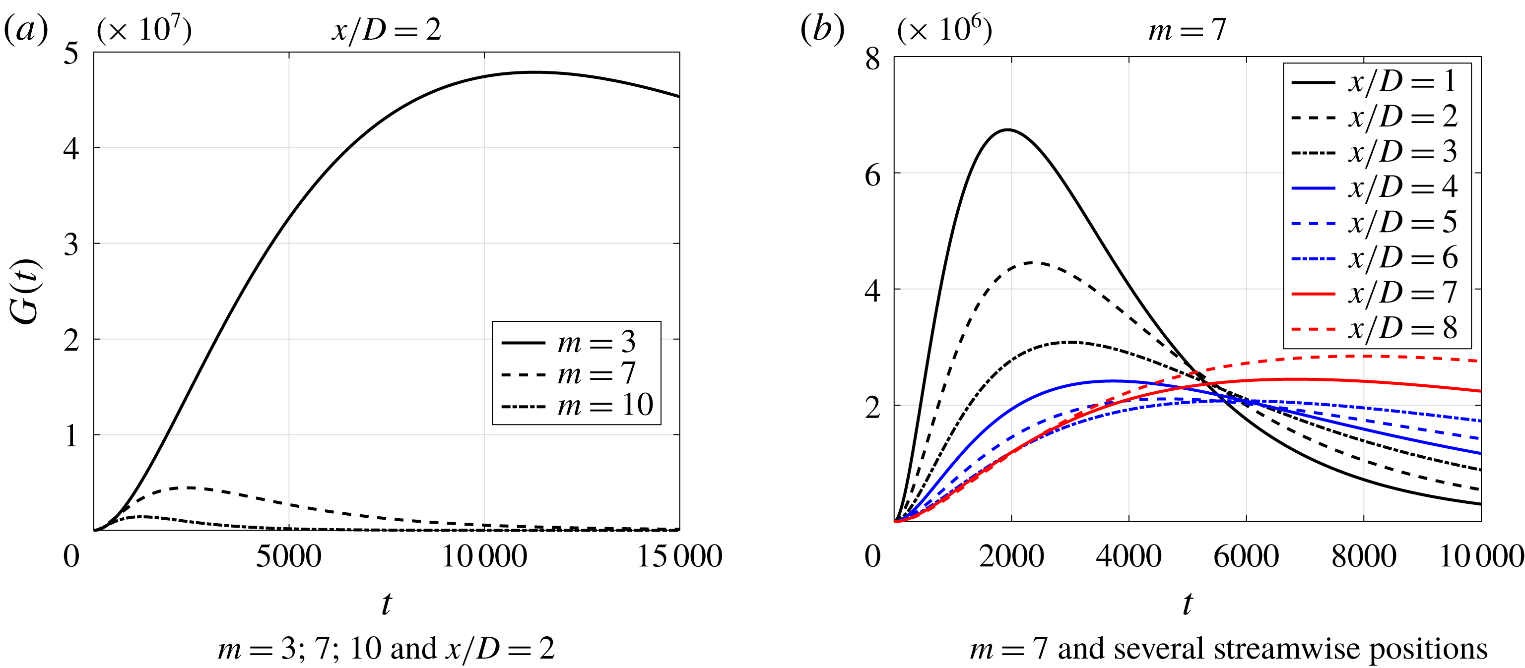
The slow dynamics of the phenomenon is supported by the growth curves for each case, depicted in figure 13(a). The large values of time for peak transient growth are also in accordance with the behaviour found by Jiménez-González & Brancher (Reference Jiménez-González and Brancher2017), who showed that the time of maximum growth scales with the Reynolds number; their results highlight a monotonic reduction of the optimal time of growth with increasing
 $m$
, which also agrees with the trend identified in figure 13(a). One should nonetheless bear in mind that, since this analysis is restricted to a slice of the jet, this time scale is not related to a streamwise vortex generated close to the nozzle, which would evolve in time and space and become the resulting streak. In the locally parallel framework, the time is related to a vortex initially generated at the same position as the resulting streak, clouding the link between this result and the real time evolution of the structure.
Figure 13(b) shows how the growth curve changes with the axial station of the base flow chosen for the calculation for
 $m=7$
, an azimuthal wavenumber whose first SPOD mode extends through the entire domain. This result shows that this linear mechanism is more relevant in regions closer to the nozzle, supporting our previous hypothesis. This behaviour is also similar to what was found by Jiménez-González & Brancher (Reference Jiménez-González and Brancher2017), who found smoother growth curves with lower optimal gains and higher optimal times for increasing shear layer momentum thickness; in our case, the momentum thickness of each axial section increases as we move downstream, leading to growth curves that have the same behaviour.
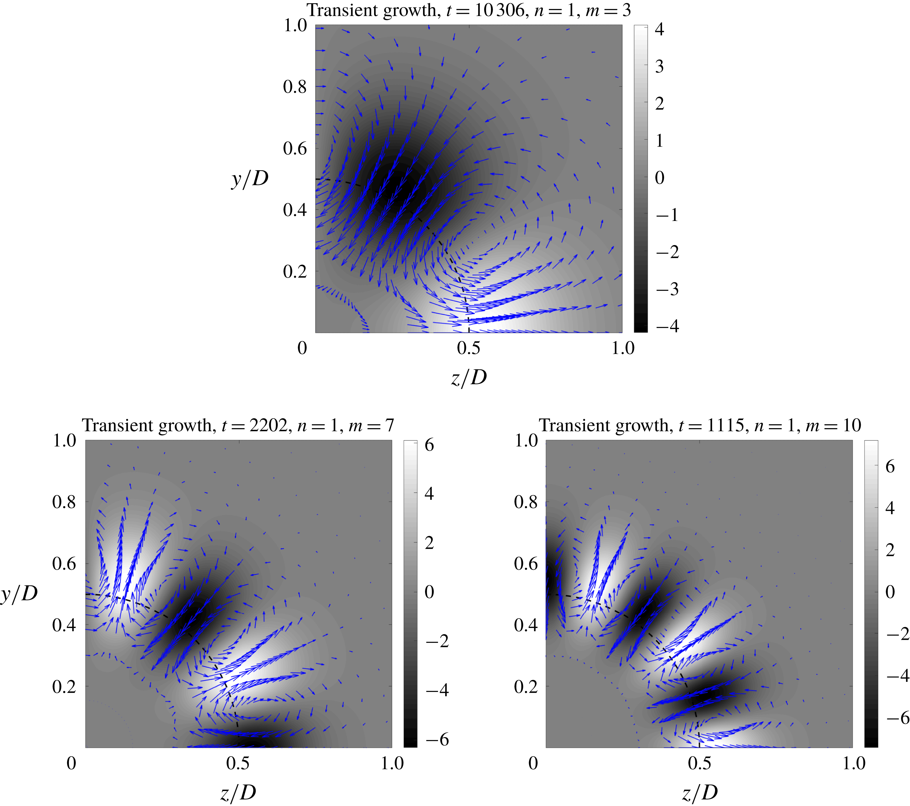
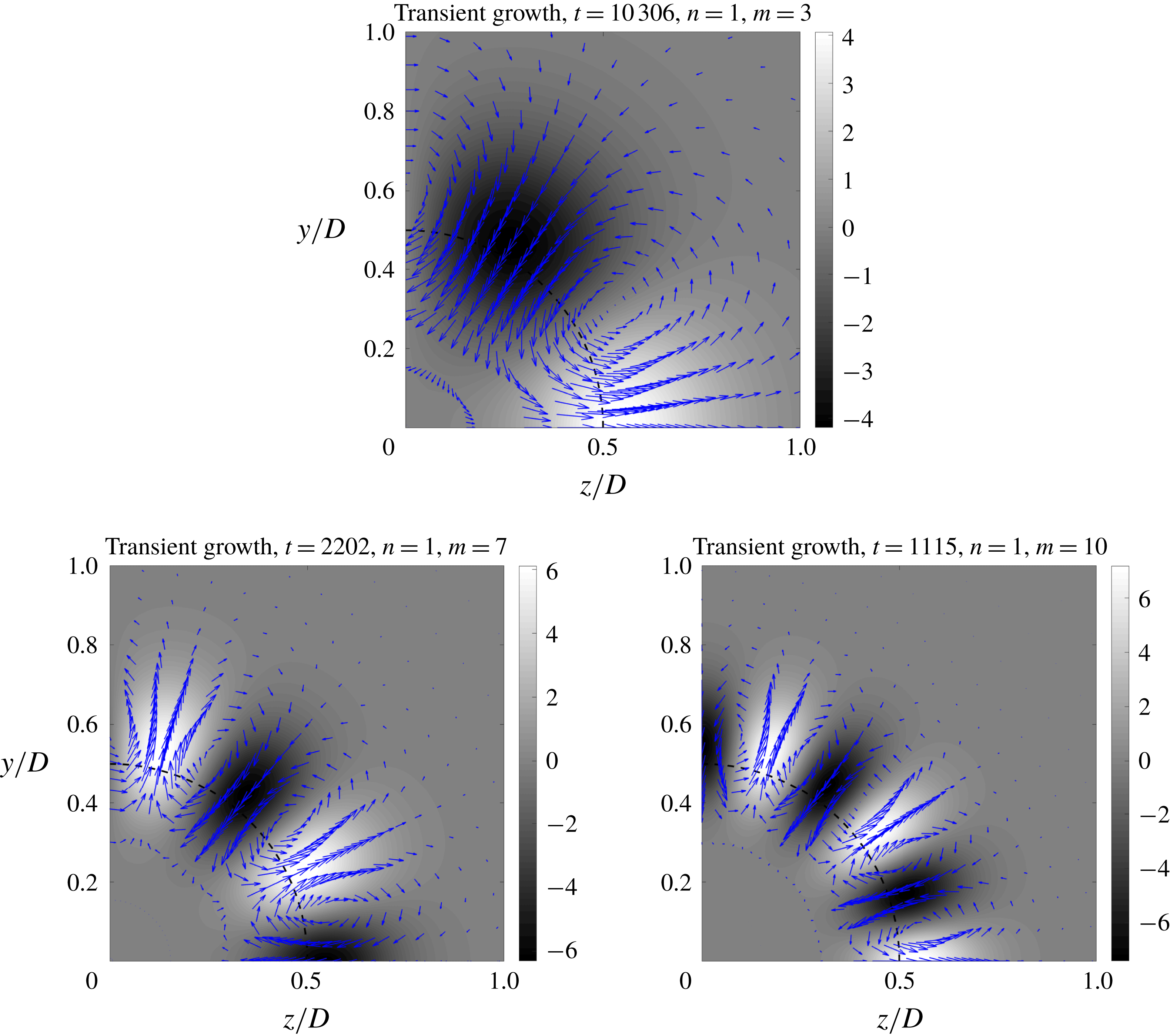
The initial disturbance that generates the optimally growing streaks can be seen in figure 14. The similarities with results from Jiménez-González & Brancher (Reference Jiménez-González and Brancher2017) and with the optimal forcing from the resolvent analysis confirms that the streaks are generated via the lift-up mechanism. Initial perturbations in the shape of streamwise vortices are those that will suffer the largest growth, evolving into streamwise elongated streaks, resembling those found by Cossu et al. (Reference Cossu, Pujals and Depardon2009). These vortices are also related to those found by Tinney et al. (Reference Tinney, Glauser and Ukeiley2008); the main novelty in the present study is their connection with the dominant streaks. Once again, the presence of these structures concentrated in the shear region, close to the lipline, is a suggestion that this, the lift-up mechanism, is related to any shear flow, not necessarily with the presence of a wall.
Radial and azimuthal components of the optimal initial disturbance (arrows) and streamwise component of optimal response (grey scale) from transient growth analysis for
 $m=3$
,
 $m=7$
and
 $m=10$
.
4.3.3 Streaks downstream of the potential core
In the previous sections we have chosen to perform the numerical analysis in regions closer to the nozzle, since the linear mechanisms we consider are expected to be stronger in this region due to the higher mean shear. Still, as shown in figures 6 and 7, these structures reach positions downstream of the potential core (
 $x/D>5.5$
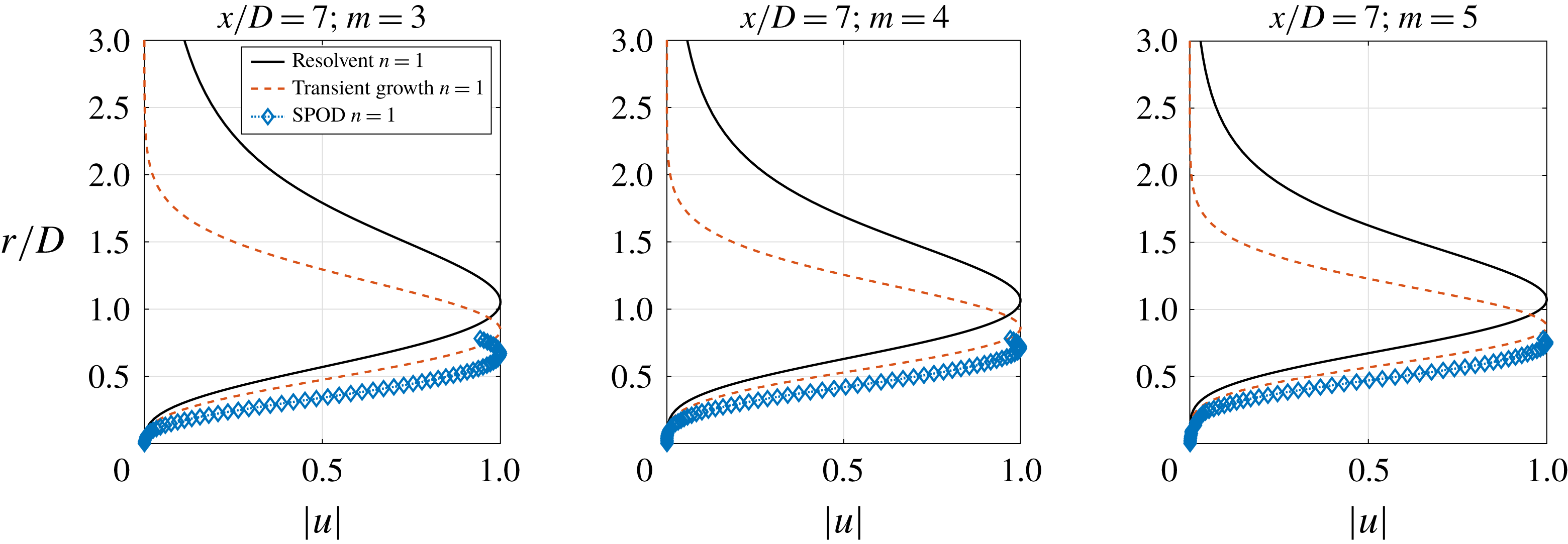
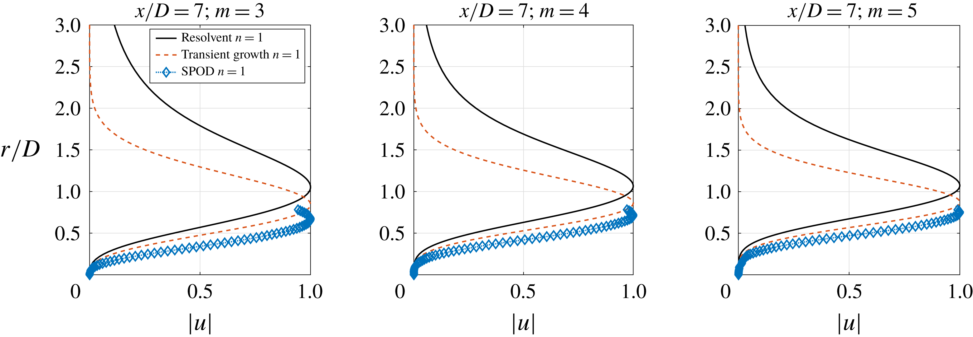
for this jet), especially for low azimuthal wavenumbers; we here evaluate if linear models are able to predict streak shapes in downstream locations. Figure 15 shows the comparison between the radial dependency of the SPOD modes at
 $x/D=7$
for
 $m=3$
; 4; 5 (wavenumbers for which the streaks have relevant amplitudes in this position) and the linear models using the base flow at this axial station, keeping the experimental Reynolds number in the analysis. At this position, the SPOD results show that the radial support of the most energetic structure considerably exceeds the measurement window, not only showing that streaks are larger in this region, but also making the analysis problematic, since about half of the radial information is lost. However, the models were able to qualitatively reproduce the sharp radial growth of the streak amplitude from the jet axis, with better results for transient growth analysis, especially for higher azimuthal wavenumbers.
Comparison between SPOD modes (
 $\unicode[STIX]{x1D714}=0$
), response modes from resolvent analysis (
 $\unicode[STIX]{x1D714}=0$
,
 $k_{x}=0$
) and response at the time of optimal growth from transient growth analysis (
 $k_{x}=0$
) for
 $x/D=7$
. The optimal is shown for
 $m=3$
,
 $m=4$
and
 $m=5$
.
5 Conclusions
In this work we have revisited the dual-plane, time-resolved, stereoscopic PIV database of a turbulent jet provided by Jaunet et al. (Reference Jaunet, Jordan and Cavalieri2017). We identify the presence of streamwise elongated, streaky structures in the turbulent field of a Mach 0.4 jet. To the best of our knowledge, this is the first time that turbulent streaks have been observed in turbulent jets. We have characterised the structures and highlighted similarities with those found in wall-bounded flows. The velocity fields (shown using Taylor hypothesis, as commonly done with experimental data of wall-bounded turbulence) exhibit a high resemblance with pipe flows and boundary layers, with the dominance of streaky structures, suggesting that the underlying mechanisms associated with such structures may be similar between jets and wall-bounded turbulence. Quantitative comparison of the energy spectrum with boundary layer experiments were also performed, showing again a similarity for the peak position of the spectrum. The growth of streaks in the axial direction was also inferred by the growth of the energy for
 $k_{x}=0$
as the PIV plane was moved downstream.
A spectral proper orthogonal decomposition of the streamwise velocity fluctuations clarified which modes are most relevant in the physical space of the experiment and how each mode was extended in the streamwise direction. Moreover, a scaling law, similar to that found by Hellström et al. (Reference Hellström, Marusic and Smits2016), was obtained, leading to a collapse of mode shapes for azimuthal wavenumbers
 $m\geqslant 3$
, showing that these structures are also self-similar in the streamwise direction.
Cross-sections of the leading SPOD mode were compared with optimal flow responses from resolvent and transient growth analyses. Resolvent modes and SPOD modes are in agreement for the peak position and radial shape, with some discrepancies for radial positions
 $r/D>0.6$
. The reasonable agreement obtained between the experimental SPOD and the resolvent indicates that the real forcing is likely to be a white noise in space, but improvement could be obtained if more realistic statistics of the nonlinear terms were used. The shape of the optimal forcing and corresponding response relates the observed structures with the widely studied lift-up effect: for the turbulent jet, the forcing takes the form of streamwise vortices with velocities directed such that flow is moved from high- to low-speed regions, generating a positive streak; the opposite occurs for the appearance of a negative streak.
Even though transient growth analysis involves different assumptions, considering initial disturbances that lead to maximum growth in time, a good agreement was found for the optimal response and the SPOD modes. Results indicate structures of low frequency and wavenumber, characterised by a slow evolution in time. The optimal initial disturbance has a shape close to the optimal forcing from resolvent analysis, allowing a clearer connection with the lift-up effect studied in several other works, especially for wall-bounded flows (see Brandt (Reference Brandt2014) and references therein).
Altogether, the results herein identify the presence of streaks in a high Reynolds number, turbulent jet, displaying a direct connection with the lift-up effect. They show that this phenomenon is also present in natural unbounded flows such as jets, showing that the only element necessary for lift-up to occur is the presence of shear in a flow, meaning that the existence of a wall is not a sine qua non condition for the occurrence of streaks in turbulent flows. Moreover, since these coherent structures exist at the same time as the well-known Kelvin–Helmholtz wavepacket, they may be related to some of the features already studied in that framework. As observed by Liepmann & Gharib (Reference Liepmann and Gharib1992), axisymmetric Kelvin–Helmholtz vortices in transitional jets have secondary instabilities leading to the appearance of streamwise vortices, which may provide the required forcing leading to streaky structures. On the other hand, for transitional flows it was also observed that streaks have a stabilising effect on Kelvin–Helmholtz vortices (Marant & Cossu Reference Marant and Cossu2018). From such studies, a promising direction for turbulent jets would be on a possible interplay between Kelvin–Helmholtz wavepackets, streamwise vortices and elongated streaks, since this could be responsible for wavepacket jitter and corresponding coherence decay (Cavalieri et al. Reference Cavalieri, Jordan, Agarwal and Gervais2011; Cavalieri & Agarwal Reference Cavalieri and Agarwal2014).
Another interesting direction is the connection of the present findings to the dynamics of non-circular jets. In particular, nozzles serrations, or chevrons, are known to lead to streamwise vortices, which in turn modify the jet mean flow (Gutmark & Grinstein Reference Gutmark and Grinstein1999; Alkislar, Krothapalli & Butler Reference Alkislar, Krothapalli and Butler2007). This could be thought as the generation of steady streaks, which persist downstream, and tend to stabilise Kelvin–Helmholtz wavepackets (Lajús, Cavalieri & Deschamps Reference Lajús, Cavalieri and Deschamps2015; Sinha et al. Reference Sinha, Gudmundsson, Xia and Colonius2016; Marant & Cossu Reference Marant and Cossu2018). Such steady streaky structures have been studied in turbulent boundary layers and related to the lift-up mechanism (Pujals, Cossu & Depardon Reference Pujals, Cossu and Depardon2010). The optimal forcings studied here could serve to guide nozzle design, increasing inhomogeneities of the shear layer in the azimuthal direction. Further work following this direction for turbulent jets is promising.
Acknowledgements
P.A.S.N was funded by a CNPq scholarship. A.C. acknowledges financial support by CNPq (grant no. 310523/2017-6). We ackowledge Professors D. S. Henningson and A. Hanifi for the helpful insights in the discussions. We also thank Professor P. Schlatter for providing results of large-eddy simulation of a turbulent boundary layer.
Appendix A
The underlying operators in § 3.2 were based on McKeon & Sharma’s (Reference McKeon and Sharma2010) formulation and are defined below. The matrix
 $\unicode[STIX]{x1D63C}$
, which accounts for the evolution of velocities, is given by
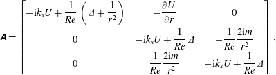 $$\begin{eqnarray}\unicode[STIX]{x1D63C}=\left[\begin{array}{@{}ccc@{}}-\text{i}k_{x}U+{\displaystyle \frac{1}{Re}}\left(\unicode[STIX]{x1D6E5}+{\displaystyle \frac{1}{r^{2}}}\right) & -{\displaystyle \frac{\unicode[STIX]{x2202}U}{\unicode[STIX]{x2202}r}} & 0\\ 0 & -\text{i}k_{x}U+{\displaystyle \frac{1}{Re}}\unicode[STIX]{x1D6E5} & -{\displaystyle \frac{1}{Re}}{\displaystyle \frac{2\text{i}m}{r^{2}}}\\ 0 & {\displaystyle \frac{1}{Re}}{\displaystyle \frac{2\text{i}m}{r^{2}}} & -\text{i}k_{x}U+{\displaystyle \frac{1}{Re}}\unicode[STIX]{x1D6E5}\end{array}\right],\end{eqnarray}$$
where
 $\unicode[STIX]{x1D6E5}=-k_{x}^{2}-((m^{2}+1)/r^{2})+(\unicode[STIX]{x2202}^{2}/\unicode[STIX]{x2202}r^{2})+(1/r)(\unicode[STIX]{x2202}/\unicode[STIX]{x2202}r)$
. In order to consider the pressure term in the formulation, the following operators are defined:
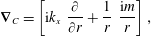 $$\begin{eqnarray}\displaystyle & \displaystyle \unicode[STIX]{x1D735}_{C}=\left[\text{i}k_{x}\;\;\frac{\unicode[STIX]{x2202}}{\unicode[STIX]{x2202}r}+\frac{1}{r}\;\;\frac{\text{i}m}{r}\right], & \displaystyle\end{eqnarray}$$
 $$\begin{eqnarray}\displaystyle & \displaystyle \unicode[STIX]{x1D735}=\left[\begin{array}{@{}c@{}}\text{i}k_{x}\\ {\displaystyle \frac{\unicode[STIX]{x2202}}{\unicode[STIX]{x2202}r}}\\ {\displaystyle \frac{\text{i}m}{r}}\end{array}\right], & \displaystyle\end{eqnarray}$$
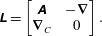
which are responsible for both the inclusion of the pressure and the continuity equation. Finally, the operator
 $\unicode[STIX]{x1D647}$
of the linearised Navier–Stokes equations is defined as
 $$\begin{eqnarray}\unicode[STIX]{x1D647}=\left[\begin{array}{@{}cc@{}}\unicode[STIX]{x1D63C} & -\unicode[STIX]{x1D735}\\ \unicode[STIX]{x1D735}_{C} & 0\end{array}\right].\end{eqnarray}$$
In order to isolate the time derivatives only in the velocity vector, we define the following matrix:
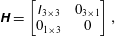 $$\begin{eqnarray}\unicode[STIX]{x1D643}=\left[\begin{array}{@{}cc@{}}\unicode[STIX]{x1D610}_{3\times 3} & 0_{3\times 1}\\ 0_{1\times 3} & 0\end{array}\right],\end{eqnarray}$$
where
 $\unicode[STIX]{x1D610}_{3\times 3}$
is a
 $3\times 3$
identity matrix and
 $0_{3\times 1}$
,
 $0_{1\times 3}$
are vectors of zeros (dimension
 $3\times 1$
and
 $1\times 3$
, respectively). Similarly, we define matrix
 $\unicode[STIX]{x1D63D}$
, which takes the forcing vector to a compact form
 $$\begin{eqnarray}\unicode[STIX]{x1D63D}=\left[\begin{array}{@{}c@{}}\unicode[STIX]{x1D610}_{3\times 3}\\ 0_{1\times 3}\end{array}\right].\end{eqnarray}$$
Finally, the filtering matrix that isolates only the streamwise velocity for the resolvent analysis is defined as:
 $$\begin{eqnarray}\unicode[STIX]{x1D63E}=\left[\begin{array}{@{}cc@{}}\unicode[STIX]{x1D610} & 0\\ 0 & 0_{3\times 3}\end{array}\right].\end{eqnarray}$$
The boundary conditions were implemented as in Lesshafft & Huerre (Reference Lesshafft and Huerre2007) and are dependent on the azimuthal mode as follows:
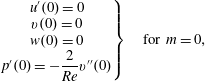 $$\begin{eqnarray}\displaystyle & \displaystyle \left.\begin{array}{@{}c@{}}u^{\prime }(0)=0\\ v(0)=0\\ w(0)=0\\ p^{\prime }(0)=-{\displaystyle \frac{2}{Re}}v^{\prime \prime }(0)\end{array}\right\}\quad \text{for }m=0, & \displaystyle\end{eqnarray}$$
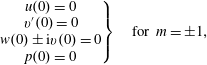 $$\begin{eqnarray}\displaystyle & \displaystyle \left.\begin{array}{@{}c@{}}u(0)=0\\ v^{\prime }(0)=0\\ w(0)\pm \text{i}v(0)=0\\ p(0)=0\end{array}\right\}\quad \text{for }m=\pm 1, & \displaystyle\end{eqnarray}$$
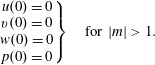 $$\begin{eqnarray}\displaystyle & \displaystyle \left.\begin{array}{@{}c@{}}u(0)=0\\ v(0)=0\\ w(0)=0\\ p(0)=0\end{array}\right\}\quad \text{for }|m|>1. & \displaystyle\end{eqnarray}$$