



1. Introduction
Vortex nucleation in superfluids and its resulting drag has been observed experimentally in strongly interacting He-II and weakly interacting Bose–Einstein condensates (Craig & Pellam Reference Craig and Pellam1957; Madison et al. Reference Madison, Chevy, Wohlleben and Dalibard2000; Raman et al. Reference Raman, Abo-Shaeer, Vogels, Xu and Ketterle2001; Anderson Reference Anderson2010; Neely et al. Reference Neely, Samson, Bradley, Davis and Anderson2010; Desbuquois et al. Reference Desbuquois, Chomaz, Yefsah, Leonard, Beugnon, Weitenberg and Dalibard2012; Kwon et al. Reference Kwon, Moon, Seo and Shin2015, Reference Kwon, Kim, Seo and Shin2016; Park, Ko & Shin Reference Park, Ko and Shin2018; Gauthier et al. Reference Gauthier, Reeves, Yu, Bradley, Baker, Bell, Rubinsztein-Dunlop, Davis and Neely2019; Johnstone et al. Reference Johnstone, Groszek, Starkey, Billington, Simula and Helmerson2019). The Gross–Pitaevskii equation (GPE) (Gross Reference Gross1961; Pitaevskii Reference Pitaevskii1961) is a nonlinear Schrödinger equation that describes the latter situation, which can be mapped onto equivalent hydrodynamical equations using the transformation proposed by Madelung (Reference Madelung1927). This yields a potential/irrotational flow, with a continuity equation for the superfluid density and a momentum equation describing the evolution of its velocity. While resembling the governing equations for a (classical) perfect Euler fluid, these (quantum mechanical) superfluid flows – termed ‘superflows’ – represent a distinct class of flow that is not mimicked by any classical flow.
We consider a solid body that is moving through an otherwise quiescent superfluid. The superfluid cannot penetrate the solid boundary and is therefore depleted in a finite region adjacent to it, with the superfluid density vanishing at the boundary. This is a quantum mechanical effect arising from the property that the fluid particles cannot penetrate a solid boundary, i.e. their wavefunction and hence density are zero at the boundary. This wavefunction is continuous, by definition, and thus varies continuously from the solid boundary into the bulk fluid over a length scale commonly termed the ‘healing length’. This occurs in both stationary and moving fluids, with the excluded region near the boundary commonly referred to as the ‘healing layer’. This quantum phenomenon is distinct from what occurs in a classical fluid, whose governing equations admit a static solution of constant density near and at a solid boundary. Outside the healing layer of a superfluid, in regions where quantum mechanical effects are negligible, the superfluid hydrodynamic equations arising from the GPE reduce to the barotropic, inviscid Euler equations with an adiabatic index of two. This adiabatic index is higher than the value for any known classical gas.
Numerical solutions of the superfluid equations for a solid body moving at constant velocity reveal the nucleation of quantised, discrete vortex states within a potential-flow background. These vortices appear to emerge spontaneously as topological defects from the surface of the body. This numerical finding is confirmed by experimental observations that include those that use laser-induced obstacles exhibiting a Gaussian (soft) potential (Neely et al. Reference Neely, Samson, Bradley, Davis and Anderson2010; Kwon et al. Reference Kwon, Moon, Seo and Shin2015). Jones & Roberts (Reference Jones and Roberts1982) obtained solitary wave-like solutions to the superfluid equations in both axisymmetric and planar two-dimensional geometries, with the formation of vortex rings and rarefaction pulses. Several studies have numerically computed the superflow past a solid two-dimensional circular disk, represented as a potential barrier regularised over a few computational cells with extent smaller than the local healing layer dimension. Frisch, Pomeau & Rica (Reference Frisch, Pomeau and Rica1992), Winiecki, McCann & Adams (Reference Winiecki, McCann and Adams1999), Josserand, Pomeau & Rica (Reference Josserand, Pomeau and Rica1999), Rica (Reference Rica2001) and others, have observed that quantised vortices can be nucleated somewhere in the interior of the disk healing layer. This occurs at disk speeds above a critical value that can be expressed as a fraction of the sound (Landau) speed. Hydrodynamic drag is also generated upon the nucleation of vortices. This provides a direct quantum analogue with the flow of a perfect (inviscid) gas past a solid circular disk, where finite drag is initiated at a speed where the flow first becomes locally supersonic near the body surface, leading to incipient shock formation. The drag experienced by a disk of finite penetrability moving through a superfluid – relevant to laser-induced obstacles – was recently investigated by Sader, Nunn & Pullin (Reference Sader, Nunn and Pullin2026) showing that this drag exhibits a non-monotonic/unimodal dependence on its speed. This is in contrast with a solid/impenetrable disk whose drag always increases with increasing speed.
Despite the significant work reported on superfluid vortex generation by a solid boundary of a moving obstacle, the precise mechanism giving rise to this phenomenon remains elusive. This gap in understanding was recently highlighted by Frisch & Nazarenko (Reference Frisch and Nazarenko2024), who studied the flow of a superfluid through a two-dimensional channel with one boundary being a planar wall and the other exhibiting sinusoidal spatial undulations. That study reported vortex nucleation at the apexes of these sinusoidal undulations, where the local flow speed is at or near a maximum. While these authors state that the mechanism for vortex formation remains unknown, their numerical results lead to the interpretation that it is connected to the spontaneous formation of a sharp gradient in the velocity potential or superfluid phase. The present study aims to advance the present understanding towards a rigorous elucidation of the mechanism underlying vortex formation in superflows. To this end, we consider the canonical problem of a uniform two-dimensional flow past an impenetrable (solid) wall as a model for the local flow past an impenetrable obstacle of arbitrary shape, e.g. a solid disk.
Specifically, we investigate the stability of a superflow past a half-space bounded by a planar solid wall, which is defined in § 2. The superfluid moves with constant velocity parallel to the wall with a specified undisturbed density profile. Perturbations are added to the flow (not the wall). This may be viewed as a superfluid analogue of boundary layer stability at a wall for a Newtonian fluid. We introduce the governing GPE and its equivalent hydrodynamic superfluid equations in § 3. Galilean invariance of the GPE is discussed in § 4.1 which motivates the solution methodology used in this study. Analytical solutions to the base flow are stated in § 4.2 followed by linear stability analysis in § 4.3 along with its numerical results. The predictions of this linear stability analysis are then assessed in § 5 by comparison with a direct numerical solution (DNS) of the GPE. Vortex nucleation is observed and its underlying mechanism is discussed. The findings of this study are summarised in § 6 together with an outlook for further work. The appendices report auxiliary results, with Appendix A giving parity conditions for the wavefunction, Appendix B detailing an asymptotic solution for the number density, Appendix C reporting a local vortex solution, Appendix D discussing the GPE invariant energy and Appendix E deriving critical properties of the initial condition for the DNS.
2. Uniform flow past a solid wall
We consider a planar two-dimensional solid half-space,
 $y \geqslant 0$
, whose boundary,
 $y=0$
, is aligned with the Cartesian
 $x$
-direction, see figure 1. The outward normal vector to the solid boundary/wall points into the unbounded superfluid and is in the orthogonal
 $y$
-direction. A uniform and steady flow of velocity,
 $U \hat {\boldsymbol{x}}$
, is imposed, the stability of which is examined. Here,
 $U$
is the flow speed while
 $\hat {\boldsymbol{x}}$
is the Cartesian basis vector in the
 $x$
-direction, see figure 1. Perturbations to this uniform flow that are local to the solid wall are imposed. Results are reported for
 $U=0$
, from which the solution for arbitrary
 $U$
follows directly, see § 4.1.
Schematic of a two-dimensional uniform flow of velocity,
 $U$
in the
 $x$
-direction, past a solid half-space whose surface is at
 $y = 0$
. This canonical problem models the flow past the surface of a general impenetrable obstacle. Cartesian coordinate system is indicated as is its basis vector,
 $\hat {\boldsymbol{x}}$
, in the
 $x$
-direction, and the outward unit normal vector,
 $\boldsymbol{n}$
, to the solid wall.

3. Theoretical framework
The theoretical framework used in the present study is outlined in this section. This includes the problem definition, the GPE and its equivalent hydrodynamic equations, and the boundary conditions.
3.1. The GPE
The GPE for the dimensionless wavefunction,
 $\psi$
, of the superfluid is
 \begin{equation} i \frac {\partial \psi }{\partial t } = \left [ -\frac {1}{2}{\nabla} ^2 + V_{\textit{ext}} + |\psi |^2\right ]\psi =0, \end{equation}
where
 $i$
is the imaginary unit,
 $t$
is time and
 $V_{\textit{ext}}$
is the external potential. The following dimensional scales are employed in this study. The number density of the fluid,
 $n$
, is scaled by the bulk number density,
 $n_\infty$
, the wavefunction is scaled by the square root of the bulk number density, the external potential is scaled by
 $g n_\infty$
with
 $g$
being the interaction strength between (bosons) particles, spatial position is scaled by
 $\hbar /\sqrt {m gn_\infty }$
and time by
 $\hbar /(g n_\infty )$
, where
 $\hbar$
is the reduced Planck constant and
 $m$
is the particle mass. The characteristic dimensional speed, given by the ratio of these position and time scales, coincides with the sound (Landau) speed,
 $c_s \equiv \sqrt { g n_\infty /m}$
; it is evidently unity in dimensionless variables. All variables shall henceforth be dimensionless, unless specified otherwise.
The wavefunction,
 $\psi$
, is zero at a solid wall,
 $y=0$
, as discussed in § 1. It follows that its value in the immediate vicinity of the solid wall is
 \begin{equation} \psi |_{y \to 0^+}=0, \end{equation}
with the requirement that the fluid is stationary far from the wall,
 \begin{equation} \psi |_{y \to \infty } = \exp (-i t), \end{equation}
which together specify the required boundary conditions for (3.1). It is henceforth assumed that the wavefunction,
 $\psi$
, is analytic at
 $t = 0$
, and remains so for all time,
 $t \gt 0$
.
3.2. Equivalent hydrodynamic equations
Equation (3.1) can be recast as equivalent hydrodynamic equations, using the general polar form for the wavefunction (Madelung Reference Madelung1927)
 \begin{equation} \psi = n^{\frac {1}{2}} \exp (i S), \end{equation}
where
 $S$
is the phase, from which (3.1) becomes
 \begin{align} \frac {\partial n}{\partial t} &+ \boldsymbol{\nabla }\boldsymbol{\cdot }\left ( n \boldsymbol{u} \right ) = 0 , \end{align}
 \begin{align} \frac {\partial \boldsymbol{u}}{\partial t} + \boldsymbol{u} \boldsymbol{\cdot }\boldsymbol{\nabla }\boldsymbol{u} &= -\boldsymbol{\nabla }\left ( n - \frac {1}{2n^{\frac {1}{2}}} {\nabla} ^2 n^{\frac {1}{2}} \right )\!, \end{align}
with
 \begin{equation} \boldsymbol{u} = \boldsymbol{\nabla }S, \end{equation}
being the velocity field. The latter expression establishes that superflows are irrotational.
Equations (3.5a ) and (3.5b ) are the continuity and momentum equations of the superfluid, respectively. The first term on the right-hand side of (3.5b ) evidently involves a barotropic pressure term with an adiabatic index of two, while the second term is often termed the quantum pressure. This latter term arises from the (non-symmetric) deviatoric stress tensor of the superfluid, which depends on gradients of the number density in a nonlinear fashion. These results show that superflows represent a distinct class of flow from classic Euler fluids. Moreover, the differential equations in (3.5) are of parabolic type and so cannot produce discontinuous shock waves that are commonly found in classical Euler fluids. Instead, they support the formation of dispersive shock-like structures (Damski Reference Damski2004; Kamchatnov, Gammal & Kraenkel Reference Kamchatnov, Gammal and Kraenkel2004; El, Gammal & Kamchatnov Reference El, Gammal and Kamchatnov2006). Equation (3.5b ) can be integrated directly to yield the superfluid Bernoulli equation,
 \begin{equation} \frac {\partial S}{\partial t} + \frac {1}{2}|\boldsymbol{u}|^2 +n - \frac {1}{2 n^{\frac {1}{2}}} {\nabla} ^2 n^{\frac {1}{2}} = C(t), \end{equation}
where
 $C(t)$
is an arbitrary function of time. Equations (3.5a
) and (3.7) constitute the required hydrodynamic equations that are equivalent to the GPE in (3.1).
3.3. Boundary conditions for the hydrodynamic equations
Boundary conditions for (3.5a
) and (3.7), involving the superfluid density,
 $n$
, and velocity,
 $\boldsymbol{u}$
, are derived in this section.
3.3.1. Superfluid density
The number density,
 $n \equiv |\psi |^2$
, when combined with (3.2) yields
 \begin{equation} n |_{y \to 0^+}=0,\qquad \left . \frac {\partial n }{\partial y} \right |_{y\to 0^+} = 0, \end{equation}
which do not arise in a classical fluid. The first of (3.8) shows that no superfluid exists at the solid wall,
 $y = 0$
, i.e. it constitutes a singular line bounding the flow domain.
Next, because the superfluid is unbounded in the
 $y$
-direction, and we are considering perturbations local to the solid wall at
 $y=0$
, it follows that
 \begin{equation} n |_{y\to \infty } = 1, \end{equation}
which is the bulk density.
Equations (3.8), and (3.9) are the required boundary conditions for the superfluid density,
 $n$
. Three boundary conditions are needed due to the existence of third-order derivatives in (3.5b
), which differs from a classical Euler fluid where only first-order derivatives appear.
3.3.2. Superfluid velocity
The phase,
 $S$
, in (3.4) can be expressed as
 $\tan S = \psi _{\textit{im}}/\psi _{\textit{re}}$
, where the subscripts ‘
 $re$
’ and ‘
 $im$
’ refer to the real and imaginary parts, respectively. It then follows that the velocity field,
 $\boldsymbol{u} = u \hat {\boldsymbol{x}} + v \hat {\boldsymbol{y}}$
, where
 $\hat {\boldsymbol{x}}$
and
 $\hat {\boldsymbol{y}}$
are the Cartesian basis vectors in the
 $x$
and
 $y$
-directions, respectively, is given by
 \begin{align} u &= \frac {1}{n}\left (\psi _{\textit{re}}\frac {\partial \psi _{\textit{im}}}{\partial x} - \psi _{\textit{im}}\frac {\partial \psi _{\textit{re}}}{\partial x} \right ) = \text{Im} \left (\frac {\frac {\partial \psi }{\partial x}}{\psi } \right )\! , \end{align}
 \begin{align} v &= \frac {1}{n}\left (\psi _{\textit{re}}\frac {\partial \psi _{\textit{im}}}{\partial y} - \psi _{\textit{im}}\frac {\partial \psi _{\textit{re}}}{\partial y} \right ) = \text{Im} \left (\frac {\frac {\partial \psi }{\partial y}}{\psi } \right )\!, \end{align}
where
 $n = \psi _{\textit{re}}^2 + \psi _{\textit{im}}^2$
and
 $\text{Im} (\ldots )$
denotes the imaginary part.
The extension of the wavefunction,
 $\psi$
, into
 $y \lt 0$
satisfies odd parity with the number density,
 $n \equiv | \psi |^2$
, evidently being of even parity, see Appendix A. Because the GPE, (3.1), is an odd function of
 $\psi$
, it follows from (3.1) and (3.2) that the general asymptotic form for
 $\psi$
in the neighbourhood of the solid wall is
 \begin{equation} \psi (x, y, t) = \sum _{m=0}^\infty y^{2 m +1} f_{2 m +1}(x,t) , \end{equation}
where
 $f_{2 m +1}(x,t)$
are functions that can be determined (though not required here). Substituting (3.11) into (3.10b
) gives the required boundary condition for the velocity component of the fluid that is normal to the solid wall,
 \begin{equation} v |_{y \to 0^+} = 0. \end{equation}
No such constraint exists for the velocity component,
 $u$
, that is parallel to the solid wall. The final boundary condition for the velocity field is that it matches its imposed value far from the solid wall, i.e. as
 $y \to \infty$
. This together with (3.12) mimics the boundary conditions for a perfect Euler fluid. We note that the derivation of (3.12) from (3.10b
) involves a removable singularity, which arises from the first equation in (3.8).
4. Linear stability analysis of the base uniform flow
We now investigate the flow problem described in § 2 using the theoretical framework detailed in § 3. In this section, the wavefunction, number density and phase for the base uniform flow are calculated, following which a linear stability analysis of this flow is conducted. The results of this linear stability analysis are assessed in § 5 by comparison with a DNS of the GPE.
4.1. Galilean invariance of a general flow past a half-space
Under zero imposed flow, i.e.
 $U=0$
, the solution to (3.1) and (3.2) is denoted,
 $\psi |_{U=0}(x, y, t)$
. We then seek a solution to this same zero-imposed-flow problem in the frame of an observer that moves in the negative
 $x$
-direction with non-zero constant speed,
 $U\gt 0$
, see figure 1. The observer’s moving frame is denoted by the coordinates,
 $(x^{\prime}, y^{\prime}, t^{\prime})$
, which are related to the original frame,
 $(x, y, t)$
, by
 \begin{equation} x^{\prime} = x + U t, \quad y^{\prime} = y, \quad t^{\prime} = t. \end{equation}
This observer evidently sees an imposed uniform flow of velocity,
 $U \hat {\boldsymbol{x}}$
, whose solution is denoted,
 $\psi '(x^{\prime}, y^{\prime}, t^{\prime})$
, which is the required general flow problem defined in § 2.
Substituting (4.1) into (3.1) and (3.2), changing variables and invoking the usual Galilean phase boost, produces a GPE of identical form to (3.1) in primed variables,
 $(x^{\prime}, y^{\prime}, t^{\prime})$
, and a boundary condition identical to (3.2). Moreover, the wavefunction in the observer’s moving frame,
 $\psi '$
, is related to
 $\psi |_{U=0}$
, by
 \begin{equation} \psi '(x^{\prime},y^{\prime},t^{\prime}) = \exp \! \left (i \! \left [U x^{\prime}-\textstyle {\frac {1}{2}} U^2 t \right ]\right ) \psi |_{U=0} (x^{\prime}-U t, y, t), \end{equation}
allowing one to be evaluated trivially from the other. Specifically, (3.4) and (4.2) establishes that the number density,
 $n \equiv | \psi |^2$
, for non-zero
 $U$
is identical to that of the zero-imposed-flow problem moving with constant velocity,
 $U \hat {\boldsymbol{x}}$
; the corresponding phase,
 $S$
, is additionally offset by
 $U x-(1/2) U^2 t$
. It is also evident from (4.2) that stability of the base flow, and the existence of any vortices, do not depend on
 $U$
. Hence, without loss of generality we may take
 $U=0$
. The zero-imposed-flow problem is therefore solved in this study, whose ‘base uniform flow’ is now detailed.
4.2. Base uniform flow
The wavefunction for the zero-imposed-flow problem, i.e.
 $U=0$
, in the absence of flow perturbations, is the well-known result,
 \begin{equation} \psi _0 = \tanh (y) \exp (- i t ), \end{equation}
where the subscript ‘0’ henceforth denotes the base uniform flow. The required number density,
 $n_0$
, and phase,
 $S_0$
, of the base uniform flow, follow directly from (3.4) and (4.3),
 \begin{equation} n_0 =\tanh ^2(y), \qquad S_0 = - t . \end{equation}
4.3. Linearised equations
A linear stability analysis of the base uniform flow described in § 4.2 is now presented. This employs the following linear, normal-mode ansatz of the number density,
 $n$
, and phase,
 $S$
,
 \begin{align} n(x,y,t) &= n_0 + \epsilon \left \{ n_1(y)\exp (ik[x-ct]) + \text{C.C.}\right \} + o(\epsilon ), \end{align}
 \begin{align} S(x,y,t) & = S_0 + \epsilon \left \{S_1(y) \exp (ik[x-ct])+ \text{C.C.}\right \} + o(\epsilon ), \end{align}
where ‘C.C.’ denotes the complex conjugate,
 $0\lt \epsilon \ll 1$
is the small perturbation parameter, and
 $c$
is the complex-valued wave speed that is to be determined. It is evident from (4.5) that
 $n_1$
and
 $S_1$
may be complex valued, in contrast to
 $n$
and
 $S$
which are both real-valued by construction, see (3.4). Linear instability of the base uniform flow corresponds to
 \begin{align} \text{Im} [c] \gt 0, \end{align}
with marginal stability occurring when
 $\text{Im} [c] = 0$
, and stability for
 $\text{Im} [c] \lt 0$
. Substituting (4.5) into (3.5a
) and (3.7), expanding in a Taylor series in
 $\epsilon$
, and retaining terms linear in
 $\epsilon$
, gives the following ordinary-differential equations for
 $n_1$
and
 $S_1$
:
 \begin{align} \tanh ^2(y) \frac {d^2 S_1}{{\textrm d} y^2} &+ \frac {2\tanh (y)}{\cosh ^2(y)} \frac {{\textrm d} S_1}{{\textrm d} y} - k^2 \tanh ^2(y) S_1= i k c n_1 , \end{align}
 \begin{align} \coth ^2(y) \frac {d^2 n_1}{{\textrm d} y^2} -\frac {8 \coth (y)}{\sinh ^2(y)} \frac {{\textrm d} n_1}{{\textrm d} y} &- \left ( 4+k^2 \coth ^2(y) - \frac {2\cosh (2y)}{ \sinh ^4(y)} \right ) n_1 = -16 i k c S_1. \end{align}
Substituting (4.7b
) into (4.7a
) gives a fourth-order, homogeneous ordinary-differential equation for
 $n_1$
,
 \begin{equation} \left ( \frac {d^4 }{{\textrm d}y^4} + C_3(y) \frac {d^3 }{{\textrm d}y^3}+ C_2(y) \frac {d^2}{{\textrm d}y^2}+ C_1(y) \frac {d }{{\textrm d}y} +C_0(y)\right ) n_1 = \lambda n_1, \end{equation}
where
 \begin{equation} \lambda = 4k^2c^2, \end{equation}
and
 \begin{align} C_0(y) &=- \frac {4\big(k^2-4\big)}{\sinh ^2(y)} + \frac {24}{\sinh ^4(y)}+k^2\left (4+k^2- \frac {8}{\cosh ^2(y)} \right ), \end{align}
 \begin{align} C_1(y) &= 4 \coth (y)\left (k^2 - \frac {6}{\sinh ^2(y)} \right ) -4 \tanh (y)\left (k^2+ \frac {2}{\cosh ^2(y)} \right ), \end{align}
 \begin{align} C_2(y) &= - 2 \left (k^2 + 2 -\frac {6}{\sinh ^2(y)} - \frac {4}{\cosh ^2(y)} \right ), \end{align}
 \begin{align} C_3(y) &= -\frac { 4 }{\sinh (y) \cosh (y)}. \end{align}
The functions defined in (4.10) are singular as
 $y\to 0$
, and bounded as
 $y\to \infty$
. While the hydrodynamic equations in (3.5a
) and (3.7) are employed in the derivation of (4.8), an identical stability equation is recovered when the GPE equation in (3.1) is used.
4.3.1. Boundary conditions for the linearised equations
Equation (4.8) requires four boundary conditions for its solution. Three boundary conditions are reported in § 3.3.1 while the fourth boundary condition arises from the even parity of
 $n$
(see Appendix A), i.e.
 \begin{equation} n_1 |_{y \to 0^+}=0,\qquad \left . \frac {\partial n_1 }{\partial y} \right |_{y\to 0^+} = 0, \qquad \left . \frac {\partial ^3 n_1 }{\partial y^3} \right |_{y\to 0^+} = 0, \qquad n_1 |_{y \to \infty }=0. \end{equation}
Equations (4.8) and (4.11) constitute a singular eigenvalue problem for
 $n_1$
, whose solution is reported in the following section; the corresponding solution to
 $S_1$
then follows from (4.7b
).
4.4. Numerical solution of the linearised equations
A numerical solution to (4.8) and (4.11) is sought on a finite domain
 $0 \leqslant y \leqslant y_{\textit{max}}$
, where
 $y_{\textit{max}}$
is increased to convergence. A discretised version of the differential operator defined on the left-hand side of (4.8) is constructed as follows.
-
(i) The domain normal to the solid wall,
 $0\leqslant y \leqslant y_{\textit{max}}$
, is discretised uniformly by
$M+1$
points:
$y_m = m\Delta y$
where
$m = 0,\ldots , M$
with spacing
$\Delta y = y_{\textit{max}}/M$
. The differential operator is applied at
$y_m, m=1,\ldots M-1$
which results in an
$(M-1)\times (M-1)$
matrix, which is denoted by
$\boldsymbol{A}$
. The discretised version of the eigenvalue problem in (4.8) and (4.11) is then(4.12)where the column vector,
\begin{equation} \boldsymbol{A} \boldsymbol{\cdot }\boldsymbol{n} = \lambda \boldsymbol{n}, \end{equation}
$\boldsymbol{n} \equiv [ n_{1,m} ]^T$
, is the discretised version of
$n_1$
, with
$n_{1,m}$
being its (to be determined) values at the grid points,
$y_m = m \Delta y, m = 1,\ldots .. M-1$
, and the superscript,
$T$
, denotes the transpose.
-
(ii) At the grid points,
$y_m$
, where
$m= 4,\ldots , M$
, a sixth-order, centred, finite-difference (FD) stencil is used to represent derivatives up to fourth order. The differential operator at the position,
$y_m$
, is obtained by (a) evaluating
$C_0, \ldots , C_3$
at
$y_m$
, and (b) using the FD stencil for the derivatives; it appears in row-
$m$
of
$\boldsymbol{A}$
. The fourth boundary condition in (4.11) is imposed at
$y_M = y_{\textit{max}}$
where
$n_{1,M}=0$
. This yields coefficients in columns
$m-3$
,
$m-2$
,
$\ldots ,$
$m+3$
of row-
$m$
in
$\boldsymbol{A}$
, with all other elements in this row equal to zero. At rows
$M-2$
,
$M-1$
of
$\boldsymbol{A}$
, the stencil extends beyond
$y_M =y_{max}$
. The following antisymmetry conditions are used in the FD stencil to preserve the septadiagonal, banded structure of
$\boldsymbol{A}$
:
$n_{1, M+1} = - n_{1,M-1} = 0$
and
$n_{1, M+2}= - n_{1, M-2}$
which enforces the boundary condition
$n_1=0$
at
$y= y_{max}$
but allows the derivative to be determined by the solution. Alternative stencils were tried near
$m = M$
such as symmetry and use of a one-sided FD stencil for rows
$M-2$
,
$M-1$
of
$\boldsymbol{A}$
(data not shown) but this had no perceivable effect on
$\boldsymbol{n}$
. -
(iii) The FD stencil cannot be used for the points,
$y_m$
where
$m= 1, 2, 3$
, i.e. near the solid wall at
$y = 0$
, because the stencil impacts this singular point. A special stencil is therefore constructed for these three points, as follows. The required solution,
$n_1$
, is represented locally as a 10th-order polynomial near
$y = 0$
,(4.13)which captures its even parity and satisfies the boundary conditions in (4.11) as
\begin{equation} n_1 = \sum _{j=1}^5 Q_j y^{2j}, \end{equation}
$y \to 0^+$
. Equation (4.13) is then evaluated at the five smallest grid points,
$y_m$
, where
$m = 1, 2, \ldots , 5$
, which overlaps with the standard FD stencil used for
$m \geqslant 4$
above. This allows the coefficients,
$Q_j$
, to be expressed analytically in terms of
$n_{1,m}$
, which are the (to be determined) values of
$n_1$
at the grid points,
$y_m$
. Substituting (4.13) together with these analytical expressions for
$Q_j$
into the left-hand side of (4.8), and evaluating the resulting expression at the same grid points,
$y_m$
, gives a system of linear equations for
$n_{1,m}$
that completes the matrix,
$\boldsymbol{A}$
.


The discrete eigenvalue problem in (4.12) is solved in a symbolic and numerical environment powered by Mathematica by (a) choosing a fixed wavenumber,
 $k$
, for the normal-mode ansatz in (4.5), and (b) systematically increasing
 $y_{\textit{max}}$
and
 $M$
to yield convergence. This gives
 $M$
eigenvalues,
 $\lambda _p$
, and corresponding eigenvectors,
 $\boldsymbol{n}^{(p)}$
, where
 $p =1,\ldots , M$
denotes the index of the eigenvalue. We denote the eigenvalue with the algebraically minimum real part,
 $\lambda _{\textit{min}}$
. If
 $\text{Re}\{\lambda _{\textit{min}}\}\lt 0$
, the corresponding complex-valued wave speed,
 $c$
, exhibits a non-zero imaginary part giving instability with a dominant growth rate of
 $| \text{Re}\{\lambda _{\textit{min}}\} |$
, as per (4.5). Computations are performed with
 $y_{\textit{max}} = 25, 50, 100$
and
 $M = 800, 1600, 3200, 6400$
.
4.4.1. Convergence study
A detailed convergence study is performed for a nominal wavenumber of
 $k=1$
, to access the sensitivity of the numerical method to its discretisation parameters. Table 1 gives values of the minimum values of
 $c^2 \equiv c_{\textit{min}}^2$
, calculated according to (4.9), i.e.
 \begin{equation} c_{\textit{min}}^2 \equiv \frac {\lambda _{\textit{min}}}{4 k^2}, \end{equation}
for
 $y_M= 25$
and
 $50$
, where five-figure convergence is evident. It can also be seen that results for the same grid size,
 $\Delta y$
, agree to six figures, e.g. see
 $(y_{\textit{max}}, M) = (25,800)$
and
 $(y_{\textit{max}}, M) = (50,1600)$
. The eigenfunction,
 $n_1$
, corresponding to the eigenvalue in table 1, is shown in figure 2(a),
 $n_1$
is real valued and normalised to unit maximum. Results are given for all parameter sets of table 1 and cannot be distinguished to plotting accuracy.
Convergence of the rescaled eigenvalue,
 $c_{\textit{min}}^2 = \lambda _{\textit{min}}/(4 k^2)$
, with the algebraically minimum real part for
 $k=1$
, computed as a function of
 $y_{\textit{max}}$
and
 $M$
.

Eigenfunction for
 $k=1$
, corresponding to the eigenvalue reported in table 1. (a) All computed eigenfunctions for all discretisation parameters in table 1; there are no discernible differences. Log–linear coordinates are used. (b) Comparison of the 10th-order polynomial approximation (solid line), constructed using a special stencil near
 $y=0$
, with the FD numerical solution (dots). Results here for
 $y_{\textit{max}}=50$
and
 $M=3200$
, and log–log coordinates are used.

As for figure 2(b), but for (a)
 $n^{\prime}_1$
, (b)
 $n^{\prime\prime}_1$
, (c)
 $n^{\prime\prime\prime}_1$
, (d)
 $n^{\prime\prime\prime\prime}_1$
, where the dashes refer to derivatives with respect to
 $y$
.

Figure 2(b) gives a comparison of the polynomial approximation with the eigenfunction,
 $n_1$
, obtained from the first five points (see point (iii) of the numerical method above), with the FD numerical solution; for
 $y_{\textit{max}} =50$
and
 $M=3200$
. Corresponding results for the first, second, third and fourth derivatives of this eigenfunction are shown in figure 3. Excellent agreement is again observed for smaller values of
 $y$
, with divergence occurring for larger values as may be expected.
A further diagnostic of interest is the comparison of the FD numerical solution with the large-
 $y$
asymptotic solution reported in (B3), which is given in figure 4 for
 $y_{\textit{max}}=50$
and
 $M=3200$
. The constant
 $A \approx 1.3406$
is determined by fitting to the FD numerical solution at
 $y \approx 12.03125$
. The discrepancy observed for
 $y \gtrsim 40$
is due to the choice of
 $y_{\textit{max}}=50$
where the boundary condition,
 $n_1(y_{\textit{max}}) =0$
, is enforced in the numerical method.


4.4.2. Dispersion relation for
$0.2 \leqslant k \leqslant 30$

The
 $c_{\textit{min}}^2$
–
 $k$
dispersion relation arising from the eigenvalues,
 $\lambda _{\textit{min}}$
, computed using the present numerical method for
 $0.2 \leqslant k \leqslant 30$
, is given in figure 5(a). This shows that
 $c_{\textit{min}}^2\gt 1$
, i.e.
 $\text{Im} [c_{\textit{min}}] = 0$
, establishing that (a) the wave speed exceeds the sound speed, (b) the waves are marginally stable, as per the statement following (4.6) and (c) move with supersonic speed with respect to the stationary fluid far from the solid wall, i.e.
 $y\to \infty$
.
It is established in Appendix B, that the required (far field) fourth boundary condition in (4.11) is satisfied when
 \begin{equation} -\frac {1}{k^2} \leqslant c_{\textit{min}}^2 \lt 1+ \frac {k^2}{4}. \end{equation}
While this fourth boundary condition is enforced in the numerical method, it remains to be shown that (4.15) applies, i.e. that the numerical solution is valid. The lower limit in (4.15) obviously holds because
 $c_{\textit{min}}^2\gt 1$
, but validity of the upper limit is not immediately evident. To assess its validity, figure 5(b) gives computed data for the function
 \begin{equation} \nu \equiv 1+\frac {k^2}{4}-c_{\textit{min}}^2, \end{equation}
as a function of
 $k$
. This shows that
 $\nu \gt 0$
for
 $0.2 \leqslant k \leqslant 30$
, and hence that (4.15) holds. The combined data in figure 5(a,b) also show that
 $\nu \ll c^2$
, i.e.
 \begin{equation} c_{\textit{min}}^2 \approx 1+ \frac {k^2}{4}, \end{equation}
an approximation that improves as
 $k \to 0$
; it appears to be exact as
 $k \to 0$
. This latter finding together with the large-
 $y$
asymptotic solution in (B3) establishes that
 $n_1$
decays at a slower rate with respect to
 $y$
, as
 $k$
decreases. That is,
 $y_{\textit{max}}$
must be increased as
 $k$
is reduced, which limits our ability to probe the very small-
 $k$
regime, i.e.
 $k \lt 0.2$
, due to available computational resources.
Computed
 $c_{\textit{min}}^2$
–
 $k$
dispersion relation arising from the linear stability analysis. (a) Dispersion relation
 $c_{\textit{min}}^2$
versus
 $k$
. (b) Difference function,
 $\nu$
, in (4.16), showing the degree to which the upper limit of (4.15) is satisfied;
 $\nu \gt 0$
is needed.

4.4.3. Corresponding eigenfunctions,
$n_1$
and
$S_1$


The eigenfunctions,
 $n_1$
, corresponding to
 $c_{\textit{min}}^2$
for several wavenumbers,
 $k$
, are reported in figure 6(a). These exhibit a unimodal dependence on
 $y$
, with maxima occurring at
 $y\approx 1.5$
. The decay rates of these eigenfunctions with respect to
 $y$
, decreases as
 $k$
is reduced, as per figure 5(b). There is little variation in the eigenfunctions for
 $k \gtrsim 5$
. The eigenfunctions,
 $S_1$
, arising from (4.7b
) are purely imaginary, and
 \begin{equation} \tilde {S}_1 \equiv \text{Im} [S_1], \end{equation}
is given in figure 6(b). It is seen that
 $S_1$
is non-zero
 $y=0$
, establishing finite velocity slip tangent to the solid wall, i.e.
 $u |_{y \to 0^+} \neq 0$
, as per (3.6) and (4.5b
).
4.4.4. Summary of the linearised solution
The linearised solution to wavefunction, i.e. correct to
 $O(\epsilon )$
, is
 \begin{align} \psi = \Big ( \tanh (y) &+ \epsilon \Big [n_1(y)\coth (y)\cos (k[x-c t]) \nonumber \\ & - 2 i \tilde {S}_1(y)\tanh (y)\sin (k[x-c t]) \Big ] \Big ) \exp (-it), \end{align}
from which the real and imaginary parts can be read. The corresponding real-valued solutions for the number density and phase are
 \begin{align} n &= \tanh ^2(y) + 2 \epsilon n_1(y) \cos (k[x-c t]), \end{align}
 \begin{align} S &= -t - 2\epsilon \tilde {S}_1(y) \sin (k[x-c t]). \end{align}
Equations (3.6) and (4.20b ) then give the velocity components,
 \begin{align} u &= -2 \epsilon \tilde {S}_1(y) k \cos (k[x-c t]), \end{align}
 \begin{align} v &= -2\epsilon \frac {{\textrm d}\tilde {S}_1}{{\textrm d}y}\sin (k[x-c t]). \end{align}
These linear solutions represent supersonic waves that travel without change of form, at the wave speed,
 $c_{\textit{min}}(k)$
, with respect to the stationary fluid at
 $y\to \infty$
. The corresponding solutions for a uniform base flow of velocity,
 $U \hat {\boldsymbol{x}}$
, follow directly from the transform in (4.2) and the text that follows that equation.
In summary, the linear stability analysis establishes that the base flow is marginally stable. That is, small/infinitesimal perturbations to the base flow neither grow nor decay in time. If vortices are to be nucleated, they must arise from finite-amplitude perturbations to this base flow, i.e. due to a nonlinear mechanism. To proceed, we therefore investigate the stability of finite-amplitude perturbations to the base flow using a DNS of the full GPE, (3.1), which includes all nonlinear effects.
Eigenfunctions for wavenumbers,
 $k=0.5, 0.75,1.0,1.5, 5,10$
(top to bottom), computed using the numerical method. (a) Density function,
 $n_1$
, (b) the imaginary part of the phase function,
 $\tilde {S}_1$
, defined in (4.18).

5. Direct numerical solution of the GPE
The finding of marginally linear stable, and its regime of validity with respect to the perturbation amplitude,
 $\epsilon$
, are now assessed using a DNS of the GPE, (3.1). This also enables investigation of the effect of finite and large amplitudes and whether they can give rise to vortex nucleation.
5.1. Numerical method for solving the GPE
The GPE, (3.1), is solved numerically on a rectangular spatial grid spanning the domain,
 $0 \leqslant x \leqslant 2 \pi$
and
 $0 \leqslant y \leqslant y_{\textit{max}}$
, with periodic boundary conditions in
 $x$
. A uniform grid spacing is used with grid points,
 $(x_j,y_m) = (2 \pi j / J, y_{\textit{max}} m / M)$
, where
 $j=0,1,\ldots , J$
and
 $m=0,1,\ldots , M$
.
5.1.1. Operator splitting
Operator splitting is applied to (3.1), with respect to the Cartesian coordinate system, requiring the sequential solution of two equivalent differential equations,
 \begin{equation} \frac {\partial \psi }{\partial t} = \frac {i}{2} \frac {\partial ^2 \psi }{\partial x^2} - i |\psi |^2 \psi , \qquad \frac {\partial \psi }{\partial t} = \frac {i}{2} \frac {\partial ^2 \psi }{\partial y^2}, \end{equation}
in the
 $x$
- and
 $y$
-directions, respectively; the external potential,
 $V_{\textit{ext}}$
, in (3.1) is set to zero. The corresponding boundary conditions are given in (3.2) and (3.3). The mapping,
 \begin{equation} \psi = \left (\phi + \frac {y}{y_{\textit{max}}}\right ) \exp (-i t), \end{equation}
is applied to the second differential equation in (5.1) and its boundary conditions, which become
 \begin{equation} \frac {\partial \phi }{\partial t}= i \left ( \frac {1}{2} \frac {\partial ^2 \phi }{\partial y^2} + \phi + \frac {y}{y_{\textit{max}}} \right )\!, \end{equation}
with homogenous boundary conditions,
 \begin{equation} \phi |_{y \to 0^+}=\phi |_{y \to \infty } =0. \end{equation}
This simplifies numerical solution of the second differential equation in (5.1), where the far field boundary condition in (3.3) is enforced at
 $y = y_{\textit{max}}$
.
5.1.2. Numerical algorithm for each differential equation
A standard split-time Fourier method is employed to solve the first equation in (5.1) over a time step,
 $\Delta t$
, yielding
 \begin{align} \psi (x,y, t+\Delta t) = \mathcal{F}_x^{-1} \Bigg \{\! \exp \left (\! -\frac {i}{2} K_x^2 \Delta t \!\right) \mathcal{F}_x \!\left \{ \exp \left (\! -i \big | \psi (\boldsymbol{r}, t) \big |^2 \Delta t \!\right) \psi (\boldsymbol{r}, t)\! \right \} \!\!\Bigg \} + O \big ( \Delta t^3 \big ), \end{align}
where
 $\mathcal{F}_x$
denotes the (spatial) discrete Fourier transform with respect to
 $x$
,
 $\mathcal{F}_x^{-1}$
is its corresponding inverse transform and
 $K_x = 2 \pi / J$
is the discrete wavenumber in the
 $x$
-direction (which is not to be confused with the wavenumber,
 $k$
, used in the linear stability analysis). Equation (5.5) is applied to each value of
 $y_m$
, for all
 $m=1,2,\ldots ,M-1$
, which then provides the initial condition at non-zero time,
 $t$
, for the second differential equation in (5.1) and its mapped version in (5.3).
Equations (5.3) and (5.4) are then solved using the discrete sine transform in
 $y$
together with a Crank–Nicolson integration in
 $t$
. This is performed for each value of
 $x_j$
, for all
 $j=1,2,\ldots ,J$
. This achieves spectral accuracy in
 $y$
and second-order accuracy in
 $t$
, identical to that of the
 $x$
integration rule in (5.5).
5.1.3. Initial condition at time,
$t=0$

The required initial condition for the DNS at
 $t = 0$
, is chosen to be the solution arising from the linear stability analysis in (4.19). Equation (4.19) is discretised on the grid used for the DNS. This is performed for each fixed value of the wavenumber,
 $k$
, and the perturbation amplitude,
 $\epsilon$
. Use of this discrete initial condition enables the marginal stability prediction of the linear stability analysis to be assessed, as a function of the amplitude,
 $\epsilon$
. We note that completeness of the basis set of eigenfunctions in (4.19) is yet to be established. This limitation of the present approach is an avenue for future work.
Linear-wave initial condition given by (4.19),
 $k =2$
. Solution at
 $t =5.658$
showing profiles of
 $n^{1/2} =|\psi |$
at
 $y = 0.7031$
. Solid, DNS with resolution
 $192\times 256$
; dot–dashed, DNS with resolution
 $128\times 128$
; dashed, linear solution, (4.19). Here (a)
 $0\leqslant x \leqslant 2\pi$
. (b) Close up of a part of solution. Differences between the two DNS solutions are of order
 $10^{-4}$
.

Linear-wave initial condition given by (4.19),
 $k =2$
,
 $\epsilon = 0.02$
. Solution at
 $t =5.658$
showing profiles of
 $n^{1/2} =|\psi |$
at
 $y = 0.3125$
. Solid, DNS with resolution
 $192\times 256$
; dot–dashed, DNS with resolution
 $128\times 128$
; dashed, linear solution, (4.19). Here (a)
 $0\leqslant x \leqslant 2\pi$
. (b) Close up of a part of solution. Differences between the two DNS solutions are of order
 $10^{-4}$
.

5.2. Small amplitude,
$\epsilon = 0.02$

The initial-value code is verified by simulating the progressive wave solution given by (4.19) with
 $k=2$
,
 $y_{max} =1 0$
,
 $\epsilon = 0.02$
. The value
 $k=2$
is chosen because its
 $n_1, S_1$
eigenfunctions, as shown in figure 6, are well decayed by
 $y=10$
. Smaller values of
 $k$
would require a much larger
 $y_{\textit{max}}$
requiring substantially more computational points in the
 $y$
-direction. Larger integer values introduce multiple periodicity in a
 $2\pi$
 $x$
-wise domain with the chosen initial conditions.
Profiles of
 $n^{1/2} =|\psi |$
versus
 $x$
at
 $t=5.568$
and for two values of the wall-normal coordinate
 $y$
are shown in figures 7 and 8. In each panel, solutions are shown with resolutions
 $(J,M) = (128\times 128)$
and
 $(192\times 256)$
. Pointwise differences between the two numerical solutions were
 $O(10^{-4})$
over the whole domain. The close up subfigures appear to indicate small differences between the numerical and the linear solution at
 $t=5.658$
which could be a nonlinear effect.
(a,c) Surface plots of
 $\text{Re} [\psi (x,y)]$
with
 $k=2$
; (b,d)
 $\text{Im} [\psi (x,y)]$
.
 $(\epsilon ,t) =(0.3,23.28)$
; (a,b) linear solution, (4.19); (c,d), DNS,
 $(J\times M)=(128\times 128)$
.

5.3. Small-to-moderate amplitude,
$\epsilon = 0.1, 0.2, 0.3-0.45$
; vortex nucleation

Our principal goal using the DNS is to investigate vortex nucleation for a simple canonical flow. For this purpose, several simulations are performed for
 $k=2, 3, 5, 10$
and with values of
 $\epsilon$
which can be expected to lie outside the range of validity of the linear eigensolutions. Values of
 $\epsilon = 0.1,0.2, 0.3, 0.325, 0.35, 0.4, 0.45$
are used over time intervals up to
 $ t = 25.0$
. We first discuss results with
 $k=2$
. Simulations with
 $\epsilon = 0.1 ,0.2, 0.3$
show distorted wave-like behaviour with some nonlinear effects but exhibit no indication of vortex nucleation.
Three-dimensional surface plots of
 $\text{Re} [\psi ]$
and
 $\text{Im} [\psi ]$
for
 $\epsilon = 0.3$
,
 $k=2$
at
 $t=23.28$
are shown in figure 9(a,b). In figure 9(c,d) are shown corresponding three-dimensional plots of (4.19) at the same
 $t$
. The respective plots show structural similarities but with nonlinear distortions in the simulation plots of figure 9(a,b). In figure 10 are shown zero level sets (or contours) of both
 $(\text{Re} [\psi ]=0,\text{Im} [\psi ]=0)$
in the
 $x{-}y$
plane obtained from DNS at two times
 $t = 9.84$
and
 $t = 23.28$
. These curves do not intersect.
Level sets of zero
 $\text{Re} [\psi ], \text{Im} [\psi ]$
in
 $(x,y)$
plane,
 $k=2$
,
 $\epsilon = 0.3$
. Solid line,
 $\text{Re} [\psi ]=0$
; dashed line,
 $\text{Im} [\psi ]=0$
. Here (a)
 $t= 9.84$
, (b)
 $t = 23.28$
.

5.3.1. Vortex nucleation at the wall
$y=0$
with
$\epsilon = 0.45$


Here DNS with
 $k=2, 3, 5, 10$
and
 $\epsilon = 0.45$
show different behaviour. These are done with different resolutions and domain heights as listed in table 2. Figure 11 shows three-dimensional surface plots of
 $|\psi (x,y)|$
with
 $k=2$
,
 $y_{\textit{max}} = 10$
, over the simulation domain for times
 $t=1.0, 1.2, 2.8, 4.0$
with resolution
 $(J\times M)=(192\times 256)$
. Figure 12 shows similar plots for
 $k=2, 3, 5, 10$
with
 $y_{\textit{max}} =20,\epsilon = 0.45$
,
 $ t= 4.0$
, all with resolution
 $(J\times M,y_{\textit{max}})=(128\times 256,20)$
.
Table of simulation parameters for
 $\epsilon = 0.45$
.

Surface plots of
 $|\psi (x,y)|$
: (a)
 $t=0$
, (b)
 $t=1.2$
, (c)
 $t=2.8$
, (d)
 $t=4.0$
.
 $(J\times M)=(192\times 256)$
,
 $y_{\textit{max}}= 10$
.

Figure 11. Long description
Panel A: A 3D surface plot showing the variation of a parameter labeled psi as a function of x and y. The x-axis ranges from 0 to 6, the y-axis ranges from 0 to 10, and the z-axis represents psi ranging from 0 to 1. The surface exhibits a smooth gradient with a noticeable curvature. Panel B: Another 3D surface plot similar to Panel A, with slight variations in the surface curvature and gradient. Panel C: A 3D surface plot with more pronounced undulations and variations in the surface compared to Panels A and B. Panel D: A 3D surface plot with distinct surface features, including multiple peaks and valleys, indicating complex variations in the parameter psi across the x and y axes.
A striking feature of figure 11 is that for
 $t=2.8$
,
 $t=4.0$
, isolated zeros
 $|\psi (x,y)|=0$
in the
 $(x,y)$
plane have appeared. A zero in
 $|\psi (x,y)|$
requires both
 $\text{Re} [\psi ]=0, \text{Im} [\psi ]=0$
at the same
 $(x,y)$
. It will be shown later that, in the superfluid interpretation, the appearance of zeroes in
 $\psi$
corresponds to vortex nucleation. At both
 $t=2.8, 4.0$
, two zeros appear in the flow domain separated by
 $\pi$
in the
 $x$
-coordinate. This is because, over a
 $2 \pi$
,
 $x$
-periodic domain with
 $k=2$
, the spatial initial condition is
 $\pi$
periodic in
 $x$
. For visualisation purposes we plot
 $|\psi |$
rather than the density
 $n=|\psi |^2$
. Although
 $n$
is smooth (
 $C^\infty$
) across the computational domain, it vanishes quadratically in the vicinity of nodal points of
 $\psi$
, which reduces visual contrast in surface representations. By contrast,
 $|\psi |$
vanishes linearly with distance from a simple zero, producing a more pronounced local minimum and thereby providing a clearer diagnostic of vortex cores (to be discussed).
Surface plots of
 $|\psi (x,y)|$
from DNS with
 $(J\times M)=(128\times 256)$
,
 $\epsilon = 0.45$
,
 $y_{\textit{max}} =20.$
,
 $t = 4.0.$
Here (a)
 $k=2$
, (b)
 $k=3$
, (c)
 $k=5$
, (d)
 $k=10.$
With
 $J=128$
fixed for all simulations, the number of
 $x$
-points per wavelength reduces with increasing
 $k$
as
 $J_w \approx 128/k$
. This can be seen in the decreasingly resolved region surrounding each
 $|\psi (x,y)|=0$
location as
 $k$
increases.

Comparison of figure 11(d) with figure 12(a) indicates that the effects of grid resolution and domain height on the near-wall flow structure are small for
 $k=2$
. This is also illustrated in figure 13(a,b), which shows profiles of
 $(\text{Re} [\psi ],\text{Im} [\psi ])$
versus
 $x$
on three values of
 $y$
at
 $t = 2.8$
and with
 $k=2$
,
 $\epsilon = 0.45$
. Each curve in figure 13 superposes the results of four simulations with
 $k=2$
(see table 2) displayed to show the effects of both resolution and domain height, which are small. Simulations with
 $(J\times M,y_{\textit{max}})=(128\times 256,20)$
and
 $(J\times M,y_{\textit{max}})=(128\times 128,10)$
differ only in the height
 $y_{\textit{max}}$
of the
 $y$
-domain. For the three profiles shown, the mean absolute difference in the calculated
 $|\psi |$
across the
 $x$
-domain is
 $O(10^{-4})$
, showing that, at least up to the nucleation time, the effect of the domain height is small. Figure 14(a) shows the power spectrum
 $|\psi |^2_{k_x}$
for a domain slice at
 $y = 0.89535$
for DNS with
 $(J\times M,y_{\textit{max}})=(192\times 256,10)$
and
 $(J\times M,y_{\textit{max}})=(128\times 128,10)$
,
 $k =2,\,\epsilon = 0.45$
and
 $t = 2.36$
while figure 14(b) shows corresponding
 $|\psi (x,y=0.89535,t=2.36)|^2$
profiles. Spectral convergence is clear.
For integer
 $k$
over a
 $2\pi$
 $x$
-wise domain with an initial condition given by (4.19), and with a sufficiently large
 $\epsilon$
, we would therefore expect the simultaneous nucleation of
 $k$
vortices. This is illustrated in the four surface plots of figure 12 where, with
 $k=2, 3, 5, 10$
,
 $k$
zeroes can be seen in each panel. With a
 $2\pi$
 $x$
-wise domain and with
 $J=128$
, we have
 $128/k$
points per wavelength, which accounts for the decreasing resolution of the large gradients surrounding each zero, as
 $k$
is increased. We found no indication of symmetry breaking in the
 $k$
-periodicity, in the present simulations.
(a) Here
 $\text{Re} [\psi |$
versus
 $x$
,
 $t=2.8$
,
 $k=2$
,
 $\epsilon = 0.45$
for three values of
 $y$
. At
 $x=0$
, top to bottom;
 $y= 0.3125, 0.7813, 1.7187$
. (b) Here
 $\text{Im} [\psi |$
versus
 $x$
,
 $t=2.8$
,
 $k=2$
,
 $\epsilon = 0.45$
for three values of
 $y$
. At
 $x=0$
, bottom to top;
 $y= 0.3125, 0.7813, 1.7187$
. Each curve contains results from four DNS results superimposed. Solid line,
 $(J\times M,y_{\textit{max}})=(192\times 256, 10)$
; dashed,
 $(J\times M,y_{\textit{max}})=(128\times 256, 20)$
; dot–dashed,
 $(J\times M,y_{\textit{max}})=(128\times 128, 10)$
; dotted,
 $(J\times M,y_{\textit{max}})=(64\times 64, 10$
).

(a) Here
 $x$
-Spectra
 $|\psi |_{k_x}^2$
at
 $y = 0.89535$
with
 $k=2$
,
 $\epsilon = 0.45$
,
 $y_{max}=10$
,
 $t =2.36$
. Resolutions;
 $(192\times 256)$
(crosses),
 $(128\times 128)$
(circles). The compressed range in
 $k_x$
is a result
 $\pi$
periodicity in the
 $2\pi$
domain with
 $k=2$
. (b) Here
 $|\psi |^2$
versus
 $x$
. Solid
 $(J\times M)=(192\times 256)$
; dashed
 $(J\times M)=(128\times 128)$
.

(a,c,e,g) Level sets of zero
 $\text{Re} [\psi ], \text{Im} [\psi ]$
in
 $(x,y)$
plane. Solid line;
 $\text{Re} [\psi ]=0$
; dashed line;
 $\text{Im} [\psi ]=0$
. (b,d, f,h) Corresponding contour plots of
 $|\psi |$
. Here (a,b),
 $t =1.8$
, (c,d),
 $t =1.92$
, (e, f),
 $t =2.1$
, (g,h),
 $t =2.2$
. Level sets collide on
 $y=0$
at
 $t\approx 1.92$
.

Vortex nucleation is diagnosed further in figure 15. Figure 15(a,c,e,g) show zero level sets of
 $(\text{Re} [\psi ]=0, \text{Im} [\psi ]=0$
) in the
 $(x,y)$
plane at the times indicated. This is the same plot style as for figure 10. Both
 $\text{Re} [\psi ]=0$
and
 $Im[\psi ]=0$
must form
 $90^\circ$
intersections with the solid wall. To show this, we can write
 $\psi = n^{1/2}(\cos [S(x,y,t)] + i\sin [S(x,y,t)])$
. Hence,
 $\text{Re} [\psi ]=0$
on the curve
 $x=x(y)$
at some
 $t$
, and with
 $n\ne 0$
, requires
 $S(x(y),y,t)= (n+1/2) \pi$
with
 $n \in (-\infty ,\infty )$
. Differentiating with respect to
 $y$
, we find that on
 $\text{Re} [\psi ]=0$
,
 \begin{equation} \left .\frac {{\textrm d}x}{{\textrm d}y} \right |_{\text{Re} [\psi ]=0} = -\frac {\frac {{\textrm d}S}{{\textrm d}y}}{\frac {{\textrm d}S}{{\textrm d}x}} = -\frac {v}{u}. \end{equation}
Since as
 $y\to 0$
,
 $v\to 0$
while
 $u$
is generally finite, then
 ${\textrm d}x/{\textrm d}y \to 0$
as
 $y\to 0$
at the solid wall. The same argument can be applied to
 $\text{Im} [\psi ]=0$
. This property is clear from figure 10. We expect this to be true for a general smooth boundary shape.
In figure 15, there is some jaggedness in
 $\text{Re} [\psi ]=0$
because of the interpolation used on the discrete set of grid points together with the shallow zero crossing. Nonetheless, it is clear that
 $(\text{Re} [\psi ]=0, \text{Im} [\psi ]=0)$
intersect the solid wall normally. Their zero level sets first collide or intersect on the singular line,
 $y=0$
(recall that this also corresponds to
 $|\psi (x,0)|=0$
) at
 $t_c\approx 1.92$
, which will henceforth be referred to as the wall-zero-level-set collision time. This event marks the appearance of a zero in
 $|\psi |$
for the present initial-value problem.
Both prior to, at and after collision, the two level sets show equal and opposite curvature in the
 $(x,y)$
plane. In other words, the collision event involves mutually opposed curvature in the
 $(\text{Re} [\psi ]=0, \text{Im} [\psi ]=0)$
profiles. This is consistent with collision occurring at, rather than above the solid wall. For
 $t\gt t_c$
this geometrical property ensures that the
 $|\psi (x,y)|= n^{1/2}$
zero formed at collision moves off the
 $y$
-axis and convects with the superfluid flow. Figure 15(b,d, f,h) show corresponding contours of
 $|\psi (x,y)|$
. The detached zeros are clear at
 $t=2.1, 2.2$
. Isolated zeros in
 $n(x,y,t)$
correspond to the presence of discrete vortices in the superfluid, see Appendix C. Supplementary movie 1 shows an animation of the time evolution of the number density distribution, where the nucleation of zeros/vortices near the wall and their subsequent motion is evident. Note that the streamlines in the vicinity of each vortex are circular (not shown) while the level sets of the number density distribution are generally non-circular, see Appendix C. The connection between these zeros and the emergence of non-zero circulation is explored subsequently.
5.3.2. Gross–Pitaevskii invariant energy
As a further diagnostic on solution accuracy, we briefly discuss calculation of the invariant GPE energy (Gérard Reference Gérard2006), which for the present flow over one spatial period may be expressed as
 \begin{equation} E[\psi ](t) = \frac {1}{2}\int _0^{2\pi }\int _0^\infty \left [|\boldsymbol{\nabla }\psi |^2 + \big(|\psi |^2 -1 \big)^2\right ]\,{\textrm d}y\,{\textrm d}x. \end{equation}
This can be shown to satisfy
 ${\textrm d}E[\psi ](t)/{\textrm d}t=0$
(see Appendix D). For computation we here replace the upper
 $y$
integration limit by
 $y_{\textit{max}}$
, due to the imposed finite computational domain. To calculate the kernel in (5.7),
 $x$
-derivatives are calculated spectrally with fourth-order FDs for the
 $y$
-derivatives. The
 $x$
-integration uses the periodic trapezoidal rule while Boole’s rule is used for the
 $y$
-integration.
With
 $\epsilon =0$
, the base-flow solution (4.3) gives the exact analytical result,
 $E[\psi ]= 4\pi /3$
. A full
 $\epsilon =0$
, GPE simulation over
 $0 \leqslant t \leqslant 4$
was performed as a test case using this benchmark. The integration algorithm calculates
 $E[\psi ](t=0)$
accurately to machine precision. For
 $t\gt 0$
the energy drift
 $\Delta E[\psi ](t) =|(E[\psi ](t) -E[\psi ](0))/E[\psi ](0)|$
is calculated as a numerical solution diagnostic. Its time mean is
 ${\overline {\Delta E[\psi ]}} \approx 5\times 10^{-6}$
owing to time-integration errors. With
 $\epsilon = 0.45$
and
 $k=2$
, we find
 ${\overline {\Delta E[\psi ]}} \sim 10^{-5}$
independent of spatial resolution. The time variation of
 $\Delta E[\psi ](t)$
is shown in Appendix D. Similar results are found for other cases.
5.3.3. Superfluid velocity and domain circulation,
$\varGamma (t)$

A search across all DNS time frames with
 $k=2$
and initial conditions using
 $\epsilon = 0.02, 0.1, 0.3$
show no evidence of points in the flow domain where both
 $(\text{Re} [\psi ]=0,{} \text{Im} [\psi ]=0)$
. That the appearance of these zeroes is the signature of vortex nucleation can be demonstrated by calculation of the flow velocity component,
 $u$
, on
 $y=0$
, and from this, the circulation in the domain. The superfluid flow velocity field,
 $(u(x,y,t),v(x,y,t))$
, can be calculated at each point using (3.10a
)–(3.10b
). This is done spectrally for
 $u$
and with fourth-order FDs for
 $v$
. From (3.10a
)–(3.10b
) it is clear that the flow velocity is singular where
 $|\psi |=0$
. This will be the case both at isolated zeroes of
 $|\psi (x,y)|= n^{1/2}$
, and also along the entire solid wall,
 $y=0$
. As shown in § 3.3, the latter is, however, generally a removable singularity for the velocity but one that cannot be calculated directly from the DNS. At each wall point
 $x_j$
,
 $u(x_j,0,t)$
is calculated with polynomial extrapolation to
 $y=0$
using the first three off-wall points, resulting in subspectral accuracy in the wall velocity. This is minor without consequences for the present study.
(a) Velocity component
 $u(x,0,t)$
versus
 $x$
near wall location and time where vortex nucleation occurs. Dotted,
 $t=1.7$
; dashed,
 $t= 1.8$
; solid,
 $t=2.0$
; dot–dashed,
 $t =2.2$
. (b) Circulation
 $\varGamma (t)/(4 \pi )$
versus
 $t$
. Parameters
 $ k=2, \epsilon = 0.45$
. A discontinuity in
 $\varGamma (t)$
occurs at
 $t = 1.992\pm 0.002$
, signalling vortex nucleation.

Figure 16(a) shows
 $u(x,0,t)$
calculated at
 $t = 1.7, 1.8, 2.0, 2.2$
over
 $0\leqslant x \leqslant 2$
. In the velocity plot, the first two values are for
 $t \lt t_c$
. Each shows a large negative peak. The values at
 $t = 2.0, 2.2$
are after level-set collision and each exhibits a large positive peak. Velocity distributions just before and just after
 $t_c=1.92$
can be calculated numerically but show narrow peaked behaviour. With
 $k=2$
, similar velocity profiles are found when
 $x$
is shifted by
 $\pi$
in the positive direction.
(a) Instantaneous streamlines,
 $k=2, \epsilon = 0.45, t = 1.92$
. The beginning of vortex nucleation can be seen near
 $x = 0.65, y =0$
and near
 $x = 0.65 +\pi , y =0$
. (b) Instantaneous streamlines,
 $k=2, \epsilon = 0.45, t = 4.0$
. One nucleated vortex can be identified near
 $x = 3.14, y =1.51$
.

The domain circulation
 $\varGamma (t)$
can be calculated from the phase
 $S =\arctan (\text{Im} (\psi )/{}\text{Re} (\psi ) )$
. In superfluid variables
 $S$
is the velocity potential, for which changes around a closed curve
 $C$
gives the enclosed circulation
 $\varGamma (t) = \oint _C \boldsymbol{\nabla }S {\boldsymbol{\boldsymbol{\cdot }}}{\textrm d}{\boldsymbol{\ell }} =\oint _C(\partial S/\partial \sigma )\, {\textrm d}\sigma = \Delta S$
where
 $\sigma$
is the arclength and
 $\Delta S$
is the change in
 $S$
around
 $C$
. Let
 $C$
be the computational domain. Contributions to the integral from periodic boundaries
 $x=0,\,2\pi$
and from
 $y=y_{\textit{max}}$
sum to zero.
Two implementations are used. In the first,
 $S(x_j,y= y_{max}/M,t)$
is calculated at the first wall-normal point at each
 $x$
location. The second uses a wall-estimate on
 $y=0$
, where
 $\psi =0$
and
 $S$
is a removable singularity which can be determined by L’Hôpital’s rule, giving
 $S = \arctan (\text{Im} (\partial \psi /\partial y)/ \text{Re} (\partial \psi /\partial y) )$
with derivatives at y = 0 calculated with sixth-order, centred FDs. Both produce a raw wall array
 $S(x_j,y=0,t)$
. Owing to periodic boundary conditions on
 $x=0,\,2\pi$
,
 $S(x_j,y=0,t)$
is periodic in
 $x$
(i.e.
 $S(2\pi ,0,t) = S(0,0,t)$
) but may contain discontinuities. These occur because the principal branch of
 $\arctan (\theta )$
is defined in
 $(-\pi \lt \theta \leqslant \pi )$
. On the GPE-
 $\psi$
numerical grid, a non-physical discontinuity in
 $S$
occurs across two cells when
 $\text{Im} (\psi )$
changes sign with
 $\text{Re} (\psi )\lt 0$
. Discontinuities can be eliminated by detection and branch correction, thus creating an ‘unwrapped’ array – henceforth denoted
 $\hat {S}(x_j,y=0,t)$
– that is discontinuity free but may not be periodic (if
 $\varGamma (t) \ne 0$
) in
 $0 \leqslant x \lt 2\pi$
.
The domain circulation is then
 $\varGamma (t) = \hat {S}(2\pi ,0,t) - \hat {S}(0,0,t)$
and is obtained at discrete times,
 $\delta t_s = 0.004$
. This is shown in figure 16(b) versus time for
 $k=2, \, \epsilon = 0.45$
using the second method described in the previous paragraph. Generally, a
 $\varGamma (t)$
discontinuity occurs across a single
 $\delta t_s = 0.004$
at the time
 $t_s =1.92\pm 0.02$
in figure 16(b). The uncertainty is estimated from comparing results for the two methods previous paragraph with differences owing to small changes in
 $\text{Im} (\psi )$
zero crossings, sensitivity to the branch-correction algorithm and differing
 $y$
-locations. Circulation is zero for
 $t\lt t_c$
and
 $\varGamma (t)/(4\pi )=1$
for
 $t\gt t_c$
, corresponding to
 $2\pi$
for each of the two vortices nucleated with
 $k=2$
.
Images of instantaneous streamlines are shown in figure 17 for
 $k=2, \epsilon = 0.45$
. Vortex nucleation can be seen in figure 17(a) at
 $t = 1.92$
near
 $x = 0.65, y =0$
and also near
 $x = 0.65 +\pi , y =0$
. In figure 17(b), one vortex has migrated to
 $x \approx 3.14, y \approx 1.51$
. The sense of anticlockwise or positive circulation is clearly visible.
5.3.4. Nucleation times,
$k=2, 5$

As discussed earlier, vortex nucleation with
 $k=2$
is not observed up to
 $t=25$
, for
 $\epsilon = 0.3$
. Times-to-nucleation for
 $\epsilon = 0.325, 0.35, 0.4, 0.45$
for both
 $k=2,5$
were estimated using the calculation of
 $\varGamma (t)$
for these simulations, and locating discontinuity times, where this is observed. With
 $\epsilon = 0.3,\,0.325$
, we find
 $\varGamma = 0$
up to
 $t =25$
. We thus interpret
 $\epsilon = 0.3$
as a lower threshold in
 $\epsilon$
for vortex nucleation with the present class of initial conditions, for both
 $k=2,5$
over the present simulation time. Values of
 $t_c$
for other
 $\epsilon$
are shown in table 3 again with uncertainty estimates as described above. These are somewhat smaller for
 $k=2$
,
 $\epsilon = 0.45$
because this simulation is done with
 $(J\times M) = (192\times 256)$
compared with
 $(J\times M) = (128\times 256)$
for other cases, and with a smaller
 $\Delta t_s$
. We remark that for a given
 $k$
we cannot rule out vortex nucleation at
 $\epsilon$
-values lower than those of table 3, for simulation times greater than
 $t = 25$
.
Values of time to vortex nucleation,
 $t_c$
, for several values of
 $\epsilon$
,
 $k$
.

The values
 $t_c=0$
with
 $\epsilon = 1/a_2$
in table 3 can be justified as follows. Consider the initial condition, (4.19). with
 $t=0$
. The initial velocity field in the whole domain can then be calculated using (3.10). Near
 $y=0$
we can write
 $n_1(y) = a_2 y^2 + a_4 y^4 + \ldots$
and
 $S_{1,i}(y) = b_0 + b_2 y^2 + \ldots$
where the constants
 $a_2(k), a_4(k), \ldots , b_0(k) \ldots$
are obtained numerically from the linear stability calculations described previously. Substituting these expressions into (4.19), and then the resulting equation for
 $\psi$
into (3.10) gives the velocity components near the solid wall for the initial condition.
The initial velocities on
 $y=0$
can then be determined by the limit
 $y\to 0$
with the result
 $v =0$
and
 \begin{equation} u(x,0,\epsilon ) = - \frac { 2 b_0 \epsilon k (\epsilon a_2 + \cos (kx)) }{(1 + \epsilon a_2 \cos (kx))^2+ 4\epsilon ^2 b_0^2 \sin ^2(kx) }. \end{equation}
If
 $a_2\gt 0$
and
 $\epsilon = 1/a_2$
, (5.8) contains removable singularities at
 $x = (2m+1)\pi /k$
. Recognising this, with
 $\epsilon = 1/a_2$
, the solid wall velocity component,
 $u_{\textit{bg}} \equiv u |_{y \to 0^+}$
, can then be evaluated as
 \begin{equation} u_{\textit{bg}}(x,k) = - \frac {2 b_0 a_2 k }{a_2^2 + 4 b_0^2 + \big(a_2^2 - 4 b_0^2\big) \cos (k x) }, \end{equation}
which we refer to as the background initial wall speed for
 $\epsilon = 1/a_2$
. This is analytic for all parameters. The limits,
 $\epsilon \to 1/a_2$
, from below and above are, however, singular. This is now discussed.
5.3.5. Singular limit
Figure 18(a) shows the variation of
 $a_2(k)$
and
 $b_0(k)$
obtained from the earlier described solution of the linear stability problem. These show little variation with
 $k$
for
 $k\gt 2$
and also
 $b_0\to - a_2/2$
for large
 $k$
. It is noted that
 $a_2 \approx 2$
and
 $b_0 \approx -1$
. For
 $k=2$
,
 $a_2 = 2.007, b_0 = -1.102$
giving
 $\epsilon = 0.4981$
. Figure 18(b) shows wall-parallel
 $x$
-velocities at the solid wall given by (5.8) with these
 $(a_2,b_0)$
for
 $\epsilon = 0.3, 0.45,1/a_2-10^{-3}$
. As
 $\epsilon \to 1/a_2$
, the velocity profiles become more singular and appear to indicate approach to Dirac delta function-like behaviour near
 $x=\pi /2, 3\pi /2$
with an almost constant background with magnitude unity away from these points. This is presently taken to indicate vortex nucleation at
 $t=0$
as
 $\epsilon$
passes through
 $1/a_2$
, which is confirmed by the DNS. Hence, we can take
 $t_c=0$
at
 $\epsilon = 0.4981$
for
 $k=2$
, and
 $\epsilon = 0.5046$
for
 $k=5$
.
(a) Variation of parameters with
 $k$
from linear analysis. Solid line,
 $a_2$
; dot–dashed,
 $- a_4$
; dashed,
 $-b_0$
. (b) Wall
 $x$
-velocities at
 $t=0$
,
 $a_2 = 2.007, b_0 = -1.102$
,
 $k=2$
. Dot–dashed,
 $\epsilon = 0.3$
; dashed,
 $\epsilon = 0.45$
; solid,
 $\epsilon = 1/a_2-10^{-3}$
.

This is analysed further in Appendix E where it is shown that, within the subdomain
 $0\leqslant x \lt 2\pi /k$
, when
 $\epsilon \to 1/a_2$
from both below and above, then
 \begin{align} u \!\left (x,0,k,\epsilon \to (1/a_2)^-\right ) \to u_{\textit{bg}}(x,k) -\pi \delta \! \left (x-\frac {\pi }{k}\right ), \end{align}
 \begin{align} u \!\left (x,0,\epsilon \to (1/a_2)^+\right ) \to u_{\textit{bg}}(x,k) +\pi \delta \! \left (x-\frac {\pi }{k}\right ), \end{align}
where
 $\delta (\ldots )$
is the Dirac delta function,
 $u_{\textit{bg}}(x,k)$
is given by (5.9). Taking
 $a_2=2, b_0 = - 1$
then
 $u_{\textit{bg}}(x,k)=k/2$
. This is consistent with results shown in figure 18(b). Further, it can be shown that
 $\int _0^{2\pi /k}u_{\textit{bg}}(x,k) {\textrm d}x = \pi \textrm{sgn}(-b_0)$
which equals
 $\pi$
since we find
 $b_0\lt 0$
presently. It follows that
 $\int _0^{2\pi /k}u(x,y=0,k) {\textrm d}x = 0, \epsilon \lt 1/a_2$
and is equal to
 $2 \pi$
when
 $\epsilon \gt 1/a_2$
.
5.3.6. Point vortex embedded in initial condition,
$\epsilon \gt 1/a_2$

This last result is consistent with the appearance of a point vortex contained in the initial condition, (4.19), when
 $\epsilon \gt 1/a_2$
. To confirm this, we write (4.19) to
 $O(y^2)$
near
 $y=0$
as
 \begin{align} \psi _{\textit{re}}(x,y,k,\epsilon ) &= \frac {1}{3}y\big (3 -y^2 +\epsilon \big (3 a_2+ (a_2 + 3 a_4) y^2 \big ) \cos (k x) \big ), \end{align}
 \begin{align} \psi _{\textit{im}}(x,y,k,\epsilon ) &= \frac {2}{3}y \epsilon \big (-3 b_0+ (b_0 - 3 b_2) y^2 \big ) \sin (k x). \end{align}
For
 $x = (2 m+1)\pi /k$
,
 $\psi _{\textit{im}}=0$
while
 $\psi _{\textit{re}}=0$
at
 $y=0$
and at
 $y$
satisfying
 $3 -y^2 -\epsilon (3 a_2+ (a_2 + 3 a_4) y^2 ) = 0$
. Solving this equation, putting
 $\epsilon = 1/a_2 + \hat {\epsilon }$
where
 $\hat {\epsilon }\ll 1$
and expanding to leading order in
 $\hat {\epsilon }\ll 1$
gives the solution
 \begin{equation} y_{\hat {\epsilon }} = \frac {\sqrt {3 \hat {\epsilon }} a_2}{ \sqrt {-(2 a_2 + 3 a_4) } }. \end{equation}
From the linear stability analysis described earlier we find
 $2 a_2 + 3 a_4 \lt 0$
(see figure 18
a) for all
 $k\gt 0$
, and so
 $y_{\hat {\epsilon }}\gt 0$
for
 $\hat {\epsilon }\gt 0$
. Hence,
 $\psi =0$
at
 $(x_v,y_v) = ((2 m+1)\pi /k,y_{\hat {\epsilon }})$
.
For the initial condition
 $\psi _{\textit{re}}+ i \psi _{\textit{im}}$
in the neighbourhood of
 $(x_v,y_v)$
to represent a point vortex it is sufficient that
 $\psi$
have finite gradients at
 $(x_v,y_v)$
, see Appendix C. Taylor expanding (5.11a
) and (5.11b
) about
 $(x_v,y_v)$
gives to leading order, after some algebra
 \begin{equation} \psi _{\textit{re}}(x^{\prime},y^{\prime}) + i \psi _{\textit{im}}(x^{\prime},y^{\prime}) = i \frac {2 \sqrt {3 \hat {\epsilon }} b_0 k}{ \sqrt {-(2 a_2 + 3 a_4) } } x^{\prime}+ 2 a_2 \hat {\epsilon } y^{\prime}, \end{equation}
where
 $x^{\prime} = x - x_v, y^{\prime}= y -y_v$
, which is a special case of (C5) of Appendix C. Hence, (5.13) represents a point vortex of strength
 $2 \pi$
at
 $(x_v,y_v)$
. We can conclude that for
 $\epsilon \gt 1/a_2$
, the initial condition (4.19) contains a point vortex. This is consistent with numerical simulations that show
 $t_c =0$
at
 $\epsilon = 1/a_2$
.
5.3.7. Point-vortex trajectory,
$k=2$

Once nucleated, the two point vortices convect with the base flow. Their
 $(x(t),y(t)$
trajectories for
 $t\gt t_c$
can be determined numerically by locating the position of the
 $|\psi |=n^{1/2}$
isolated zero in the GPE solution grid at each discrete time. This is done at selected time intervals by fitting a second- or third-order interpolating polynomial to both
 $(\text{Re} [\psi (x,y], \text{Im} [\psi (x,y)])$
at a given time list, and then calculating the intersection of the respective zero level sets. The
 $y(t)$
trajectory is displayed in figure 19(a) in linear coordinates. Figure 19(b) shows
 $y(t)$
versus
 $(t-t_c)$
with
 $t_c=1.92$
in log–log coordinates. Also shown in both figures is the line of best power-law fit over the first
 $12$
points as
 $y(t) = 1.28 (t-1.92)^{0.46}$
. The vortex vertical speed is infinite at
 $t=t_c$
. The
 $x(t)$
trajectory is almost a straight line with speed close to the linear wave speed for
 $k=2$
.
(a) Vortex
 $y$
trajectory versus
 $t$
. (b) Vortex
 $y$
trajectory versus
 $t$
in log–log coordinates. Dashed line in (a) and solid line in (b)
 $y(t) = 1.28 (t-1.92)^{0.46}$
.

The initial
 $y(t)$
trajectory can be understood by reference to our earlier observation that vortex nucleation is found to be initiated by the collision of level sets
 $\text{Re} [\psi ]=0$
,
 $\text{Im} [\psi ]=0$
at the solid wall, and further, that the level sets terminate normally at the solid wall and with opposite-signed curvature, see figure 15(c). Consider modelling the level-set collision by the independent movement of two ellipses with semiminor axes aligned with the
 $x$
-axis. Suppose that these are distinct for
 $\tau \lt 0$
but begin a passive intersection starting at
 $\tau =0$
. It is straightforward to show that the
 $y$
trajectory of the initial intersection point varies as
 $\tau ^{1/2}$
for small
 $\tau$
. As a simple example, consider circles of radius
 $r_0$
centred at
 $x = \pm r_0$
at
 $\tau =0$
and moving with respective speeds
 $-/+ U$
. For small
 $\tau$
, their intersection point is
 $y= (2U \tau r_0)^{1/2}\sim \tau ^{1/2}$
in agreement with the numerics. The infinite ejection speed is strictly kinematical.
6. Conclusions
We have studied numerically the linear stability of a uniform base flow past an infinite solid wall, according to the GPE. Galilean invariance of the GPE establishes that the solution for any base flow speed can be recovered from that for a zero imposed flow-velocity problem. Stability of the base flow at non-zero speed is identical to that of the zero-imposed-velocity problem, as is the existence of any vortices. The analysis therefore focused on the zero-imposed-flow problem without loss of generality. The zero-imposed-flow problem was found to be marginally stable with a dispersion relation
 $c(k)$
always exceeding the sound (Landau) speed and is bounded from above by
 $1+k^2/4$
. From the perspective of the equivalent hydrodynamic equations, this result is not unexpected on the basis of energy arguments since the zero-base-flow itself is a motionless superfluid which has no kinetic energy or shear to drive a dynamic instability.
Using a normal mode eigensolution with wavenumber
 $k$
and specified amplitude as an initial condition, we performed a DNS of the GPE to investigate the nonlinear stability properties of the base flow. In this context, the solid wall
 $y=0$
was identified as a singular line which required care in both analysis and numerics for the linear stability and DNS. Simulations were done with wavenumbers of
 $k=2, 3, 5, 10$
over a
 $2\pi$
 $x$
-domain, with periodic wall-parallel boundary conditions. Focus was centred on the case
 $k=2$
for detailed diagnostics. For a sufficiently large-amplitude initial condition, the DNS showed evolution to vortex nucleation at the solid wall in a finite time. Vortex nucleation occurs when zero level sets of both the real and the imaginary parts of the wavefunction collide at the solid wall at a time
 $t_c$
, creating what appeared to be a velocity singularity. The combination of a superfluid zero density point and a corresponding singularity in the wall-parallel, superfluid velocity component then nucleates a discrete vortex.
Streamlines are circular in the vicinity of a vortex while level sets of the number density distribution are generally non-circular. For each simulation with the present initial conditions,
 $k$
vortices are nucleated simultaneously within the
 $2 \pi$
 $x$
-domain. For each nucleation, the colliding level sets show both wall normality and also opposite-signed curvature, the former of which appears as a necessary kinematic/geometrical condition for wall-vortex nucleation and subsequent vortex convection away from the wall. Once nucleated, a numerical fit to a vortex trajectory indicated ejection from the wall with infinite initial wall-normal velocity. This can be understood using simple kinematic modelling. Further work includes examination of completeness of the linear eigensystem used as initial conditions in the nonlinear analysis, possible non-normal stability and transient growth, and receptivity, or stability response to different perturbations.
The domain circulation was determined by calculation of the wavefunction phase at, and just off the wall, i.e. the velocity potential in superfluid variables. When corrected for
 $\arctan$
branch discontinuities, the circulation is determined as the phase shift across the computational domain at the wall. This is zero for
 $t\lt t_c$
but jumps discontinuously, to a value
 $2 k \pi$
for
 $t\gt t_c$
, where
 $t_c$
depends on
 $(k,\epsilon )$
. Simulations indicate that
 $t_c$
exhibits some variation with
 $\epsilon$
for fixed
 $k$
over the range considered presently.
In summary, for the class of initial conditions considered presently, vortices with quantised circulation form at the solid wall. Finite amplitude initial perturbations to the base flow of order the healing-layer thickness are required for their production over the simulation times utilised in the present simulations. We cannot rule out that for given wavenumber
 $k$
, and arbitrarily small initial perturbation amplitude
 $\epsilon$
, nucleation may occur at a sufficiently large time greater than the simulation times explored presently. We do not observe vortex nucleation away from the wall or vortex annihilation either at the wall or within the superfluid itself. These remain open questions as is the existence of a possible universal dynamical mechanism underlying the numerically observed zero-level set collision with accompanying vortex nucleation.
In the present simulations, an outer flow containing incipient local shock-wave formation in regions where quantum deviatoric stresses are negligible, is not required. This perhaps suggests that vortex formation around a curved solid geometry such as a cylinder, is generated by a locally sonic flow, e.g. see Rica (Reference Rica2001), which generates high-amplitude waves that propagate to the surface of the solid and nucleate vortices.
Supplementary movie
Supplementary movie is available at https://doi.org/10.1017/jfm.2026.11747.
Funding
This work is supported in part by the Gary Clinard Innovation Fund.
Declaration of interests
The authors report no conflict of interest.
Appendix A. Odd parity of the wavefunction
In this appendix, we show that the wavefunction,
 $\psi$
, satisfying the GPE, (3.1), exhibits odd parity about
 $y =0$
, under the Dirichlet boundary condition in (3.2). We first note that the GPE, (3.1), is an odd function of the wavefunction,
 $\psi$
. It then follows that if
 $\psi (x, y, t)$
is a solution to (3.1), then its odd-parity extension into the (unphysical) domain,
 $y \lt 0$
,
 \begin{equation} \bar {\psi }(x, y, t) \equiv \left \{ \begin{array}{ll} \psi (x, y, t), & y \geqslant 0, \\ -\psi (x, -y, t), & y\lt 0, \end{array} \right . \end{equation}
is also a solution to (3.1), and is
 $C^1$
continuous across the wall,
 $y = 0$
.
Next, we use the property that solutions to the GPE, (3.1), are well-posed and unique under standard initial conditions. Therefore, the odd-parity extension in (A1) is the unique solution to (3.1) over the entire domain,
 $y \in \mathbb{R}$
, satisfying (3.2). This establishes that (i) the extension of the number density,
 $n \equiv | \psi |^2$
, into
 $y \lt 0$
exhibits even parity, and (ii) the Taylor expansion of
 $\psi$
about
 $y=0$
contains only odd powers of
 $y$
.
Appendix B. Large-
$\boldsymbol{y}$
asymptotic solution for
$\boldsymbol{n_1}$


Here, we calculate large-
 $y$
asymptotic solution to the density perturbation,
 $n_1$
. The appearance of hyperbolic functions in (4.8) motivates the change of variable,
 \begin{equation} \xi \equiv \cosh (y) ,\quad y \equiv \log \left ( \xi + \sqrt {\xi ^2-1}\right )\!. \end{equation}
Substituting (B1) into (4.8), and expanding the result for large
 $\xi$
, gives the leading-order equidimensional differential equation
 \begin{equation} \xi ^4 \frac {d^4n_1}{{\textrm d}\xi ^4} + 6\xi ^3 \frac {d^3n_1}{{\textrm d}\xi ^3} - \big(2k^2-3\big)\xi ^2 \frac {d^2n_1}{{\textrm d}\xi ^2} - \big(2k^2+3\big)\xi \frac {{\textrm d}n_1}{{\textrm d}\xi } + \left ( k^4- 4 k^2 \big[c^2-1\big] \right ) n_1 =0, \end{equation}
which together with (4.11) yields a power series solution in
 $\xi$
. The required large-
 $y$
asymptotic solution for
 $n_1$
follows from this power series solution,
 \begin{equation} n_1(y) \sim A \big [\cosh (y) \big ]^{-\sqrt { 2+k^2 -2\sqrt {1 + k^2c^2}}} , \qquad c^2 \geqslant -\frac {1}{k^2} , \end{equation}
where
 $A$
is a constant. We note that the exponent in (B3) is negative provided
 \begin{equation} -\frac {1}{k^2} \leqslant c^2 \lt 1+ \frac {k^2}{4}, \end{equation}
under which,
 $n_1 |_{y \to \infty } = 0$
. Numerical solution to the singular perturbation problem in (4.8) and (4.11) does not yield negative
 $c^2$
, thus satisfying the constraint in (B3).
Appendix C. Local point-vortex solution
We seek a local solution for
 $\psi$
of the form
 \begin{equation} \psi (x,y,t) = \exp (-i t)\,g(x,y,t). \end{equation}
Defining local coordinates
 $X = x-x_0(t),\, Y = y-y_0(t)$
we consider a solution near
 ${\boldsymbol{r}}_0(t) =(x_0(t),y_0(t))$
as
 \begin{equation} g(x,y,t) = a(t)X + b(t)Y + O\big(|{\boldsymbol{r}}-{\boldsymbol{r}}_0|^2\big), \end{equation}
where
 ${\boldsymbol{r}} = (x,y)$
. Substituting (C1) and (C2) into (3.1), Taylor-series expanding about
 $X=0,\,Y=0$
and matching coefficients to
 $O(X),\,O(Y)$
gives
 \begin{equation} i\,\frac {{\textrm d} a}{{\textrm d} t} + a =0,\quad \quad i\,\frac {{\textrm d} b}{{\textrm d} t} + b =0,\quad \quad a\,\frac {{\textrm d} x_0}{{\textrm d} t} + b\,\frac {{\textrm d}y_0}{{\textrm d} t} =0, \end{equation}
which yields
 \begin{equation} a = a_0\,\exp (i t), \quad \quad b = b_0\,\exp (i t),\quad \quad a_0\,\frac {{\textrm d} x_0}{{\textrm d} t} + b_0\,\frac {{\textrm d}y_0}{{\textrm d} t} =0, \end{equation}
where
 $a_0$
,
 $b_0$
are complex constants. Hence, we have a local solution of the form
 \begin{equation} \psi = a_0\left (x-x_0(t)\right ) + b_0\left (y-y_0(t)\right ) + O\big(|{\boldsymbol{r}}-{\boldsymbol{r}}_0|^2\big). \end{equation}
Equation (C5) represents a solution surrounding a point where
 $\psi = 0$
and where
 $(x_0(t),y_0(t)),\, t\gt 0$
are constrained by the third equation of (C4). The constants
 $(a_0,b_0)$
will be determined by the outer solution.
In order to illustrate the properties of local solutions we take
 $t=0$
,
 $x_0=y_0 =0$
and
 $a_0=1, b_0 = K\,\exp (i\alpha )$
where
 $K \gt 0$
is real. The real and imaginary parts are then
 \begin{equation} \psi _{\textit{re}} = x + K y \cos (\alpha ),\quad \quad \psi _{\textit{im}} = K y \sin (\alpha ). \end{equation}
The density
 $n$
and phase
 $S$
are
 \begin{align} n(x,y) &= \psi _{\textit{re}}^2 + \psi _{\textit{im}}^2 =x^2 + K^2 y^2 + 2 K x y \cos (\alpha ) , \end{align}
 \begin{align} S(x,y) &= \arctan \left (\frac {K y \sin (\alpha )}{x+ K y \cos (\alpha )} \right )\!. \end{align}
With
 $K\gt 0$
, (C7a
) is positive definite and has an absolute global, zero minimum at
 $(x=y=0$
) provided
 $\alpha \ne m \pi$
. In other words, the density is positive except for a zero at the origin. The superfluid velocity components can be calculated using (3.10) or (C7b
) and are, in Cartesian variables
 \begin{equation} u(x,y) = - \frac {K y \sin (\alpha )}{n(x,y)},\quad \quad v(x,y) = \frac {K x \sin (\alpha )}{n(x,y)} . \end{equation}
It can be verified that (C7a
) and (C8) are exact, non-trivial solutions of (3.5a
) and (3.5b
) where the
 $n$
term inside brackets on the right-hand side of (3.5b
) is omitted.
In polar coordinates
 $x = r \cos (\theta ), y= r \sin (\theta )$
the azimuthal and radial velocity components are
 \begin{equation} u_\theta (r,\theta ;K,\alpha ) = \frac {f(\theta , K, \alpha )}{r} ,\quad \quad u_r =0, \end{equation}
where
 \begin{equation} f(\theta ; K, \alpha ) = \frac {2 K \sin (\alpha )}{1+K^2 + (1-K^2) \cos (2\theta ) + 2 K \cos (\alpha ) \sin (2\theta )}. \end{equation}
Local streamlines are circular but on a circle
 $r=$
constant,
 $u_\theta$
varies with the angle
 $\theta$
. Except for
 $\alpha = m \pi$
, level sets of constant
 $n$
are elliptical. If
 $\cos (\alpha )=0$
, ellipses are aligned with the coordinate axes. If
 $\cos (\alpha )\ne 0$
they are tilted with respect to the axes. Two examples are shown in figure 20 together with polar plots of the
 $f$
-function defined in (C10).
Point-vortex properties. (a,c) Contours of
 $n^{1/2} =|\psi (x,y)|$
. (b,d) Polar plots of
 $r = f(\theta ; K, \alpha )$
for the azimuthal velocity component,
 $u_\theta$
. Here
 $\alpha = \pi /2$
: (a)
 $K = 2$
and (b)
 $\varGamma = 2 \pi$
(dashed,
 $K=0.5$
; solid,
 $K=1$
; dot–dashed,
 $K=2$
). Here
 $\alpha = 5 \pi /4$
: (c)
 $a=K$
and (d)
 $\varGamma = -2 \pi$
(dashed,
 $K=0.5$
; solid,
 $K=1$
; dot–dashed,
 $K=2$
).

The circulation can be evaluated as
 $\int _0^{2\pi }r u_\theta (r,\theta ) {\textrm d}\theta$
and is given by
 \begin{equation} \varGamma (\alpha ) = 2 \pi \operatorname {sgn}[\sin (\alpha )]. \end{equation}
Hence, except for the degenerate case
 $\alpha = m\pi$
, the solution corresponds to an instantaneous snapshot of a moving point vortex in a compressible superfluid. The change in sign at
 $\alpha = m \pi$
occurs because
 $u_\theta (r,\theta ,K;2\pi -\alpha ) = - u_\theta (r,\theta ;K,\alpha )$
. The velocity field given by (C9) is irrotational except at
 $r=0$
. The vorticity is a delta function at the origin. Since the constants
 $K,\alpha$
in (C1) are arbitrary (except for the degenerate case) we can conclude that any
 $\psi$
that has finite gradients
 ${\textrm d}\psi /{\textrm d}x$
,
 ${\textrm d}\psi /{\textrm d}y$
at a zero in
 $\psi$
represents a point vortex.
At a discrete time
 $t$
following vortex nucleation, an algebraic approximation to the local singular velocity field surrounding a vortex can be obtained by determining numerical values of
 $(x_0,y_0,a_0,b_0)$
in (C5) using local grid data from the GPE simulation. The explicit singular velocity field then follows using (3.10a
)–(3.10b
). In local polar coordinates, the result will be similar to (C9)–(C10).
Appendix D. The GPE invariant energy
Consider the GPE
 \begin{equation} i \psi _t = -\frac {1}{2} \Delta \psi + |\psi |^2 \psi , \end{equation}
in a domain
 $D$
with boundary conditions
 $\psi (x,y=0,t) = 0, \,\psi (x+2\pi ,y,t) = \psi (x,y,t),\,\psi (x,y \to \infty ,t) \to e^{-it}$
. Define
 $f(x,y,t) = e^{it} \psi (x,y,t)$
. Then
 $f$
satisfies
 \begin{equation} i f_t = -\frac {1}{2} \Delta f + \big(|f|^2 - 1\big) f, \end{equation}
with boundary conditions
 $f(x,y=0,t) = 0, \, f(x+2\pi ,y,t) = f(x,y,t), \,f(x,y \to \infty ,t) \to 1$
.
Define the energy so that the integral converges at
 $y\to \infty$
 \begin{equation} E[f] \equiv \frac {1}{2}\int _D \left [|\boldsymbol{\nabla }f|^2+ \big(|f|^2 - 1\big)^2\right ] {\textrm d}A. \end{equation}
We form
 ${\textrm d}E/{\textrm d}t$
. The gradient term is
 \begin{equation} \frac {d}{{\textrm d}t} \left ( \frac {1}{2} |\boldsymbol{\nabla }f|^2 \right ) = \frac {1}{2} \frac {d}{{\textrm d}t}(\boldsymbol{\nabla }f \boldsymbol{\cdot }\boldsymbol{\nabla }\bar {f}) = \text{Re} \left ( \boldsymbol{\nabla }f \boldsymbol{\cdot }\boldsymbol{\nabla }\bar {f}_t \right )\!, \end{equation}
while the second or potential term is
 \begin{align} \frac {d}{{\textrm d}t} \left [ \frac {1}{2} \big(|f|^2 - 1\big)^2 \right ] &= \big(|f|^2 - 1\big) \frac {d}{{\textrm d}t} |f|^2 \end{align}
 \begin{align} &= \big(|f|^2 - 1\big)\big(f_t \bar {f} + f \bar {f}_t\big) \end{align}
 \begin{align} &= 2 \text{Re} \left ( \big(|f|^2 - 1\big) f \bar {f}_t \right )\!. \\[10pt] \nonumber \end{align}
Combining gives
 \begin{equation} \frac {{\textrm d}E}{{\textrm d}t} = \text{Re} \int _D \left [ \boldsymbol{\nabla }f \boldsymbol{\cdot }\boldsymbol{\nabla }\bar {f}_t + 2\big(|f|^2 - 1\big) f \bar {f}_t \right ]{\textrm d}A. \end{equation}
Integrating the first term by parts,
 \begin{equation} \int _D \boldsymbol{\nabla }f \boldsymbol{\cdot }\boldsymbol{\nabla }\bar {f}_t \, {\textrm d}A = - \int _D (\Delta f)\, \bar {f}_t \, {\textrm d}A + \int _{\partial D} (\boldsymbol{\nabla }f \boldsymbol{\cdot }\boldsymbol{n}) \bar {f}_t \, {\textrm d}s. \end{equation}
Hence
 \begin{equation} \frac {{\textrm d}E}{{\textrm d}t} = \text{Re} \int _D \left [ -\Delta f + 2\big(|f|^2 - 1\big)f \right ] \bar {f}_t \, {\textrm d}A + \text{boundary terms}. \end{equation}
Equation (D2) gives
 $-\Delta f + 2(|f|^2 - 1)f = 2 i f_t$
from which (D10) becomes,
 \begin{equation} \frac {{\textrm d}E}{{\textrm d}t} = \text{Re} \int _D 2 i f_t \bar {f}_t \, {\textrm d}A + \text{boundary terms}. \end{equation}
Since
 $f_t \bar {f}_t = |f_t|^2$
is real,
 $\text{Re} (2 i |f_t|^2) = 0$
and so
 $ {\textrm d}E/{\textrm d}t =$
boundary terms, which vanish under the specified boundary conditions. Hence, we obtain
 \begin{equation} \frac {{\textrm d}E}{{\textrm d}t} = 0, \end{equation}
establishing that
 $E[f]$
is invariant in time,
 $t$
.
Since
 $|f|=|\psi |$
and
 $\boldsymbol{\nabla }f = e^{it} \boldsymbol{\nabla }\psi$
, (D3) is equivalent to
 \begin{equation} E[\psi ] =\frac {1}{2} \int _D \left [ |\boldsymbol{\nabla }\psi |^2 + (|\psi |^2 - 1)^2 \right ] {\textrm d}A. \end{equation}
A graph of fluctuations in drift of the fractional
 $E[\psi ](t)$
is shown in figure 21 for
 $k=2,\, \epsilon = 0.45$
. Periodic variations are associated with (nonlinear) wave-like motion. The dash–dotted line indicates nucleation at
 $t = 1.92$
for this flow, which shows no effect.
Variation of the energy drift
 $\Delta E[\psi ](t) =|(E[\psi ](t) -E[\psi ](0))/E[\psi ](0)|$
with time
 $t$
,
 $k=2,\, \epsilon = 0.45$
. Nucleation occurs at
 $t = 1.92$
(vertical dashed line).

Appendix E. Limit
$\boldsymbol{\epsilon \to 1/a_2}$
from below and above

Evaluating
 $u(x,y=0,\epsilon )$
from (5.8) with
 $\epsilon = 1/a_2$
and simplifying gives the wall background velocity
 $u_{\textit{bg}}$
defined by (5.9) which is analytic for all finite parameters. The limits
 $\epsilon \to 1/a_2$
from below and above are delicate.
First, define the residual velocity as the difference between (5.8) and (5.9) divided by
 $k$
(for convenience)
 \begin{align} u_{\textit{Res}} \equiv \frac {u -u_{\textit{bg}} }{k} . \end{align}
Next put
 $\theta = k x$
,
 $r=a_2 \epsilon$
,
 $\beta = b_0/a_2$
in both (5.8) and (5.9) and substitute into (E1). The residual velocity can then be expressed as
 \begin{align} u_{\textit{Res}}(\theta ,r,\beta ) &= -\frac {{\textrm d} A(\theta )}{{\textrm d}\theta }, \end{align}
 \begin{align} A(\theta ) &= -\arctan \left [ \frac {2\beta r \sin (\theta )}{ 1+r \cos (\theta ) } \right ]+\arctan \left [ 2\beta \tan \left (\frac {\theta }{2 } \right ) \right ]\!, \end{align}
and
 $u_{\textit{Res}}(\theta ,r,\beta )$
becomes
 \begin{align} u_{\textit{Res}}(\theta ,r,\beta ) = 2\beta \left (-\frac {1}{ (1+r\cos (\theta ))^2+4\beta ^2 r^2 \sin (\theta )^2 }+\frac {1}{1+4\beta ^2 +(1-4\beta ^2)\cos (\theta )} \right )\!. \end{align}
The limits
 $\epsilon \to 1/a_2$
from below and above are equivalent to
 $r\to 1^{-}$
and
 $r\to 1^{+}$
, respectively. Figure 18(a) shows that
 $\beta \lt 0$
and that
 $\beta = -0.5$
is a good approximation for all
 $k$
.
(a) Here
 $A(\theta ,r)$
versus
 $\theta$
. For curves with
 $A(\theta )\lt 0$
: dashed,
 $r = 0.9$
; dot–dashed,
 $r = 0.95$
; solid,
 $r=0.99$
. For curves with
 $A(\theta )\gt 0$
: dashed,
 $r = 1.1$
; dot–dashed,
 $r = 1.05$
; solid,
 $r=1.01$
. (b) Here
 $u_{\textit{Res}}(\theta ,r)$
versus
 $\theta$
. Key as in (a).

Figure 22. Long description
Panel A: A line graph shows A theta versus theta. The x-axis is labeled theta, ranging from 2.5 to 4.0. The y-axis is labeled A theta, ranging from −3 to 3. The graph includes three curves: dashed, dot-dashed, and solid, representing different values of parameters. The curves show a sharp transition around theta equals 3.0, with the solid line having the steepest slope. Panel B: A line graph shows u Res versus theta. The x-axis is labeled theta, ranging from 2.8 to 3.6. The y-axis is labeled u Res, ranging from −100 to 100. The graph includes three curves: dashed, dot-dashed, and solid, with the same parameter values as in Panel A. The curves exhibit a sharp peak around theta equals 3.2, with the solid line having the highest peak.
Integrating (E3) gives
 $\int _0^{2\pi }u_{\textit{Res}}(\theta ,r,\beta ) {\textrm d}\theta = -\pi \textrm{sgn}(\beta )\textrm{sgn}(r-1)$
and so is presently equal to
 $-\pi$
for
 $r\lt 1$
and
 $\pi$
for
 $r\gt 1$
. The unique extremum in
 $u_{\textit{Res}}(\theta ,r,\beta )$
in
 $0\leqslant \theta \leqslant 2\pi$
is at
 $\theta =\pi$
and is
 \begin{equation} \textrm{E}[u_{\textit{Res}}(\theta ,r,\beta )]= \frac {2\beta r}{1-r}+\frac {1}{4\beta }. \end{equation}
Hence, when
 $r\to 1^{\pm }$
,
 $\textrm{E}[u_{\textit{Res}}(\theta ,r,\beta )]$
is unbounded while the integral of
 $u_{\textit{Res}}(\theta ,r,\beta )$
equals
 $\pm \pi$
. It follows that for
 $\beta \lt 0$
,
 $u_{\textit{Res}}(\theta ,r\to 1^{\pm },\beta ) = \textrm{sgn}(r-1) \pi \delta (\theta -\pi )$
. Using that
 $\delta (\theta -\pi ) = \delta (x-\pi /k)/k$
, (5.10a
) and (5.10b
) can then be obtained.
For illustration purposes, we take
 $a_2 =2, b_0=-1$
which gives
 $\beta = -1/2$
,
 $u_{\textit{bg}} = k/2$
and
 \begin{align} A(\theta ,r) &= \arctan \left ( \frac {r \sin (\theta )}{ 1+r \cos (\theta ) }\right ) - \frac {\theta }{2} , \end{align}
 \begin{align} u_{\textit{Res}}(\theta ,r) &= \frac {r^2-1}{2 ( 1+r^2 + 2 r \cos (\theta ))} . \end{align}
The variations of
 $A(\theta ,r)$
and
 $u_{\textit{Res}}(\theta ,r)$
with
 $\theta$
are shown in figure 22 for several values of
 $r$
near unity. The dramatic change in the behaviour of
 $A(\theta ,r)$
and
 $u_{\textit{Res}}(\theta ,r)$
as
 $r$
passes through
 $r=1$
is clear. It is noted that with
 $r\gt 1$
, the denominator of the argument of the
 $\arctan$
in (E5a
) passes through zero at
 $\theta = \arccos (-1/r)$
and
 $\theta = 2\pi -\arccos (-1/r)$
. In order to obtain a continuous
 $A(\theta ,r)$
over
 $0\leqslant \theta \leqslant 2\pi$
with
 $r\gt 1$
as shown in figure 22(a), changes in the branch of the
 $\arctan$
must be implemented at these points.

 U
 x
 y=0
 x^
 x
 n

 cmin2=λmin/(4k2)
 k=1
 ymax
 M
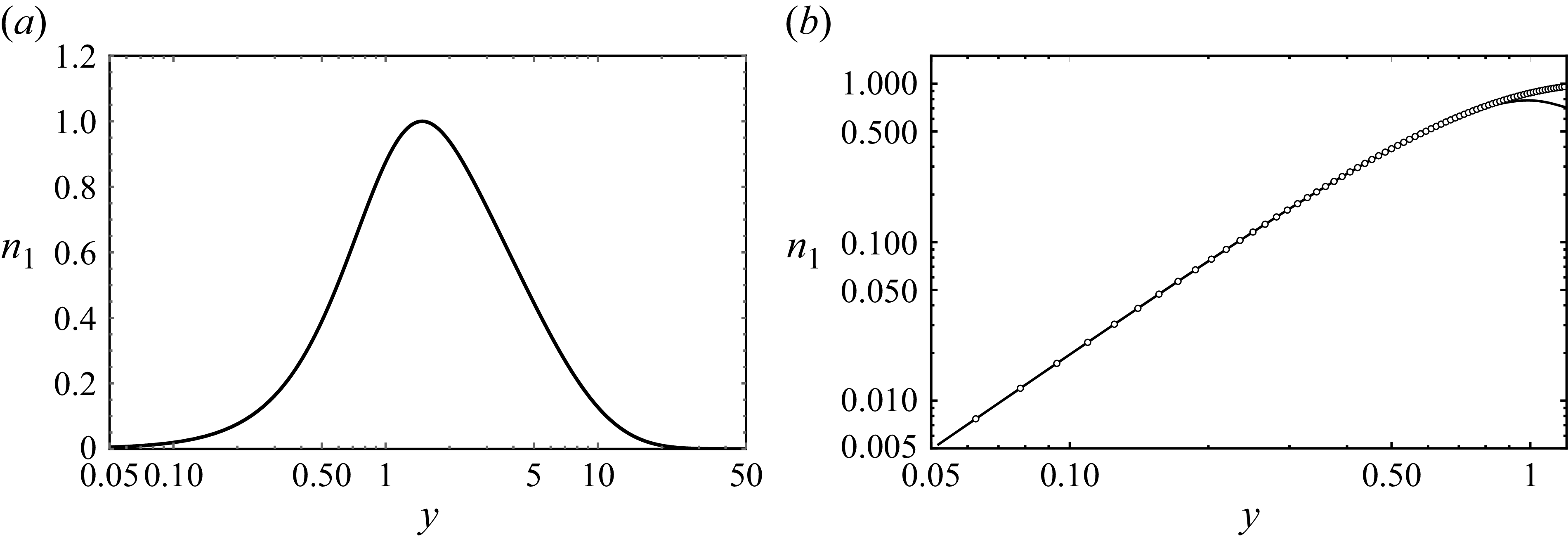
 k=1
 y=0
 ymax=50
 M=3200

 n1′
 n1′′
 n1′′′
 n1′′′′
 y

 A
 y≈12.03125
 k=1
 ymax=50
 M=3200

 cmin2
 k
 cmin2
 k
 ν
 ν>0

 k=0.5,0.75,1.0,1.5,5,10
 n1
 S~1

 k=2
 t=5.658
 n1/2=|ψ|
 y=0.7031
 192×256
 128×128
 0⩽x⩽2π
 10−4

 k=2
 ϵ=0.02
 t=5.658
 n1/2=|ψ|
 y=0.3125
 192×256
 128×128
 0⩽x⩽2π
 10−4

 Re[ψ(x,y)]
 k=2
 Im[ψ(x,y)]
 (ϵ,t)=(0.3,23.28)
 (J×M)=(128×128)

 Re[ψ],Im[ψ]
 (x,y)
 k=2
 ϵ=0.3
 Re[ψ]=0
 Im[ψ]=0
 t=9.84
 t=23.28
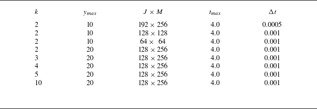
 ϵ=0.45

 |ψ(x,y)|
 t=0
 t=1.2
 t=2.8
 t=4.0
 (J×M)=(192×256)
 ymax=10

 |ψ(x,y)|
 (J×M)=(128×256)
 ϵ=0.45
 ymax=20.
 t=4.0.
 k=2
 k=3
 k=5
 k=10.
 J=128
 x
 k
 Jw≈128/k
 |ψ(x,y)|=0
 k

 Re[ψ|
 x
 t=2.8
 k=2
 ϵ=0.45
 y
 x=0
 y=0.3125,0.7813,1.7187
 Im[ψ|
 x
 t=2.8
 k=2
 ϵ=0.45
 y
 x=0
 y=0.3125,0.7813,1.7187
 (J×M,ymax)=(192×256,10)
 (J×M,ymax)=(128×256,20)
 (J×M,ymax)=(128×128,10)
 (J×M,ymax)=(64×64,10

 x
 |ψ|kx2
 y=0.89535
 k=2
 ϵ=0.45
 ymax=10
 t=2.36
 (192×256)
 (128×128)
 kx
 π
 2π
 k=2
 |ψ|2
 x
 (J×M)=(192×256)
 (J×M)=(128×128)

 Re[ψ],Im[ψ]
 (x,y)
 Re[ψ]=0
 Im[ψ]=0
 |ψ|
 t=1.8
 t=1.92
 t=2.1
 t=2.2
 y=0
 t≈1.92

 u(x,0,t)
 x
 t=1.7
 t=1.8
 t=2.0
 t=2.2
 Γ(t)/(4π)
 t
 k=2,ϵ=0.45
 Γ(t)
 t=1.992±0.002

 k=2,ϵ=0.45,t=1.92
 x=0.65,y=0
 x=0.65+π,y=0
 k=2,ϵ=0.45,t=4.0
 x=3.14,y=1.51
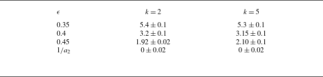
 tc
 ϵ
 k

 k
 a2
 −a4
 −b0
 x
 t=0
 a2=2.007,b0=−1.102
 k=2
 ϵ=0.3
 ϵ=0.45
 ϵ=1/a2−10−3

 y
 t
 y
 t
 y(t)=1.28(t−1.92)0.46
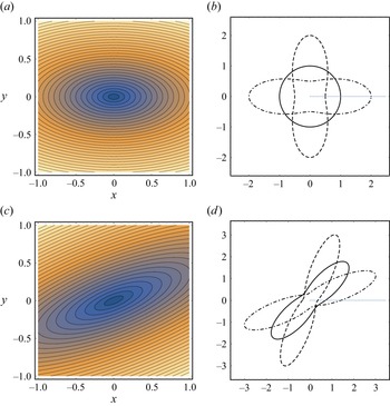
 n1/2=|ψ(x,y)|
 r=f(θ;K,α)
 uθ
 α=π/2
 K=2
 Γ=2π
 K=0.5
 K=1
 K=2
 α=5π/4
 a=K
 Γ=−2π
 K=0.5
 K=1
 K=2

 ΔE[ψ](t)=|(E[ψ](t)−E[ψ](0))/E[ψ](0)|
 t
 k=2,ϵ=0.45
 t=1.92

 A(θ,r)
 θ
 A(θ)<0
 r=0.9
 r=0.95
 r=0.99
 A(θ)>0
 r=1.1
 r=1.05
 r=1.01
 uRes(θ,r)
 θ



