1 Introduction
A remarkable aspect of turbulent flows is the organisation of coherent large-scale flow patterns superposed on small-scale fluctuations. Decomposing the turbulent flow into coherent flow structures and incoherent turbulence, allows us to focus on dynamically significant events (Hussain Reference Hussain1986). Such decomposition is usually performed either in terms of predetermined basis functions, like spatial Fourier decomposition (see, for instance, Das, Ghosal & Kumar Reference Das, Ghosal and Kumar2000, Chandra & Verma Reference Chandra and Verma2011), or in terms of basis functions extracted from the data, like proper orthogonal decomposition (POD) (see, for instance Bailon-Cuba, Emran & Schumacher Reference Bailon-Cuba, Emran and Schumacher2010, Podvin & Sergent Reference Podvin and Sergent2015, Reference Podvin and Sergent2017, Faranda, Podvin & Sergent Reference Faranda, Podvin and Sergent2019), dynamic mode decomposition (DMD) (Schmid Reference Schmid2010; Horn & Schmid Reference Horn and Schmid2017) or Koopman eigenfunction analysis (Giannakis et al. Reference Giannakis, Kolchinskaya, Krasnov and Schumacher2018). From this perspective, the coherent structures correspond to a combination of various such modes. In many instances, different configurations for the large-scale flows coexist and the system rapidly switches from one configuration to the other. Let us mention polarity switches in the Earth’s magnetic field or inside the dynamo laboratory experiments (Wicht, Stellmach & Harder Reference Wicht, Stellmach and Harder2009; Valet et al. Reference Valet, Fournier, Courtillot and Herrero-Bervera2012; Fauve et al. Reference Fauve, Herault, Michel and Pétrélis2017), or flow reversals inside decaying and stochastically forced two-dimensional turbulence in the presence of rigid walls (Molenaar, Clercx & Van Heijst Reference Molenaar, Clercx and Van Heijst2004; Van Heijst, Clercx & Molenaar Reference Van Heijst, Clercx and Molenaar2006). In this regard, flow reversals result from the nonlinear interactions between modes.
In turbulent Rayleigh–Bénard (RB) convection, flow reversals are also observed where the large-scale circulation (LSC), commonly referred to as the wind of turbulence, changes sign intermittently (Kadanoff Reference Kadanoff2001; Niemela et al. Reference Niemela, Skrbek, Sreenivasan and Donnelly2001; Sreenivasan, Bershadskii & Niemela Reference Sreenivasan, Bershadskii and Niemela2002). The structure of the LSC and the nature of its variations depend on the geometry of the container (Grossmann & Lohse Reference Grossmann and Lohse2003; Xi & Xia Reference Xi and Xia2008b ; van der Poel, Stevens & Lohse Reference van der Poel, Stevens and Lohse2011). In cylindrical RB cells, the LSC is subject to erratic reorientations of its vertical circulating plane by means of two different mechanisms: a constant azimuthal meandering and a momentary decline of the flow magnitude called cessation. Both mechanisms may lead to a change in the direction of the flow circulation, either by half a revolution of the LSC plane around the cylinder axis (a rotation-led reversal) or by a LSC restart after cessation in the same vertical plane but in the opposite direction (cessation-led reversal) (Brown, Nikolaenko & Ahlers Reference Brown, Nikolaenko and Ahlers2005; Xi, Zhou & Xia Reference Xi, Zhou and Xia2006). Reorientations by cessation are far more rare than those caused by azimuthal rotation. In turn, cessation-led reversals represent only a tiny part of cessations, all the angular changes after cessation having the same probability (Brown & Ahlers Reference Brown and Ahlers2006; Xi & Xia Reference Xi and Xia2008a ). In cubic RB cells, the LSC plane tends to align to the diagonals of the cell and sometimes changes its orientation through azimuthal rotation. Little or no evidence of cessation-led reversal has been mentioned in the literature (Bai, Ji & Brown Reference Bai, Ji and Brown2016; Foroozani et al. Reference Foroozani, Niemela, Armenio and Sreenivasan2017).
There are different ways to focus on the cessation-type events. One may hamper the azimuthal meandering by slightly tilting the convection cell, or prevent it by restricting the experimental configuration to slim (or quasi-two-dimensional) rectangular cells (Sugiyama et al.
Reference Sugiyama, Ni, Stevens, Chan, Zhou, Xi, Sun, Grossmann, Xia and Lohse2010; Vasilev & Frick Reference Vasilev and Frick2011). However, a strong dependence of the reversal dynamics on cell aspect ratio has been noticed in quasi-two-dimensional cells (Ni, Huang & Xia Reference Ni, Huang and Xia2015). Another possibility is to consider two-dimensional (2-D) direct numerical simulations (DNS) (Sugiyama et al.
Reference Sugiyama, Ni, Stevens, Chan, Zhou, Xi, Sun, Grossmann, Xia and Lohse2010; Chandra & Verma Reference Chandra and Verma2011, Reference Chandra and Verma2013; Petschel et al.
Reference Petschel, Wilczek, Breuer, Friedrich and Hansen2011; Podvin & Sergent Reference Podvin and Sergent2015, Reference Podvin and Sergent2017). This approach is interesting for different reasons. First, Sugiyama et al. (Reference Sugiyama, Ni, Stevens, Chan, Zhou, Xi, Sun, Grossmann, Xia and Lohse2010) used 2-D DNS to identify a region in the
 $(Ra,Pr)$
parameter space in which consecutive reversal events are observed, in good qualitative agreement with experimental observations. For this range of parameters, the LSC flow inside a square cell is mainly composed of a large diagonal roll and two counter-rotating corner rolls. As pointed out by Sugiyama et al. (Reference Sugiyama, Ni, Stevens, Chan, Zhou, Xi, Sun, Grossmann, Xia and Lohse2010), Chandra & Verma (Reference Chandra and Verma2013), in 2-D reversals the LSC is temporarily replaced by a quadrupolar mode during the transition. A second flow regime has been observed intermittently in 2-D DNS inside the same range of parameters. It is mainly composed either of two counter-rotating horizontally stacked rolls or two vertically stacked rolls (Podvin & Sergent Reference Podvin and Sergent2015). In the following, we refer to these regimes as the regime of consecutive reversals (CR) and the regime of extended cessations (EC), respectively. The intermittent switching between the CR and EC regimes features a rich dynamical behaviour. Second, two-dimensional (or quasi-2-D RB) flows may also be observed in practical configurations, such as those coupling turbulent convection with a strong magnetic field in typical fusion reactor conditions (Zhang & Zikanov Reference Zhang and Zikanov2015). Third, compared to 3-D DNS, 2-D DNS have a lower computational cost, thus giving access to long-term statistics.
Due to the wide range of involved temporal scales, the large-scale spatio-temporal dynamics of the CR and EC regimes is far from being completely described. In a previous work (Castillo-Castellanos, Sergent & Rossi Reference Castillo-Castellanos, Sergent and Rossi2016), we applied an amplitude-based filter to separate the CR and EC regimes. For the CR regime, a time-rescaling technique based on a well-defined characteristic time scale (the time between consecutive reversals) was combined with an ensemble average to investigate the energetics of flow reversals observed in long-term 2-D DNS data. This technique was previously used for reversals of geomagnetic fields (Valet et al. Reference Valet, Fournier, Courtillot and Herrero-Bervera2012; Lhuillier, Hulot & Gallet Reference Lhuillier, Hulot and Gallet2013). Using several hundred realisations of flow reversals, we followed the evolution of the global kinetic and available potential energies (as proposed by Winters et al. (Reference Winters, Lombard, Riley and D’Asaro1995), Hughes, Gayen & Griffiths (Reference Hughes, Gayen and Griffiths2013)), which led to the identification of a generic reversal mechanism which includes a long phase of LSC strength weakening (called accumulation) preceding a rapid transition (called release) and a rebound. This process shares common features with observations in cylindrical RB cells (Xi & Xia Reference Xi and Xia2008a ), as well as with geomagnetic reversals (Valet et al. Reference Valet, Fournier, Courtillot and Herrero-Bervera2012). In comparison, cessations are much less described, in particular regarding representative flow dynamics. In cylindrical cells, it is commonly admitted that reorientations by cessation (including cessation-led reversals) follow Poissonian statistics (Brown et al. Reference Brown, Nikolaenko and Ahlers2005; Brown & Ahlers Reference Brown and Ahlers2006; Xi & Xia Reference Xi and Xia2008a ). However, only a few selected instantaneous flow patterns are given (Xi & Xia Reference Xi and Xia2008b ). Additionally, a decoherence of the LSC has also been mentioned (Xi & Xia Reference Xi and Xia2007).
In the present paper, our objective is to separately characterise the spatio-temporal dynamics of the consecutive reversal and extended cessation regimes in a 2-D square cavity using the POD approach. First, as previously mentioned, some similarities between flows in a 2-D square cell and in a 3-D cylinder have been identified in the literature (Xi & Xia Reference Xi and Xia2008a ). Connections are based on phases observed in the generic reversal cycle proposed in Castillo-Castellanos et al. (Reference Castillo-Castellanos, Sergent and Rossi2016). This deterministic feature may appear paradoxical with respect to the well-known stochastic features of 3-D reversals. This is one of the points we try to elucidate: we reanalyse the 2-D flows in order to determine if only a part of flow in the CR regime may follow Poissonian statistics despite the existence of a generic reversal cycle. This question demands identification of the leading POD modes on the data subset corresponding to the CR regime before characterising the statistics of the waiting times of each POD mode. This leads us to reinterpret the generic reversal cycle in terms of POD mode dynamics. By applying the same methodology to the EC regime, we recover the expected Poissonian dynamics of cessations described in cylinders. However we seek to identify typical coherent dynamical events in this regime (specifically by distinguishing weak reversals from actual cessations). The total time periods related to the EC regime represent only a small part of the complete time series, and no clear characteristic time can be identified. Thus we cannot apply the previously used time rescaling leading to the identification of a generic mechanism. A specific methodology is consequently necessary to obtain some kind of classification into the spatio-temporal dynamics. This is performed by first identifying POD dynamical modes in the EC subset, and then analysing the paths followed by the system in POD state space using statistical approaches. In particular, we use a cluster-based analysis of the POD phase diagrams as proposed by Kaiser et al. (Reference Kaiser, Noack, Cordier, Spohn, Segond, Abel, Daviller, Östh, Krajnovi and Niven2014), to identify typical dynamical events whatever their probability of occurrence. These are described in terms of representative flow patterns (the centroids of the clusters) and time spent by the system inside each type of event.
The paper is organised as follows. Section 2 introduces the model equations, their numerical implementation and the POD approach. In § 3, we present the criterion used to separate the CR and EC regimes and introduce the data sampling for POD. The following sections explore the differences between both regimes: § 4 focuses on the spatial structure of coherent modes, § 5 on their temporal evolution, while § 6 and § 7 introduce and apply cluster analysis to analyse the interactions between competing modes for the CR and EC regimes, respectively. In § 8, we follow the energy contained inside different modes and the residence times in clusters as a function of
 $Ra$
. This provides a simplified description of the various flow regimes observed. Finally, we summarise our results in § 9.
2 Model equations and analysis tools
2.1 Physical configuration and governing equations
Consider a fluid contained in a square cell, cooled at the top with constant temperature
 $T_{top}$
and heated at the bottom with constant temperature
 $T_{bot}>T_{top}$
. The flow equations are based on the Boussinesq approximation. The flow is defined by the Rayleigh and Prandtl numbers
 $$\begin{eqnarray}\displaystyle Ra\equiv \frac{g\unicode[STIX]{x1D6FD}H^{3}(T_{bot}-T_{top})}{\unicode[STIX]{x1D705}\unicode[STIX]{x1D708}},\quad Pr\equiv \frac{\unicode[STIX]{x1D708}}{\unicode[STIX]{x1D705}}, & & \displaystyle\end{eqnarray}$$
where
 $g$
denotes gravity,
 $H$
the cell height and
 $\unicode[STIX]{x1D6FD}$
,
 $\unicode[STIX]{x1D705}$
,
 $\unicode[STIX]{x1D708}$
are respectively volumetric thermal expansion, thermal diffusivity and kinematic viscosity coefficients. As far as notations are concerned, variables
 $x$
(respectively
 $u$
) and
 $y$
(respectively
 $v$
) stand for the horizontal and vertical directions (respectively velocities). Coordinate vector
 $\boldsymbol{x}=(x,y)$
is equal to
 $(0,0)$
at the cavity centre. One introduces the reduced temperature
 $\unicode[STIX]{x1D703}(\boldsymbol{x},t)\equiv (T-T_{0})/(T_{bot}-T_{top})$
, with
 $T_{0}\equiv (T_{bot}+T_{top})/2$
. Given a field
 $a(\boldsymbol{x},t)$
, quantity
 $\overline{a}(\boldsymbol{x})$
(respectively
 $\unicode[STIX]{x1D70E}(a)(\boldsymbol{x})$
) denotes the time-averaged value (respectively standard deviation) computed using the complete long-term time series. Moreover
 $\langle a\rangle (t)$
stands for the volume average of
 $a(\boldsymbol{x},t)$
over the fluid domain.
Based on the cell height
 $H$
as characteristic length scale and
 $(\unicode[STIX]{x1D705}/H)Ra^{0.5}$
as characteristic velocity scale (one obtained from a balance between the friction and buoyancy forces, equivalent to the free-fall velocity divided by
 $Pr^{0.5}$
) the dimensionless velocity
 $\boldsymbol{u}=(u,v)$
and reduced temperature
 $\unicode[STIX]{x1D703}$
satisfy the dimensionless system of equations
 $$\begin{eqnarray}\displaystyle \left.\begin{array}{@{}c@{}}\unicode[STIX]{x1D735}\boldsymbol{\cdot }\boldsymbol{u}=0,\\ \unicode[STIX]{x2202}_{t}\boldsymbol{u}+\unicode[STIX]{x1D735}\boldsymbol{\cdot }[\boldsymbol{u}\otimes \boldsymbol{u}]=-\unicode[STIX]{x1D735}p+PrRa^{-0.5}\unicode[STIX]{x1D6FB}^{2}\boldsymbol{u}+Pr\unicode[STIX]{x1D703}\boldsymbol{e}_{y},\\ \unicode[STIX]{x2202}_{t}\unicode[STIX]{x1D703}+\unicode[STIX]{x1D735}\boldsymbol{\cdot }[\boldsymbol{u}\unicode[STIX]{x1D703}]=Ra^{-0.5}\unicode[STIX]{x1D6FB}^{2}\unicode[STIX]{x1D703}.\end{array}\right\} & & \displaystyle\end{eqnarray}$$
A no-slip condition for the velocity field is ensured on walls. On top (respectively bottom) walls, one imposes
 $\unicode[STIX]{x1D703}=-0.5$
(respectively
 $\unicode[STIX]{x1D703}=0.5$
) while adiabaticity
 $\unicode[STIX]{x2202}_{x}\unicode[STIX]{x1D703}=0$
is satisfied on side walls. From now on, all quantities are written in dimensionless form only.
2.2 DNS: parameter range and numerical method
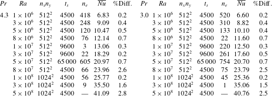
Simulation parameters:
 $Ra$
and
 $Pr$
, number of grid points
 $n_{x}n_{y}$
, simulation length
 $t_{s}$
in convective time units and number of events
 $n_{e}$
where the global angular momentum
 $A_{2D}(t)$
(defined in (3.1)) changes sign during the simulation length. Numerical convergence of the Nusselt number: average Nusselt number and maximum relative difference between different definitions, see text.

The values of
 $(Ra,Pr)$
used for direct numerical simulations covers the transition to a turbulent flow regime where reversals have been reported (Sugiyama et al.
Reference Sugiyama, Ni, Stevens, Chan, Zhou, Xi, Sun, Grossmann, Xia and Lohse2010):
 $Ra=10^{6}-5\times 10^{8}$
for
 $Pr=3$
and
 $Pr=4.3$
. Sections 3–7 are mainly focused on
 $Ra=5\times 10^{7}$
, while § 8 explores the different dynamical regimes observed as function of
 $Ra$
. Whenever both
 $Pr$
display similar results, we present in detail only those for
 $Pr=3$
. The length of the simulations range from 4500 to 65 000 convective time units as to observe an adequate number of reversals of the LSC (see table 1).
Time integration of the governing equations (2.2) is performed through a second-order semi-implicit scheme. It combines a staggered in time discretisation of the velocity and scalar fields with an implicit treatment of the diffusion terms and the Bell–Colella–Glaz advection scheme (Bell, Colella & Glaz Reference Bell, Colella and Glaz1989) for the nonlinear terms. Details of this method can be found in Popinet (Reference Popinet2003, Reference Popinet2009). The time step is variable and verifies the Courant–Friedrichs–Lewy condition CFL
 ${<}0.5$
. Incompressibility is imposed by a projection method. Numerical implementation is done using Basilisk (Popinet Reference Popinet2015). The code has been validated and verified for Rayleigh–Bénard convection in Castillo-Castellanos et al. (Reference Castillo-Castellanos, Sergent and Rossi2016). Simulations are performed using the finite volume method on a regular Cartesian centred grid with 512 or 1024 points in each direction. We verify the spatial resolution by evaluating the numerical convergence of time-averaged Nusselt numbers obtained by different methods: integrated over the top and bottom plates, over the volume and derived from exact relations to the viscous and thermal dissipation rates (Shraiman & Siggia Reference Shraiman and Siggia1990). In general, these values converge within 2 % of the average Nusselt number, see table 1.
2.3 Mode extraction using proper orthogonal decomposition
Proper orthogonal decomposition (Lumley Reference Lumley, Yaglom and Tatarski1967) is a statistical technique which provides a representation of a spatio-temporal vector field
 $\unicode[STIX]{x1D74D}(\boldsymbol{x},t)$
as the superposition of a enumeration of space-dependent structures or empirical eigenfunctions
 $\unicode[STIX]{x1D753}_{k}(\boldsymbol{x})$
,
 $k\geqslant 1$
, the amplitude of which
 $\unicode[STIX]{x1D6FC}_{k}$
varies in time,
 $$\begin{eqnarray}\displaystyle \unicode[STIX]{x1D74D}(\boldsymbol{x},t)=\mathop{\sum }_{k=1}^{\infty }\unicode[STIX]{x1D6FC}_{k}(t)\unicode[STIX]{x1D753}_{k}(\boldsymbol{x}). & & \displaystyle\end{eqnarray}$$
Here, the field consists of the joint velocity and temperature fields
 $\unicode[STIX]{x1D74D}=\{\boldsymbol{u},\unicode[STIX]{x1D6FE}\unicode[STIX]{x1D703}\}$
, where
 $\unicode[STIX]{x1D6FE}$
is an arbitrary rescaling factor here taken equal to 1 (the influence of
 $\unicode[STIX]{x1D6FE}$
was studied in Podvin & Sergent (Reference Podvin and Sergent2015)).
The empirical eigenfunctions constitute a hierarchy of patterns most likely to be observed in the simulation and they are solutions of the eigenvalue problem
 $$\begin{eqnarray}\displaystyle \int \unicode[STIX]{x1D64D}(\boldsymbol{x},\boldsymbol{x}^{\prime })\unicode[STIX]{x1D753}_{k}(\boldsymbol{x}^{\prime })\,\text{d}\boldsymbol{x}^{\prime }=\unicode[STIX]{x1D706}_{k}\unicode[STIX]{x1D753}_{k}(\boldsymbol{x}), & & \displaystyle\end{eqnarray}$$
where
 $\unicode[STIX]{x1D64D}(\boldsymbol{x},\boldsymbol{x}^{\prime })\equiv (1/N)\sum _{n=1}^{N}\unicode[STIX]{x1D74D}(\boldsymbol{x},t_{n})\unicode[STIX]{x1D74D}(\boldsymbol{x}^{\prime },t_{n})$
is the spatial autocorrelation tensor computed from
 $N$
snapshots obtained at times
 $t_{i},i=1\ldots N$
. By construction the eigenfunctions are orthogonal (see Holmes et al. (Reference Holmes, Lumley, Berkooz and Rowley2012) for more details). It can be shown that the problem can be reformulated into what is called the method of snapshots, following Sirovich (Reference Sirovich1987), as
 $$\begin{eqnarray}\displaystyle C_{mn}\unicode[STIX]{x1D6FC}_{n}^{k}=\unicode[STIX]{x1D706}_{k}\unicode[STIX]{x1D6FC}_{m}^{k},\quad \text{with }C_{mn}\equiv \langle \unicode[STIX]{x1D74D}(\boldsymbol{x},t_{m})\unicode[STIX]{x1D74D}(\boldsymbol{x},t_{n})\rangle . & & \displaystyle\end{eqnarray}$$
The amplitude
 $\unicode[STIX]{x1D6FC}_{n}^{k}=\unicode[STIX]{x1D6FC}^{k}(t_{n})$
represents the amplitude of mode
 $k$
at time
 $t_{n}$
. By construction the amplitudes are uncorrelated, and if the eigenfunctions are normalised, we have
 $\overline{\unicode[STIX]{x1D6FC}_{j}\unicode[STIX]{x1D6FC}_{k}}=\unicode[STIX]{x1D6FF}_{jk}\unicode[STIX]{x1D706}_{k}$
,
 $\unicode[STIX]{x1D6FF}_{jk}$
being the Kronecker symbol. The eigenvalues
 $\unicode[STIX]{x1D706}_{k},k\geqslant 1$
represent the average contribution of mode
 $k$
to the total energy of the vector field
 $E_{comb}\equiv \langle \overline{\unicode[STIX]{x1D703}^{2}+\boldsymbol{u}^{2}}\rangle =\sum _{k=1}^{\infty }\unicode[STIX]{x1D706}_{k}$
and can be ordered
 $\unicode[STIX]{x1D706}_{1}\geqslant \unicode[STIX]{x1D706}_{2}\geqslant \cdots \unicode[STIX]{x1D706}_{k}$
.
The idea is then to superimpose the small set of dominant modes identified by the decomposition to build an approximation to the actual flow field (in other words the flow is replaced by its projection onto the first few most energetic modes). We note that the relationship between empirical eigenfunctions and the standard definition of a coherent structure is not entirely straightforward, as empirical eigenfunctions correspond to linear combinations of individual realisations of the flow over the full spatial domain
 $$\begin{eqnarray}\displaystyle \unicode[STIX]{x1D753}_{k}(\boldsymbol{x})=\mathop{\sum }_{n=1}^{N}\unicode[STIX]{x1D6FC}_{k}(t_{n})\unicode[STIX]{x1D74D}(\boldsymbol{x},t_{n}), & & \displaystyle\end{eqnarray}$$
while standard definitions of coherent structures (such as the corner rolls) are typically local in space. More on this can be found in Podvin & Sergent (Reference Podvin and Sergent2017).
For this system, we identify the following symmetry operators which leave the governing equations invariant: a reflection symmetry
 $\mathbb{S}_{x}$
with respect to the vertical axis (
 $x=0$
),
 $$\begin{eqnarray}\displaystyle \left[\begin{array}{@{}c@{}}u(x,y)\\ v(x,y)\\ \unicode[STIX]{x1D703}(x,y)\end{array}\right]\overset{\mathbb{S}_{x}}{\longrightarrow }\left[\begin{array}{@{}c@{}}-u(-x,y)\\ v(-x,y)\\ \unicode[STIX]{x1D703}(-x,y)\end{array}\right], & & \displaystyle\end{eqnarray}$$
and a reflection symmetry
 $\mathbb{S}_{y}$
with respect to the horizontal axis (
 $y=0$
).
 $$\begin{eqnarray}\displaystyle \left[\begin{array}{@{}c@{}}u(x,y)\\ v(x,y)\\ \unicode[STIX]{x1D703}(x,y)\end{array}\right]\overset{\mathbb{S}_{y}}{\longrightarrow }\left[\begin{array}{@{}c@{}}u(x,-y)\\ -v(x,-y)\\ -\unicode[STIX]{x1D703}(x,-y)\end{array}\right]. & & \displaystyle\end{eqnarray}$$
The combination of both
 $R_{\unicode[STIX]{x03C0}}=\mathbb{S}_{x}\circ \mathbb{S}_{y}=\mathbb{S}_{y}\circ \mathbb{S}_{x}$
represents the centrosymmetry.
 $$\begin{eqnarray}\displaystyle \left[\begin{array}{@{}c@{}}u(x,y)\\ v(x,y)\\ \unicode[STIX]{x1D703}(x,y)\end{array}\right]\overset{R_{\unicode[STIX]{x03C0}}}{\longrightarrow }\left[\begin{array}{@{}c@{}}-u(-x,-y)\\ -v(-x,-y)\\ -\unicode[STIX]{x1D703}(-x,-y)\end{array}\right], & & \displaystyle\end{eqnarray}$$
which in addition to the identity form a symmetry group (Podvin & Sergent Reference Podvin and Sergent2015). In this work, we extract a set of POD modes
 $M$
. In the next paragraph, we show that each mode
 $M$
possesses symmetries related to elements
 $\mathbb{E}$
of the symmetry group. Each mode can be symmetric, i.e.
 $\mathbb{E}M=M$
, or antisymmetric, i.e.
 $\mathbb{E}M=M$
. In keeping the naming scheme proposed by Podvin & Sergent (Reference Podvin and Sergent2017), we introduce the following notations for coherent modes: (i) two modes
 $Q$
and
 $Q^{\ast }$
, which are symmetric with respect to all the elements of the group; (ii) two modes
 $L$
and
 $L^{\ast }$
, which are symmetric with respect to
 $R_{\unicode[STIX]{x03C0}}$
, but antisymmetric with respect to
 $\mathbb{S}_{x}$
and
 $\mathbb{S}_{y}$
; and (iii) two modes
 $S$
and
 $S^{\ast }$
, also known as symmetry-breaking modes, which are antisymmetric with respect to
 $R_{\unicode[STIX]{x03C0}}$
. However, mode
 $S$
is symmetric with respect to
 $\mathbb{S}_{y}$
and antisymmetric with respect to
 $\mathbb{S}_{x}$
, while mode
 $S^{\ast }$
has the opposite symmetries (see table 2).
To validate our approach, POD was applied a set of 1200 snapshots for (
 $Ra=5\times 10^{7}$
,
 $Pr=4.3$
). Snapshots were taken every 5 convective time units (t.u.) from the complete series. Using a longer series or a smaller sampling time did not affect results, giving some confidence in the robustness of our mode extraction. Results are in good agreement with Podvin & Sergent (Reference Podvin and Sergent2017), see figure 1.
Definition of modes based on symmetry properties. In each case, we indicate whether the mode is symmetric (S) or antisymmetric (AS) with respect to
 $\mathbb{S}_{x}$
,
 $\mathbb{S}_{y}$
, and
 $R_{\unicode[STIX]{x03C0}}$
.

Leading POD modes obtained from the complete series for
 $Ra=5\times 10^{7}$
and
 $Pr=4.3$
. For each figure, colour corresponds to the temperature modes
 $\unicode[STIX]{x1D719}_{k}^{\unicode[STIX]{x1D703}}$
(a) and to the streamfunction of the velocity modes
 $(\unicode[STIX]{x1D719}_{k}^{u},\unicode[STIX]{x1D719}_{k}^{v})$
(b). Streamlines are also presented in the bottom row with dashed lines for negative streamfunction values.

3 Data processing: identification of regimes and conditional sampling
3.1 Identification of the two flow regimes
(a) Time evolution of
 $A_{2D}(t)$
scaled by
 $\overline{|A_{2D}|}$
for
 $(Ra=5\times 10^{7},Pr=3)$
. The threshold separating the CR and EC regimes set to
 $A_{thres}=\overline{|A_{2D}|}+\unicode[STIX]{x1D70E}(|A_{2D}|)$
is shown in red. White areas correspond to CR, while grey areas correspond to EC. Panel (b) (respectively (c)) displays snapshots taken inside the CR (respectively EC) regime. Colour indicates temperature field
 $\unicode[STIX]{x1D703}(\boldsymbol{x},t)$
and lines are streamlines (negative values shown in dashed).

For the range of
 $(Ra,Pr)$
considered, two different dynamical regimes have been identified by following the global angular momentum
 $$\begin{eqnarray}\displaystyle A_{2D}(t)\equiv -\frac{1}{2}\int \boldsymbol{x}^{2}\unicode[STIX]{x1D714}(\boldsymbol{x},t)\,\text{d}\boldsymbol{x},\quad \text{ with }\unicode[STIX]{x1D714}(\boldsymbol{x},t)=\unicode[STIX]{x2202}_{x}v-\unicode[STIX]{x2202}_{y}u & & \displaystyle\end{eqnarray}$$
as a function of time (figure 2
a). Indeed, this quantity is a measure of the organised rotation around the centre of the cavity, i.e. the strength of the LSC (Molenaar et al.
Reference Molenaar, Clercx and Van Heijst2004). A criterion based on the amplitude of
 $A_{2D}$
was proposed to discriminate the two regimes (Podvin & Sergent Reference Podvin and Sergent2015; Castillo-Castellanos et al.
Reference Castillo-Castellanos, Sergent and Rossi2016). If
 $|A_{2D}|>A_{thres}$
(here set to
 $A_{thres}=\overline{|A_{2D}|}+\unicode[STIX]{x1D70E}(|A_{2D}|)$
) during the interval between two consecutive sign changes in
 $A_{2D}$
, then the time interval is assigned to the regime of consecutive reversals (CR), corresponding to white areas in figure 2(a). A time interval where such threshold is not reached can be of two kinds: weak reversals if only one consecutive sign change is observed, and a cessation of the LSC otherwise. For simplicity, both kinds are assigned to the regime of extended cessations (EC), corresponding to grey areas in figure 2(a). On the one hand, consecutive reversals are characterised by alternating positive and negative plateaus in
 $A_{2D}$
. Positive (respectively negative) plateaus are associated with a large counter-clockwise (respectively clockwise) diagonal roll with two corner rolls (see figure 2
b). On the other hand, extended cessations are characterised by a more erratic dynamics and by the absence of a central vortex (see figure 2
c).
3.2 Conditional sampling for POD
Conditional sampling allows us to distinguish and provide quantitative information about interesting spatial and/or temporal regions of a turbulent flow (Antonia Reference Antonia1981). Here, we use the aforementioned criterion to separate our data into two subsets: a first one which corresponds to the CR regime only and a second one which excludes this regime, leaving mostly the EC regime. The idea is now to apply a POD analysis to each subset separately and investigate in detail the dynamics of each regime. In §§ 4–7, we focus on the values
 $(Ra=5\times 10^{7},Pr=3)$
and
 $(Ra=5\times 10^{7},Pr=4.3)$
since the system displays in that two cases an intermittency between the CR and EC regimes. For reference, at
 $(Ra=5\times 10^{7},Pr=3)$
(respectively
 $(Ra=5\times 10^{7},Pr=4.3)$
) the probability of being inside the CR regime is 79.6 % (respectively 83.0 %) of the complete series. It is thus possible to highlight the different roles played by the large-scale modes from different viewpoints. These observations will be used in § 8 to follow the large-scale flow dynamics over a wider range of
 $Ra$
numbers.
For
 $(Ra=5\times 10^{7},Pr=3)$
, the CR subset is restricted to 108 flow reversals, corresponding to 1521 snapshots taken every 4 convective time units. The sampling frequency of snapshots has been adjusted to ensure the different phases of the flow reversals are represented and the number of snapshots was progressively increased until the convergence of POD modes is reached. The EC subset is composed of 1500 snapshots taken every convective time unit. The sampling frequency was increased due to the generally faster dynamics and short duration of this regime. For this regime it was more difficult to obtain converged POD modes and small differences are still observed when considering different sets of snapshots. For
 $(Ra=5\times 10^{7},Pr=4.3)$
the CR subset is composed of 100 reversals, corresponding to 3157 snapshots taken every 4 time units, while the EC subset is composed of 3800 snapshots taken every time unit.
4 Comparison of the spatial structures extracted from each regime
For
 $(Ra=5\times 10^{7},Pr=3)$
and
 $(Ra=5\times 10^{7},Pr=4.3)$
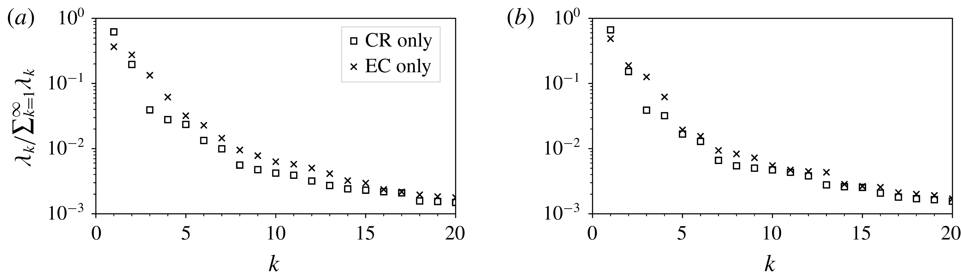
, and both CR and EC subsets, the POD spectra exhibit at least two decades of decay between modes
 $k=1$
and
 $k=20$
(figure 3). The two first modes of the CR regime represent approximately 80 % of the combined energy
 $E_{comb}$
, with an additional 10 % contained inside modes
 $k=3$
to 7 for
 $Pr=3$
(respectively modes
 $k=3$
to 6 for
 $Pr=4.3$
). In comparison, the first two and six modes of the EC regime represent 70 % and 86 % of
 $E_{comb}$
, respectively. Generally EC modes
 $k=2$
to
 $20$
are more energetic than their CR counterparts, indicating a stronger competition between POD modes for the EC subset. In §§ 4.1 and 4.2, we study only on the six most energetic POD modes for each regime. In the following and whenever there is no ambiguity, we refer to the amplitude
 $\unicode[STIX]{x1D6FC}_{k}(t)$
of the mode
 $k$
as the mode itself. For instance if
 $k=1$
mode is a mode
 $Q$
,
 $\unicode[STIX]{x1D6FC}_{1}$
is written as
 $Q$
.
Conditional POD analysis of the CR and EC subsets. Normalised eigenvalues for the first 20 modes for
 $Ra=5\times 10^{7}$
for (a)
 $Pr=3.0$
and (b)
 $Pr=4.3$
.

4.1 Leading POD modes inside the regime of ‘consecutive reversals’ (CR)
Leading POD modes of the CR subset obtained for
 $Ra=5\times 10^{7}$
and
 $Pr=3.0$
. For each panel, colour corresponds to the temperature modes
 $\unicode[STIX]{x1D719}_{k}^{\unicode[STIX]{x1D703}}$
(a) and to the streamfunction of the velocity modes
 $(\unicode[STIX]{x1D719}_{k}^{u},\unicode[STIX]{x1D719}_{k}^{v})$
(b). Streamlines are also presented in the bottom row with dashed lines for negative streamfunction values.

Figure 4 displays the POD modes extracted from the CR subset for
 $(Ra=5\times 10^{7},Pr=3)$
. Each mode displays a clear symmetry. Mode
 $k=1$
corresponds to
 $L$
, associated with a single-roll mode with small recirculation cells in the four corners. In the following, this mode will be used as a marker of the strength of the LSC. Mode
 $k=2$
corresponds to
 $Q$
, associated with a four-roll mode and to the mean temperature field. Indeed, a linear combination of centrosymmetric modes
 $L$
and
 $Q$
roughly corresponds to the LSC with added corner rolls, the most recognisable flow structure of the CR regime. Mode
 $k=3$
corresponds to
 $L^{\ast }$
, composed of three vertically stacked rolls;
 $k=4$
to mode
 $S$
, composed of two vertically stacked rolls, analogous to the short-lived double-roll mode observed in cylindrical cells (Xi & Xia Reference Xi and Xia2008b
). Mode
 $k=5$
corresponds to mode
 $Q^{\ast }$
, similar to mode
 $Q$
, but with four additional rolls carrying cold (respectively hot) fluid close to the bottom (respectively top) plate; and finally
 $k=6$
corresponds to mode
 $S^{\ast }$
, composed of two horizontally stacked rolls. For
 $(Ra=5\times 10^{7},Pr=4.3)$
one obtains a similar set of POD modes but with modes
 $k=3$
and
 $k=4$
interchanged.
4.2 Leading POD modes inside the regime of ‘extended cessations’ (EC)
Most energetic POD modes of the EC subset obtained for
 $Ra=5\times 10^{7}$
and
 $Pr=3.0$
. Temperature and velocity modes are displayed as in figure 4.

Figure 5 displays POD modes extracted from the EC subset for
 $(Ra=5\times 10^{7},Pr=3)$
. Such modes are reminiscent of those extracted from the CR subset:
 $k=1$
is similar to the symmetry-breaking mode
 $S$
, but the temperature field suggests this mode is a linear combination of modes
 $S$
and
 $Q$
. Similarly,
 $k=2$
can be seen as a linear combination of centrosymmetric modes
 $L$
and
 $L^{\ast }$
with
 $LL^{\ast }>0$
, and corresponds to a vortex detached from the top and bottom plates (Podvin & Sergent Reference Podvin and Sergent2017). Both leading modes have comparable energetic contents (figure 3). Unlike the CR regime, the EC regime displays a strong competition between modes with different symmetries. Modes
 $k=3$
,
 $k=4$
and
 $k=5$
, are reminiscent of modes
 $Q$
,
 $S^{\ast }$
and
 $Q^{\ast }$
, respectively, while
 $k=6$
is a new mode specific to the EC regime. The latter one is composed of two co-rotating vortices surrounded by six smaller counter-rotating rolls. A similar set of POD modes is obtained for
 $(Ra=5\times 10^{7},Pr=4.3)$
.
Given the similarities between the modes extracted from EC and CR subsets (the sole exception being the mode
 $k=6$
of the EC regime), we conclude that both subsets are accurately represented by the same set of coherent spatial structures. This suggests that differences between the CR and EC regimes concern the time evolution of modal amplitudes. In the following sections, we hence project the complete time series into the set of modes extracted from the CR regime as to compare the temporal evolution of the modal amplitudes for both regimes.
5 Comparison of temporal evolution in the CR and EC regimes
We analyse here the temporal evolution in both regimes and focus on the coherent or stochastic nature of the dynamics of each POD mode.
5.1 General temporal evolution and probability density functions of modal amplitudes
Scaled amplitudes
 $\unicode[STIX]{x1D6FC}_{k}(t)/\overline{|L|}$
and the scaled angular impulse
 $A_{2D}/\overline{|A_{2D}|}$
for
 $(Ra=5\times 10^{7},Pr=3)$
. White (respectively shaded) regions belong to the CR (respectively EC) subset. Red solid lines on the top figure pinpoint the threshold separating the CR and EC subsets. The presented time series correspond to approximately
 $1/16$
of the total simulation length.

Probability distributions of the scaled amplitudes
 $\unicode[STIX]{x1D6FC}_{k}(t)/\overline{|L|}$
for
 $(Ra=5\times 10^{7},Pr=3)$
. Probability distribution functions inside the CR regime are displayed in blue, while conditional PDFs inside EC regime are displayed in red.

Let us project the fields
 $\unicode[STIX]{x1D74D}(\boldsymbol{x},t)=(\unicode[STIX]{x1D703},u,v)$
into the set of POD modes
 $\unicode[STIX]{x1D719}_{k}(\boldsymbol{x})$
extracted from the CR subset to obtain the modal amplitudes
 $\unicode[STIX]{x1D6FC}_{k}(t)$
. For simplicity, these amplitudes are then scaled by the common factor
 $1/\overline{|L|}$
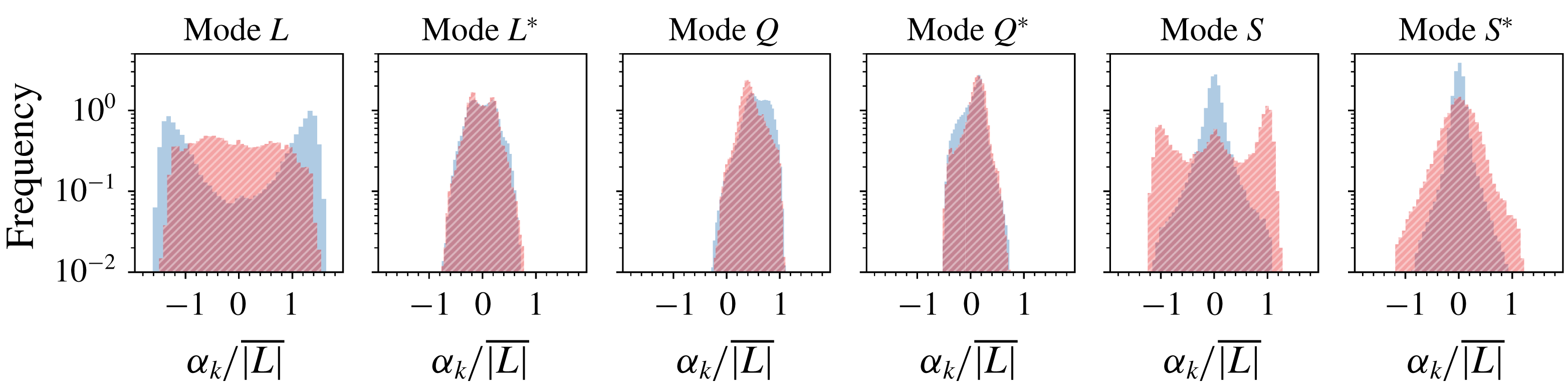
. Figure 6 displays their time evolution, and figure 7 their corresponding probability distribution functions (PDFs). A different behaviour is observed for the CR and EC regimes.
During the CR regime (white areas), the dominant mode
 $L$
alternates between positive and negative plateaus. Both
 $A_{2D}$
(shown in green) and
 $L$
are very well correlated and are considered as excellent indicators of the presence of flow reversals. As observed by Podvin & Sergent (Reference Podvin and Sergent2017), the time evolution of mode
 $L^{\ast }$
is different for positive and negative values of
 $L$
. Modes
 $S$
and
 $S^{\ast }$
display positive and negative peaks during transitions, but otherwise fluctuate around zero. Mode
 $Q$
increases progressively during the plateaus and suddenly drops during transitions, while
 $Q^{\ast }$
is centred around zero and displays the opposite behaviour. As far as the PDFs are concerned, modes
 $L$
and
 $L^{\ast }$
display a bimodal distribution, modes
 $S$
and
 $S^{\ast }$
, a double exponential distribution, which is almost symmetric. On the contrary, modes
 $Q$
and
 $Q^{\ast }$
have skewed probability distributions. This behaviour can be explained as follows. If a set of amplitudes
 $M(t)\equiv \{L,L^{\ast },Q,Q^{\ast },S,S^{\ast }\}$
is obtained by the governing equations, then
 $\mathbb{S}_{x}M$
,
 $\mathbb{S}_{y}M$
, and
 $R_{\unicode[STIX]{x03C0}}M$
are also data sets associated with these governing equations. Furthermore, contrary to modes
 $Q$
and
 $Q^{\ast }$
which are symmetric under operators
 $\mathbb{S}_{x}$
,
 $\mathbb{S}_{y}$
and
 $R_{\unicode[STIX]{x03C0}}$
, the modes
 $\{L,L^{\ast },S,S^{\ast }\}$
are changed into their opposite by the action of at least one of these operators (see table 2). Consequently their PDFs are expected to symmetric with respect to zero. This is not completely the case in figure 7 due to limited number of records.
During the EC regime (shaded areas), the dominant mode
 $S$
is characterised by positive and negative plateaus and its PDF takes the form of a symmetric bimodal distribution. This is analogous to the evolution of mode
 $L$
during the CR regime. Mode
 $S$
is therefore a good marker for this regime. Mode
 $S^{\ast }$
becomes more energetic than in the CR regime, but does not exhibit such clear plateaus. The time evolution of the other POD modes is also modified by the change of regime: modes
 $\{L,L^{\ast }\}$
are found to oscillate around zero or may display smaller positive and negative plateaus, while
 $\{Q,Q^{\ast }\}$
fluctuate around a non-null positive value.
For the above symmetry considerations, the PDFs of modes
 $\{L,L^{\ast },S,S^{\ast }\}$
are symmetric with respect to zero. As such, these modes are prone to exhibit a reversing dynamics (see figure 6), and the dynamics of each mode is similar for its positive and negative values. By contrast, the PDFs of modes
 $Q$
and
 $Q^{\ast }$
are skewed: mode
 $Q$
does not reverse, whereas
 $Q^{\ast }$
does change sign, but evolves differently for its positive and negative values. Consequently, in order to characterise the temporal dynamics of each regime more precisely, we study the process governing the reversing modes
 $\{L,L^{\ast },S,S^{\ast }\}$
.
5.2 Distribution of waiting times for reversing POD modes
To characterise the reversal process of modes
 $\{L,L^{\ast },S,S^{\ast }\}$
, we compute for each such mode the waiting time
 $\unicode[STIX]{x1D70F}$
between consecutive sign changes and evaluate its probability distribution
 $P(\unicode[STIX]{x1D70F})$
. The quantity
 $h(\unicode[STIX]{x1D70F})\,\text{d}\unicode[STIX]{x1D70F}$
where
 $h(\unicode[STIX]{x1D70F})\equiv P(\unicode[STIX]{x1D70F})/(1-\int _{0}^{\unicode[STIX]{x1D70F}}P(\unicode[STIX]{x1D70F}^{\prime })\,\text{d}\unicode[STIX]{x1D70F}^{\prime })$
, stands for the probability of the occurrence of another reversal inside time interval
 $[\unicode[STIX]{x1D70F},\unicode[STIX]{x1D70F}+\text{d}\unicode[STIX]{x1D70F}]$
where
 $\unicode[STIX]{x1D70F}$
is defined as the time elapsed since the last reversal. The probability distributions
 $P(\unicode[STIX]{x1D70F})$
and
 $h(\unicode[STIX]{x1D70F})$
are often employed for polarity reversals of the Earth’s magnetic field. Polarity changes are typically assumed to originate from a general renewal process, in which reversals are independent from one another (see, for instance Merrill, McElhinny & McFadden Reference Merrill, McElhinny and McFadden1998; Lhuillier et al.
Reference Lhuillier, Hulot and Gallet2013). To verify whether or not the independence hypothesis is correct, the probability distribution
 $P(\unicode[STIX]{x1D70F})$
is compared to a gamma distribution
 $$\begin{eqnarray}\displaystyle P(\unicode[STIX]{x1D70F})=\left(\frac{k}{m}\right)^{k}\frac{\unicode[STIX]{x1D70F}^{k-1}}{\unicode[STIX]{x1D6E4}(k)}\exp \left(-k\frac{\unicode[STIX]{x1D70F}}{m}\right),\quad \text{with }\unicode[STIX]{x1D6E4}(k)=\int _{0}^{\infty }x^{k-1}\exp (-x)\,\text{d}x, & & \displaystyle\end{eqnarray}$$
where
 $m=\overline{\unicode[STIX]{x1D70F}}$
denotes the mean value of
 $\unicode[STIX]{x1D70F}$
and the shape parameter
 $k$
provides the standard deviation
 $m/\sqrt{k}$
. For a gamma distribution,
 $h$
reaches a constant
 $\lim _{\unicode[STIX]{x1D70F}\rightarrow \infty }h(\unicode[STIX]{x1D70F})=k/m$
at long time intervals (McFadden & Merrill Reference McFadden and Merrill1986). When
 $k=1$
, the probability
 $h$
is found always constant
 $h(\unicode[STIX]{x1D70F})=1/m$
. This exponential distribution is interpreted as a lack of memory of the system: reversals are thus generated by a Poisson process characterised by an affine profile in a log plot, i.e.
 $\log P(\unicode[STIX]{x1D70F})=-(\unicode[STIX]{x1D70F}/m)-\log m$
. On the contrary, a memory effect appears when
 $k\neq 1$
: on the one hand, for
 $k>1$
the distribution is such that
 $\lim _{\unicode[STIX]{x1D70F}\rightarrow 0}h(\unicode[STIX]{x1D70F})=0$
, indicating a temporary inhibition of future reversal events at short times. On the other hand, for
 $k<1$
,
 $h$
diverges for
 $\unicode[STIX]{x1D70F}\rightarrow 0$
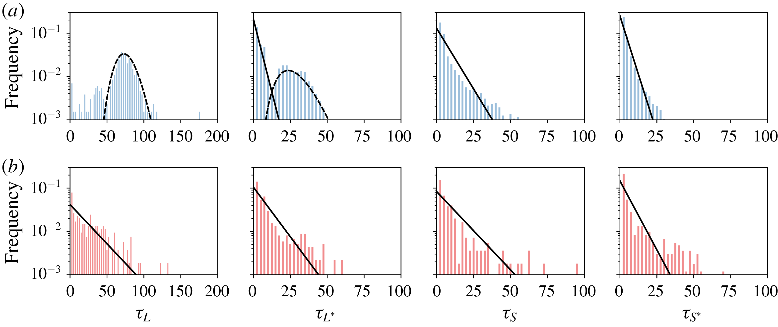
indicating an encouragement at short times. Figure 8 displays the distribution of waiting times from the CR and EC subsets for
 $(Ra=5\times 10^{7},Pr=3)$
. Probability distribution functions are compared either to gamma distributions with
 $k>1$
(dashed lines) or to exponential distributions (solid lines) using the parameters listed in table 3. To illustrate the goodness of each fit, table 3 also includes the quantity
 $R^{2}\equiv 1-\sum _{bin}e^{2}/\sum _{bin}P_{hist}^{2}$
where
 $P_{hist}$
is the estimated density distribution using histograms and
 $e$
is the error between the fit and the histogram. In this context, a value
 $R^{2}=1$
indicates that the gamma distribution perfectly fits the histogram.
Distribution of waiting times
 $\unicode[STIX]{x1D70F}_{M}$
of modes
 $M=\{L,L^{\ast },S,S^{\ast }\}$
for
 $(Ra=5\times 10^{7},Pr=3)$
. (a) Displays the CR regime and (b) the EC regime. Probability distribution functions are obtained using histograms with fixed bins of 2.5 t.u. width. Exponential (solid) and gamma distributions with
 $k\neq 1$
(dashed) are drawn using parameters from table 3.

(a) CR subset and (b) EC subset for (
 $Ra=5\times 10^{7},Pr=3$
). Values
 $k$
and
 $m$
define the fit of the probability distributions of waiting times
 $\unicode[STIX]{x1D70F}_{M}$
to either exponential (in that case
 $k$
is set to 1) or gamma distributions with
 $k\neq 1$
. The coefficient
 $R^{2}$
quantifies the goodness of the fit (see text). Finally
 $n$
denotes the number of events where a mode changes signs.
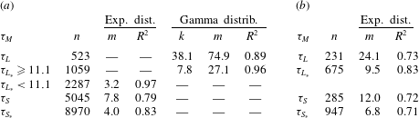
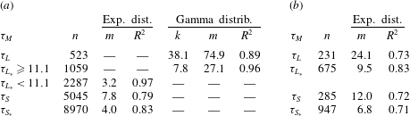
For the EC subset, the distribution of waiting times for all reversing modes fits reasonably well to exponential distributions (figure 8), so indicating a Poisson-like dynamics for all modes studied: the cessation regime seems to be composed of memoryless events. In the EC regime, the lack of memory was identified previously by Brown et al. (Reference Brown, Nikolaenko and Ahlers2005), Brown & Ahlers (Reference Brown and Ahlers2006) in three-dimensional flows. Our POD analysis simply confirms that all modes have Poissonian statistics for waiting times and no memory in the EC regime.
For the CR subset, the distributions of
 $\unicode[STIX]{x1D70F}_{S}$
, and
 $\unicode[STIX]{x1D70F}_{S^{\ast }}$
also fit well exponential distributions. By contrast, the distributions
 $P(\unicode[STIX]{x1D70F}_{L})$
for mode
 $L$
are fitted to gamma distributions with
 $k=38$
, with large dispersion and a peak value around
 $\unicode[STIX]{x1D70F}_{L}=70$
t.u., several times longer than the large eddy turnover time
 $t_{E}\approx 3.5$
t.u. The leading mode
 $L$
thus strongly deviates from Poissonian statistics, suggesting that the system keeps a form of memory of the preceding reversals. This highlights the coherent behaviour of the large-scale structures specific to the CR regime. The distribution of
 $\unicode[STIX]{x1D70F}_{L^{\ast }}$
displays elements of the exponential and gamma distributions: if one separates the values less than a cutoff value around 11 t.u. (this value is comparable to the duration of the transition from a positive to negative plateau for
 $A_{2D}$
, see Castillo-Castellanos et al. (Reference Castillo-Castellanos, Sergent and Rossi2016)). The shorter time scales
 $\unicode[STIX]{x1D70F}_{L\ast }<11$
follow an exponential distribution, whereas the longer time scales
 $\unicode[STIX]{x1D70F}_{L\ast }\geqslant 11$
are governed by a gamma distribution with
 $k=9$
for
 $Pr=3$
(respectively
 $k=8$
for
 $Pr=4.3$
). In this respect, the distribution of
 $\unicode[STIX]{x1D70F}_{L^{\ast }}$
reflects the interplay between long-term coherent dynamics and short-term random fluctuations typical of this regime.
As a final remark, evaluating the PDFs of the waiting times considering both subsets at once would mask the more coherent nature of the CR regime.
5.3 Generic reversal in the CR regime
The time coherence displayed by some POD modes (
 $L$
and
 $L^{\ast }$
) in the CR regime can be further studied by revisiting the statistical approach proposed in Castillo-Castellanos et al. (Reference Castillo-Castellanos, Sergent and Rossi2016). This procedure extracts a generic reversal cycle from an ensemble of realisations. First, one identifies the set of consecutive times
 $t_{i}$
at which a marker of reversal changes sign. Here, we use the amplitude
 $L(t)$
as the marker of the reversal. Consider a time interval
 $[t_{i},t_{i+1}]$
in which the marker
 $L(t)\geqslant 0$
; a quantity
 $a(t)$
in this interval is represented in the re-scaled time
 $t_{o}=(t-t_{i+1})/(t_{i+1}-t_{i})$
, so that
 $a(t_{o}|t_{o}\in [-1,0])$
. Conversely, for an interval
 $[t_{i},t_{i+1}]$
in which the marker
 $L(t)\leqslant 0$
,
 $a(t)$
is represented in the re-scaled time
 $t_{o}=(t-t_{i})/(t_{i+1}-t_{i})$
, so that
 $a(t_{o}|t_{o}\in [0,1])$
. The ensemble average over the rescaled curves represents the evolution of
 $a(t_{o})$
during a generic reversal in the interval
 $t_{o}\in [-1,1]$
. This treatment may exhibit the presence of a dynamical path in
 $a(t)$
that repeats over the ensemble of realisations. In contrast, if
 $a(t)$
displays random fluctuations throughout the reversal cycle, its generic curve is flat.
Bivariate histograms of the global kinetic energy
 $E_{kin}$
, available potential energy
 $E_{apot}$
and of the modal amplitudes as function of re-scaled time
 $t_{o}$
during a generic reversal for
 $(Ra=5\times 10^{7},Pr=3)$
. Generic curves are displayed in solid lines, while dotted lines indicate one standard deviation. Colour intensity indicates the probability density (here shown for the blue phase, but equivalent for the other colours), while the colour indicates the three phases of a generic reversal in energetic viewpoint: accumulation (blue), release (orange) and acceleration (green). A precursory region to the flow reversal is enclosed between vertical blue lines, see text.

The idea is to use this averaging procedure on the POD mode amplitudes to characterise (in the statistical sense) their dynamical evolution and to connect this back to the generic reversal mechanism proposed by Castillo-Castellanos et al. (Reference Castillo-Castellanos, Sergent and Rossi2016). In said work, the marker of reversal was the global angular impulse
 $A_{2D}(t)$
while quantity
 $a(t)$
was the global angular impulse itself or the global kinetic energy
 $E_{kin}(t)\equiv \int \frac{1}{2}\boldsymbol{u}^{2}\,\text{d}\boldsymbol{x}$
, or else the available potential energy
 $E_{apot}(t)$
(for a precise definition of
 $E_{apot}(t)$
, see Winters et al. (Reference Winters, Lombard, Riley and D’Asaro1995), Hughes et al. (Reference Hughes, Gayen and Griffiths2013)). From this viewpoint, the generic reversal mechanism is composed of 3 consecutive phases. First, an accumulation phase characterised by a progressive decrease in
 $E_{kin}$
as
 $E_{apot}$
builds up inside growing corner rolls. This is followed by a release phase where energy is exchanged from
 $E_{apot}$
to
 $E_{kin}$
, complete with a rebound. Last, the acceleration phase where
 $E_{kin}$
increases while
 $E_{apot}$
remains fairly constant during the recovery of the LSC. Additionally, a precursory region was identified, indicating the transition from a LSC dominant to a corner-roll dominant flow.
Now, let us consider the amplitudes of the POD modes during a generic reversal (see figure 9). For the sake of comparison with the energy analysis presented in Castillo-Castellanos et al. (Reference Castillo-Castellanos, Sergent and Rossi2016) the accumulation phase is identified in figure 9, by a blue colour, the release phase by an orange colour and the acceleration phase by a green colour. Finally the two vertical lines indicate the position of the precursory region.
Modes
 $\{S,S^{\ast }\}$
do not display any particularly coherent shape (flat generic curves with larger amplitudes observed from the precursory region until the end of the acceleration phase). In contrast, the modes
 $\{L,L^{\ast },Q,Q^{\ast }\}$
show some very coherent dynamical patterns. Modes
 $\{L,L^{\ast }\}$
carry the flow reversal. Given the spatial structure of
 $\{L,L^{\ast }\}$
, the main circulation is reinforced when both modes have amplitudes with opposite signs. At the beginning of the accumulation phase,
 $L$
and
 $L^{\ast }$
have opposite signs. Consider the case with
 $L(t_{o})>0$
and
 $L^{\ast }(t_{o})<0$
(the opposite case being equivalent). During the accumulation phase,
 $L^{\ast }$
increases progressively and becomes positive, thus weakening the circulation along the upper and lower boundary layers. A peak in
 $L^{\ast }>0$
coincides with the change in sign of mode
 $L$
. Modes
 $\{Q,Q^{\ast }\}$
carry the thermal energy. Mode
 $Q$
progressively increases during the plateau state, then suddenly drops, before returning to its initial value, reminiscent of the generic reversal of
 $E_{apot}$
. This could be expected: by construction, the contribution to
 $E_{apot}$
from modes antisymmetric with respect to
 $\mathbb{S}_{x}$
is null, thus leaving symmetric modes
 $\{Q,Q^{\ast }\}$
as the main carriers of
 $E_{apot}$
since
 $S^{\ast }$
is negligible. It can be shown by computation that contributions to
 $E_{apot}$
from the spatial eigenfunction related to mode
 $Q$
and
 $Q^{\ast }$
are positive, which can be understood in terms of thermal stratification, see figure 4. As a function of time, mode
 $Q^{\ast }$
is centred around zero and is anticorrelated to
 $Q$
. During the generic cycle, the contribution to
 $E_{apot}$
of mode
 $Q^{\ast }$
compensates in part that of
 $Q$
. Finally, note that modes
 $Q^{\ast }$
and
 $L^{\ast }$
, change signs close to the precursory region. This coincides with a change in slope for
 $E_{apot}$
. Our observations place the precursory time at approximately 75 % of
 $t_{o}$
(or 56 t.u.). By switching signs, these modes, because of their spatial structure, mark the detachment of the LSC from the top/bottom plates and the progressive redistribution of thermal energy towards the bulk which precedes the flow reversal.
For the case
 $(Ra=5\times 10^{7},Pr=4.3)$
, similar trends are found. The change in sign of modes
 $L^{\ast }$
and
 $Q^{\ast }$
is observed around 72 % of
 $t_{o}$
(or 89 t.u.). The most noticeable difference with respect to
 $Pr=3$
concerns the rebound, which is less intense, and the evolution of
 $E_{apot}$
, which displays a steeper slope inside the precursory region. Our observations are also in good agreement with the limit cycle obtained from the 5-mode model by Podvin & Sergent (Reference Podvin and Sergent2017). The precursor event and the precursor duration as defined in the same work are also recovered in the generic cycle of POD modes.
6 Exploring the CR regime using the cluster-based analysis
One way to explore further the differences between the CR and EC regimes is to study the statistical correlations between modes. However, it is not an easy matter to exhibit connections between the complete set of modes at the same time. To achieve this goal, we provide a drastically simplified description of the spatio-temporal dynamics in terms of network dynamics with
 $K$
representative states. The temporal dynamics is then reduced to two elements: the trajectories followed between these
 $K$
points and the residence time, which is the time spent inside each point. To define this network, we seek a decomposition of a six-dimensional phase space made up of the POD amplitudes recorded every
 $\unicode[STIX]{x1D6FF}t$
into a finite set of clusters of points
 $(c_{k},k=1,\ldots ,K)$
. Each cluster
 $c_{k}$
is characterised by a centroid
 $\unicode[STIX]{x1D741}_{k}$
, i.e. the average of the ensemble of six-dimensional points in
 $c_{k}$
. Centroids become the points of the network, each associated with a representative spatial pattern, which may be seen as the most common superposition of POD modes inside the cluster. In the following and whenever there is no ambiguity, we refer to the cluster
 $c_{k}$
corresponding to the centroid
 $\unicode[STIX]{x1D707}_{k}$
by the centroid
 $\unicode[STIX]{x1D707}_{k}$
itself.
An adequate sampling frequency
 $\unicode[STIX]{x1D6FF}t$
and a large number of records are key to obtain correct results. For the present work, the POD amplitudes
 $\unicode[STIX]{x1D6FC}_{k}(t)$
are taken every
 $\unicode[STIX]{x1D6FF}t=0.05$
time units. Additionally, we apply the operators
 $\mathbb{S}_{x}$
,
 $\mathbb{S}_{y}$
, and
 $R_{\unicode[STIX]{x03C0}}$
(defined in (2.7) to (2.9)) to the amplitudes
 $\unicode[STIX]{x1D6FC}_{k}$
to increase the number of records since such a data set is a possible one for the dynamics. This greatly facilitates the interpretation by enforcing the natural symmetries of the system. The partitioning of the phase space is done using the
 $K$
-means clustering algorithm, as described in Kaiser et al. (Reference Kaiser, Noack, Cordier, Spohn, Segond, Abel, Daviller, Östh, Krajnovi and Niven2014). The algorithm is tasked to find a partition that minimises the total within-cluster variance, i.e. the squared distance between points inside a cluster and the corresponding centroid. This requires fixing the number
 $K$
of clusters. Further details are provided in appendix A.
In the present section we validate our approach on the CR regime. The study of the EC regime is presented in § 7.
6.1 Flow patterns associated with cluster centroids in the CR regime
Flow patterns corresponding to the
 $K=12$
cluster centroids extracted from the CR subset for
 $(Ra=5\times 10^{7},Pr=3)$
. Colour indicates the temperature field, and lines correspond to the streamlines (negative values of streamfunction are dashed). The five groups are identified by a different colour of the bottom ruler.

For
 $(Ra=5\times 10^{7},Pr=3)$
, partitioning the CR subset using
 $K=12$
clusters is found to be satisfactory (see appendix A). These clusters are organised in 5 groups
 $(G_{k}^{cr},k=1,\ldots ,5)$
, each associated with a different colour in figures 10 to 12:
(i) Three groups
 $G_{k}^{cr}$
,
$(k=1,2,3)$
, each characterised by two clusters which are
$\mathbb{S}_{x}$
and
$\mathbb{S}_{y}$
antisymmetric. The cluster centroids are denoted
$\{\unicode[STIX]{x1D707}_{k}^{+},\unicode[STIX]{x1D707}_{k}^{-}\}$
, superscripts indicating the sign in mode
$L$
. Colours are green, yellow and blue, respectively.
(ii) A single group
$G_{4}^{cr}$
with four clusters. Centroids are denoted
$\{\unicode[STIX]{x1D707}_{4}^{++},\unicode[STIX]{x1D707}_{4}^{+-},\unicode[STIX]{x1D707}_{4}^{-+}$
,
$\unicode[STIX]{x1D707}_{4}^{--}\}$
, superscripts indicating the quadrant in the (
$L,S$
) plane. Colour is red.(iii) A single group
$G_{5}^{cr}$
with two clusters which are
$\mathbb{S}_{y}$
-symmetric. The cluster centroids are denoted
$\{\unicode[STIX]{x1D707}_{5}^{+},\unicode[STIX]{x1D707}_{5}^{-}\}$
, superscripts indicating the sign in mode
$S$
. Colour is grey.


The flow patterns associated with each cluster centroid are displayed in figure 10. They indeed capture the underlying physics. For members of
 $G_{1}^{cr}$
(green),
 $G_{2}^{cr}$
(yellow) and
 $G_{3}^{cr}$
(blue), the flow pattern exhibits a large diagonal roll with counter-rotating corner rolls of different sizes, typical of the growth of corner rolls. For members of
 $G_{4}^{cr}$
(red) the flow pattern exhibits a central vortex partially detached from the top/bottom plates which is typical of the rearrangement of the LSC. Members of
 $G_{1}^{cr}$
to
 $G_{4}^{cr}$
can be easily recognised as rough approximations of the LSC during a generic reversal (see, for instance figure 7 in Castillo-Castellanos et al. (Reference Castillo-Castellanos, Sergent and Rossi2016)). For members of
 $G_{5}^{cr}$
(grey), the flow pattern corresponds to a vertically stacked double roll which forms an horizontal jet. A horizontal jet impacts one of the side walls along which two small corner rolls are placed, reminiscent of the leading mode of the EC regime (see figure 5). This flow pattern is predominantly observed during cessations (Podvin & Sergent Reference Podvin and Sergent2015).
6.2 Analysis of reversals in cluster space
Time series of the cluster
 $\unicode[STIX]{x1D707}_{k}$
visited at time
 $t$
and the corresponding amplitudes of modes
 $L$
,
 $Q$
and
 $S$
, during a series of particular flow reversals observed for
 $(Ra=5\times 10^{7},Pr=3)$
. Data points inside the EC subset correspond to the shaded areas, whereas data points from the CR subset are coloured to match the groups
 $G_{k}^{cr}$
, see colour code at the top part of the figure.

The simplified representation via clusters is also capable of retrieving the three phases of the reversal cycle (accumulation, release and acceleration). Figure 11 displays the clusters visited as a function of time shown alongside a time series of the amplitudes of modes
 $L$
,
 $Q$
and
 $S$
. The time series covers a series of standard flow reversals interspersed by two weak reversals, which are assigned to the EC subset and will be discussed in § 7. For all standard reversals, the clusters are almost always visited in the same sequence. Starting from a positive
 $L$
, the sequence
 $(\unicode[STIX]{x1D707}_{1}^{+},\unicode[STIX]{x1D707}_{2}^{+},\unicode[STIX]{x1D707}_{3}^{+})$
illustrates the growing corner rolls observed during the accumulation phase, where
 $\unicode[STIX]{x1D707}_{2}^{+}$
roughly corresponds to a precursory region identified in § 5.3. This is followed by a sequence
 $(\unicode[STIX]{x1D707}_{3}^{+},\unicode[STIX]{x1D707}_{3}^{-},\unicode[STIX]{x1D707}_{2}^{-})$
which splits into two branches (either
 $\unicode[STIX]{x1D707}_{4}^{--}$
or
 $\unicode[STIX]{x1D707}_{4}^{-+}$
) and corresponds to the beginning of the release phase (sign change in
 $L$
) leading to the rebound event. Finally, during the complex re-organisation process typical of the acceleration phase, the system alternates between different clusters (
 $\unicode[STIX]{x1D707}_{4}^{--}$
,
 $\unicode[STIX]{x1D707}_{1}^{-}$
,
 $\unicode[STIX]{x1D707}_{4}^{-+}$
), before eventually settling down on
 $\unicode[STIX]{x1D707}_{1}^{-}$
.
Figure 12 displays in the planes
 $(L,Q)$
and
 $(L,S)$
: (i) a random sample of data points coloured according to the corresponding cluster groups, (ii) the position of the cluster centroids and (iii) the generic reversal cycle from § 5.3. In these planes, all of the cluster centroids are located along the generic cycle with the exception of centroids
 $\{\unicode[STIX]{x1D707}_{5}^{+},\unicode[STIX]{x1D707}_{5}^{-}\}$
and centroids
 $\{\unicode[STIX]{x1D707}_{4}^{++},\unicode[STIX]{x1D707}_{4}^{+-},\unicode[STIX]{x1D707}_{4}^{-+},\unicode[STIX]{x1D707}_{4}^{--}\}$
. It is inside the
 $(L,S)$
plane that the two branches leading to the rebound event are best seen. Since both branches have equal probability of occurrence, by averaging over the ensemble of realisations, the generic cycle inevitably ‘smoothes out’ both branches. Consequently, cluster analysis is better suited to work whenever multiple transition paths are observed.
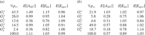
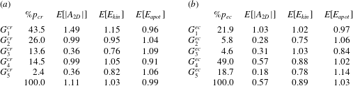
For each group
 $G_{k}^{cr}$
, we compute the residence time
 $\%p_{cr}$
, as well as the conditional average for different global quantities (table 4
a). The system spends 70 % of its time inside
 $G_{1}^{cr}$
and
 $G_{2}^{cr}$
, while it spends 14 % of its time inside
 $G_{3}^{cr}$
and
 $G_{4}^{cr}$
each. This is in good agreement with the duration of each phase of the generic reversal cycle with an energy viewpoint (Castillo-Castellanos et al.
Reference Castillo-Castellanos, Sergent and Rossi2016). The sequences described above are also consistent with the evolution of
 $A_{2D}$
,
 $E_{kin}$
, and
 $E_{apot}$
during a generic reversal. For instance, the sequence
 $(\unicode[STIX]{x1D707}_{1}^{+},\unicode[STIX]{x1D707}_{2}^{+},\unicode[STIX]{x1D707}_{3}^{+})$
displays a gradual increase of
 $E[E_{apot}]$
as in the accumulation phase. By contrast, the group
 $G_{5}^{cr}$
is only visited whenever deviations from standard reversals become important, like at the beginning and at the end of a series of consecutive reversals (see, for instance
 $t\sim 16\,200$
and
 $t\sim 16\,550$
in figure 11). For such events the residence time is always of a few per cent (table 4
a).
Phase diagram in the
 $(L,Q)$
and
 $(L,S)$
planes for
 $(Ra=5\times 10^{7},Pr=3)$
inside the CR subset. For reference, the generic reversal from § 5.3 is displayed in solid lines. Data points are coloured to match the groups
 $G_{k}^{cr}$
, see colour code at the top of the figure. Solid marks indicate the corresponding centroids.

Conditional averages over each of the groups extracted from the (a) CR and (b) EC regimes for
 $(Ra=5\times 10^{7},Pr=3)$
.
 $p_{cr}$
(respectively
 $p_{ec}$
) denotes the probability for the system to be inside
 $G_{k}^{cr}$
(respectively
 $G_{k}^{ec}$
) while
 $E[a]$
denotes the conditional average of
 $a(t)$
over a cluster normalised by the average
 $\overline{a}$
over the complete series.
7 Exploring the EC regime using the cluster-based analysis
In the previous section, we have shown that cluster analysis recovers the features of the CR regime obtained using the statistical method of § 5.3 and it is even able to obtain more detailed aspects. Here, the same cluster analysis explores the regime of extended cessations (EC), which is far less well understood. Note that the statistical method used in § 5.3 would be ineffective for the EC regime, since this method relies on the presence of a dominant time scale (the waiting time between consecutive reversals) to rescale time and extract a dynamical pattern from many realisations. Such dominant time scale has not been identified for the EC regime.
7.1 Flow patterns associated with the cluster centroids in the EC regime
For
 $(Ra=5\times 10^{7},Pr=3)$
, partitioning the EC subset using
 $K=11$
clusters is found to be satisfactory (see appendix A). For clarity, the centroids extracted from the EC subset are noted
 $\unicode[STIX]{x1D708}_{k}$
in order to differentiate the CR and EC subsets. These clusters are organised in 5 groups
 $(G_{k}^{ec},k=1,\ldots ,5)$
, each associated with a different colour in figures 14–16:
(i) A single group
$G_{1}^{ec}$
with two clusters which are
$\mathbb{S}_{x}$
and
$\mathbb{S}_{y}$
antisymmetric. Centroids are denoted
$\{\unicode[STIX]{x1D708}_{1}^{+},\unicode[STIX]{x1D708}_{1}^{-}\}$
, superscripts indicating the sign of mode
$L$
. Colour is green.(ii) A single group
$G_{2}^{ec}$
with a single cluster
$\{\unicode[STIX]{x1D708}_{2}\}$
which satisfies all the symmetries. Colour is yellow.(iii) A single group
$G_{3}^{ec}$
with two clusters which are
$\mathbb{S}_{x}$
-symmetric. The cluster centroids are denoted
$\{\unicode[STIX]{x1D708}_{3}^{+},\unicode[STIX]{x1D708}_{3}^{-}\}$
, superscripts indicating the sign of mode
$S^{\ast }$
. Colour is blue.(iv) A single group
$G_{4}^{ec}$
with four clusters. Centroids are denoted
$\{\unicode[STIX]{x1D708}_{4}^{++},\unicode[STIX]{x1D708}_{4}^{+-},\unicode[STIX]{x1D708}_{4}^{-+},\unicode[STIX]{x1D708}_{4}^{--}\}$
, superscripts indicating quadrant in the (
$L,S$
) plane. Colour is red.(v) A single group
$G_{5}^{ec}$
with two clusters which are
$\mathbb{S}_{y}$
-symmetric. The cluster centroids are denoted
$\{\unicode[STIX]{x1D708}_{5}^{+},\unicode[STIX]{x1D708}_{5}^{-}\}$
, superscripts indicating the sign of mode
$S$
. Colour is grey.





The flow patterns associated with each centroid are shown in figure 13. The large diagonal rolls are associated with
 $\unicode[STIX]{x1D708}_{1}^{+}$
and
 $\unicode[STIX]{x1D708}_{1}^{-}$
while a quadrupolar mode, commonly observed during standard reversals in the CR regime, is associated with
 $\unicode[STIX]{x1D708}_{2}$
. A horizontally stacked double-roll pattern with small corner rolls along the top or bottom plates is associated with
 $\unicode[STIX]{x1D708}_{3}^{+}$
and
 $\unicode[STIX]{x1D708}_{3}^{-}$
. For
 $\{\unicode[STIX]{x1D708}_{4}^{++},\unicode[STIX]{x1D708}_{4}^{+-},\unicode[STIX]{x1D708}_{4}^{-+},\unicode[STIX]{x1D708}_{4}^{--}\}$
the flow pattern corresponds to a large vortex squeezed between one small and one big corner roll, clearly reminiscent of that of
 $\{\unicode[STIX]{x1D707}_{4}^{++},\unicode[STIX]{x1D707}_{4}^{+-},\unicode[STIX]{x1D707}_{4}^{-+},\unicode[STIX]{x1D707}_{4}^{--}\}$
. Finally, a vertically stacked double-roll pattern with corner rolls along the left or right side walls, nearly identical to that of
 $\unicode[STIX]{x1D707}_{5}^{+}$
and
 $\unicode[STIX]{x1D707}_{5}^{-}$
, is associated with
 $\unicode[STIX]{x1D708}_{5}^{+}$
and
 $\unicode[STIX]{x1D708}_{5}^{-}$
.
Flow patterns corresponding to the 11 cluster centroids extracted from the EC subset for
 $(Ra=5\times 10^{7},Pr=3)$
. Colour indicates the temperature field, while lines correspond to streamlines (negative values of streamfunction are dashed). The five groups of centroids are identified by a different colour as shown at the bottom ruler of the figure.

7.2 A cluster space approach of cessations
For the EC regime, figure 14 displays the clusters visited as a function of time alongside a time series of modes
 $L$
,
 $Q$
and
 $S$
, as done previously in figure 11 for the CR regime. Similarly, figure 15 displays the phase diagrams in the
 $(L,S)$
and
 $(S,S^{\ast })$
planes, being the most relevant planes for the cessation dynamics.
First, note that data points in figure 15 are evenly distributed between the clusters inside groups
 $G_{1}^{ec}$
,
 $G_{4}^{ec}$
and
 $G_{5}^{ec}$
. This is confirmed by computing the residence time for each single cluster, which is at most 12 % and is consistent with table 4
b since the residence time
 $\%p_{ec}$
in each group is nearly proportional to the number of elements.
The cluster-based analysis discriminates between different kinds of dynamical events within the EC regime. Based on the sequence of clusters visited, one identifies two dynamics: weak reversals (windows in figure 14 containing
 $t\sim 8800$
and
 $t\sim 9300$
) and actual cessations of the LSC (the remaining windows). Weak reversals deviate from standard reversals in CR mainly because of a larger amplitude of mode
 $S$
. This is likely due to the asymmetric growth of corner rolls. During these events, data points are found to visit prominently the cluster group
 $G_{1}^{ec}$
and to a smaller degree the group
 $G_{4}^{ec}$
. At the beginning of each weak reversal, the system visits
 $G_{2}^{ec}$
, then
 $G_{1}^{ec}$
. It may then visit
 $G_{4}^{ec}$
and
 $G_{1}^{ec}$
through different paths.
Time series indicating the cluster
 $c_{k}^{ec}$
visited at time
 $t$
and the corresponding amplitudes of modes
 $L$
,
 $Q$
and
 $S$
, during a series of extended cessations interspersed by several periods of consecutive flow reversals for
 $(Ra=5\times 10^{7},Pr=3)$
. The EC subset corresponds to white areas. Data points from the EC subset are coloured to match the groups
 $G_{k}^{ec}$
, see colour code at the top part of the figure.

Phase diagram in the (
 $L,S$
) and (
 $L,S^{\ast }$
) planes for
 $(Ra=5\times 10^{7},Pr=3)$
inside the EC subset. Colour is used to identify each cluster group, see colour code at the top of the figure:
 $G_{1}^{ec}$
, and
 $G_{2}^{ec}$
predominantly associated with weak reversals, and
 $G_{3}^{ec}$
,
 $G_{4}^{ec}$
and
 $G_{5}^{ec}$
predominantly associated with extended cessations. Solid marks indicate the corresponding centroids.

At the beginning of every actual cessation, the system visits
 $G_{2}^{ec}$
, then
 $G_{1}^{ec}$
as for weak reversals. However, the situation is then dynamically quite different: mode
 $L$
oscillates around zero,
 $Q$
fluctuates around a nearly constant value, while
 $S$
displays a plateau sporadically interrupted by short excursions like the ones observed around
 $t\sim 8600$
,
 $t\sim 9100$
and
 $t\sim 9900$
in figure 14. On the
 $(L,S)$
and
 $(S,S^{\ast })$
planes, clusters
 $\{\unicode[STIX]{x1D708}_{4}^{-+},\unicode[STIX]{x1D708}_{5}^{+},\unicode[STIX]{x1D708}_{4}^{++}\}$
and
 $\{\unicode[STIX]{x1D708}_{4}^{--},\unicode[STIX]{x1D708}_{5}^{-},\unicode[STIX]{x1D708}_{4}^{-+}\}$
are found to be sufficiently close to one another to be considered as part of two attractive basins. This qualitative assessment can be confirmed by measuring the distance between centroids in the 6-D subspace. These basins precisely correspond to the actual cessations (plateau in mode
 $S$
, oscillation in
 $L$
). In trajectory terms, the system moves back and forth between three clusters inside the groups
 $G_{4}^{ec}$
and
 $G_{5}^{ec}$
, e.g.
 $\{\unicode[STIX]{x1D708}_{4}^{-+},\unicode[STIX]{x1D708}_{5}^{+},\unicode[STIX]{x1D708}_{4}^{++}\}$
and the short excursion of mode
 $S$
are through
 $G_{1}^{ec}$
,
 $G_{2}^{ec}$
and
 $G_{3}^{ec}$
before returning to one of the attractive basins. From the centroid patterns of figure 13, it can be inferred that the back and forth between
 $G_{4}^{ec}$
and
 $G_{5}^{ec}$
is related to the competition between two counter-rotating vertically stacked vortices, where the relative size is reflected on the sign of
 $L$
. This is observed in the snapshots presented in figures 16(a)–16(f). Oscillations in mode
 $L$
are physically related to a continuous push and shove motion between a large ascending plume and one descending along one of the side walls from which a horizontal jet is formed. Both plumes remain locked along the same side wall until the plateau in mode
 $S$
is disrupted during a short excursion. A short excursion is presented in figures 16(g)–16(l). This particular event is triggered by the weakening of the horizontal jet (figure 16
g) which favours the emergence of a quadrupolar pattern (figure 16
h). A new unstable pattern forms from the merging of vortices coming from opposite corners (figure 16
i). This new flow structure rotates until it eventually re-organises into a more stable vertically stacked double-roll pattern. The most commonly observed feature during the rotation of the unstable pattern is the brief passage of an intense plume through the centre of the cavity, which corresponds to the passage through
 $G_{3}^{ec}$
(figure 16
j). This rapid event is characterised by large fluctuations in mode
 $Q$
and a substantial increase (of approximately 40 %) in the global heat transfer. For such rapid events, the residence time is 4.6 % of the total EC subset, that is less than 1 % of the total simulation length (table 4
b).
It is remarkable how the attractive basins
 $\{\unicode[STIX]{x1D708}_{4}^{-+},\unicode[STIX]{x1D708}_{5}^{+},\unicode[STIX]{x1D708}_{4}^{++}\}$
and
 $\{\unicode[STIX]{x1D708}_{4}^{--},\unicode[STIX]{x1D708}_{5}^{-},\unicode[STIX]{x1D708}_{4}^{-+}\}$
are reminiscent of the double-roll modes (noted DMR1, DRM2 and DRM3 in Xi & Xia (Reference Xi and Xia2008b
)) observed inside cylindrical cells. For certain aspect ratios, the asymmetric configurations are more frequently observed than the symmetric one. This behaviour could be explained in part by a 3-D analogue of the push and shove motion described above.
Sequence of instantaneous fields observed during actual cessations for
 $(Ra=5\times 10^{7},Pr=3)$
. Colour indicates the temperature field
 $\unicode[STIX]{x1D703}(\boldsymbol{x},t)$
, lines are streamlines (negative streamfunction values in dashed). The coloured symbol of the top-right corner indicates the current cluster group (colour code at the top of the figure). Snapshots (a) to (f) are taken every 20 t.u. from
 $t=9090$
to
 $t=9190$
, whereas snapshots (g) to (l) are taken every 4 t.u. from
 $t=9882$
to
 $t=9902$
illustrating a short excursion.

8 Evolution of dynamical regimes as a function of Rayleigh number
For a given
 $Pr$
(in practice
 $Pr=4.3$
or
 $Pr=3$
), we take advantage of the POD and cluster-based analyses to find evidence of the dynamical flow regimes observed for different values of
 $Ra$
which cover the transition from a steady state to a turbulent flow regime. More precisely, a first study is based on the energetic content of the leading POD modes, a second on the residence time inside the different groups of clusters.
8.1 Energy contents of leading POD modes
To allow for a direct comparison between different
 $Ra$
, we use the modes
 $\unicode[STIX]{x1D753}_{k}$
extracted from the CR subset for
 $Ra=5\times 10^{7}$
for the
 $Pr$
considered (see § 4). For the different
 $Ra$
, we project the instantaneous velocity and temperature fields onto the six leading POD modes
 $\unicode[STIX]{x1D753}_{k}$
to obtain the set of amplitudes
 $(\unicode[STIX]{x1D6FC}_{k},k=1,\ldots ,6)$
. As in § 5, these modal amplitudes are then scaled by a common factor which is the value
 $1/\overline{|L|}$
for
 $Ra=5\times 10^{7}$
. Afterwards we compute
 $\overline{\unicode[STIX]{x1D6FC}_{k}\unicode[STIX]{x1D6FC}_{k}}$
, which is proportional to the part of the combined energy
 $E_{comb}$
contained inside mode
 $\unicode[STIX]{x1D753}_{k}$
(see § 2.3). We check the statistical convergence by splitting each series in half and comparing their mean values. For the values of
 $(Ra,Pr)$
considered, energy contained inside the six POD modes is somewhere between 80 and 95 % of the total energy
 $E_{comb}$
, while the maximum relative difference is about 2 %.
Let us focus on the energetic contents of the leading POD modes
 $L$
,
 $Q$
and
 $S$
(figure 17), which contain the main features of both the CR and EC regimes. As function of
 $Ra$
, we may identify different dynamical regimes: below mark i mode
 $L$
is dominant; between marks i and ii mode
 $Q$
is dominant; above ii mode
 $L$
becomes again dominant and remains so for larger values of
 $Ra$
; between iii and iv mode
 $S$
becomes comparable to
 $Q$
; above iv mode
 $S$
decreases with respect to modes
 $L$
and
 $Q$
. Note that, on the figure, we add a mark v which will be used in the next section. In the following, since both values of
 $Pr$
display similar trends, we focus on the case for
 $Pr=3$
.
Dynamical regimes as a function of
 $Ra$
for (a,c)
 $Pr=3$
and (b,d)
 $Pr=4.3$
. Marks i to v separate the different dynamical regimes (see text). (a,b) Display the rescaled values of
 $\overline{\unicode[STIX]{x1D6FC}_{k}\unicode[STIX]{x1D6FC}_{k}}$
, where
 $\unicode[STIX]{x1D6FC}_{k}$
is obtained by projection into CR modes for
 $Ra=5\times 10^{7}$
. Combined energy
 $\overline{E}_{comb}$
is shown for reference. (c,d) Display the probability
 $\%p_{ec}$
of the system being inside the cluster groups:
 $G_{1}^{ec}$
is predominantly associated with plateaus;
 $G_{2}^{ec}$
with transitions between plateaus;
 $G_{3}^{ec}$
with short excursions; and
 $G_{4}^{ec}$
and
 $G_{5}^{ec}$
with extended cessations.

Time series of the angular impulse
 $A_{2D}$
for
 $Pr=3$
and different
 $Ra$
illustrating the different flow regimes: (a) periodic reversals for
 $Ra=3\times 10^{5}$
, (b) chaotic reversals for
 $Ra=2\times 10^{6}$
, (c) appearance of long plateaus for
 $Ra=8\times 10^{6}$
, (d) flow reversals and extended cessations for
 $Ra=3\times 10^{7}$
, (e) flow reversals for
 $Ra=1\times 10^{8}$
and (f) long plateaus for
 $Ra=5\times 10^{8}$
.

In order to highlight the relation between the LSC dynamics and the energetic contents of POD modes, figure 18 displays a time series of
 $A_{2D}$
for different values of
 $Ra$
representing each dynamical regime. For values of
 $Ra$
between the onset of convection and mark i, a steady-state roll is observed. The jump of mode
 $Q$
around mark i coincides with the transition to unsteady flows. Region i–ii corresponds to continuous reversals of the LSC but without the accumulation phase, i.e. modes
 $Q$
and
 $L$
have the same dominant frequency and the plateaus in
 $A_{2D}$
are completely absent. Examples of this zone are a periodic solution as at
 $Ra=3\times 10^{5}$
(figure 18
a) or when mode
 $S$
becomes more energetic, chaotic reversals as at
 $Ra=2\times 10^{6}$
(figure 18
b). Above mark ii, mode
 $L$
becomes dominant once again. This coincides with the development of metastable plateaus in
 $A_{2D}$
(figure 18
c). Inside region iii–iv, as mode
 $S$
becomes more energetic again, plateaus become shorter while the CR and EC regimes are observed intermittently (figure 18
d). Finally above mark iv, as mode
 $S$
weakens again, plateau size gradually increases and reversals become more regular (figure 18
e). Once mode
 $S$
becomes negligible, stable plateaus are observed for as long as 2000 convective time units (figure 18
f).
This dependency on
 $(Ra,Pr)$
of the flow dynamics is consistent with observations from Sugiyama et al. (Reference Sugiyama, Ni, Stevens, Chan, Zhou, Xi, Sun, Grossmann, Xia and Lohse2010) where flow reversals are observed over two discontinuous ranges of
 $Ra$
for
 $Pr\geqslant 4.3$
. The plateau length seems to be influenced by the energetic contents of mode
 $S$
, with longer plateaus observed as mode
 $S$
weakens, which is more pronounced for
 $Pr=4.3$
than for
 $Pr=3$
(see number of reversals in table 1). For instance, for
 $(Ra=10^{7},Pr=4.3)$
only three reversals were observed over 9600 t.u. For this case, the waiting time between reversals can be more than 300 times larger than for the region i–ii, and up to 50 times shorter than for the region iii–iv.
Phase diagram in the
 $(L,S)$
plane for
 $Pr=3$
and different
 $Ra$
illustrating the different flow regimes presented in figure 18. Cluster groups are obtained from the EC regime for
 $Ra=5\times 10^{7}$
, see colour code at the bottom of the figure:
 $G_{1}^{ec}$
is predominantly associated with plateaus;
 $G_{2}^{ec}$
with transitions between plateaus;
 $G_{3}^{ec}$
with short excursions; and
 $G_{4}^{ec}$
and
 $G_{5}^{ec}$
with extended cessations.

8.2 Residence time inside different cluster groups
The second approach uses the cluster partitioning for each value of
 $Pr$
. To allow for a direct comparison between different
 $Ra$
, we use the clusters extracted from the EC subset at
 $Ra=5\times 10^{7}$
. This partitioning recovers the main features of the regime of extended cessations, but also of flow reversals. For a given
 $Ra$
, we assign each data point
 $(\unicode[STIX]{x1D6FC}_{k},k=1,\ldots ,6)$
computed in § 8.1 to one of the 5 groups
 $G_{k}^{ec}$
presented in § 7.1. Figure 19 displays the
 $(L,S)$
phase diagrams for the Rayleigh numbers corresponding to cases of figure 18. From this procedure, the residence time
 $\%p_{ec}$
of each group
 $G_{k}^{ec}$
can be evaluated (see figure 17
c for
 $Pr=3$
and figure 17
d for
 $Pr=4.3$
).
First, consider the region i–ii. For
 $Ra=3\times 10^{5}$
, the periodic solution corresponds to a closed path along the
 $S$
-axis which passes through the cluster groups
 $G_{1}^{ec}$
and
 $G_{2}^{ec}$
(figure 19
a). Data points inside
 $G_{1}^{ec}$
correspond to the diagonal rolls observed during plateaus, while
 $G_{2}^{ec}$
corresponds to the quadrupolar mode observed during the transition between positive and negative plateaus. By contrast, the chaotic reversals observed inside the same region, do not display any particular orbit and explore all of the groups (figure 19
b). In this region, we observe the emergence of cluster groups
 $G_{4}^{ec}$
and
 $G_{5}^{ec}$
, associated with cessation dynamics, which become dominant for the higher
 $Ra$
. For all groups the residence time
 $\%p_{ec}$
has the same order between 20 and 40 % (figure 17
d).
Inside region ii–iii,
 $G_{1}^{ec}$
becomes dominant at the expense of all the other groups, in particular of
 $G_{2}^{ec}$
, illustrating the relative scarcity of flow reversals (figures 17
d and 19
c). Inside region iii–iv, the group
 $G_{1}^{ec}$
becomes less prominent in favour of
 $G_{2}^{ec}$
(indicating shorter plateaus), and in favour of
 $G_{4}^{ec}$
and
 $G_{5}^{ec}$
(associated with cessation dynamics) (figure 17
d). The sum of residence times of
 $G_{4}^{ec}$
and
 $G_{5}^{ec}$
is as large as 40 %, which illustrates the strong competition between the CR and EC regimes (figure 19
d). Inside the region iv–v,
 $G_{1}^{ec}$
and
 $G_{2}^{ec}$
are reinforced while cessation dynamics becomes rare or non-existent (figures 17
d and 19
e). Finally, as
 $Ra$
increases above v, groups other than
 $G_{1}^{ec}$
essentially disappear and only a long stable plateau remains (figures 17
d and 19
f).
A comparison of the residence times between the two
 $Pr$
, suggests that a higher
 $Pr$
reduces the occurrence of cessation dynamics. This effect is more pronounced inside the regions inside i–iv. This is consistent with results from Chandra & Verma (Reference Chandra and Verma2013) for
 $Pr=1$
, where the Fourier mode
 $[1,2]$
(roughly equivalent to mode
 $S$
) is dominant below
 $Ra=10^{7}$
. Additionally, the ratio between the Fourier mode
 $[2,2]$
(roughly equivalent to
 $Q$
) and the
 $[1,1]$
mode (equivalent to
 $L$
) of the vertical velocity was found to decrease monotonically for
 $Ra$
between
 $2\times 10^{7}$
and
 $10^{9}$
. A similar decrease is observed inside the region ii–iii. However, above iii the ratio between modes
 $Q$
and
 $L$
reaches a near constant value.
9 Conclusion
In this paper we used long-term data from two-dimensional DNS of a square RB cell to extract and study the dynamics of the large-scale structures. In the range considered, intermittency between the regime of consecutive reversals (CR) and the regime of extended cessations (EC) is observed. Initially, we split, based on a criterion depending of the global angular momentum, the overall data into two subsets, one for the CR and one for the EC regimes. For each subset, a POD analysis is performed identifying the six most energetic large-scale flow structures. Both regimes however may be accurately represented by the same type of large-scale flow structures, suggesting that differences between the CR and EC regimes concern, for the most part, the energetic distribution of these flow structures and more generally their time evolution. This suggests that both regimes are driven by different physical processes.
As for the energetic content, the leading modes in the CR regime are the centrosymmetric monopole
 $L$
and quadrupole
 $Q$
, while the leading mode for the EC regime is the symmetry-breaking vertical dipole
 $S$
. For both regimes, the leading mode amplitude exhibits alternating positive and negative plateaus, the duration of plateaus, known as the waiting time, being several times longer than the large-eddy turnover time.
As for the time evolution, we performed a separate analysis of the probability distribution function of waiting times between consecutive reversals. During the EC regime, the PDFs of waiting times for all reversing modes
 $\{L,L^{\ast },S,S^{\ast }\}$
correspond well to exponential distribution: this indicates that the system loses its memory during the EC regime. During the CR regime, this is also true for the symmetry-breaking modes
 $S$
and
 $S^{\ast }$
. By contrast, the waiting times for the reversing mode
 $L$
(and to a lesser extent
 $L^{\ast }$
) strongly deviates from a Poissonian process. In this view, modes
 $\{S,S^{\ast }\}$
become a source of noise for an otherwise predominantly coherent dynamics, as identified in Podvin & Sergent (Reference Podvin and Sergent2017). This feature is confirmed by applying a conditional average over hundreds of realisations of particular reversals in the CR. This leads to the identification of the most common dynamical features of the POD amplitudes during a generic reversal. Centrosymmetric modes
 $\{L,L^{\ast },Q,Q^{\ast }\}$
are found to follow a generic cycle, whereas the symmetry-breaking modes
 $\{S,S^{\ast }\}$
fluctuate around zero. The above observations are consistent with results obtained experimentally in a cylinder (Xi & Xia Reference Xi and Xia2008a
), where the strength of the rebound and the time period to the next reversal have been demonstrated to be correlated, despite a Poissonian process of occurrence of the reorientations.
A simplified representation based on a cluster partitioning reduces the problem to a finite network dynamics, which enables the study of the long-term evolution of large-scale structures. Such an approach not only recovers the main features of the CR regime previously obtained through a simple ensemble averaging, but also reveals that flow reversals may take one of several possible paths with equal probability during the beginning of the release phase leading to the rebound event.
The clustering method was then used to study the EC regime which has been much less explored. It discriminates between different coherent dynamical events regardless of their relative time scales: weak reversals and actual cessations. On the one hand, weak reversals deviate from standard reversals due to the intensity in mode
 $S$
. On the other hand, the actual cessations are predominantly associated with a continuous push and shove motion between two vertically stacked vortices. This metastable state may be sustained for long periods of time. Moreover, short excursions are also identified despite their shortness and scarcity, corresponding to the brief appearance of an intense plume crossing the cavity.
As a final analysis, we combined POD and cluster analysis to provide a description of the different spatio-temporal dynamics observed over a wide range of Rayleigh numbers. By considering the energetic content of the leading POD modes
 $\{L,Q,S\}$
and the residence time in each group of clusters, we identified the successive dynamical regimes observed from the steady state to the turbulent regime.
Acknowledgements
This work was granted access to the HPC resources of GENCI-IDRIS under allocation 2a0326 made by GENCI.
Appendix A. Cluster partitioning method
This method consists in partitioning a set of six-dimensional data points (in our case, a set of six POD amplitudes taken every
 $\unicode[STIX]{x1D6FF}t$
), into a finite set of
 $K$
clusters. Each cluster
 $c_{k}$
of points, is characterised by the average position
 $\unicode[STIX]{x1D741}_{k}$
of the ensemble of points in
 $c_{k}$
. This point
 $\unicode[STIX]{x1D741}_{k}$
, called the centroid, corresponds to a typical flow pattern seen as a representative state of cluster
 $c_{k}$
.
For this work, the cluster partitioning is performed via the
 $K$
-means algorithm (see, for instance Jain Reference Jain2010) as implemented by the scikit-learn Python package (Pedregosa et al.
Reference Pedregosa, Varoquaux, Gramfort, Michel, Thirion, Grisel, Blondel, Prettenhofer, Weiss and Dubourg2011). This algorithm can be described as an optimisation method: given a number
 $K$
of clusters and a set of data points, it is tasked to find a Voronoi partition (see, for instance Okabe et al.
Reference Okabe, Boots, Sugihara and Chiu2009) of these data points so that the sum of the squared error
 $$\begin{eqnarray}\displaystyle {\hat{J}}(c_{1},\ldots ,c_{K})=\mathop{\sum }_{k=1}^{K}\mathop{\sum }_{\unicode[STIX]{x1D736}^{\prime }\in c_{k}}\Vert \unicode[STIX]{x1D736}^{\prime }-\unicode[STIX]{x1D741}_{k}\Vert ^{2},\quad \text{with }\unicode[STIX]{x1D736}^{\prime }=(\unicode[STIX]{x1D6FC}_{1}^{\prime },\unicode[STIX]{x1D6FC}_{2}^{\prime },\ldots ,\unicode[STIX]{x1D6FC}_{6}^{\prime }) & & \displaystyle\end{eqnarray}$$
between the centroid of a cluster and its associated points is minimised over all sets of
 $K$
clusters. The minimum squared error is denoted by
 $J(K)$
. Starting from an initial guess of the cluster centroids
 $\unicode[STIX]{x1D741}_{k}^{i=0}$
obtained using k-means++ (Arthur & Vassilvitskii Reference Arthur and Vassilvitskii2007), one applies an iterative procedure. At step
 $n$
of this procedure, one obtains a given value
 $\unicode[STIX]{x1D741}_{k}^{i=n}$
and performs two actions: first one builds a new Voronoi partition based on
 $\unicode[STIX]{x1D741}_{k}^{i=n}$
, second the centroids of this new partition
 $\unicode[STIX]{x1D741}_{k}^{i=n+1}$
are computed using the mean values of all the points of the new partition clusters. Steps are repeated until the current and subsequent centroids converge.
Because of the discrete flow symmetries
 $\{\mathbb{S}_{x},\mathbb{S}_{y},R_{\unicode[STIX]{x03C0}}\}$
, each cluster is a priori bound to be included in one of three possible groups: (i) groups of four clusters, where none of the elements of the group satisfy a particular symmetry but each element is transformed into another member of the group by the action of
 $\mathbb{S}_{x}$
,
 $\mathbb{S}_{y}$
, or
 $R_{\unicode[STIX]{x03C0}}$
; (ii) groups of two clusters, where each element of the group is invariant by the action of one of the symmetries among the set
 $\{\mathbb{S}_{x},\mathbb{S}_{y},R_{\unicode[STIX]{x03C0}}\}$
and is transformed into another member of the group by the remaining symmetries; and (iii) groups of a single cluster, which is invariant by the action of
 $\{\mathbb{S}_{x},\mathbb{S}_{y},R_{\unicode[STIX]{x03C0}}\}$
. However, since the
 $K$
-means algorithm is not constrained by symmetry, it sometimes leads to an optimum set of
 $K$
clusters which does not verify the symmetry rules. If this is the case, we disregard this result.
Since
 $J(K)$
always decreases as we increase
 $K$
, one is required to fix the number
 $K$
of clusters. This choice can be done based on the decrease of the minimum squared error
 $J(K)$
with respect to
 $K$
(like in figure 20 for instance). In our case, we also take advantage of the symmetric nature of the POD subspace to guide the choice of
 $K$
. An adequate number of clusters
 $K$
results from a good compromise between a small number of clusters, the decrease in the squared error
 $J(K)$
, and also on the condition that the computed clusters verify the required symmetry rules.
Normalised squared error
 $J(K)/J(K=1)$
as function of the number of clusters
 $K$
for
 $(Ra=5\times 10^{7},Pr=3)$
inside the CR and EC regimes. The insets illustrate the clusters (in colour) and the cluster centroids (in white marks) of the partitioned POD subspace for the CR regime using different values of
 $K$
.

For
 $(Ra=5\times 10^{7},Pr=3)$
the partitioning the CR subset using
 $K=12$
is deemed satisfactory: this choice results in a decrease in the squared error by more than 90 % with respect to the case with
 $K=1$
(figure 20). Smaller values of
 $K$
fail to satisfy the required symmetries (see for instance,
 $K=10$
in the left inset in figure 20) or to recover important details such as the double-roll modes associated with cessations, while a larger value provides a marginal gain of information about the phases of the generic cycle (see for instance,
 $K=14$
in the right inset in figure 20). Similarly, partitioning the EC subset using
 $K=11$
clusters results in a decrease in the squared error by more than 80 % with respect to the case
 $K=1$
(figure 20). Smaller values of
 $K$
fail to recover the short excursions through mode
 $S^{\ast }$
while larger values provide redundant information on the cessation dynamics.