3.1 Description and analysis of experimental data

The experimental data were obtained using sonic anemometers deployed at five heights in a large maize field $z/h=1/3$ , $2/3$ , $1$ , $4/3$ and $5/3$ (Gleicher et al. Reference Gleicher, Chamecki, Isard, Pan and Katul2014). Velocity time series were sampled at a frequency of 20 Hz and statistics were computed using a $7.5$ -h period of approximately stationary turbulence, when $u_{\star }=0.51~\text{m}~\text{s}^{-1}$ . This period corresponds to over $25\,000$ integral time scales, allowing good sampling of extreme events and motions at spatial scales comparable to the integral length scale (Chamecki Reference Chamecki2013). For motions within the inertial subrange, hot-film and particle image velocimetry (PIV) measurements (Shaw et al. Reference Shaw, Silversides and Thurtell1974; Wilson et al. Reference Wilson, Ward, Thurtell and Kidd1982; van Hout et al. Reference van Hout, Zhu, Luznik, Katz, Kleissl and Parlange2007) provide more accurate sampling than sonic anemometers. More specifically, Horst & Oncley (Reference Horst and Oncley2006) reported non-negligible path averaging errors for sonic anemometer sampling of motions within the inertial subrange.

The scaling proposed in § 2 is applied to spatial structure functions, whereas only the temporal structure functions can be obtained from field data measured at fixed locations. The second-order streamwise temporal structure function is defined as

where ${\it\tau}$ is the time separation. As shown later in § 4.2, Taylor’s hypothesis of frozen turbulence is inapplicable within the canopy roughness sublayer, and using the temporal structure functions to assess spatial scalings is inaccurate. Both the spatial and temporal structure functions can be obtained from LES results of the resolved velocity. Thus, LES results of spatial structure functions are used to assess the scalings (§ 4.3), while field data of temporal structure functions are critical for assessing the fidelity of LES results (§ 4.2).

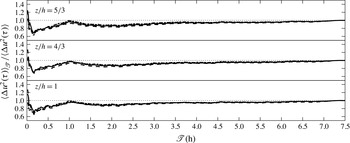
The convergence of statistics obtained from field data is evaluated by investigating the variability caused by changing the length of the averaging time interval ( $\mathscr{T}$ ) used for analysis (as done by Liu, Meneveau & Katz Reference Liu, Meneveau and Katz1994). Figure 1 shows that the second-order structure functions at $z/h=1$ , $4/3$ and $5/3$ converge within an averaging time interval of 3 h or less for the range of time lags of interest in the present analysis.

Figure 1.

The second-order streamwise temporal structure function ( $\langle {\rm\Delta}u({\it\tau})\rangle$ ) evaluated using an averaging time interval $\mathscr{T}$ normalized by the values calculated using the entire $7.5$ -h period of approximately stationary turbulence (no subscript). Results shown for time lags ${\it\tau}/(\ell _{{\it\epsilon}}/\langle u\rangle )=1$ , $5$ and $10$ (represented using dashed, solid and dash-dotted lines, respectively) at $z/h=1$ , $4/3$ and $5/3$ .

3.2 LES model set-up and analysis of results

The LES model employed here was described in detail by Pan, Chamecki & Isard (Reference Pan, Chamecki and Isard2014a ), Pan et al. (Reference Pan, Follett, Chamecki and Nepf2014b ). The effect of the model vegetation canopy on the flow is represented by a distributed drag that dissipates the kinetic energy of the flow,

where $C_{D}$ is the drag coefficient, $a$ is the leaf area density and $\tilde{\boldsymbol{u}}$ is the resolved velocity. The model maize canopy is homogeneous and infinite in both horizontal directions and the profile of leaf area density is obtained from experimental data (see Gleicher et al. Reference Gleicher, Chamecki, Isard, Pan and Katul2014, and reference therein). The effect of reconfiguration (i.e. bending and streamlining) of flexible canopy elements is represented using a drag coefficient modelled as a power-law function of velocity capped by an upper limit (Pan et al. Reference Pan, Follett, Chamecki and Nepf2014b ), $C_{D}=\text{min}((|\tilde{\boldsymbol{u}}|/A)^{B},C_{D,max})$ , where $A=0.22~\text{m}~\text{s}^{-1}$ , $B=-2/3$ and $C_{D,max}=0.8$ . When the velocity is low, the reconfiguration is negligible, and thus $C_{D}\approx C_{D,max}$ . When the velocity is high, the reconfiguration is strong, and thus $C_{D}\approx (|\tilde{\boldsymbol{u}}|/A)^{B}$ . The power-law exponent, $B=-2/3$ , is the Vogel number reported by theoretical and laboratory studies for simple bending (Alben, Shelley & Zhang Reference Alben, Shelley and Zhang2002; Gosselin, de Langre & Machado-Almeida Reference Gosselin, de Langre and Machado-Almeida2010).

Three LES runs using different grid resolution were conducted with a friction velocity, $u_{\star }=\langle u^{\prime }w^{\prime }\rangle _{h}^{1/2}=0.51~\text{m}~\text{s}^{-1}$ , where $u^{\prime }=u-\langle u\rangle$ and $w^{\prime }=w-\langle w\rangle$ are the turbulent fluctuations of streamwise and vertical velocity components and the subscript ‘ $h$ ’ indicates values at the top of the canopy ( $h=2.1$ m). The simulation domain was a box with $L_{x}\times L_{y}\times L_{z}=100h\times 40h\times 25h$ . The model canopy occupies the entire horizontal domain and the lowest one canopy height of the vertical domain. Table 1 shows the number of grid points, grid spacing and the number of vertical grids occupied by the model canopy used for fine, median and coarse resolution simulations. An additional median resolution simulation varying the friction velocity by a factor of $5$ ( $u_{\star }=0.1~\text{m}~\text{s}^{-1}$ ) was conducted to investigate the sensitivity of results to Reynolds number. Supplementary simulations on a smaller domain size ( $L_{x}\times L_{y}\times L_{z}=20h\times 20h\times 10h$ ) were conducted to determine the range of scales for which the spatial structure functions are not affected by domain size.

Table 1.

The number of grid points, grid spacing and the number of vertical grid points occupied by the model canopy used for fine, median and coarse resolution simulations.

The LES runs used the Lagrangian scale-dependent dynamic Smagorinsky subgrid-scale (SGS) model (Bou-Zeid, Meneveau & Parlange Reference Bou-Zeid, Meneveau and Parlange2005). The simulation was driven by a mean pressure gradient force. Viscous, Coriolis and buoyancy effects were not considered. Predictions of turbulence statistics up to the third order, the strength of quadrant events (e.g. sweeps, ejections and inward and outward interactions) and the fractions of momentum flux transported in different event quadrants agree well with the field experimental data (Pan et al. Reference Pan, Follett, Chamecki and Nepf2014b ). The median and coarse resolution simulations were conducted using a time step of ${\it\Delta}_{t}=0.005~\text{s}$ , while the fine resolution simulation were conducted using a time step of ${\it\Delta}_{t}=0.004~\text{s}$ . Turbulence statistics were calculated using statistically steady state flow periods of 45 min for the median and coarse resolution simulations and 30 min for the fine resolution simulation. For a given vertical position, statistics were calculated using the instantaneous velocity field within the entire horizontal domain at each time step and then averaged in time. The spatial structure functions were calculated using snapshots of the instantaneous velocity fields within the entire domain output every $1000$ time steps. For the median and coarse resolution simulations, $540$ snapshots were output every $5~\text{s}$ . For the fine resolution simulation, $450$ snapshots were output every $4~\text{s}$ . The temporal structure functions were calculated using time series output every time step at a specified cross-flow sectional plane.

In the analysis of simulation results, the displacement height was determined as the mean height of the distributed drag following Thom (Reference Thom1971) and Jackson (Reference Jackson1981), yielding $d_{0}/h=0.78$ . The dissipation rate of TKE was estimated from the SGS dissipation rate (Bou-Zeid et al. Reference Bou-Zeid, Higgins, Huwald, Meneveau and Parlange2010), which is given by

where ${\bf\tau}_{SGS}$ is the SGS stress tensor and $\tilde{\unicode[STIX]{x1D64E}}=(\boldsymbol{{\rm\nabla}}\tilde{\boldsymbol{u}}+(\boldsymbol{{\rm\nabla}}\tilde{\boldsymbol{u}})^{\text{T}})/2$ is the filtered strain rate tensor. The scale-dependent SGS model provides reliable estimates of the cascade of TKE from resolved scales to subgrid scales (Bou-Zeid et al. Reference Bou-Zeid, Meneveau and Parlange2005). The convergence of LES results is also evaluated by investigating the change in the turbulence statistics with the length of the averaging time interval ( $\mathscr{T}$ ) used for analysis. 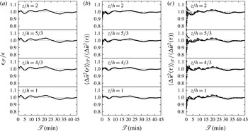For the median resolution simulation with $u_{\star }=0.51~\text{m}~\text{s}^{-1}$ , figure 2 shows that results of the TKE dissipation rate and the second-order structure functions at $1<z/h<2$ converge within an averaging time interval of 10 min or less. Simulations with alternative grid resolution and friction velocity require a similar averaging time interval for these statistics to converge (not shown). The use of spatial averaging for the analysis of LES results yields shorter averaging periods required for convergence in comparison to those needed for the field data.

Figure 2.

The results of the TKE dissipation rate ( ${\it\epsilon}$ ), the second-order streamwise spatial structure function ( $\langle {\rm\Delta}\tilde{u} ^{2}(r)\rangle$ ) and the second-order streamwise temporal structure function ( $\langle {\rm\Delta}\tilde{u} ^{2}({\it\tau})\rangle$ ) evaluated using an averaging time interval $\mathscr{T}$ normalized by the values calculated using the entire statistically steady state periods (no subscript). Results are obtained from the median resolution simulation with $u_{\star }=0.51~\text{m}^{-1}$ and shown for selected heights, $z/h=1$ , $4/3$ , $5/3$ and $2$ . The structure functions are shown for selected scales, $r/\ell _{{\it\epsilon}}=1$ , $5$ and $10$ (b) and ${\it\tau}/(\ell _{{\it\epsilon}}/\langle u\rangle )=1$ , $5$ and $10$ (c), represented by dashed, solid and dash-dotted lines, respectively.

4.1 Characteristics of the roughness sublayer above the model canopy

The region of interest here is the shear layer above the model canopy and within the lowest $20\,\%$ of the domain, corresponding to the region $1<z/h<5$ . Within this region, simulations with $u_{\star }=0.51~\text{m}~\text{s}^{-1}$ yield the Reynolds number for the flow, $\mathit{Re}=\ell _{{\it\epsilon}}u_{\star }/{\it\nu}$ , ranging from $2.6\times 10^{4}$ to $1.4\times 10^{5}$ . The roughness Reynolds number, $\mathit{Re}^{\star }=hu_{\star }/{\it\nu}=7.2\times 10^{4}$ , where $h=2.1$ m is the canopy height. The Taylor microscale Reynolds number, $\mathit{Re}_{{\it\lambda}}={\it\lambda}u_{\star }/{\it\nu}$ , ranges from $1.1\times 10^{3}$ to $2.8\times 10^{3}$ . For the median resolution simulation, the effective Reynolds number, $\mathit{Re}_{LES}=({\it\eta}/{\it\eta}_{LES})^{4/3}Re$ (Muschinski Reference Muschinski1996), ranges from $34$ to $236$ . The effective roughness Reynolds number, $\mathit{Re}_{LES}^{\star }=({\it\eta}/{\it\eta}_{LES})^{4/3}\mathit{Re}^{\star }=92$ . Here ${\it\nu}=1.48\times 10^{-5}$ m $^{2}$ s $^{-1}$ is the kinematic viscosity of air, 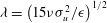${\it\lambda}=\left(15{\it\nu}{\it\sigma}_{u}^{2}/{\it\epsilon}\right)^{1/2}$ is the Taylor microscale, ${\it\eta}=\left({\it\nu}^{3}/{\it\epsilon}\right)^{1/4}$ is the Kolmogorov length scale, ${\it\eta}_{LES}=c_{s}{\it\Delta}$ is the SGS mixing length, $c_{s}$ is the Smagorinsky coefficient and ${\it\Delta}=({\it\Delta}_{x}{\it\Delta}_{y}{\it\Delta}_{z})^{1/3}$ is the characteristic grid spacing (Scotti, Meneveau & Lilly Reference Scotti, Meneveau and Lilly1993). The roughness Reynolds number varies with friction velocity but not with grid resolution. The effective roughness Reynolds number varies with grid resolution but not with friction velocity. The fine and coarse resolution simulations yield $\mathit{Re}_{LES}^{\star }=136$ and $54$ , respectively.

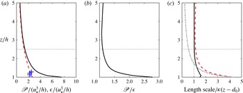
Figure 3(a) shows the vertical profiles of the production and dissipation rates of TKE normalized by $u_{\star }^{3}/h$ . These dimensionless vertical profiles are independent of grid resolution and friction velocity (not shown). The insensitivity of ${\it\epsilon}$ estimated using (3.3) to grid spacing implies that the rate of energy cascade provides reasonable estimates of the rate of TKE dissipation. The reliability of LES estimates of ${\it\epsilon}/(u_{\star }^{3}/h)$ immediately above the model canopy is further supported by the good agreement with dissipation rates estimated from PIV measurements above a mature maize canopy obtained by van Hout et al. (Reference van Hout, Zhu, Luznik, Katz, Kleissl and Parlange2007) (dashed line compared with crosses in figure 3 a). Close to the canopy top, the ratio $\mathscr{P}/{\it\epsilon}\approx 3$ (figure 3 b), a value much greater than that observed in the inertial layer of wall turbulence and more characteristic of mixing layers (Rogers & Moser Reference Rogers and Moser1994). For $z/h>2.5$ , the production and dissipation of TKE are almost in balance (figure 3 a,b) and the production length scale ( $\ell _{\mathscr{P}}=u_{\star }^{3}/\mathscr{P}$ ) approaches ${\it\kappa}(z-d_{0})$ (solid line compared with vertical dotted line in figure 3 c). These features indicate the recovery of an inertial layer, and thus $z/h=2.5$ is determined as the upper boundary of the canopy roughness sublayer.

Figure 3.

LES results of the production ( $\mathscr{P}$ ) and dissipation ( ${\it\epsilon}$ ) rates of TKE normalized by $u_{\star }^{3}/h$ (a), the ratio $\mathscr{P}/{\it\epsilon}$ (b) and the length scales ( $\ell _{\mathscr{P}}$ , $\ell _{{\it\epsilon}}$ and $\ell _{s}$ ) normalized by ${\it\kappa}(z-d_{0})$ (c) against vertical distance from the ground ( $z$ ) normalized by canopy height ( $h$ ). In (a), solid and dashed lines indicate $\mathscr{P}/(u_{\star }^{3}/h)$ and ${\it\epsilon}/(u_{\star }^{3}/h)$ , respectively. Crosses indicate estimates of ${\it\epsilon}/(u_{\star }^{3}/h)$ from PIV measurements above a maize canopy (van Hout et al. Reference van Hout, Zhu, Luznik, Katz, Kleissl and Parlange2007). In (c), solid, dashed and dash-dotted lines indicate $\ell _{\mathscr{P}}/{\it\kappa}(z-d_{0})$ , $\ell _{{\it\epsilon}}/{\it\kappa}(z-d_{0})$ and $\ell _{s}/{\it\kappa}(z-d_{0})$ , respectively. Here $u_{\star }$ is the friction velocity, $d_{0}$ is the displacement height and $(z-d_{0})$ , $\ell _{s}$ , $\ell _{\mathscr{P}}$ , and $\ell _{{\it\epsilon}}$ are the inertial layer, mixing layer, production and dissipation length scales, respectively. The horizontal dotted lines indicate the upper boundary of the canopy roughness layer, $z/h=2.5$ .

Within the roughness sublayer above the canopy ( $1<z/h<2.5$ ), two external length scales coexist: $(z-d_{0})$ associated with inertial layer eddies and $\ell _{s}=\langle u\rangle _{z=h}/(\partial \langle u\rangle /\partial z)_{z=h}$ associated with mixing-layer eddies (Raupach et al. Reference Raupach, Finnigan and Brunet1996). As expected, $\ell _{s}$ (dash-dotted line in figure 3 c) is much larger than ${\it\kappa}(z-d_{0})$ near the canopy top, and it becomes significantly smaller than ${\it\kappa}(z-d_{0})$ above the canopy roughness sublayer ( $z/h>2.5$ ). Even though the production length scale (solid line in figure 3 c) increases as the canopy top is approached, it does not reflect the large coherence of mixing-layer eddies that scale on $\ell _{s}$ . Interestingly, the dissipation length scale $\ell _{{\it\epsilon}}$ (dashed line in figure 3 c) provides a smooth transition from $\ell _{s}$ near the canopy top to ${\it\kappa}(z-d_{0})$ above the canopy roughness sublayer. These LES results suggest that $\ell _{{\it\epsilon}}$ has the potential to characterize the transition from a mixing-layer flow close to the canopy top to a boundary-layer flow above the canopy roughness sublayer. Thus, LES results support the theoretical analysis in § 2 that $\ell _{{\it\epsilon}}$ characterizes the shear-production range turbulent motions.

4.2 Evaluation of the second-order streamwise temporal structure function

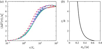
We start by using results of temporal and spatial structure functions from the median resolution simulation with $u_{\star }=0.51~\text{m}~\text{s}^{-1}$ to assess the validity of Taylor’s hypothesis of frozen turbulence in the canopy shear layer. Figure 4(a) shows that the temporal structure functions converted using Taylor’s hypothesis ( $\langle {\rm\Delta}\tilde{u} ^{2}(r={\it\tau}\langle u\rangle )\rangle$ ) agree well with the spatial structure functions ( $\langle {\rm\Delta}\tilde{u} ^{2}(r)\rangle$ ) at small scales, but asymptote faster to the maximum value ( $2\langle {u^{\prime }}^{2}\rangle$ ). The cutoff scale for the validity of Taylor’s hypothesis increases with increasing distance from the canopy top. Specifically for $z/h>4/3$ (blue, cyan, black, green and grey dashed and solid lines in figure 4 a), the cutoff scale is greater than $r/\ell _{{\it\epsilon}}=3$ . The inapplicability of Taylor’s hypothesis is expected, given the large values of turbulence intensity ( ${\it\sigma}_{u}/\langle u\rangle$ ) typically observed in canopy shear layers (figure 4 b). Note that spatial structure functions collapse using the $\ell _{{\it\epsilon}}$ -scaling, but their temporal counterparts do not due to inapplicability of Taylor’s hypothesis for the production and inactive ranges. Results from simulation using different grid resolutions or friction velocity yield the same conclusion (not shown). The non-equivalence between spatial and temporal structure functions exposes the limitations of field experimental data in assessing structure function scalings (and other related statistics such as correlation functions, integral length scales, etc.) in canopy shear layers.

Figure 4.

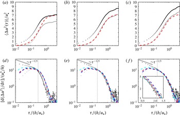
(a) LES results of second-order streamwise spatial structure functions ( $\langle {\rm\Delta}\tilde{u} ^{2}(r)\rangle$ ; solid lines) and temporal structure functions converted using Taylor’s hypothesis ( $\langle {\rm\Delta}\tilde{u} ^{2}(r={\it\tau}\langle u\rangle )\rangle$ ; dashed lines) normalized by the square of friction velocity ( $u_{\star }^{2}$ ) against spatial separation ( $r$ ) normalized by the dissipation length scale ( $\ell _{{\it\epsilon}}$ ). Red, magenta, blue, cyan, black, green and grey lines indicate results for $1<z/h<2$ with an increment of ${\rm\Delta}z/h=1/6$ . (b) The turbulence intensity ( ${\it\sigma}_{u}/\langle u\rangle$ ) against vertical distance from the ground ( $z$ ) normalized by canopy height ( $h$ ), where ${\it\sigma}_{u}$ and $\langle u\rangle$ are the standard deviation and the mean of the streamwise velocity, respectively.

Figure 5 shows evaluation of LES results of the second-order temporal structure functions against field experimental data. Note that both hot-film and PIV measurements within the roughness sublayer above maize canopies confirmed the $-5/3$ scaling in the inertial subrange of the spectrum of the streamwise velocity (Shaw et al. Reference Shaw, Silversides and Thurtell1974; Wilson et al. Reference Wilson, Ward, Thurtell and Kidd1982; van Hout et al. Reference van Hout, Zhu, Luznik, Katz, Kleissl and Parlange2007). Within the inertial subrange, Taylor’s hypothesis of frozen turbulence is valid (see figure 4), and therefore the second-order streamwise temporal structure function ( $\langle {\rm\Delta}u^{2}({\it\tau})\rangle$ ) and the energy density ( $\text{d}\langle {\rm\Delta}u^{2}({\it\tau})\rangle /\text{d}{\it\tau}$ ) are expected to scale as ${\it\tau}^{2/3}$ and ${\it\tau}^{-1/3}$ , respectively. Due to non-negligible path averaging errors associated with sonic anemometer measurements at the frequencies that correspond to the inertial subrange (Horst & Oncley Reference Horst and Oncley2006), the raw field data of $\text{d}\langle {\rm\Delta}u^{2}({\it\tau})\rangle /\text{d}{\it\tau}$ at small scales do not follow ${\it\tau}^{-1/3}$ exactly (black dots compared with grey solid lines in figure 5 d–f). Nevertheless, the ${\it\tau}^{-1/3}$ dependence of $\text{d}\langle {\rm\Delta}u^{2}({\it\tau})\rangle /\text{d}{\it\tau}$ in the inertial subrange is approached by raw data from sonic anemometer measurements.

Figure 5.

Evaluation of LES results of the normalized second-order temporal structure function ( $\langle {\rm\Delta}\tilde{u} ^{2}({\it\tau})\rangle /u_{\star }^{2}$ ; a–c) and the energy density ( $[\text{d}\langle {\rm\Delta}u^{2}({\it\tau})\rangle /\text{d}{\it\tau}]/(u_{\star }^{3}/h)$ ; d–f) against field experimental data for $z/h=1$ (a,d), $4/3$ (b,e) and $5/3$ (c,f). Blue, red and cyan dashed lines indicate LES results from coarse, median and fine resolution simulations, while black and grey dots indicate the structure function of raw and filtered experimental velocity data. The vertical dotted lines in (d–f) indicate the cutoff scales for the median resolution simulation, ${\it\tau}=4{\it\Delta}_{x}/\langle u\rangle$ , where ${\it\Delta}_{x}=0.5~\text{m}$ . The filter size applied to experimental velocity data, ${\it\Delta}_{{\it\tau}}=(4/\sqrt{2}){\it\Delta}_{x}/\langle u\rangle$ , are 0.87, 0.61 and 0.51 s for $z/h=1$ , $4/3$ and $5/3$ , respectively.

Because LES does not resolve SGS motions, the structure function of the resolved velocity ( $\tilde{u}$ ) is expected to be smaller than the raw field data (dashed lines compared with black dots in figure 5 a–c). The vertical dotted lines in figure 5(d–f) indicate the cutoff scales for the median resolution simulation, sitting at the transition from the inertial subrange to the overlap of the shear-production and inactive ranges. At subgrid scales, reducing the grid spacing improves the capability of reproducing the energy density (cyan dashed lines compared with red dashed lines in figure 5 d–f to the left of the vertical dotted lines). At resolved scales, the fine and median resolution simulations yield the same energy density, whereas the coarse resolution simulation exhibits a pile up of energy (blue dashed lines compared with cyan and red dashed lines in the inset in figure 5 f). In addition, for the fine and median resolution simulations, the scale-dependent dynamic SGS model predicts the same profile of the Smagorinsky coefficient, whereas the coarse resolution simulation results show a reduction of the Smagorinsky coefficient (not shown). Both the pile up of energy at resolved scales and the reduction of the Smagorinsky coefficient indicate insufficient resolution for the coarse resolution simulation (Bou-Zeid et al. Reference Bou-Zeid, Meneveau and Parlange2005). Thus, we conclude that the median grid resolution used here corresponds to the minimum resolution required for the adequate reproduction of turbulence above the maize canopy studied here. For $z/h=1$ , LES results slightly overestimated the energy density of raw experimental data at resolved scales (dashed lines compared with black dots to the right of the vertical dotted line in figure 5 d). For $z/h=4/3$ and $5/3$ , LES results reproduced the energy density of raw experimental data at resolved scales (dashed lines compared with black dots to the right of the vertical dotted lines in figure 5 e,f).

To provide a better basis for comparison with LES, a Gaussian filter (Pope Reference Pope2000) is applied to the experimental data. The filter size, ${\it\Delta}_{{\it\tau}}=(4/\sqrt{2}){\it\Delta}_{x}/\langle u\rangle$ , is chosen to maintain turbulent motions at spatial scales greater than $4{\it\Delta}_{x}$ (i.e. the scales resolved in the LES). LES results reproduced the second-order streamwise temporal structure function of filtered experimental velocity data for $z/h=4/3$ and $5/3$ (red dashed lines compared with grey dots in figure 5 b,c). Close to the canopy top, the removal of energy from large scales is enhanced by wake production behind individual canopy elements, a feature not represented in the LES model. As expected, for $z/h=1$ , the LES results overestimated the structure function of filtered experimental velocity data, especially at large scales ${\it\tau}/(h/u_{\star })>0.5$ (red dashed line compared with grey dots in figure 5 a). Results presented in figure 5 suggest that the fine and median resolution simulations are capable of reproducing details of second-order structure functions above the canopy for scales larger than those in the inertial subrange (a finer grid resolution would be needed for inertial subrange scales to be reliable). The analysis presented next focuses on the overlap of shear-production and inactive ranges, where motions are well resolved in the simulations.

Figure 6.

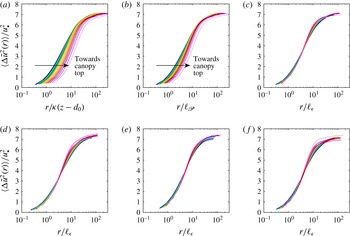
LES results of the normalized second-order streamwise spatial structure function of ( $\langle {\rm\Delta}\tilde{u} ^{2}(r)\rangle /u_{\star }^{2}$ ) against streamwise spatial separation ( $r$ ) normalized by ${\it\kappa}(z-d_{0})$ (a), $\ell _{\mathscr{P}}$ (b) and $\ell _{{\it\epsilon}}$ (c–f). Here $(z-d_{0})$ , $\ell _{\mathscr{P}}$ and $\ell _{{\it\epsilon}}$ are the inertial layer, production and dissipation length scales. Solid lines of different colours indicate results at different heights within the shear layer above the canopy ( $1<z/h<2.5$ ), with an increment of ${\rm\Delta}z/h=1/8$ , $1/12$ and $1/16$ for coarse (e), median (a–c,f) and fine (d) resolution simulations. Arrows indicate decreasing vertical coordinate towards the canopy top. Simulations were conducted with $u_{\star }=0.51~\text{m}~\text{s}^{-1}$ (a–e) and $0.1~\text{m}~\text{s}^{-1}$ (f).

4.3 Scaling of the second-order streamwise spatial structure function

Figure 6(a–c) shows results of the second-order streamwise spatial structure function of resolved velocity ( $\langle {\rm\Delta}\tilde{u} ^{2}(r)\rangle$ ) from the median resolution simulation with $u_{\star }=0.51~\text{m}~\text{s}^{-1}$ against the eddy size ( $r$ ) normalized by three different length scales ( ${\it\kappa}(z-d_{0})$ , $\ell _{\mathscr{P}}$ and $\ell _{{\it\epsilon}}$ ). Within the roughness sublayer layer above the canopy ( $1<z/h<2.5$ ), the inertial layer, production and dissipation length scales ( $(z-d_{0})$ , $\ell _{\mathscr{P}}$ and $\ell _{{\it\epsilon}}$ ) are not proportional to each other (figure 3 b). LES runs with varying domain sizes (not shown) suggest that the current domain provides reliable estimates of $\langle {\rm\Delta}\tilde{u} ^{2}(r)\rangle$ for $r/\ell _{{\it\epsilon}}<20$ . Curves representing $\langle {\rm\Delta}\tilde{u} ^{2}(r)\rangle /u_{\star }^{2}$ at different heights do not collapse when $r$ is normalized by ${\it\kappa}(z-d_{0})$ (figure 6 a) or $\ell _{\mathscr{P}}$ (figure 6 b), but do collapse when $r$ is normalized by $\ell _{{\it\epsilon}}$ (figure 6 c). The collapse against $\ell _{{\it\epsilon}}$ is robust to changes in grid resolution and friction velocity (figure 6 d–f). These results indicate that $\ell _{{\it\epsilon}}$ rather than $(z-d_{0})$ or $\ell _{\mathscr{P}}$ is the correct scaling for the second-order structure function within the shear layer above the canopy.

Figure 7.

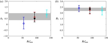
Ranges of parameters $A_{2}$ (a) and $B_{2}$ (b) in (2.10) estimated for each simulation by applying a least square fitting to the logarithmic region ( $\text{max}(\ell _{{\it\epsilon}},4{\it\Delta}_{x})<r<0.2L_{z}$ ) of individual curves in figure 6(c–f) against the effective roughness Reynolds number ( $\mathit{Re}_{LES}^{\star }$ ). Blue, red and cyan error bars indicate the ranges estimated for coarse, median and fine resolution simulation with $u_{\star }=0.51~\text{m}~\text{s}^{-1}$ , while the black error bar indicates the ranges estimated for median resolution simulation with $u_{\star }=0.1~\text{m}~\text{s}^{-1}$ . Circles that are the same colour as error bars indicate an additional set of parameters $A_{2}$ and $B_{2}$ estimated for each simulation by applying a least square fitting to the logarithmic region of all curves in figure 6(c–f). Open and filled circles represent simulations with $u_{\star }=0.51$ and $0.1~\text{m}~\text{s}^{-1}$ , respectively. Grey areas in (a) and (b) indicate the ranges $0.37<A_{2}<0.97$ and $2.16<B_{2}<2.44$ estimated by de Silva et al. (Reference de Silva, Marusic, Woodcock and Meneveau2015) using laboratory and field experimental data obtained in the inertial layer of wall turbulence.

The overlap of the shear-production and inactive ranges corresponds to spatial scales greater than the integral length scale ( $r>\ell \propto \ell _{{\it\epsilon}}$ ) and much smaller than the boundary-layer thickness ( $r\ll {\it\delta}\sim L_{z}$ ). In addition, results in § 4.2 suggest that LES resolves spatial scales greater than $4{\it\Delta}_{x}$ . Thus we estimate that the resolved overlap of the shear-production and inactive ranges for the present simulation consists of spatial scales $\text{max}(\ell _{{\it\epsilon}},4{\it\Delta}_{x})<r<0.2L_{z}$ . This range of spatial scales roughly corresponds to $1<r/\ell _{{\it\epsilon}}<10$ , where a $\ln (r/\ell _{{\it\epsilon}})$ law is observed for LES results of the second-order structure function (figure 6 c–f). Figure 7 shows the ranges of parameters $A_{2}$ and $B_{2}$ in (2.10) estimated for each simulation by applying a least square fitting to the logarithmic region ( $\text{max}(\ell _{{\it\epsilon}},4{\it\Delta}_{x})<r<0.2L_{z}$ ) of individual curves in figure 6(c–f). An additional set of parameters $A_{2}$ and $B_{2}$ is estimated for each simulation by applying a least square fitting to all the heights together (circles in figure 7). The ranges of $A_{2}$ and $B_{2}$ estimated for fine and median resolution simulations (cyan, red and black error bars in figure 7) are in reasonable agreement with those estimated by de Silva et al. (Reference de Silva, Marusic, Woodcock and Meneveau2015) using laboratory and field experimental data obtained in the inertial layer of wall turbulence ( $0.37<A_{2}<0.97$ and $2.16<B_{2}<2.44$ , represented by grey areas in figure 7). Varying $u_{\star }$ by a factor of $5$ can change the displacement height by $10\,\%$ (Pan, Chamecki & Nepf Reference Pan, Chamecki and Nepf2016), but it induces negligible changes in the estimated ranges for $A_{2}$ and $B_{2}$ (black error bar compared with red error bar in figure 7). Figure 6(c–f) confirms the validity of the dimensional analysis presented in § 2 in the shear layer above a canopy, while figure 7 suggests the possibility of the existence of a fairly universal set of parameters $A_{2}$ and $B_{2}$ that may hold for a wide range of shear flows.