1 Introduction
The automatic acquisition of lexical information from text corpora is of great importance especially for parsing and lexicography. Many parsers rely on valence information in the lexicon in order to eliminate erroneous parses. Many dictionaries nowadays contain syntactic information for their entries, and contemporary grammatical formalisms (e.g. head-driven phrase structure grammar) are based on the richness in linguistic information at the lexicon level.
Detecting the complements of a verb is an interesting application of lexical acquisition. Verb complements are the sentence constituents that are selected for by the verb. Among the dependents of a verb (children nodes of a verb in the syntactic tree of the sentence, i.e. complements and adjuncts), complements are key participants in the event described by the verb, while adjuncts comprise secondary information concerning the ‘setting’ of the event (its context, location etc.). In the following two examples it is clear that Anne is a complement of the verb σχετíζoμαi (to be involved) in the first sentence, and an adjunct of the verb τpωω (to eat) in the second.

In this paper we address the issue of learning verb complements in Modern Greek texts using machine learning techniques. As a treebank and wide coverage parsers for Modern Greek are not available, we make use of input that is automatically annotated only up to the phrase level, where the verb dependents are not identified. Using minimum resources for preprocessing enables the present methodology to be applied to languages that are not extensively equipped with linguistic resources. On the other hand, low-level preprocessing leads to non-dependents appearing among the candidate complements and adjuncts, and constituting a major source of noise. As a result, the number of complements (positive examples) among the candidates is significantly smaller than that of the noisy candidates (negative examples). This disproportion causes a significant drop in accuracy when predicting the minority class (complements).
Previous approaches to identifying complements use higher-level resources for preprocessing (treebanks or parsers) and receive as input the dependents of the verb (complements and adjuncts) and then distinguish between the two. In this work we distinguish complements directly from all the remaining sentence terms, and adjuncts are not identified. The reason is that, as a future direction, the outcome of the present work is to be incorporated into the process of automatically acquiring verb subcategorization information for Modern Greek, where adjunct information is not useful.
The disproportion between the two classes causes a significant drop in the accuracy when predicting the minority class (complements). To overcome this problem we apply one-sided sampling and Tomek (Reference Tomek1976) links to the training data to obtain a more balanced subset of the initial training set by pruning out noisy and redundant instances of the majority class. This sampling approach has been used in the past in several domains such as image processing and medicine, and we apply it here for the first time to lexical acquisition. A novel variation proposed in the present paper for detecting Tomek links is the distance metric used to determine the examples that are safe to remove. Due to the fact that features in the training vectors take exclusively nominal values, we experiment with the value difference metric (Stanfill and Waltz Reference Stanfill and Waltz1986) apart from the Euclidean distance, traditionally used in one-sided sampling. The former, by taking into account the correlation of a nominal value with the output class, is more suitable for this type of features. This claim is supported by Stanfill and Waltz (Reference Stanfill and Waltz1986), and also by the experimental results of this work. It should be noted that the resulting subset is more balanced than the initial one, but still does not consist of an exactly equal number of examples of the two classes. We will, however, refer to it as the balanced subset.
A set of broadly used learners (decision trees, IB1 and its weighted variation, Naïve Bayes, Bayesian networks) is then trained with the reduced training data and used to classify new instances. The learners were chosen to cover a wide range of learning techniques (instance-based learning, tree-based learning, Bayesian learning) with the aim to compare their performance on the same dataset for the specific linguistic task.
2 Modern Greek
In this section we describe the properties of Modern Greek that are closely related to this application. Concerning morphology, Modern Greek is highly inflectional. For distinguishing complements, a key morphological feature of nouns, adjectives and pronouns is their case (nominative, genitive or accusative). Key features for verbs are their voice (active or passive), and certain semantic attributes: whether a verb is copular or not, personal or impersonal, as well as the verb's mode. Mode is the verb property that determines the semantic relation between the verb and its subject. The subject may a. affect (active mode), b. be affected by (passive mode), c. affect and be affected by (middle mode), d. neither affect nor be affected by (neutral mode) the action denoted by the verb.
Concerning sentence structure, Modern Greek is a ‘semi free word order’ language. Unlike English, phrases (noun, verb, prepositional or adverbial) can form a grammatically correct sentence in almost any permutation. More specifically, the arguments of a verb do not have fixed positions with respect to the verb and are therefore determined primarily by their morphology rather than their position.
It should be made clear that by complement we mean every syntactic argument of the verb except for the subject. From a syntax point of view a complement may be a noun phrase in the accusative case (direct object), or in the genitive case (indirect object), a prepositional phrase (prepositional object), a secondary clause (Klairis and Babiniotis Reference Klairis and Babiniotis1999). Very often the complements appear within the verb phrase itself in the form of weak personal pronouns. The predicative (usually a noun phrase in the nominative) of a copular verb (a verb assigning an attribute to a subject) is also a complement.
Very often noun phrases in the accusative case (underlined in the following examples) play adverbial roles (usually denoting time) and are not complements of the verb in the sentence. Certain prepositions also can introduce adverbial prepositional phrases except for complements.
The following two examples (a and b) are the same sentence, that is syntactically ambiguous. Nominals in the genitive, like the definite noun τ oεΓíαn n(John's) in example (a) often denote possession (though they seldom appear in a separate phrase – they normally form one noun phrase with the possessed entity) and are not frames of the verb in the sentence. In sentence (a) the verb δínω (to give), which normally takes two complements (the ‘givee’ and the ‘given’), appears only with one (τoβiβλíoτoεΓíαn n– John's book) and the second is missing, according to the bracketing. In example (b) it appears with both its complements. Here τoβiβ λío(the book-accusative NP) and τoεΓíαn n(John's-genitive NP) are the direct and the indirect object respectively. Resolution of such ambiguities depends on correct preprocessing (in this case phrase boundary detection). VP and NP stand for verb and noun phrase respectively.
From the above examples it is clear that the morphological features described previously are not sufficient on their own for the detection of complements. These particular ambiguities are very hard to resolve without the use of higher-level semantic information. When linguistic information regarding the candidate complement is taken into account as well as information regarding the context of the candidate complement, however, many cases of ambiguity can be correctly resolved, as is shown in section 8.3.
3 Previous work
Previous work focusing specifically on the automatic complement-adjunct distinction varies from generating candidate complements and utilizing statistical filtering on the candidates in order to filter out adjuncts (Aldezabal, Aranzabe, Atutxa, Gojenola and Sarasola 2002) to making use of memory-based learning methods (Buchholz Reference Buchholz1998) and decision trees (Merlo and Leybold Reference Merlo and Leybold2001).
Buchholz (Reference Buchholz1998) describes a set of experiments performed on the part-of-speech tagged and phrase structured part of the Wall Street journal. Every verb phrase along with its complement and adjunct siblings is encoded into a feature-value vector, where relevant linguistic properties (syntactic categories and function tags) as well as subcategorization information constitute a data instance used for memory-based learning of previously unseen instances. The last feature of the vector corresponds to the target class. Buchholz reports a generalization accuracy of 91.6%.
Aldezabal et al. (Reference Aldezabal, Aranzabe, Atutxa, Gojenola and Sarasola2002) work on Basque. They apply mutual information and Fisher's exact test to verb-case pairs (a case is any type of argument) which were obtained from a partially parsed newspaper corpus of 1.3 million words. Evaluation was performed against human tagging of the dependents of ten test verbs inside (reaching an f-measure of 95%) and outside (reaching an f-measure of 55%) the context of the sentence.
Merlo and Leybold (Reference Merlo and Leybold2001) use decision trees to distinguish prepositional arguments from prepositional modifiers. They use lexical head, semantic verb class, preposition and noun cluster information as well as conditional probabilities of prepositional phrases given verbal lexical heads in order to form their instance vector. Their training set consists of 3,692 and their test set of 400 instances. They report an accuracy of 86.5%.
Previous work on the automatic acquisition of verb subcategorization information has focused mainly on statistical filtering methods applied to generated putative subcategorization frames. Subcategorization frames are combinations of complements. Most of these approaches distinguish complements from adjuncts as a first step in order to avoid the sparse data problem. Sarkar and Zeman (Reference Sarkar and Zeman2000), for instance, iteratively reduce the size of the candidate frame in order to filter out adjuncts. Briscoe and Carroll (Reference Briscoe and Carroll1997) as well as Korhonen, Gorrell and McCarthy (2000) use the same, more sophisticated grammar and parsing tool for argument/adjunct distinction. Ersan and Charniak (Reference Ersan and Charniak1995) make use of a Probabilistic context-free grammar (PCFG) for the same purpose. Hypothesized frames are generated through methodologies varying in the extent of preprocessing of the corpus data used as input to the learning process, the number of frames learned, whether the set of frames is known beforehand or not. The filtering methods employed are: binomial hypothesis testing (Brent Reference Brent1993; Manning Reference Manning1993; Ersan and Charniak 1996; Briscoe and Carroll Reference Briscoe and Carroll1997; Korhonen et al. Reference Korhonen, Gorrell and McCarthy2000; Sarkar and Zeman Reference Sarkar and Zeman2000), the log likelihood ratio (Korhonen et al. Reference Korhonen, Gorrell and McCarthy2000; Sarkar and Zeman Reference Sarkar and Zeman2000), the t-test (Sarkar and Zeman Reference Sarkar and Zeman2000), maximum likelihood estimation of relative frequencies (Korhonen et al. Reference Korhonen, Gorrell and McCarthy2000).
Unlike previous approaches, in this paper, as mentioned earlier, verb complements are distinguished from all the remaining sentence constituents and not just from adjuncts. Adjunct information is not important as adjuncts do not contribute to the acquisition of verb subcategorization information (information regarding the set of arguments that a verb selects for, i.e. subcategorization frames), which is the future application of the outcome of the present work. We start off by taking into account the linguistic properties described in the previous section, that play a significant role to complement identification (Klairis and Babiniotis Reference Klairis and Babiniotis1999; Karanikolas et al. Reference Karanikolas, Spyropoulos, Aggelidou, Betsopoulou, Grigoriadis, Kandros, Karpouza, Lanaris, Moumtzakis, Tombaidis and Tsolakis2004): the phrase type, part-of-speech information, the grammatical case, the verb voice and mood, copularity, context information. We adopt the feature vector structure of Buchholz (Reference Buchholz1998). Unlike Buchholz, we do not use subcategorization information or extensive function tags, because they are unavailable to us due to our lower-level preprocessing. All of the selected features are described in detail in section 5. Unlike Buchholz and most of the previous approaches, we do not have any information regarding the verb dependents (complements and adjuncts) and therefore use a window of phrases preceding and following the verb (capturing thereby the freedom in Modern Greek sentence structure, where complements may precede the verb) and treat these phrases as candidate complements. Apart from instance-based learning, used by Buchholz, we experiment with various other learners to learn complements. We then reduce the number of redundant and noisy training examples by applying a sampling method called one-sided sampling to improve the performance of the prediction of complement-class examples. The approach is described in detail in the following sections.
4 Data preprocessing
The corpus used in this work is a collection of the ILSP/ELEFTHEROTYPIA and ESPRIT 860 (300,000 words) and a 500,000 word part of the DELOS Modern Greek corpora. These corpora are treated together as one corpus, because their size is too small for them to be treated independently.
The ILSP/ELEFTHEROTYPIA (Hatzigeorgiu, Gavriilidou, Piperidis, Carayannis, Papakostopoulou, Spiliotopoulou, Vacalopoulou, Labropoulou, Mantzari, Papageorgiou and Demiros Reference Hatzigeorgiu, Gavriilidou, Piperidis, Carayannis, Papakostopoulou, Spiliotopoulou, Vacalopoulou, Labropoulou, Mantzari, Papageorgiou and Demiros2000) and ESPRIT 860 (Partners of ESPRIT-291/860 1986) corpora (a total of approximately 300,000 words) are balanced in genre and domain and manually annotated with complete morphological information. Further (phrase structure) information is obtained automatically as described in sections 4.1 and 4.2 below.
The DELOS Corpus (Kermanidis, Fakotakis and Kokkinakis Reference Kermanidis, Fakotakis and Kokkinakis2002) is a collection of economic domain texts of approximately five million words and of varying genre (press reportage, news, articles, interviews and scientific studies). It has been automatically annotated from the ground up. Morphological tagging of DELOS was performed by an analyzer for Modern Greek that is based on Koskenniemi's two-level morphology model and utilizes a lexicon of more than 60,000 lemmata (Sgarbas, Fakotakis and Kokkinakis Reference Sgarbas, Fakotakis and Kokkinakis2000). The provided information includes part-of-speech (pos) tagging for all words, case tagging for nouns, adjectives and pronouns, voice tagging for verbs, type tagging for pronouns (relative/interrogative etc.) and type tagging for conjunctions (coordinating/subordinating). Precision and recall values in pos tagging reach 84–88% and 95–98% respectively. Concerning morphological features that play a key role in this particular application, case tagging reaches an accuracy exceeding 94%, and voice tagging for verbs 84%. Phrase structure information is again obtained automatically as described in sections 4.1 and 4.2 below. DELOS also contains subject-verb-object information detected by a shallow parser based on a set of empirical rules and limited to detecting nominal and prepositional objects as opposed to entire clauses (Kermanidis et al. Reference Kermanidis, Fakotakis and Kokkinakis2002). The performance of the parser reaches 70% precision and recall when tested on 500 verb occurrences.
4.1 Chunking
All the corpora have been phrase-analyzed by the chunker described in detail in Stamatatos, Fakotakis and Kokkinakis (2000). Noun (NP), verb (VP), prepositional (PP), adverbial phrases (ADP) and conjunctions (CON) are detected via multi-pass parsing. The chunker is based on a small keyword lexicon containing some 450 keywords (articles, pronouns, etc.) and a suffix lexicon of 300 of the most common word suffixes in Modern Greek. Smaller phrases (simple NPs, PPs and VPs) are formed in the first passes, while later passes combine smaller phrases to form more complex structures (ADPs, CONs, coordinate structures, attachment of genitives to the preceding phrase). As reported in Stamatatos et al. (Reference Stamatatos, Fakotakis and Kokkinakis2000), the precision of the chunker reaches 94.5% and recall 89.5% (91.9% f-measure) when tested on a Modern Greek newspaper corpus of 200,000 words.
Phrases formed by the chunker are non-overlapping. Some of the most characteristic phrase structures are shown next (on the left-hand side of the arrow). On the right are their corresponding ‘flattened’, non-overlapping versions, as they are formed by the chunker. pr is a preposition, n1 and n2 are constituents of a noun phrase, v1, v2 are constituents of a verb phrase, adv is an adverb, con is a subordinating and ccon a coordinating conjunction. ng stands for a noun in the genitive case that modifies a previous noun (n in the fifth example below).
Regarding the last phrase structure, in Modern Greek it is not unusual for an adverb to modify a noun, like in the following sentence. The adverb pioλv (very) modifies the noun αn τρ ασ (man).
Verb complements (when they are not weak personal pronouns) are not included within the verb phrase, trailing adjuncts constitute a separate phrase, nominal modifiers in the genitive case are included within the noun phrase they modify, simple coordinate structures (parts of a noun phrase, for example, conjoined with a coordinating conjunction) build one phrase.
4.2 Headword detection
The headword of every noun phrase, i.e. the word that lends its grammatical properties to the whole phrase, is identified next. Headwords are detected based on a set of empirical rules depending on the case and the pos of the phrase constituents: scanning through the constituents, the head-word is, in the following priority, the noun, adjective or numeral. (If there is a noun in the phrase, it is the headword. Else, if there is an adjective it is the headword, etc.). Regarding the case, the priority is: nominative, accusative, genitive. For verb phrases, the headword is the main verb, unless they are introduced by a conjunction, in which case the conjunction is the headword. For prepositional phrases it is the preposition introducing them and for adverbial phrases it is the first word of the phrase.
5 Feature selection
The linguistic features that affect the complement/non-complement decision are described in this section. For every verb in the corpus, the candidate complements are the two phrases preceding and the three phrases following it. This window was chosen because in Modern Greek complements may follow as well as precede the verb. The complements that appear outside this window are missed, but they are limited to approximately only 1 complement every 200 verb occurrences.
Each of these phrases is in turn the focus phrase (the candidate complement) and a feature-value instance of a total of 29 features (twenty eight features plus the class label) is formed for every focus phrase (fp). So a maximum of five instances per verb occurrence are formed. The features comprising each instance were chosen taking into account the properties of the language, as they have been described in section 2. The first feature of the instance is the lemma of the verb. Three features follow, encoding the verb's mode (f2), whether the verb is (Im)Personal (f3) and whether it is (Not) Copular respectively (f4). Although all of these features are context-dependent for most verbs (their value depends on the context that the verb appears in), there are certain verbs with a-priori fixed values for them. Only these cases are taken into account, as context-dependent semantic information could not be provided automatically and we tried to keep manual intervention to a minimum. The next feature encodes the voice of the verb (Active Passive) (f5), and the following two boolean (True or False) features (f6-f7) encode the presence of a personal pronoun in the accusative or genitive case respectively within the verb phrase. For every fp, apart from the seven features described above, a maximum context window of three phrases preceding the fp and three phrases following it is taken into account (-3,-2,-1,+1,+2,+3). Each of these six phrases (as well as the fp itself) is encoded into a set of three features (these features depend on the phrase type). So, a total of twenty one features follow. These features represent morphosyntactic information that is significant for the present task like the pos category of the phrase headword, the type of the phrase (NP, PP, VP etc), the lemma of conjunctions and prepositions. In more detail, in the seven triples, the first of the three features is the type of the phrase. The second is the pos category (Noun, Adjective etc.) of the headword for NPs and ADPs. -18pc The third feature for NPs is the grammatical case (nominative, genitive, a ccusative) of the headword. For ADPs it is the type of the adverb (temporal, locative etc.), if available. In the case of VPs, if they are introduced by a subordinate conjunction, the second feature is the type of the conjunction (coordinating or subordinating) and the third feature is the conjunction itself. Otherwise, the second feature is the pos category of the headword of the VP (usually a Verb) and the third feature is empty. In the case of PPs, the second feature is empty and the third is the preposition introducing the phrase. The last feature of the instance is the class label (Complement Non-Complement).
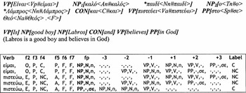
The example in Figure 1 demonstrates how a corpus sentence is transformed into the format described above. Symbols for feature values are explained in bold in the previous paragraph. In the corpus text, within the angle brackets that follow every lexical item, are a set of characters encoding morphological information of the item and its lemma, that derive from the corpus annotation process. The asterisk before a lexical item identifies it as a headword. In the final data format the fp is in bold and the six surrounding phrases follow it from left to right (-3,-2,-1, +1,. . .). So, the first instance is for the verb ε íμα and the candidate complement is the fp NP1. In the second instance, for the same verb, the candidate complement is the fp NP2. There are only two instances for this verb because
• there are no phrases preceding it,
• the third phrase following it (consisting only of the coordinating conjunction) has not much to contribute and is disregarded altogether forcing us to consider the next phrase in the sentence. As the next phrase is a verb phrase which is not introduced by a subordinating conjunction (and therefore cannot be a dependent of the verb εiμα), it is also disregarded and no further phrases are tested. These two phrase types (determined empirically) are disregarded during the phase of instance vector formation in order to cut down on redundant information that is included in the vectors.
In the same way, for the verb φiστεv;ω we have an instance with fp NP1, an instance with fp NP2 and an instance with fp PP.
The processed corpus sentence (it is followed by its English word-for-word translation) is transformed into the five labeled instances shown. Within angle brackets appear corpus notation symbols and the word lemma separated by a dash. Va and Vp stand for active and passive verb, An, Nn and Tn for adjective, noun and article in the nominative case, Na for noun in the accusative case, C for conjunction, Sp for preposition and F for punctuation mark.

We experimented with various window sizes regarding the context of the fp, i.e. [fp], [−1, fp], [−2, fp], [−2, +1], [−3, +3]. The integers indicate the number of phrases and the signs indicate whether these precede (−) or follow (+) the fp.
The formatting described in the previous section was applied to the corpus. The class of each fp for every created instance was hand-labeled by two linguists by looking up the verb in its context, based on the detailed descriptions for complements by Klairis and Babiniotis (Reference Klairis and Babiniotis1999).
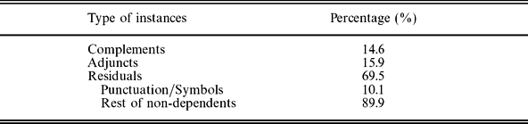
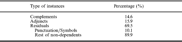
Formatting the corpora resulted in a dataset of 63,000 instances. The class imbalance ratio is 1:5.9 (one complement instance for every 5.9 non-complement instances). Among the non-complement instances, the majority is sentence constituents without content (phrases consisting of a punctuation mark only, or of a symbol, due to automatic preprocessing) and non-verb dependents that cannot be otherwise distinguished due to the low level of preprocessing. This type of phrases is called Residuals in Table 1. Symbols and punctuation constitute approximately 10% of the residuals, while the remaining 90% is other non-dependents. Adjuncts form the minority of the non-complement instances, as can be seen in Table 1.
The percentage of the types of instances in the data set
6 Addressing the class imbalance
6.1 One-sided sampling
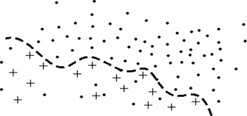
It is obvious from the ratio given above, that the complement class is underrepresented compared to the non-complement class in the data. Regarding the class of interest only, prediction of instances of the complement class suffers because of the sparseness of complements and the abundance of non-complements: as the number of examples of the majority class increases, the more likely it becomes for the nearest neighbor of a complement to be a non-complement (Figure 2). Therefore, complements are prone to misclassifications.
A graphical representation of positive and negative instances in the data.

The problem of class imbalance has been dealt with in previous work in different ways. Random oversampling (random replication of minority examples) and random undersampling (random elimination of majority examples) have been utilized to balance the class distribution (Japkowicz Reference Japkowicz2000). According to several researchers, random oversampling may lead to ovefitting, while random undersampling entails the risk of removing potentially useful data, i.e. data that is crucial for the induction process (Batista, Prati and Monard Reference Batista, Prati and Monard2004). Therefore focused resampling methods have been proposed.
Focused oversampling techniques vary from replicating only minority examples that appear in the borderline between the two classes (Japkowicz Reference Japkowicz2000), to creating new minority class examples by interpolating between existing minority examples (Chawla, Bowyer, Hall and Kegelmeyer Reference Chawla, Bowyer, Hall and Kegelmeyer2002) and approaches that combine oversampling with data cleaning (removing examples of both classes) (Batista, Bazan and Monard Reference Batista, Bazan and Monard2003).
Focused undersampling techniques vary from removing negative examples that participate in Tomek links (Tomek Reference Tomek1976), to finding a consistent subset of examples using the condensed nearest neighbor rule (Hart Reference Hart1968), and to the combination of these two approaches called one-sided sampling (Kubat and Matwin Reference Kubat and Matwin1997). Combinations of oversampling and data cleaning have also been proposed (Ling and Li Reference Ling and Li1998; Batista, Prati and Monard Reference Batista, Prati and Monard2004). One combinatory approach is to oversample the minority examples and then remove all the examples (positive and negative) that participate in Tomek links.
Another approach is the implementation of cost-sensitive classifiers, i.e. classifiers that do not treat all misclassification costs as equal (Domingos Reference Domingos1999). Provost and Fawcett (Reference Provost and Fawcett2001) present the ROC convex hull method and try to separate classification performance from class and cost distribution. Boosting is another approach that deals with imbalanced datasets (Schapire Reference Schapire2002; Guo and Viktor Reference Guo and Viktor2004) by forcing the learning algorithm to focus on hard examples (erroneously labeled examples). The algorithm places iteratively increasing weights to the misclassified examples and decreasing weights to the correctly classified ones.
Recent surveys regarding the solutions to the class imbalance problem can be found in (Batista, Prati and Monard Reference Batista, Prati and Monard2004; Weiss Reference Weiss2004), showing that different methodologies perform differently on different datasets and for different learning algorithms. We address this problem with one-sided sampling, i.e. pruning out redundant non-complement (negative) examples while keeping all the complement (positive) examples. We chose this particular sampling method because it combines one-sided cleaning of the data by removing noisy negative instances (while the minority class examples, that are rare and valuable, remain intact) using Tomek links, and removing unnecessary negative examples to even up the examples of the two classes. Random oversampling leads to serious overfitting problems in our task. Our dataset consists of nominal attributes only, most of which take a large number of values (for example the third attribute for each phrase takes sixty seven distinct values). Moreover, due to the high imbalance ratio, the positive class instances would need to be replicated several times in order for the distribution of the two classes to become balanced, causing an even bigger overfitting problem. Some experiments have been performed showing comparative results with random oversampling, boosting and one-sided sampling. They are described in detail in section 8.5.
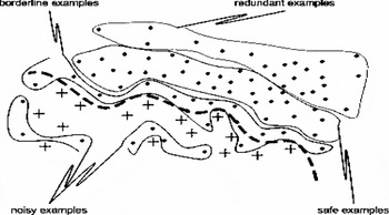
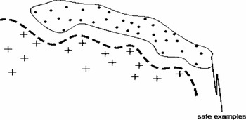
The primary goal of the proposed methodology is to end up with a representative training set where each class distribution will not suffer from disproportions. One-sided sampling has been applied to experiments in various machine learning research studies: in text classification (Lewis and Gale Reference Lewis and Gale1994), in detecting oil spills in satellite radar images (Kubat and Matwin Reference Kubat and Matwin1997), in detecting human face patterns in cluttered scenes (Sung and Poggio Reference Sung and Poggio1995), in medical applications (Laurikkala Reference Laurikkala2001). In order to obtain a representative dataset, we applied a selection technique called Tomek links, that was first introduced by Tomek (Reference Tomek1976). In the past, Kubat, Pfurtscheller and Flotzinger (Reference Kubat, Pfurtscheller and Flotzinger1994) have applied this methodology for classifying sleep stages. The basic idea behind Tomek links is that instances of the majority class can be categorized into four groups (Figure 3):
• Noisy: Instances that appear within a cluster of examples of the opposite class.
• Borderline: Instances that are close to the boundary region between two classes.
• Redundant: Instances that can be already described by other examples of the same class.
• Safe: Instances crucial for determining the class.
Instances belonging to one of the three first groups need to be eliminated as they do not contribute to class prediction.
The four groups of the majority class instances.

Redundant instances may be removed by creating a consistent subset of the initial training set. A subset S of the initial training set T is consistent with T, if, when using a learning algorithm, it correctly classifies all the instances in T. To this end we start with a subset S consisting of all complement examples and one randomly chosen non-complement example. We then train a 1-NN learner with S and try to classify the rest of the instances of the initial training set. 1-NN is the instance-based learning algorithm, where each test instance is labeled according to the label of the training instance that is closest to it (nearest neighbor) (see section 7.1). All misclassified instances are then added to S, which is a smaller, consistent subset of T. This procedure is based on the technique invented by Hart (Reference Hart1968).
Noisy and borderline examples can be detected using Tomek links: A Tomek link is formed by a pair of mutual nearest neighbors of the opposite class. All negative instances in S that participate in Tomek links are removed.
The resulting set is the final reduced training set (Figure 4). The exact process of the algorithm (Kubat and Matwin, Reference Kubat and Matwin1997) follows next:
The reduced training set, containing only positive and safe negative examples.

6.2 Distance calculations for detecting Tomek links
One drawback of the Euclidean distance, which has been traditionally used in one–sided sampling to detect examples participating in Tomek links, is that it is not very flexible regarding nominal attributes. Their distance is 0 in case they are identical and 1 in case they differ.
In our approach all attributes are nominal. The value difference metric (VDM) (Stanfill and Waltz, Reference Stanfill and Waltz1986) is more appropriate for this type of attributes, as it considers two nominal values to be closer if they have more similar classifications, i.e. more similar correlations with the output class. The VDM of two values ax and ay of a nominal attribute A in two vectors x and y can be estimated as:
where:
NA,a denotes the number of times value a of attribute A was found on the training set.
NA,a,c denotes the number of times value a of attribute A cooccurred with output class c.
C is the set of class labels
6.3 The reduced dataset
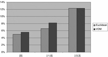
Using the above distance metrics to detect negative instances that are safe to remove, we applied the methodology of section 6.1 to the data. The graphs in Figure 5 depict the reduction in the number of negative instances in the dataset for both distance metrics and various fp context window sizes (x axis). The more phrases are taken into consideration (the higher the dimension of the vector), the noisier the instance, which leads to the removal of more redundant examples.
Reduction (%) in the number of negative instances after applying one-sided sampling with the Euclidean distance and with VDM.

It is interesting to observe, from a linguistic point of view, the type of instances which are removed from the initial dataset by balancing the two classes. Redundant instances are usually those with an fp headword a punctuation mark, a symbol etc. Such fps could never constitute a complement and appear in the dataset due to errors in the automatic nature of preprocessing. Redundant instances are also formed by fps with certain prepositions (like εφi, which can be translated as above, across, for, on or upon) or types of adverbs (like temporal) that almost never constitute complements.
Noisy and borderline instances are usually formed by fps that have a syntactically ambiguous headword like a noun in the accusative case (which is just as often a complement or a non-complement), an adjective in the nominative case if the verb is copular, certain prepositional phrases (like σ ε (to), με (with), Γiα (for)) and certain conjunctions (like nu α (to),ioτ (that)) that also function just as often as adverbial and as complements.
With the VDM metric and the [−3,+3] fp context window 73.2% of the removed negative instances were noisy and borderline and 26.8% were redundant. With the Euclidean distance, the percentage of removed noisy and borderline examples increases slightly (78.4%). To explain the difference between the two distance metrics, we take for example the following negative instance of the initial training file (with fp window size [fp]).
This instance appears only as negative throughout the whole dataset. If the verb α nu τkαθστω (to replace) is omitted, the remaining instance appears several times in the data as positive with a variety of other verbs. The Euclidean distance between these instances is small, while the VDM is greater, because the verb is a feature with a high correlation to the output class. Consequently, the above instance is removed in the reduced subset with the Euclidean distance as being borderline, while it correctly remains untouched with the VDM metric. In other words, VDM takes into account the significance of each feature for predicting the class label (the verb lemma, in the previous example, is an important feature for class prediction) and treats the previous example as safe (and not as borderline like with the Euclidean distance) and does not remove it (its VDM distance is greater that its Euclidean distance).
7 Classifying new instances
The set of learning algorithms that are used to classify new, unseen instances are described in this section. The motivation behind the selection of the algorithms is purely research-centered: to cover several machine learning fields and to compare their results on the same task and dataset. Most of the learners (instance-based learning, decision trees, Naïve Bayes, Bayesian networks) have been broadly used in several domains and their performance is well-known. A variation of Bayesian networks, COr-BBNs (Maragoudakis et al., Reference Maragoudakis, Fakotakis and Kokkinakis2004), that is more suitable for classification than Bayesian networks, is proposed and tested on the present application. Unlike previous approaches that test their methodology on only a few new verb examples, we performed tenfold cross validation on all the data. The dataset was divided into ten sets of equal size. Nine sets were used for training, and one for testing. One-sided sampling was performed on the training set only. Ten tests were run, each time using one of the ten sets for testing and the remaining nine sets for training. The results were averaged. Moreover, in order to avoid overestimation of the generalizability of a learner caused by cross validation, we also perform experiments using a held-out test set.
7.1 IB1
IB1 is the simplest instance-based learning algorithm (Aha, Kibler and Albert Reference Aha, Kibler and Albert1991). It is identical to the nearest-neighbor algorithm (1-NN). The value ranges of all n attributes are normalized and all the attributes have the same impact on classification (are considered to be equally significant). The distance between the values ax and ay of attribute A in instances x and y is calculated as
and the distance between two vectors is calculated as
Each new unseen test instance is labelled with the class of the training instance which is nearest (has the smallest distance) to it.
7.2 Weighted IB1
Apart from the traditional IB1 (1-NN algorithm), we experimented with a weighted version, where each feature A is weighted with its information gain (IG) (Quinlan Reference Quinlan1993). Thereby we express the average reduction in the training set information entropy, when knowing the value of the feature. Each weight is calculated by the following equation.
C is the set of class labels, V A is the set of values a for feature A and H(C) is the entropy of the class labels:
7.3 Decision trees
We use an implementation of the C4.5 decision tree learner (Quinlan Reference Quinlan1993) in the classification experiments. Reduced error pruning (Quinlan Reference Quinlan1993) is performed and one of the ten data subsets is used as the held-out validation set for guiding the pruning process. Due to the use of word lemmata as feature values, pruning is necessary. Otherwise the size of the tree grows very large and the problem of overfitting becomes very significant.
7.4 Naïve Bayes
The Naïve Bayes classifier performs inference by applying Bayes rule to compute the posterior probability of a class C, given a particular vector of n input variables Ai, i=1 to n. It then outputs the class whose posterior probability is the highest. Regarding its computational cost, inference in Naïve Bayes is feasible, due to two assumptions, yet often unrealistic for real world applications:
• All the attributes A i are conditionally independent of each other, given the classification variable.
• All other attributes are directly dependent on the class variable.
Despite the fact that Naïve Bayes performs well in several applications (Domingos and Pazzani Reference Domingos and Pazzani1997), it is counterintuitive to ignore the correlation of the variables in some domains.
7.5 Bayesian belief networks
Bayesian belief networks (BBN) provide a comprehensive means for effective representation of independence assumptions (Pearl Reference Pearl1988). Given a set of attributes A = A 1,. . ., A n, where each variable A i could take values from a finite set, a Bayesian network describes the probability distribution over this set of variables.
If one of the nodes is the target class (Cl), the Bayesian network returns the most probable class label, which maximizes the posterior probability P B(Cl/A 1,. . . A n).
However, Friedman and Goldszmidt (Reference Friedman and Goldszmidt1996) have proved that general, unrestricted Bayesian networks may not be good classifiers. They justify this by observing that learning a Bayesian network structure is unsupervised in the sense that no distinction is made among the class node and the other attribute nodes. In other words, since the class node is not explicitly stated, the structure – or some part of it – may not be relevant for classification, if it is outside the Markov blanket of the class node. Pearl (Reference Pearl1988) defined the Markov blanket of a node X as the union of X's direct parents, X's direct children and all direct parents of X's children. The semantic notion of the Markov blanket is that X is unaffected by nodes outside its Markov blanket. The Markov blanket is influenced by the directionality of the arcs in the network. For classification tasks, if the Markov blanket of the class node (i.e. the node whose values is to be predicted) contains limited nodes, then the accuracy is prone to errors. On the other hand, if the Markov blanket of the class contains all the other nodes (i.e. all other variables) then it might also lead to classification errors, since some variables may not necessarily be dependent of the class.
In the next section, we describe a Bayesian network structure that augments the Markov blanket of the class variable with only relative nodes, providing networks that favour the classification process.
7.6 Class-oriented Bayesian networks
It is more than obvious that a network structure is needed that will accurately reflect the distribution of the attributes of a domain. Additionally, it should also perform well when it comes to classification. We propose an algorithm for learning Bayesian networks from data with a classification-oriented structure. This type of network is called Class-oriented Bayesian belief network or ‘COr-BBN’. COr-BBNs were first presented in detail in (Maragoudakis et al. Reference Maragoudakis, Fakotakis and Kokkinakis2004) and are suitable for classification since they retain the probability distribution of the domain and they also perform a feature selection for the given class. Unlike the unsupervised approach of the BBN learning technique, a COr-BBN knows the class prior to learning its structure and forces a potential arc from an attribute to the class to be reversed. By this approach, the class is always the cause of an attribute. By imposing restrictions as regards to the direction of arcs, we can actually learn the optimal set of attributes that belong to the Markov blanket of class Cl.
8 Experimental results
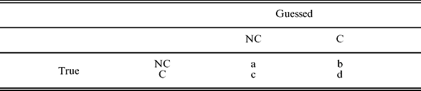
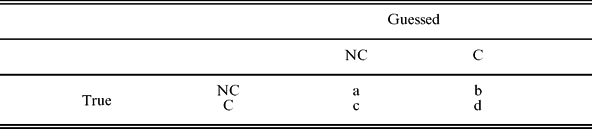
The results we obtained are evaluated according to the metrics which can be derived from the confusion matrix in Table 2. The rows correspond to the true classes while the columns correspond to the classes assigned by the classifier. More specifically the metrics used are:
Precision and recall are used in a standard way in this paper, but they are defined here for each class so as not to cause any confusion.
Confusion matrix. The rows represent the actual classes and the columns the predicted classes
The f-measure for each class combines the previous two metrics into one and is calculated as follows:
8.1 Results with the initial dataset
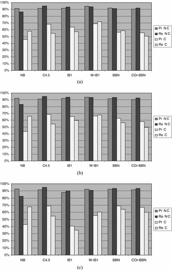
Figure 6 shows the results for every classification algorithm and various fp context window sizes using the initial dataset before any attempt is made to reduce its size. Regarding the instances of both classes, accuracy (the number of correctly identified instances divided by the total number of instances) is high due to the large number of correctly classified non-complements. However, the drop in precision and recall of the minority class compared to those of the majority class is obvious. Instance-based and decision tree learning outperform the rest of the methods for the small fp context window sizes. By explicitly storing and taking into account every training example, the former presents a drop in performance as the window size increases due to sparse data. The performance of C4.5, however, remains stable regardless of the size of the instance vector determining the attributes by taking into account the impact of each attribute on classification. The longer the instance vector (the bigger the context window), the more likely it is to contain irrelevant information. By nature, weighted IB1 also takes into account the relevance of each attribute and therefore presents a smaller drop in performance as the window gets bigger. Naïve Bayes leads to a significant number of non-complement instances being labeled as complements. This is attributed to the fact that the Naïve Bayes learner does not take into account conditional dependencies among features (all the features are considered independent given the class). Given that an instance is a complement, for example, if the fp is an adjective in the nominative case, there is a very high probability in reality that the verb is copular. This dependence is not captured by the Naïve Bayes learner. BBNs and COr-BBNs have achieved a higher precision for the minority class compared to Naïve Bayes, with BBN presenting the highest f-measure of the three. The best complement class f-measure is achieved by weighted IB1 (70.3%) when no fp context is taken into account (fp context window [fp]).
Results for both classes with the initial dataset for every classifier and fp context window [fp] in (a), [−1,fp] in (b) and [−3,+3] in (c).

8.2 Results with the reduced dataset
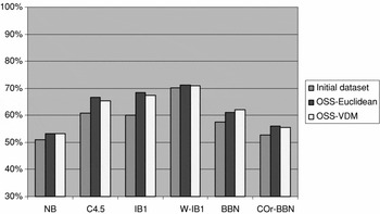
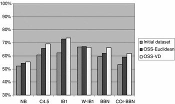
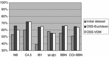
Figures 7–9 show in detail comparative results before and after balancing the dataset for the complement class as this is the class of interest. The increase in performance after reducing the dataset is very interesting to observe and depends on the size of the fp context window.
F-measure for the minority class with the initial dataset, the reduced dataset using the Euclidean distance (OSS-Eucl) and the reduced dataset using the VDM (OSS-VDM), with fp context window [fp].

F-measure for the minority class with the initial dataset, the reduced dataset using the Euclidean distance (OSS-Eucl) and the reduced dataset using the VDM (OSS-VDM), with fp context window [−1,fp].

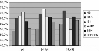
F-measure for the minority class with the initial dataset, the reduced dataset using the Euclidean distance (OSS-Eucl) and the reduced dataset using the VDM (OSS-VDM), with fp context window [−3,+3].

When taking into account the context surrounding the fp, the positive impact of balancing the dataset is even stronger. As the fp window size increases, Naïve Bayes performs better, reaching an f-measure of over 60% with [−3,+3] (as opposed to 53.4% prior to balancing). The Bayesian network learners, whose performance was mediocre when no context was taken into account, also achieve higher results when including full context, reaching over 68% with BBN and 66% with COr-BBN. The highest scores for both these methods prior to balancing are 55% and 51% respectively. C4.5 results are improved by almost 12% in context [−3,+3] after balancing compared to the results obtained before balancing. With smaller context, increase with C4.5 ranges between 9% and 10%. Instance-based learning, as mentioned earlier is not helped by a lot of context information and reaches its highest score when considering only one phrase preceding the fp. The increase in the IB1 f-measure, however, is almost 22% and is the biggest performance improvement achieved in the experiments. The removal of the noisy and redundant examples seems to compensate for the noise introduced by the increased number of features in the vector. The highest f-measure (73.7%) is achieved by IB1 for context window [−1, fp] with subset learner IB1 and VDM distance corresponding to a precision of 77.5% and a recall of 70.3%. Precision and recall for the non-complement class are 93.8% and 95.6%, respectively (94.7% f-measure).
As can be seen in most of the experiments, and with only a few exceptions, VDM leads to better results than the Euclidean distance, as expected, because it is more appropriate for nominal features as was explained in detail in sections 6.2 and 6.3.
In several cases, BBNs and COr-BBNs lead to the same results. That is because, given a training set, it may occur that any interconnections between the class node and the other variable nodes are directed from the class to the variables, due to the probability distribution that governs this set. Whenever the COr-BBN algorithm is called over the same set, no direction restrictions would have to be posed since the arcs are already classification-oriented.
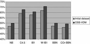
In order to evaluate the experimental methodology, Figure 10 shows the results that were achieved using not 10-fold cross validation, but a held-out test set for evaluation. In these experiments 90% of the dataset was used for training and 10% for testing. The dataset was split at random. Sampling was performed on the training set only. The increase in complement class prediction performance is not affected. Compared to the tenfold cross validation, the results for some classifiers are slightly lower with the held-out test set due to the small number of test instances.
F-measure for the minority class with the initial dataset, and the reduced dataset using the VDM (OSS-VDM), with fp context window [−1,fp] when using a held-out test set.

8.3 Resolution of ambiguities
Concerning the resolution of ambiguities discussed in section 2, three classified examples ([−1,fp]) of the verb ασkω (to exercise) follow. The first class label is the true class and the second is the predicted class. Example (a) has been classified correctly with and without one-sided sampling, examples (b) and (c) are the same instance classified without (b) and with (c) one-sided sampling. (b) is erroneously tagged as an non-complement due to class imbalance. The phrase preceding the fp helps raise the complement/non-complement ambiguity in (a) and (c): usually a punctuation mark preceding the fp (indicated by the triple NP,F,- in (a)) separates syntactically the fp from the verb and the fp is unlikely to constitute a complement.
Another example of ambiguity resolution is the following, where the verb θε τω (to set, to pose, to put) has an fp a PP with preposition σε. (d) shows the erroneous classification of the instance as a non-complement, when using the initial training set, due to the large number of non-complement examples in the training set with the same fp. (e) shows the correct classification when training with the reduced dataset. Most of the nearest neighbors in (e) are found to be complements, while in (d) they are non-complements. One-sided sampling helps resolve the ambiguity of this type of fp.
8.4 Indicatory networks
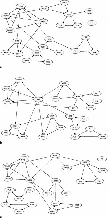
The learned Bayesian belief networks over the data are depicted in Figures 11 and 12 to show the dependence among attributes and their relevance to the classification task at hand. In Figure 11, the dataset for these networks is with fp context [−2,+2]. The networks of this context window were chosen to be shown, despite the fact that results with this window size have not been displayed, because the number of features with this size is optimal to show dependencies between them: not too small that important information is by-passed and not too large containing many features that are not related to the others. (The features of the third phrase preceding and following the candidate complement show no relation to the rest of the features, or the class). In (a) the network has been learned by the initial dataset, in (b) and (c) it has been learned from the reduced (using BBNs for classification) dataset using the VDM and the Euclidean distance respectively. LABEL is the node corresponding to the classification label (complement/non-complement), VERB is the verb lemma, FOCUSi, i=1 to 3, is the node corresponding to the ith fp feature, PLij, i, =,1 to 2, j=1 to 3, corresponds to the jth feature of the ith phrase following the fp. MINij corresponds to the jth feature of the ith phrase preceding the fp. Nodes PA and PG represent the presence or not in the verb phrase of a pronoun in the accusative or the genitive case, respectively. COP describes the verb's copularity, PERS is the node determining whether the verb is (im)personal, and VOICE and Mode determine obviously the voice and mode of the verb. Using the Euclidean distance, the phrases following the fp do not seem to affect complement identification at all. With VDM, feature relevance changes and more features play a major (the fp, the immediate context around the fp, the verb's mode and voice) or minor (the more distant context, PA, PERS) role in classification. The more distributed dependence leads to VDM producing better results in most experiments. The relevance of PG to the task has remained undetected with this method, as it appears without links to any other node in all three networks. It can also be deduced from the networks that the phrases preceding the fp are more significant for classification than the ones following it. This has also been shown with IB1, which achieves its best scores with context [−1, fp].
In Figure 12, the BBN and COr-BBN networks for the dataset with context window [−1, fp] are shown. It is interesting to observe that the number of nodes that have a direct connection to the class node increases after one-sided sampling (6 vs. 5). In other words, the significance of the immediate context around the fp is more easily recognizable after balancing, and leads to better classification performance. Also, the graphs show the difference between BBNs and COr-BBNs: the difference in the direction of the arcs of the class node.
The most probable Bayesian belief networks over (a) the initial, (b) the reduced by VDM and (c) the reduced by the Euclidean distance [−2,2] datasets.

The most probable Bayesian belief networks over the initial dataset with BBNs (a), COr-BBNS (b), and the reduced dataset with VDM with BBNs (c) and COr-BBNs (d). The dataset in these networks is with context window size [−1, fp].

8.5 Comparative results with various balancing approaches
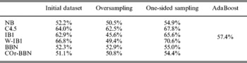
As was mentioned in section 6.1, indicatory experiments have been carried out in order to compare the performance of various approaches to the class imbalance problem, apart from one-sided sampling. One methodology included in these experiments is random oversampling, where the minority class examples are replicated as many times as is needed in order for the distribution of the two classes to become balanced. Another approach is boosting. We chose AdaBoost (Schapire Reference Schapire2002), the most commonly used boosting algorithm. AdaBoost is an iterative algorithm that puts weights on the training examples and modifies these weights in each iteration, depending on whether a training example is or isn't associated with misclassifications. Thereby AdaBoost forces the base learner (the learning algorithm that is repeated iteratively) to focus on the difficult examples. In our experiments we chose IB1 as the base learner. The experiments were performed using the training set and held-out test set described at the end of section 8.2. The results for a [−1, fp] context environment window are shown in Table 3. One-sided sampling outperforms the other approaches by combining one-sided data cleaning (removing only negative examples that participate in Tomek links while keeping all the positive examples) and undersampling (removing all the unnecessary negative examples). The unnecessary negative examples are abundant due to the low level of preprocessing, as explained earlier in this work. Therefore, this sampling method, by removing unnecessary as well as misleading negative examples, proves to be the most appropriate one for the present task.
Complement class f-measure for every classification algorithm and various approaches to class imbalance. The context window size is [−1,fp]. The base learner for AdaBoost is IB1

8.6 Summary of results
The main outcome of the work described in this paper is the increase in complement-class f-measure up to 22% by removing unnecessary and misleading non-complement examples. The highest results we achieved were 77.5% precision and 70.3% recall (73.7% f-measure), when taking into account only the context of one phrase preceding the fp, showing thereby that context information is important to some extent, but when the window size grows too large, it becomes misleading. VDM proved to be more appropriate for the present labeling application because the latter is described exclusively by nominal features. Instance-based learning performs best when the context window surrounding the candidate complement is very restricted (at most one phrase preceding the focus phrase), while Bayesian learning improves its performance as the context window size increases.
Learning verb complements is not a novel task. However, making use of so limited resources to perform the task allows the proposed methodology to be applied to the plethora of languages that are not rich in resources. Moreover, the idea to apply one-sided sampling, in order to balance the noisy dataset, on a computational linguistics task is novel. Novel is also the incorporation of the VDM metric in the sampling methodology to determine the examples that are safe to remove. The comparative results for so many and different machine learning algorithms on the same dataset is also a very interesting part of the present work, as well as their comparative reaction when the size of the learning vector increases. Last, but not least, an important novelty of the present work is the language itself. Modern Greek is a less widely spoken language and, as a result, it is relatively poor in resources and the research done on it is limited. Dealing with such a language is an interesting endeavor on its own.
Figure 13 shows a summary of the most important results: the complement class f-measure for all learning algorithms, fp context windows after applying one-sided sampling with VDM.
A summary of results: Complement class f-measure for all learning algorithms and fp context windows (OSS-VDM).

9 Conclusion
In this paper we have described the positive effect of one-sided sampling for the first time on the automatic detection of verb complements from Modern Greek text corpora. Due to the unavailability of sophisticated linguistic resources for preprocessing the data, the amount of noise (non-complements) in the learning examples is high, and the disproportion between positive (complement) and noisy instances leads to a drop in performance. Unlike traditional one-sided sampling, we employed the value difference metric as well as the Euclidean distance and showed that the former is more appropriate when dealing with nominal features. We carried out extensive experiments with a number of well-known machine learning algorithms (instance-based learning, decision trees, Bayesian learning) in order to classify new examples of complement candidates, having merely made use of a phrase chunker and basic morphological information for preprocessing.