


Introduction
Strategic sowing of two or more crops in space (row intercropping, strip intercropping and mixed intercropping) and time (relay intercropping) in the same field is called intercropping (Dordas et al., Reference Dordas, Vlachostergios and Lithourgidis2012). It is mainly practised in developing countries under low inputs agricultural systems but also getting popular in developed countries (Dordas et al., Reference Dordas, Vlachostergios and Lithourgidis2012; Lithourgidis et al., Reference Lithourdigis, Dordas and Vlachostergios2011). Intercropping has multi-dimensional advantages such as improved yield on sustained basis (Lithourgidis et al., Reference Lithourdigis, Dordas and Vlachostergios2011; Mao et al., Reference Mao, Zang, Li, van der Werf, Sun, Spiertz and Li2012) and better resource use efficiency, i.e. land use efficiency (Agegnehu et al., Reference Agegnehu, Ghizaw and Sinebo2008; Feike et al., Reference Feike, Chen, Penning, Graeff-Honninger, Zuhlke, Claupein, Darnhofer and Grotzer2010; Szumigalski and van Acker, Reference Szumigalski and van Acker2006), water use efficiency (Mao et al., Reference Mao, Zang, Li, van der Werf, Sun, Spiertz and Li2012; Siddique et al., Reference Siddique, Regan, Tennant and Thomson2001), nutrient use efficiency (Hauggaard-Nielsen et al., Reference Hauggaard-Nielsen, Ambus and Jensen2001; Zhang and Li, Reference Zhang and Li2003; Zhang et al., Reference Zhang, van der Werf, Zhang, Li and Spiertz2007), radiation use efficiency (Tsubo et al., Reference Tsubo, Walker and Mukhala2001; Zhang et al., Reference Zhang, van der Werf, Bastiaans, Zhang, Li and Spiertz2008) etc. Other benefits include soil conservation (Mushagalusa et al., Reference Mushagalusa, Ledent and Draye2008; Zougmore et al., Reference Zougmore, Kambou, Ouattara and Guillobez2000), weed control (Banik et al., Reference Banik, Midya, Sarkar and Ghose2006), disease control (Sikirou and Wydra, Reference Sikirou and Wydra2008), beneficial insects attraction in organic agriculture (Jones and Gillett, Reference Jones and Gillett2005) and high economic benefits to growers (Ali et al., Reference Ali, Khan, Ahmad and Ali2006; Khan et al., Reference Khan, Khan, Hussain, Farooq, Jabran and Lee2012; Malézieux et al., Reference Malézieux, Crozat, Dupraz, Laurans, Makowski, Ozier-Lafontaine, Rapidel, de Tourdonnet and Valantin-Morison2009; Mucheru-Muna et al., Reference Mucheru-Muna, Pypers, Mugendi, Kung, Mugwe, Merckx and Vanlauwe2010). Hence, intercropping is considered as a promising system that results in an effective use of land and other resources and reduction in cost of production.
In intercropping systems, differences may occur between the component crops in competitive ability for growth resources. Yield advantage occurs because growth resources such as light, water and nutrients are more efficiently absorbed and converted to biomass by the component crops over time and space. Normally, complementary use of resources occurs when the component crops of an intercropping system use different resources or they use the same resources at different places or at different times. This results due to the variation in characteristics of component crops such as rates of vegetative growth, final canopy size, photosynthetic adaptation of canopies to prevailing light conditions and nature of root system, including rooting depth (Tsubo et al., Reference Tsubo, Walker and Mukhala2001).
Selection of crops differing in competitive ability in time or space is essential for an efficient intercropping system as well as making decisions on planting time, density and arrangement. Thus, crop management decisions specify the design of intercropping systems, and its performance is governed largely by the availability and the competition for growth resources. Legumes can fix atmospheric nitrogen, changing it from an inorganic form to forms that are available for uptake by plants through symbiotic association with some nitrogen fixing bacteria, and hence improve soil fertility and results in sustainable crop production. Biological fixation of atmospheric nitrogen can replace nitrogen fertilization wholly or in part. Legumes grown in intercropping are regarded as an alternative and sustainable way of introducing nitrogen into lower input agro-ecosystems (Fustec et al., Reference Fustec, Lesuffleur, Mahieu and Cliquet2010). In addition, the green parts and roots of the legume component decompose and release nitrogen and other nutrients into the soil, where these may be made available to subsequent crops. Intercropping involving legumes has gained wide acceptability among farmers of tropical and sub-tropical countries. It has also been found to be most useful (Adeniyi, Reference Adeniyi2011) because of its economic advantages resulting from nitrogen fixing activity of legumes intercropped with other crops.
In the present study, pea (Pisum sativum) was selected due to its high nitrogen fixing activity and importance as a vegetable. Other vegetables such as garlic (Allium sativum), turnip (Brassica rapa) and cauliflower (Brassica oleracea) were intercropped with peas because of their nutritional and commercial importance in the country. Using pea in intercropping systems, two vegetables can be grown by the same growth resources, hence reducing the cost of production. The current research involving intercropping pea with other non-legume winter vegetables (i.e. garlic, turnip and cauliflower) was envisaged to evaluate advantages of intercropping systems through competition and economic indices.
Materials and Methods
Crop management and experimental design
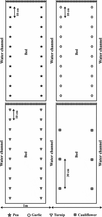
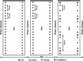
The present study was conducted at the Vegetable Research Area, Department of Horticulture, Bahauddin Zakariya University, Multan, Pakistan to determine the intercrop competition between pea and three non-legume winter vegetables and economics of each intercropping system. The experiment was conducted during 2010–2011 (November to May) and repeated during 2011–2012. The soil used for the experiment was loamy with pH 8.03, electrical conductivity (EC) 1.80 dSm−1, organic matter 0.37%, available phosphorus 4.75 ppm and potassium 140 ppm. According to the US Department of Agriculture (USDA) classification, the soil belonged to Sindhlianwali soil series (fine silty, mixed, hyperthermic, sodic haplocambids). The vegetable crops included in the study were pea (cv. Early 6), garlic (cv. GS-1), turnip (cv. Purple Top) and cauliflower (Hybrid RS 5340). All these vegetable crops were grown alone as monocrops and later three vegetables in combination with pea as intercrops. The experiment was laid out according to randomized complete block design (RCBD) with three replications. Seeds of pea and turnip and cloves of garlic were planted and one-month old seedlings of cauliflower were transplanted on 5th November during both the years, i.e. 2010 and 2011, on beds, keeping bed-to-bed distance of 1 m. Each experimental plot had three beds and each bed was 1-m wide and 4-m long with an area of 12 m2. In monocroping, the planting distances kept for pea, garlic and turnip were 10 cm, and for cauliflower the planting distance was 30 cm (Figures 1 and 2). The same planting distances were maintained in intercropping treatments. Phosphorus (P2O5) and potassium (K2O) were applied to all at the rate of 90 and 50 kg ha−1 respectively at sowing. Nitrogen was applied at a rate of 90 kg ha−1 in three split doses: 1/3 at sowing, 1/3 after one month of sowing and remaining 1/3 after first picking of peas. No additional dose of any fertilizer was applied to the intercrops. All other cultural practices, such as irrigation, hoeing, thinning out and plant protection measure, were uniform for all the experimental plots during both the years.
Planting geometry of monocropping systems.

Planting geometry of pea-based intercropping systems.

Data collection
Plants were allowed to grow till edible maturity and then harvested and their vegetable yields (economic yields) and total biomass (biological yields) were recorded. However, for pea, data of all pickings of pods were added to estimate total pod yield. Harvest index (HI) was calculated by using the following formula:
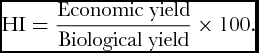 \begin{equation*}
{\rm HI} = \frac{{{\rm Economic}\;{\rm yield}}}{{{\rm Biological}\;{\rm yield}}} \times 100.
\end{equation*}
Competition indices
-
1. Land equivalent ratio (LER) was calculated by the formula given by Willey (Reference Willey1979):
where \begin{equation*}
{\rm Total}\;{\rm LER} = {\rm LER}_{{\rm pea}} + {\rm LER}_{{\rm intercrop}} ,
\end{equation*}
\begin{equation*}
{\rm LER}_{{\rm pea}} = \frac{{{\rm Economic}\;{\rm yield}\;{\rm of}\;{\rm pea}\;{\rm in}\;{\rm intercropping}}}{{{\rm Economic}\;{\rm yield}\;{\rm of}\;{\rm pea}\;{\rm as}\;{\rm sole}\;{\rm crop}}}{\rm , and }
\end{equation*}
\begin{equation*}
{\rm LER}_{{\rm intercrop}} = \frac{{{\rm Economic}\;{\rm yield}\;{\rm of}\;{\rm respective}\;{\rm crop}\;{\rm in}\;{\rm intercropping}}}{{{\rm Economic}\;{\rm yield}\;{\rm of}\;{\rm respective}\;{\rm sole}\;{\rm crop}}}.
\end{equation*}
-
2. Relative crowding coefficient (K) was computed as suggested by DeWit (Reference DeWit1960):
where
\begin{equation*}
K = K_{{\rm pea}} \times K_{{\rm intercrop}} ,
\end{equation*}
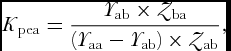
\begin{equation*}
K_{{\rm pea}} = \frac{{Y_{{\rm ab}} \times Z_{{\rm ba}} }}{{\left( {Y_{{\rm aa}} - Y_{{\rm ab}} } \right) \times Z_{{\rm ab}} }},
\end{equation*}\vspace*{-12pt}
where Y aa is pure stand yield of pea crop, Y ab is intercrop yield of pea, Y bb is pure stand yield of component intercrop, Y ba is intercrop yield of component intercrop, and Z ab and Z ba are sown proportions of pea and component intercrops in intercropping systems.
\begin{equation*}
K_{{\rm intercrop}} = \frac{{Y_{{\rm ba}} \times Z_{{\rm ab}} }}{{\left( {Y_{{\rm bb}} - Y_{{\rm ba}} } \right) \times Z_{{\rm ba}} }},
\end{equation*}
-
3. Aggressivity (A) value was calculated following the formula of McGilchrist (Reference McGilchrist1965):
\begin{equation*}
A_{{\rm pea}} = \left( {\frac{{Y_{{\rm ab}} }}{{Y_{{\rm aa}} \times Z_{{\rm ab}} }}} \right) - \left( {\frac{{Y_{{\rm ba}} }}{{Y_{{\rm bb}} \times Z_{{\rm ba}} }}} \right),
\end{equation*}\vspace*{-12pt}
\begin{equation*}
A_{{\rm intercrop}} = \left( {\frac{{Y_{{\rm ba}} }}{{Y_{{\rm bb}} \times Z_{{\rm ba}} }}} \right) - \left( {\frac{{Y_{{\rm ab}} }}{{Y_{{\rm aa}} \times Z_{{\rm ab}} }}} \right).
\end{equation*}
-
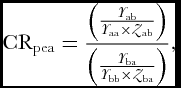
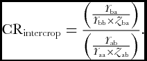
4. Competitive ratio (CR) was calculated by using the formula of Willey et al. (Reference Willey, Natarajan, Reddy, Rao, Nambiar, Kammainan, Bhatanagar and Homeless1980):
\begin{equation*}
{\rm CR}_{{\rm pea}} = \frac{{\left( {\frac{{Y_{{\rm ab}} }}{{Y_{{\rm aa}} \times Z_{{\rm ab}} }}} \right)}}{{\left( {\frac{{Y_{{\rm ba}} }}{{Y_{{\rm bb}} \times Z_{{\rm ba}} }}} \right)}},
\end{equation*}\vspace*{-12pt}
\begin{equation*}
{\rm CR}_{{\rm intercrop}} = \frac{{\left( {\frac{{Y_{{\rm ba}} }}{{Y_{{\rm bb}} \times Z_{{\rm ba}} }}} \right)}}{{\left( {\frac{{Y_{{\rm ab}} }}{{Y_{{\rm aa}} \times Z_{{\rm ab}} }}} \right)}}.
\end{equation*}
-
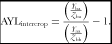
5. Actual yield loss (AYL) was calculated by the formula of Banik (Reference Banik1996):
\begin{equation*}
{\rm AYL} = {\rm AYL}_{{\rm pea}} + {\rm AYL}_{{\rm intercrop}} ,
\end{equation*}\vspace*{-12pt}
\begin{equation*}
{\rm AYL}_{{\rm pea}} = \frac{{\left( {\frac{{Y_{{\rm ab}} }}{{Z_{{\rm ab}} }}} \right)}}{{\left( {\frac{{Y_{{\rm aa}} }}{{Z_{{\rm aa}} }}} \right)}} - 1,
\end{equation*}\vspace*{-12pt}
\begin{equation*}
{\rm AYL}_{{\rm intercrop}} = \frac{{\left( {\frac{{Y_{{\rm ba}} }}{{Z_{{\rm ba}} }}} \right)}}{{\left( {\frac{{Y_{{\rm aa}} }}{{Z_{{\rm bb}} }}} \right)}} - 1.
\end{equation*}









Economic and monetary advantages
-
1. Intercropping advantage (IA) was calculated by using the formula of Banik et al. (Reference Banik, Sasmal, Ghosal and Bagchi2000):
\begin{equation*}
{\rm IA}_{{\rm pea}} = {\rm AYL}_{{\rm pea}} \times P_{{\rm pea}} ,
\end{equation*}\vspace*{-18pt}
\begin{equation*}
{\rm IA}_{{\rm garlic}} = {\rm AYL}_{{\rm garlic}} \times P_{{\rm garlic}} ,
\end{equation*}\vspace*{-18pt}
\begin{equation*}
{\rm IA}_{{\rm turnip}} = {\rm AYL}_{{\rm turnip}} \times P_{{\rm turnip}} ,
\end{equation*}\vspace*{-18pt}
where P is the commercial value of the respective crop. The prevailing prices of pea, garlic, turnip and cauliflower were US$ 400, 1000, 100 and 200 per tonne respectively.
\begin{equation*}
{\rm IA}_{{\rm cauliflower}} = {\rm AYL}_{{\rm cauliflower}} \times P_{{\rm cauliflower}} ,
\end{equation*}
-
2. Monetary advantage index (MAI) was calculated by using the formula of (Ghosh, Reference Ghosh2004):
\begin{equation*}
{\rm MAI} = \frac{{\left( {{\rm Value}\;{\rm of}\;{\rm intercrops}} \right)\times \left( {{\rm LER} - 1} \right)}}{{{\rm LER}}}.
\end{equation*}
-
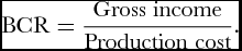
3. Net income and benefit cost ratio (BCR) was estimated to determine the feasibility of different pea intercropping systems. The production cost of intercropping systems included land rent, cost of field and seed bed preparation, seed sowing/transplanting, irrigation, fertilizers, crop protection measures and harvesting/picking. Gross income was estimated using the prevailing prices in the local market for the vegetables. Net income was calculated by subtracting the cost of production from the gross income. The BCR for each intercropping system was computed by the following formula:
\begin{equation*}
{\rm BCR} = \frac{{{\rm Gross}\;{\rm income}}}{{{\rm Production}\;{\rm cost}}}.
\end{equation*}





Statistical analysis
Data procured were analysed statistically through Co-stat statistical package software (Co-Stat 6.300, 2003) by constructing ANOVA tables. The data regarding HI (in percentage) were subjected to analysis of variance after Arcsine transformation, analysis of gross and net income (whole numbers with wide range of values) after logarithmic transformation, and analysis of land equivalent ratio, competition ratio and cost benefit ratio after log (X+1) transformation, where X is the original data value. The data having negative values were transformed by adding a constant value to make positive, data of aggressivity and actual yield loss (with small whole numbers) were subjected to square root transformation, and data of intercropping advantage (with wide range) were subjected to logarithmic transformation before analysis of variance. The mean values were compared by employing Least Significant Difference (LSD) test at p = 0.05.
Results
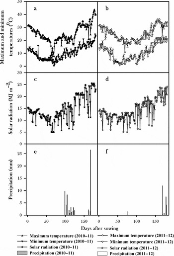
The weather conditions during the growing period in terms of daily maximum and minimum temperatures, solar radiation and precipitation during both the years, i.e. 2010–2011 and 2011–2012 are given in Figure 3. The monthly mean values of average air temperature during growing seasons of both the years were similar. In addition, there were no differences in solar radiation. During 2010–2011, maximum, minimum and average temperatures were 7.7–43.6 °C, 0.3–24.7 °C and 10.56–25.26 °C respectively, and during 2011–2012, these were 11.0–36.0 °C, 0.9–23.0 °C and 10.77–25.15 °C respectively. Solar radiation ranged from 4.98–25.52 MJ m−2 with an average of 14.75 MJ m−2 during 2010–2011, while it ranged from 4.97–24.10 MJ m−2 with an average of 14.26 MJ m−2 during 2011–2012. During 2010–2011, there was significant rainfall whereas during 2011–2012, there was lower rainfall. Maximum once rainfall was 26.6 mm and 12.00 mm, and total rainfall was 66.7 mm and 26.6 mm for 2010–2011 and 2011–2012 respectively. In spite of the fact that there were differences in precipitation between the two growing years, the ANOVA for vegetable yields indicated that there was no significant effect of year and intercropping treatments×years interaction. Therefore, data only for intercropping treatments averaged across growing years are presented.
Daily maximum and minimum temperature (a and b), solar radiation (c and d), precipitation (e and f) during 2010–2011 (filled symbols) and 2011–2012 (un-filled symbols) at Multan, Pakistan.

Crop yield and harvest index
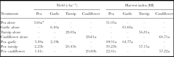
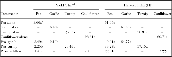
Mean vegetable yields of pea, garlic, turnip and cauliflower were significantly higher in monocrops as compared with intercrops. Among intercropping systems, highest pod yield of pea was obtained when intercropped with garlic. Pod yield significantly decreased when intercropped with turnip whereas minimum pod yield was recorded in case of pea–cauliflower intercropping system (Table 1). The reduction in pod yield of pea was 4.64% when intercropped with garlic, and 38.52% and 61.48% when intercropped with turnip and cauliflower respectively. Clove yield of garlic, root yield of turnip and curd yield of cauliflower decreased by 65.78, 29.07 and 28.00% of their monocrops respectively when these were intercropped with pea.
Effect of pea-based intercropping systems on yield and harvest index of component crops.
*Mean values sharing similar letter(s) in a column are statistically non-significant at p = 0.05 (LSD test).
Significant differences were found in HI among pea grown alone and in various combinations with non-legume winter vegetables studied. Highest HI was recorded when pea was grown alone, followed by when intercropped with pea, and both these intercropping systems were statistically similar. Harvest index of pea was significantly decreased when intercropped with turnip or cauliflower. However, these two intercropping systems were statistically different from each other and also differed significantly from former intercropping systems. Harvest indices of garlic, turnip and cauliflower when grown alone and intercropped with pea were statistically similar, indicating that these were not affected by the intercropping systems (Table 1).
Competition indices
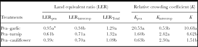
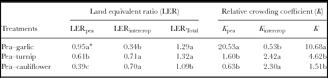
The maximum partial LERpea value was obtained when pea was intercropped with garlic, the value decreased when pea was intercropped with turnip and reached to the minimum when it was intercropped with cauliflower. All these partial LERpea values were statistically different from each other. The partial LERpea values were higher than 0.5 for pea–garlic and pea–turnip intercropping systems. However, partial LERintercrop values were higher than 0.5 for pea–cauliflower and pea–turnip intercropping systems. The values of partial LERintercrop for pea–cauliflower and pea–turnip intercropping systems were 0.72 and 0.71 respectively as compared with 0.34 for pea–garlic. The former two values were statistically similar but differed significantly from latter one. The LERtotal value was maximum in the case of pea–turnip intercropping, closely followed by pea–garlic, whereas minimum value was obtained in case of the pea–cauliflower intercropping system. The LERtotal values in the intercropping systems were 1.29, 1.32 and 1.11 for pea–garlic, pea–turnip and pea–cauliflower intercropping systems respectively (Table 2). The former two values of LERtotal were statistically similar but significantly different from the latter one. This indicates that 11–32% more area would be required for their monocropping system compared with intercropping to produce their yield achieved in the intercropping. Thus, there was a substantial land use advantage of intercropping of turnip, cauliflower and garlic with pea.
Effect of pea based intercropping systems on land equivalent ratio and relative crowding coefficient of pea, garlic, turnip and cauliflower.
*Mean values sharing similar letter(s) in a column are statistically non-significant at p = 0.05 (LSD test).
The highest relative crowding coefficient value for pea (K pea) was found for pea–garlic intercropping system (20.53) which was significantly higher than pea–turnip (1.60) and pea–cauliflower (0.63) intercropping systems. However, latter two values were statistically at par. The value of K pea was also more than 1 (1.60) for pea–turnip intercropping, while for pea–cauliflower system, it was less than 1 (0.63). For intercrops, relative crowding coefficient (K intercrop) value was higher for cauliflower (2.57), followed by turnip (2.44), which were statistically similar, and it was lowest for garlic (0.52), which was statistically different from other two intercropping systems. The product of relative crowding coefficient values, which were always more than one, followed the same trend as for pea (K pea) in the three intercropping systems, being maximum for the pea–garlic intercropping system (Table 2).
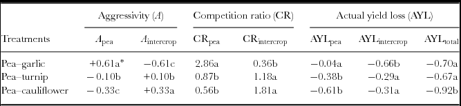
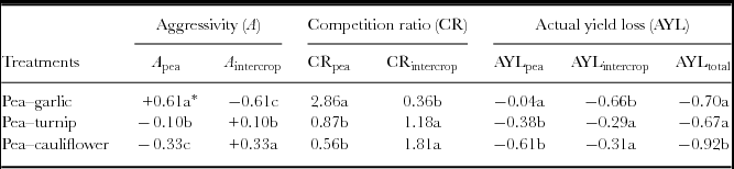
Data regarding aggressivity demonstrates that both component vegetables in each intercropping system did not compete equally. Positive sign of A pea value in the pea–garlic intercropping system indicates its dominant behaviour over garlic. However, for the pea–turnip and pea–cauliflower intercropping systems, A pea values were found negative (Table 3), indicating that pea was a dominated vegetable in these intercropping systems. However, A pea and A intercrop values for different intercropping systems were statistically different from each other.
Effect of pea based intercropping systems on aggressivity, competition ratio and actual yield loss of pea, garlic, turnip and cauliflower.
*Mean values sharing similar letter(s) in a column are statistically non-significant at p = 0.05 (LSD test).
Competition ratio value for pea (CRpea) was significantly higher in the pea–garlic intercropping than the pea–turnip and pea–cauliflower intercropping systems, indicating that pea was more competitive than garlic. However, CRintercrop values were significantly greater for cauliflower, followed by turnip than pea in the pea–cauliflower and pea–turnip intercropping systems, exhibiting competitiveness of cauliflower and turnip over pea (Table 3). However, these two values were statistically similar.
All the values for actual yield loss, i.e. for AYLpea, AYLintercrop and AYLtotal were negative, indicating yield loss of both crops in all the intercropping systems, although their magnitude was different. Maximum AYLpea and AYLtotal (−0.61 and −0.92 respectively) were observed in the case of pea–cauliflower intercropping system. However, the maximum value for AYLintercrop (−0.66) was found in the case of pea–garlic intercropping system, which was significantly different from other two values (Table 3), indicating maximum yield loss of garlic in the pea–garlic intercropping system.
Economic and monetary advantages
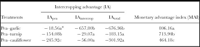
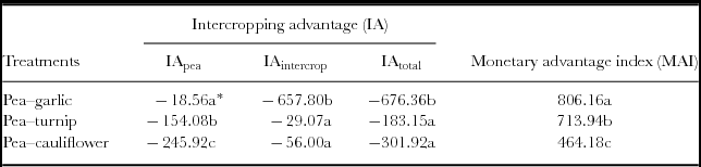
For all the intercropping systems, partial IA values for both pea and intercrops were negative. Thus, total IA values were also negative. Data showed that partial IA value for pea (−18.56) was significantly higher in case of pea–garlic intercropping as compared with other intercropping systems (−154.08 and −245.92). Partial IA values for intercrops were higher for turnip (−29.07) and cauliflower (−56.00) in the pea–turnip and pea–cauliflower intercropping systems as compared to garlic (−657.80) in the pea–garlic intercropping system. Former two values were statistically similar but were significantly different from the latter one. Total IA values affirmed that the pea–turnip intercropping system was comparatively less disadvantageous with the highest IA value of −183.15 followed by pea–cauliflower with the IA value of −301.92. These two intercropping systems behaved statistically similar for total IA value. The lowest total IA value of −676.36 indicated that the pea–garlic intercropping system led to the highest loss, which was significantly higher than other intercropping systems (Table 4). However, MAI values for all the cropping systems were positive, clearly indicating monetary advantage of intercropping. All the three values were statistically different from each other. The highest MAI value was recorded for the pea–garlic intercropping system, followed by the pea–turnip system, thus having better economic advantage. The pea–cauliflower intercropping system resulted in the lowest MAI value (Table 4).
Effect of pea based intercropping systems on intercropping advantage and monetary advantage index.
*Mean values sharing similar letter(s) in a column are statistically non-significant at p = 0.05 (LSD test).
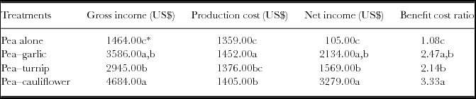
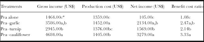
Economic analysis indicated that pea intercropping with cauliflower, turnip and garlic achieved higher net income and BCR as compared with pea alone. Among the intercropping systems, the pea–cauliflower intercropping outperformed with higher net income (US$ 3279) and BCR (3.33) (Table 5).
Economics of pea-based intercropping systems.
*Mean values sharing similar letter(s) in a column are statistically non-significant at p = 0.05 (LSD test).
Discussion
Crop yield and harvest index
Higher vegetable yields of monocropped pea, garlic, turnip and cauliflower as compared with intercropping treatments were probably due to no competition for soil nutrients, moisture, sunlight and other resources with some other crop and less disturbance in the habitat in homogeneous environment of monocropping system (Banik et al., Reference Banik, Midya, Sarkar and Ghose2006; Grime, Reference Grime1977; Qasim et al., Reference Qasim, Anjum, Ahmad and Hussain2013). Similar results have been reported by Hussain (Reference Hussain2003) when pea was tested in combination with cauliflower, potato, lettuce, reddish, turnip, coriander and spinach. In the pea–garlic intercropping system, the yield of pea was slightly affected but the yield of garlic was adversely affected. These both are shallow rooted vegetables and pea can exploit resources more efficiently than garlic. Roots of turnip and cauliflower can penetrate deeper than the pea and can absorb water and nutrients more efficiently; therefore, in the pea–turnip and pea–cauliflower intercropping systems, the yield of pea was more affected as compared with turnip and cauliflower. Further, this yield reduction in the intercropping systems was due to inter-plant competition between the intercrops for growth resources such as soil, water and nutrients. Hussain (Reference Hussain2003) found that yield of pea was adversely affected when intercropped with cauliflower, reddish or turnip. Similarly, pea yield was significantly decreased when intercropped with oat (Jannoura et al., Reference Jannoura, Joergensen and Bruns2014). Banik et al. (Reference Banik, Sasmal, Ghosal and Bagchi2000) also reported reduced yields of mustard–pea, mustard–lentil and mustard–gram intercropping systems over their sole cropping. Total grain yields were also lower in the pea–oat intercropping system than in pure stands (Neugschwandtner and Kaul, Reference Neugschwandtner and Kaul2014). Choosing of partner crops in intercropping systems plays a vital role, and factors such as rooting system, nutrient competition and shading must be considered (Ijoyah and Fanen, Reference Ijoyah and Fanen2012; Ijoyah and Jimba, Reference Ijoyah and Jimba2012; Jannoura et al., Reference Jannoura, Joergensen and Bruns2014). Moreover, turnip and cauliflower have large canopies with broad leaves, which intercepted light and casted shade on pea plants, creating a microclimate that resulted in reduced yield of pea in the pea–turnip and pea–cauliflower intercropping systems. Therefore, for obtaining higher yields in intercropping systems, competition among partner crops can be minimized by spatial arrangement and also by choosing right crops (Hadidi et al., Reference Hadidi, Sharaiha and Al-Debei2011; Ijoyah, Reference Ijoyah2012; Munz et al., Reference Munz, Graeff-Honninger and Lizaso2014).
Harvest index is an important parameter to assess effect of a specific treatment in allocating nutrients and carbohydrates in relative proportions of vegetative and reproductive parts (Hussain, Reference Hussain2003). Harvest indices of garlic, turnip and cauliflower were not affected when these were intercropped with pea. However, HI of pea was significantly decreased when intercropped with turnip and cauliflower. Turnip and cauliflower are broad-leaved vegetables, and in the intercropping systems these intercepted more radiation and casted shade on pea plants. This reduced photosynthetic activities in pea leaves, resulting in low economic yield and hence low HI. The HI of pea also decreased when intercropped with oat due to shading effect of oat during grain development (Neugschwandtner and Kaul, Reference Neugschwandtner and Kaul2014). Under stress conditions, alteration in allocation of resources is a part of strategy to avoid or overcome the stress condition. Under mild stress, reproductive growth is a common strategy. However, severe stress causes decrease in reproductive growth (Boraj et al., Reference Boraj, Singh and Kanar2001), as it happened in the present case with pea when intercropped with turnip and cauliflower.
Competition functions
The LER is the most common index used in intercropping for measuring land productivity. In intercropping, yield advantage occurs due to differences between component crops in using the growth resources. The LER is employed to evaluate the efficiency of intercropping for using the growth resources as compared with monocropping. Higher LERpea value in the pea–garlic intercropping system indicates better resource utilization of pea in this cropping system. Therefore, in this cropping system, there was an advantage for pea and disadvantage for garlic. However, higher LERintercrop values in the case of pea–cauliflower and pea–turnip intercropping systems were possibly due to better land and resources utilization by cauliflower and turnip in their respective intercropping system. This also indicates that in these intercropping systems, cauliflower and turnip have an advantage and pea has disadvantage. Hussain (Reference Hussain2003) also reported that cauliflower and turnip were uneconomic combinations of pea because of low value of LER. In all the intercropping systems, LERtotal values were more than 1, indicating over-yielding capacity of the intercropping systems over their sole crops due to better utilization of available resources for plant growth. Similar results have been reported for the pea–barley (Chen et al., Reference Chen, Westcott, Neill, Wichman and Knox2004) and pea–oat (Jannoura et al., Reference Jannoura, Joergensen and Bruns2014) intercropping systems.
Relative K value describes the dominance of component crops in intercropping systems. The crop with high K value is dominant over the crop with low K value. Aggressivity demonstrates competitive behaviour and aggressiveness of component crops in intercropping systems. A zero value of A indicates that the component crops in the intercropping system are equally competitive. Normally, both crops have the same numerical value but the sign may be positive or negative. The crop with positive A value is dominant crop and that with negative sign is dominated crop. Competition ratio (CR) is an important tool to measure the degree of competition between component crops in intercropping systems, and high CR value indicated higher competitive ability of crop. Actual yield loss (AYL) is based on crop yield and describes the proportionate yield loss or gain of each crop when grown as intercrop in comparison with its yield as monocrop. In the present study, K, A, CR and AYL values demonstrated the dominance of pea in the pea–garlic intercropping system, as garlic was more affected in the cropping system. However, cauliflower and turnip were dominant in the pea–cauliflower and pea–turnip intercropping systems respectively. In other words, turnip and cauliflower were more competitive and aggressive than pea, and pea was more competitive and aggressive than garlic. LERpea and Kpea values followed a similar trend. Further, LERintercrop and Kintercrop were also in line. In all the cropping systems, total K values were more than 1, indicating a definite yield advantage due to intercropping in terms of better use of land and other available resources for plant growth (Chen et al., Reference Chen, Westcott, Neill, Wichman and Knox2004). Intercropping advantage in terms of LER and K have already been reported in intercropping of pea or vetch with different cereals such as wheat, triticale, barley and oat (Bedoussac and Justes, Reference Bedoussac and Justes2010; Dhima et al., Reference Dhima, Lithourgidis, Vasilakoglou and Dordas2007). It is clear from the competition functions that the occurred advantage was due to better efficiency in the utilization of available growth resources such as water, nutrients and radiation energy by these vegetables in the respective intercropping systems.
The actual yield loss index can give more precise information than other indices about the intra-crop and inter-crop competition between component crops and behaviour of each crop in an intercropping system (Banik et al., Reference Banik, Sasmal, Ghosal and Bagchi2000). All AYL values were negative, indicating yield loss of both crops and disadvantage of intercropping. This was probably due to the fact that nitrogen fixing ability of pea could not compensate vigorous growth of other component vegetables over a certain proportion. There was 65.78% yield loss of garlic in garlic–pea intercropping and 61.48% yield loss of pea when intercropped with cauliflower compared with their sole crop yields. In the case of pea–garlic intercropping, AYLpea was greater than AYLintercrop, indicating that pea was more resistant to yield loss than garlic in this cropping system.
Economic and monetary advantages
In intercropping systems, economic value and net profit to the growers is also important (Dordas et al., Reference Dordas, Vlachostergios and Lithourgidis2012) as overall success and adoptability of any system depends upon its economic feasibility. The IA and MAI values are considered as indicators of economic feasibility of intercropping systems, and these show which intercrop is the most advantageous one (Banik et al., Reference Banik, Sasmal, Ghosal and Bagchi2000; Dordas et al., Reference Dordas, Vlachostergios and Lithourgidis2012). As AYL values were negative, IA values were also negative. As total AYL value was higher in the case of pea–turnip intercropping, it also resulted in high total IA value. Thus, the pea–turnip intercropping system was comparatively less disadvantageous, and the pea–garlic intercropping system resulted into the highest loss.
The MAI values also significantly differed for the studied intercropping systems, possibly due to differences in the values of intercrops, LER and other competition indices and also other factors like morphology, physiology and differential nutrients requirements of the vegetables used in the intercropping systems. In particular, different root size and depth of the vegetables also affected the utilization of available resources. The greatest MAI value (806.16) was recorded in the case of pea–garlic intercropping system, which implies the most advantageous intercropping system, indicating definite yield and economic advantages compared with sole cropping. MAI values for all the cropping systems were also in accordance with A, CR and K values. Ghosh (Reference Ghosh2004) also reported that when the K value was high, the MAI value was also high, indicating a significant economic advantage. According to the economic analysis, pea–cauliflower outperformed with higher net income and BCR as compared with other intercropping systems and pea alone. Although individual yields of both cauliflower and pea were reduced in intercropping system than their sole crops, higher relative yield of both the vegetables in the intercropping systems compensated it, which resulted in higher net income and BCR. According to Brintha and Seran (Reference Brintha and Seran2009), intercropping occupies greater land use and results in higher net return. Higher economic return from intercropping as compared with monocropping has already been reported for mustard–onion and mustard–garlic intercropping systems (Saker et al., Reference Saker, Rahman and Das2007).
Conclusions
Vegetable yields were higher when pea, garlic, turnip and cauliflower were grown alone. In intercropping, yields of all the vegetables decreased due to competition for available growth resources. However, pea was more competitive, aggressive and dominant having yield advantage in the pea–garlic intercropping, while in the case of pea–cauliflower and pea–turnip intercropping, cauliflower and turnip respectively had higher values of competition indices. High value of MAI for the pea–garlic intercropping system indicates that this was a more suitable intercropping system than the pea–turnip and pea–cauliflower intercropping systems. However, pea-cauliflower intercropping was the most profitable one with higher net income and BCR.