







1 Introduction
In this article, we mainly study the stability of the
 $L_p$
torsional measure, which is associated with the solution of
 $L_p$
-Minkowski problem for torsional rigidity. This study belongs to the
 $L_p$
-Brunn–Minkowski theory (see, e.g., [Reference Lutwak38, Reference Lutwak39, Reference Schneider46]).
To illustrate the
 $L_p$
torsional measure, let us first recall the classical Minkowski problem and its
 $L_p$
-generalized counterpart. The classical Minkowski problem asks what are the necessary and sufficient conditions of a Borel measure
 $\varphi $
such that
 $\varphi $
can be identified as the surface area measure of a convex body (compact convex set with nonempty interior). That is, find necessary and sufficient conditions of a Borel measure
 $\varphi $
on the sphere
 $S^{n-1}$
to guarantee that there exists a convex body K in
 $\mathbb {R}^n$
such that
 $$ \begin{align*}S(K,\cdot)=\varphi, \end{align*} $$
where the surface area measure
 $S(K,\cdot )$
is a Borel measure on the unit sphere
 $S^{n-1}$
defined as the push forward to
 $S^{n-1}$
of the
 $(n-1)$
-dimensional Hausdorff measure on
 $\partial K$
via the Gauss map
 $\mathcal {V}_K$
, and the Gauss map,
 $\mathcal {V}_K: \partial K\rightarrow S^{n-1}$
, maps every
 $x\in \partial K$
to the set of its unit normal vectors with respect to K. The classical Minkowski problem serves as the major force behind the Brunn–Minkowski theory. In particular, it plays a core ingredient in the Brunn–Minkowski type inequality and affine isoperimetric inequalities (see Schneider [Reference Schneider46] for more details).
In 1962, Firey [Reference Firey23] introduced the concept of the
 $L_p$
-sum of convex bodies, which is a pivotal step to extend the classical Brunn–Minkowski theory to the
 $L_p$
cases. After that, Lutwak [Reference Lutwak38] introduced the
 $L_p$
surface area measure and posed the
 $L_p$
-Minkowski problem, which asks the conditions of a given Borel measure
 $\varphi $
on
 $S^{n-1}$
such that there exists a convex body K in
 $\mathbb R^n$
such that
 $\varphi $
is the
 $L_p$
surface area measure of K. When
 $p=1$
, the
 $L_p$
-Minkowski problem reduces to the classical Minkowski problem. The
 $L_p$
-Minkowski problem has been a central object of interest in convex geometric analysis for the last decades and has received extensive considerations (see, e.g., [Reference Böröczky and Saroglou6, Reference Böröczky and Trinh7, Reference Chou and Wang13, Reference Fang, Xing and Ye19, Reference Hu, Ma and Shen26, Reference Hug, Lutwak, Yang and Zhang29, Reference Ivaki30, Reference Lu and Wang37, Reference Lutwak and Oliker40, Reference Lutwak, Yang and Zhang41, Reference Umanskiy50, Reference Zhu54]). There are various extensions of Minkowski problems, for instance, the logarithmic Minkowski problems (see, e.g., [Reference Böröczky, Hegedus and Zhu4, Reference Böröczky, Lutwak, Yang and Zhang5, Reference Zhu53] and the
 $L_p$
dual Minkowski problem and Orlicz–Minkowski problem (see, e.g., [Reference Ai, Yang and Ye1, Reference Fang, Ye, Zhang and Zhao20, Reference Haberl, Lutwak, Yang and Zhang25, Reference Li, Ye and Zhu35]).
The
 $L_p$
torsional measures are central concept in the
 $L_p$
-Minkowski problem for torsional rigidity. We now recall the definitions of torsional rigidity and
 $L_p$
torsional measures. Let K be a convex body with
 $C^2_+$
boundary, whose interior is denoted by
 $\Omega $
. The classical torsional rigidity can be expressed in the form of variation given by
 $$ \begin{align} \frac{1}{\tau(K)}=\inf\left\{\frac{\int_{\Omega}|\nabla v|^2\mathrm{d}x}{\left(\int_{\Omega}|v|\mathrm{d}x\right)^2}: v\in W_0^{1,2}, \int_{\Omega}|v|\mathrm{d}x>0\right\}. \end{align} $$
Note that the minimizer u in (1.1) is the unique solution of boundary value problem
 $$ \begin{align} \left\{\begin{array}{ll} \Delta u=-1 & \text { in } \Omega, \\ u=0 & \text { on } \partial \Omega, \end{array}\right. \end{align} $$
where
 $\Omega $
is the interior of convex body K, and
 $\Delta =\sum \limits _{i=1}^n \frac {\partial ^2}{\partial x_i^2}$
is the classical Laplace operator. Colesanti and Fimiani [Reference Colesanti and Fimiani16] defined the torsional measure
 $\mu ^{\mathrm{tor}}(K,\cdot )$
by
 $$ \begin{align*} \mu^{\mathrm{tor}}(K,E)=\int_{\mathcal{V}^{-1}_K(E)}|\nabla u|^{2} \mathrm{d}\mathcal{H}^{n-1}, \end{align*} $$
for Borel set
 $E\subset S^{n-1}$
, where u is the minimizer in the definition of
 $\tau (K)$
,
 $\mathcal {V}^{-1}_K$
is the inverse Gauss map of K, and
 $\mathcal {H}^{n-1}$
is the
 $(n-1)$
-dimensional Hausdorff measure. Using the definition of the torsional measure, Chen and Dai [Reference Chen and Dai12] introduced the
 $L_p$
torsional measure
 $\mu ^{\mathrm{tor}}_{p}(K, \cdot )$
as
 $$ \begin{align} \mu^{\mathrm{tor}}_{p}(K, E)=\int_{E}h_K(\xi)^{1-p}\mathrm{d}\mu^{\mathrm{tor}}(K, \xi), \end{align} $$
for Borel set
 $E\subset S^{n-1}$
, where
 $h_K(x)=\sup \{x\cdot y:y\in K\}$
is the support function of K, and
 $x\cdot y$
is the inner product in
 $\mathbb R^n$
. If we write
 $h=h_K$
for the brevity, the
 $L_p$
torsional measure can be written as
 $$ \begin{align} \mu_p^{\mathrm{tor}}(K,E)=\int_E h^{1-p}(\theta )|\nabla u(\mathcal{V}_K^{-1}(\theta))|^2\mathrm{det}(h_{ij}(\theta)+\delta_{ij}h(\theta))\mathrm{d}\theta \end{align} $$
for Borel set
 $E\subset S^{n-1}$
, where
 $\mathrm {d}\theta $
is the spherical Lebesgue measure on
 $S^{n-1}$
.
Suppose K is a convex body in
 $\mathbb {R}^n$
with
 $C^2_+$
boundary, and
 $\mu $
is a finite Borel measure on
 $S^{n-1}$
. The
 $L_p$
-Minkowski problem for torsional rigidity asks: what are the necessary and sufficient conditions such that
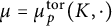 $\mu =\mu _p^{\mathrm{tor}}(K,\cdot )$
? In the case
 $p=2$
, the existence and uniqueness of the solution of the Minkowski problem for torsional rigidity was proved by Colesanti and Fimiani [Reference Colesanti and Fimiani16]. Under the assumption of existence, Sun, Xu, and Zhang [Reference Sun, Xu and Zhang49] proved the uniqueness of the
 $L_p$
-Minkowski problem for q-torsional rigidity for
 $p>1, q>1$
. Chen, Zhao, Wang, and Zhao [Reference Chen, Zhao, Wang and Zhao11] introduced the generalized
 $L_p q$
-torsional measure
 $p\in \mathbb {R}$
and
 $q>1$
, and considered the existence of the related
 $L_p$
-Minkowski type problem. See also [Reference Bu, Qin and Wu8] for some Minkowski type estimations about the generalized torsional rigidity. For
 $n\geq 3$
,
 $p>1$
, and
 $p\neq n+2$
, Chen and Dai [Reference Chen and Dai12] recently established the existence and uniqueness of the solution of the
 $L_p$
-Minkowski problem for torsional rigidity, which states that: for any fixed
 $n\geq 3,\;p>1$
, and
 ${p\neq n+2}$
, if
 $\mu $
is a positive and finite Borel measure on
 $S^{n-1}$
, which is not concentrated on any closed hemisphere, that is,
 $$ \begin{align*}\inf\limits_{e\in S^{n-1}}\int_{S^{n-1}}(e\cdot \theta)_+\mathrm{d}\mu(\theta)>0,\end{align*} $$
where
 $(e\cdot \theta )_+ = \max \{e\cdot \theta , 0\}$
, then there exists a unique convex body
 $\Omega \in \mathcal {K}_o^n$
such that
 $\mu _p^{\mathrm{tor}}(\Omega , \cdot )=\mu (\Omega , \cdot ).$
By (1.4), the
 $L_p$
torsional measure has the Radon–Nikodym derivative with respect to the spherical Lebesgue measure as
 $$ \begin{align} \frac{\mathrm{d}\mu_p^{\mathrm{tor}}(K,\xi)}{\mathrm{d}\xi}=|\nabla u|^2h_K^{1-p}f_K, \end{align} $$
where
 $f_K$
denotes the curvature function of convex body K, which is the reciprocal of the Gauss curvature in the sense of (2.1).
Motivated by the uniqueness and existence of the
 $L_p$
-Minkowski problem for torsional rigidity given in [Reference Chen and Dai12], our first main result answers the related overdetermined boundary value problem as follows.
Theorem 1.1 Let
 $n\geq 3$
,
 $p>1$
with
 $p\neq n+2$
, and let c be a positive constant. Assume there exists a solution
 $u\in C^2(\Omega )\cap C^1(\bar {\Omega })$
to the overdetermined boundary value problem
 $$ \begin{align*}\nonumber \left\{\begin{array}{@{}ll} \Delta u = -1 & \text{ in } \Omega,\\ u\equiv 0 & \text{ on } \partial\Omega, \quad u>0 \quad\text{ in } \Omega,\\ |\nabla u|^2h_\Omega^{1-p} = cG_\Omega & \text{ on }\partial\Omega, \end{array}\right. \end{align*} $$
where
 $G_\Omega $
is the Gauss curvature of the boundary
 $\partial \Omega $
. Then
 $\Omega $
must be a ball in
 $\mathbb {R}^n$
.
Theorem 1.1 combined with (1.5) implies that: for
 $n\geq 3$
and
 $p>1$
with
 $p\neq n+2$
, if
 $K\in \mathcal {F}_o^n$
satisfies
 $$ \begin{align*}|\nabla u|^2h_K^{1-p}f_K\equiv c,\end{align*} $$
where u is the minimizer in the definition of
 $\tau (K)$
, then K is a ball in
 $\mathbb {R}^n$
. It is natural to ask whether convex body
 $K\in \mathcal {F}_o^n$
is close to a ball in a suitable sense if
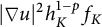 $|\nabla u|^2h_K^{1-p}f_K$
is not a constant but close to a constant in some sense?
In this article, we study whether there exists an increasing function f with
 $\lim _{\varepsilon \to 0}f(\varepsilon )=0$
such that
 $K\in \mathcal {F}_o^n$
is
 $f(\varepsilon )$
-close to a ball if K satisfies
 $\mathcal {R}_{p}(K)\leq 1+\varepsilon $
, where
 $\mathcal {R}_{p}(K)$
is defined by, for
 $K\in \mathcal {F}_o^n$
,
 $$ \begin{align*} \mathcal{R}_{p}(K)=\frac{\max\limits_{S^{n-1}}|\nabla u|^2h_K^{1-p}f_K}{\min\limits_{S^{n-1}}|\nabla u|^2h_K^{1-p}f_K}. \end{align*} $$
Note that
 $\mathcal {R}_p(tK)=\mathcal {R}(K)$
for
 $t>0$
. This follows from the homogeneity of support function and curvature function and a fact that
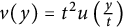 $v(y)=t^2u\left (\frac {y}{t}\right )$
is the solution of (1.2) in
 $t\Omega $
when
 $u(x)$
satisfies (1.2) in
 $\Omega $
(see [Reference Huang, Song and Xu28] for more details).
To address the aforementioned question, we first need to define what “close” means. In this article, we utilize the concepts of the relative asymmetry distance and the
 $L^c$
-distance (
 $c\geq 2$
), respectively, to measure how “close” two convex bodies are.
The relative asymmetry is defined by using the volume symmetric difference of two bodies with the same volume. The relative asymmetry
 $\mathcal {A}(K,L)$
between
 $K, L\in \mathcal {K}^n$
is defined by
 $$ \begin{align*} \mathcal{A}(K,L)=\inf\limits_{x\in\mathbb{R}^n}\frac{V(K\Delta(\lambda L+x))}{V(K)}, \end{align*} $$
where
 $\lambda ^n=\frac {V(K)}{V(L)}$
and
 $K\Delta L=(K\backslash L)\cup (L\backslash K)$
denotes the symmetric difference between convex bodies
 $K, L\in \mathbb {R}^n$
.
In the sequel, we denote by
 $\tilde {K}$
the dilation
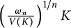 $\left (\frac {\omega _n}{V(K)}\right )^{1/n}K$
, which has the same volume as the unit ball in
 $\mathbb {R}^n$
. Using the relative asymmetry distance, we have the following global stability result of the
 $L_p$
torsional measure.
Theorem 1.2 Suppose
 $n\geq 3$
,
 $p> 1$
, and
 $p\neq n+2$
. Then there exists a constant C independent of the dimension, such that any
 $K\in \mathcal {F}_o^n$
satisfies
 $$ \begin{align*}\mathcal{A}(\tilde{K},B_2^n)^2\leq Cn^5\left(c_{n,K}\mathcal{R}_{p}(K)^{\frac{1}{p}}-1\right),\end{align*} $$
where
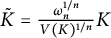 $\tilde K=\frac {\omega _n^{1/n}}{V(K)^{1/n}}K$
,
 $c_{n,K}=\frac {w(\tilde K)}{2}$
,
 $\omega (K)=\frac {2}{n\omega _n}\int _{S^{n-1}}h_{K}(u)\mathrm {d}u$
is the mean width of K, and
 $\omega _i$
is the volume of the i-dimensional ball.
To complete the proof of Theorem 1.2, we utilize not only the
 $L_p$
-Minkowski inequality for torsional rigidity (3.15) but also the refined Urysohn’s inequality (2.3) and the Urysohn type inequality for torsional rigidity (3.12). Note that it holds
 ${c_{n,K}=\frac {w(\tilde K)}{2} =\frac {\omega _n^{1/n}}{V(K)^{1/n}} \frac {w(K)}{2} \geq 1}$
by Urysohn’s inequality (2.2), and the equality holds when K is a ball.
In Theorems 1.3 and 1.4, we use a different distance to derive the stability problem of the
 $L_p$
torsional measure for the dimension
 $n\geq 3$
, namely utilizing the
 $L^c$
-distance to give the related local and global stability results for the cases
 $p\in (1,n)$
, and
 $p>n$
with
 $p\neq n+2$
, respectively. The
 $L^c$
-distance of
 $K, L\in \mathcal {K}^n$
is defined by
 $$ \begin{align*} \delta_c(K,L)=\left(\frac{1}{n\omega_n}\int_{S^{n-1}}|h_K-h_L|^c\mathrm{d}u\right)^{\frac{1}{c}} \text{ for } c\geq 2. \end{align*} $$
In particular, let
 $c=2$
, then the
 $L^2$
-distance is defined by
 $$ \begin{align*} \delta_2(K,L)=\left(\frac{1}{n\omega_n}\int_{S^{n-1}}|h_K-h_L|^2\mathrm{d}u\right)^{\frac{1}{2}}. \end{align*} $$
The result states as follows.
Theorem 1.3 Suppose
 $n\geq 3$
and
 $p\in (1,n)$
. Let
 $K\in \mathcal {F}_o^n$
with
 $e_p(K)=0$
(see Definition 4.1 and its remark for the definition of
 $e_p(K)$
), and assume
 $|h_{\lambda K}-1|_{C^3}\leq \delta $
for some
 $\delta , \lambda>0$
. Suppose further that
 $B_2^n(r_0)\subset \tilde {K}$
for some
 $0<r_0\leq 1$
. Then there exist
 $\gamma _1$
depending on p and n, and a universal constant
 $\gamma _2>0$
such that
 $$ \begin{align*}\delta_{c_1}(\tilde{K}, B_2^n)^2\leq \gamma_1\left(1-c_{n,K}^{-p}\left(1-\gamma_2\left(\mathcal{R}_{p}(K)-1\right)^2\right)\right),\end{align*} $$
where
 $c_1=\max \left \{\frac {n}{n-p},\frac {n}{p}\right \}\geq 2$
and
 $c_{n, K}=\frac {\omega (\tilde {K})}{2}$
.
Theorem 1.3 provides the local stability of
 $L_p$
torsional measure for
 $1<p<n$
, for which the proof is mainly based on the Łojasiewcz inequality [Reference Simon48] and the stability of Hölder’s inequality (5.2). In the case
 $p>n$
with
 $p\neq n+2$
, we give in Theorem 1.4 a global stability result by using stability of reverse Hölder’s inequality [Reference Aldaz2].
Theorem 1.4 Let
 $n\geq 3$
,
 $p>n$
, and
 $p\neq n+2$
. Suppose
 $K\in \mathcal {F}_o^n$
satisfies
 $e_p(K)=0$
and
 $\tilde {K}$
contains a ball
 $B_2^n(r_0)$
for some
 $0<r_0\leq 1$
. Then there exists an origin-centered ball
 $B_2^n(r)$
with radius r satisfying
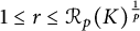 $1\leq r\leq \mathcal {R}_{p}(K)^{\frac {1}{p}}$
, and a constant
 $\gamma $
depending on
 $r_0, p, n$
, and the diameter
 $D(K)$
, such that
 $$ \begin{align*}\delta_2(\tilde{K},B^n_2(r))^2\leq \gamma c_{n,K}^{2p}\mathcal{R}_{p}(K)^2 \left(1-c_{n,K}^{-n}\mathcal{R}_{p}(K)^{-\frac{n}{p}}\right).\end{align*} $$
Here,
 $c_{n,K}=\frac {\omega (\tilde {K})}{2}$
. In particular, if p is an integer, then the constant
 $\gamma $
only depends on n and
 $D(K)$
.
Notice that the constant
 $c_{n,K}=\frac {\omega (\tilde {K})}{2}=\frac {\omega _n^{1/n}}{V(K)^{1/n}}\frac {w(K)}{2}$
appears in Theorems 1.2–1.4. This is due to the fact that our proofs crucially rely on the Urysohn type inequality for torsional rigidity (3.12).
The article is organized as follows. Some definitions and inequalities related to convex bodies are introduced in Section 2. Section 3 begins by reviewing fundamental concepts of torsional rigidity, then presents a concise proof of the Urysohn type inequality for q-torsional rigidity in Theorem 3.2, which serves as a key tool in establishing Theorems 1.2 and 1.3. Additionally, we complete the proof of Theorem 1.1 at the end of Section 3. In Sections 4– 6, we derive stability estimates for the
 $L_p$
-widths, as presented in Lemma 4.2 and Theorems 5.3 and 6.2. Based on these results, we subsequently establish all related global and local stability conclusions of this article, employing the relative asymmetry distance and the
 $L^c$
-distance, respectively.
2 Preliminary
In this section, we recall some basic concepts of convex bodies. The reader can refer to the excellent books [Reference Gardner24, Reference Schneider46] for more information.
We work with the Euclidean space
 $\mathbb {R}^n$
. Let
 $\mathcal {K}^n$
be the class of convex bodies (compact convex sets with nonempty interior) in
 $\mathbb {R}^n$
, and
 $\mathcal {K}_o^n$
be the class of convex bodies containing the origin in the interiors. Moreover,
 $\mathcal {F}^n$
and
 $\mathcal {F}_o^n$
represent the set of smooth, strictly convex bodies in
 $\mathcal {K}^n$
and
 $\mathcal {K}_o^n$
, respectively. We write
 $B_2^n$
for the Euclidean unit ball in
 $\mathbb {R}^n$
and
 $S^{n-1}$
for the sphere of
 $B_2^n$
, throughout the article. For a convex body K in
 $\mathbb {R}^n$
, we write
 $V(K)$
to stand for the volume of K. Specially, the volume of
 $B_2^n$
is
 $V(B_2^n)=\frac {1}{n}\int _{S^{n-1}}\mathrm {d}\sigma =\omega _n$
. The body
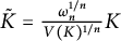 $\tilde {K}=\frac {\omega _n^{1/n}}{V(K)^{1/n}}K$
is the dilation of K such that
 $V(\tilde {K})=\omega _n$
.
For a convex body K in
 $\mathbb {R}^n$
, its support function
 $h_K$
is defined by, for
 $y\in \mathbb {R}^n$
,
 $$ \begin{align*} h_K(y)=\sup\limits_{x\in K}\{x\cdot y\}, \end{align*} $$
where
 $x\cdot y$
is the standard inner product in
 $\mathbb {R}^n$
. Note that the support function
 $h_K$
is continuous and homogeneous of degree
 $1$
. A convex body is uniquely determined by its support function.
If
 $K\in \mathcal {F}_o^n$
, the Gauss map
 $\mathcal {V}_K: \partial K\to S^{n-1}$
is a map taking
 $x\in \partial K$
to its unique outer unit normal vector. Here,
 $\partial K$
denotes the boundary of K. Denote that
 $$ \begin{align*}\mathcal{V}_K^{-1}: S^{n-1} \to \mathbb{R}^n\end{align*} $$
is the inverse Gauss map of
 $\partial K$
. Associated with Gauss curvature
 $G_K$
, the curvature function
 $f_K$
is defined by
 $$ \begin{align} f_K=\frac{1}{G_K\circ\mathcal{V}_K^{-1}}. \end{align} $$
And the function
 $h_K^{1-p}f_K$
is called the
 $L_p$
-curvature function of K.
The class of convex bodies in
 $\mathbb {R}^n$
is the fundamental object in the classical Brunn–Minkowski theory. It combining with the Minkowski sum derives the concept of the mixed volume, which relates to the Minkowski inequality and Minkowski problems.
For
 $K,L\subseteq \mathbb {R}^{n}$
, and
 $\lambda \in (0,1)$
, the Minkowski sum
 $\lambda K+(1-\lambda ) L$
is given by
 $$ \begin{align*}\lambda K+(1-\lambda) L=\{\lambda x+(1-\lambda) y: x\in K,y\in L\}.\end{align*} $$
From the Minkowski sum, it leads to the mixed volume
 $V_1(K,L)$
of
 $K, L\in \mathcal {K}^n$
defined by
 $$ \begin{align*} V_1(K,L)=\frac{1}{n}\lim\limits_{\varepsilon\rightarrow 0}\frac{V(K+\varepsilon L)-V(K)}{\varepsilon}. \end{align*} $$
The surface area measure
 $S(K,\cdot )$
provides the following integral representation for
 $V_1(K,L)$
:
 $$ \begin{align*} V_1(K,L)=\frac{1}{n}\int_{S^{n-1}}h_L(u)\mathrm{d}S(K, u), \end{align*} $$
where
 $L\in \mathcal {K}^n$
.
Let
 $p\geq 1$
, and
 $K, L\in \mathcal {K}_o^n$
. Firey [Reference Firey23] defined the
 $L_p$
linear combination
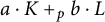 $a\cdot K+_p b\cdot L$
whose support function is given by
 $$ \begin{align*}h_{a\cdot K+_p b\cdot L}=(ah_K^p+bh_L^p)^{\frac{1}{p}}.\end{align*} $$
The symbol
 $+_p$
denotes the
 $L_p$
-sum (also called Firey sum). In particular, the
 $L_p$
-sum is just the classical Minkowski sum when
 $p=1$
. Motivated by the definition of
 $V_1(K,L)$
, Lutwak [Reference Lutwak38] defined the
 $L_p$
mixed volume
 $V_p(K,L)$
by using the
 $L_p$
-sum as
 $$ \begin{align*}\nonumber V_p(K,L)=\frac{p}{n}\lim\limits_{\varepsilon\rightarrow 0}\frac{V(K+_p \varepsilon\cdot L)-V(K)}{\varepsilon}. \end{align*} $$
In the case
 $p=1$
, the
 $L_p$
mixed volume
 $V_p(K,L)$
is the mixed volume
 $V_1(K,L)$
. The Brunn–Minkowski inequality, Minkowski inequality and their
 $L_p$
versions play central roles in the Brunn–Minkowski theory (see [Reference Bu and Wu9, Reference Lutwak38, Reference Lutwak39, Reference Schneider46, Reference Wu, Wang and Bu51, Reference Wu and Zhou52] for some extensions and applications).
In [Reference Lutwak38], Lutwak proved the significant variational formula of
 $V_p(K,L)$
for
 $p\geq 1$
that there exists a unique Borel measure
 $S_p(K, \cdot )$
on
 $S^{n-1}$
, named by
 $L_p$
surface area measure, such that
 $$ \begin{align*}\nonumber V_p(K,L)=\frac{1}{n}\int_{S^{n-1}}h_L^p(u)\mathrm{d}S_p(K, u). \end{align*} $$
Moreover, the
 $L_p$
surface area measure
 $S_p(K, \cdot )$
is absolutely continuous with respect to the surface area measure
 $S(K, \cdot )$
, and the Radon–Nikodym derivative is
 $$ \begin{align*}\frac{\mathrm{d} S_p(K, \cdot)}{\mathrm{d}S(K, \cdot)}=h_K^{1-p}(\cdot).\end{align*} $$
The generalized mixed volume for multiple convex bodies can be given by the following Steiner formula [Reference Schneider46], for any convex bodies
 $K_1, K_2, \ldots , K_m$
(
 $m\in \mathbb N$
),
 $$ \begin{align*}V(t_1K_1+\cdots+t_mK_m)=\sum\limits_{i_1,\ldots,i_n=1}^m t_{i_1}\ldots t_{i_n}V(K_{i_1},\ldots, K_{i_n}),\end{align*} $$
for any nonnegative numbers
 $t_1, t_2, \ldots , t_m$
. The coefficients
 $V(K_{i_1},\ldots , K_{i_n})$
are called the mixed volumes of
 $K_{i_1},\ldots , K_{i_n}$
.
The mixed volume
 $V(K_1, K_2, \ldots , K_n)$
is symmetric and multilinear, that is, for any permutation
 $\sigma $
of set
 $\{1, 2, \ldots n\}$
,
 $$ \begin{align*}V(K_1, K_2, \ldots, K_n)=V\left(K_{\sigma(1)}, K_{\sigma(2)}, \ldots, K_{\sigma(n)}\right);\end{align*} $$
and for any
 $\lambda , \mu \geq 0$
,
 $$ \begin{align*}V(\lambda K+\mu L, K_2, \ldots, K_n)=\lambda V(K, K_2, \ldots, K_n)+\mu V(L, K_2, \ldots, K_n).\end{align*} $$
For
 $K\in \mathcal K^n$
and
 $i=0,1,\ldots ,n$
, we call
 $$ \begin{align*}W_i(K)= V(K[n-i],B[i])\end{align*} $$
the i-th quermassintegral of K, where we use notation
 $A[m]$
for a convex set A repeated m times for the sake of brevity. We shall use
 $G(n,k)$
to denote the Grassmann manifold of k-dimensional subspaces of
 $\mathbb R^n$
, and
 $\mu _k$
to denote the usual normalized Haar measure on
 $G(n, k)$
, with
 $\mu _k(G(n,k)) = 1$
. Note that the i-th quermassintegral of K is proportional to the mean of the i-dimensional volumes of the projections of K onto the i-dimensional subspaces of
 $\mathbb R^n$
. Specifically,
 $W_0(K)=V(K)$
,
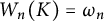 $W_n(K)=\omega _n$
. While for integer
 $0<i<n$
,
 $$ \begin{align*} W_i(K)= \frac{\omega_n}{\omega_{n-i}}\int_{G_{n,n-i}}V_{n-i}(K|\xi)\mathrm{d}\mu_{n-i}(\xi). \end{align*} $$
In particular,
 $(2/\omega _n)W_{n-1}(K)$
is the mean width of K. For
 $K\in \mathcal K^n_o$
, the width of K in some direction
 $u\in S^{n-1}$
is given by
 $h_K(u)+h_K(-u)$
, and the mean width
 $\omega (K)$
of K can also be written as
 $$\begin{align*}\omega(K)=\frac{2}{n\omega_n}\int_{S^{n-1}}h_K(u)\mathrm{d}u.\end{align*}$$
The Urysohn’s inequality gives the lower bound of
 $\omega (K)$
as
 $$ \begin{align} \frac{1}{2}\omega(K)\geq\left(\frac{V(K)}{V(B_2^n)}\right)^{\frac{1}{n}}, \end{align} $$
where equality holds if and only if K is a ball. Furthermore, as a consequence of the stability of the Brunn–Minkowski inequality due to Figalli, Maggi, Pratelli, and Segal [Reference Figalli, Maggi and Pratelli21, Reference Figalli, Maggi and Pratelli22, Reference Segal47], Segal [Reference Segal47] gave a refined Urysohn’s inequality about the relative asymmetry. It states that
Lemma 2.1 [Reference Segal47]
Let
 $K\in \mathcal K^n_o$
. We have
 $$ \begin{align} \frac{1}{n\omega_n}\int_{S^{n-1}}h_K(u)\mathrm{d}u\geq \left(\frac{V(K)}{V(B^n_2)}\right)^{\frac{1}{n}} \left(1+\left(\frac{\mathcal{A}(K,B^n_2)}{Cn^{2.5}}\right)^{2}\right). \end{align} $$
3 The variational formula of torsional rigidity and the uniqueness of torsional measure
In this section, we recall some fundamental concepts related to the torsional rigidity and study the uniqueness of the torsional measure.
For
 $q>1$
, suppose K is a convex body and its boundary is of class
 $C^2$
. Let
 $\Omega $
be the interior of convex body K. We define the q-torsional rigidity of K,
 $\tau _q(K)$
, by the following formula given in [Reference Colesanti, Cuoghi and Salani15]:
 $$ \begin{align} \frac{1}{\tau_q(K)}=\inf\left\{\frac{\int_{\Omega}|\nabla v|^q\mathrm{d}x}{\left(\int_{\Omega}|v|\mathrm{d}x\right)^q}: v\in W_0^{1,q}, \int_{\Omega}|v|\mathrm{d}x>0\right\}. \end{align} $$
The q-torsional rigidity is homogeneous of degree
 $\alpha _0=n(q-1)+q$
, that is,
 $$ \begin{align*}\nonumber \tau_q(s K)=s^{\alpha_0}\tau_q(K)\quad \text{for every}~ s>0. \end{align*} $$
The above functional (3.1) admits a minimizer
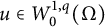 $u\in W_{0}^{1, q}(\Omega )$
, and
 $cu$
(for some constant c) is the unique positive solution of the following boundary value problem (see [Reference Belloni and Kawohl3] or [Reference Hu and Zhou27])
 $$ \begin{align} \left\{\begin{array}{@{}ll} \Delta_{q}u=-1 & \text { in } \Omega, \\ u=0 & \text { on } \partial \Omega , \end{array}\right. \end{align} $$
where
 $\Delta _{q}$
is the q-Laplace operator and
 $\Delta _{q}u=\mathrm {div}(|\nabla u|^{q-2}\nabla u)$
.
Applying the Gauss–Green formula with (3.2), we obtain
 $$ \begin{align*} \int_{\Omega}|\nabla u|^{q} \mathrm{d}x = \int_{\Omega} u(x) \mathrm{d}x. \end{align*} $$
Combining this with (3.1), we find the relation
 $$ \begin{align} \tau_q(K)=\left[\int_{\Omega} u(x) \mathrm{d}x\right]^{q-1}, \end{align} $$
where
 $u\in W_0^{1,q}$
stands for the minimizer that the functional (3.1) admits.
In particular, when
 $q=2$
, Formula (3.1) yields the definition of the torsional rigidity [Reference Pólya and Szegö42]. Namely, the torsional rigidity of K, denoted by
 $\tau (K)$
, is defined by
 $$ \begin{align} \frac{1}{\tau(K)}=\inf\left\{\frac{\int_{\Omega}|\nabla v|^2\mathrm{d}x}{\left(\int_{\Omega}|v|\mathrm{d}x\right)^2}: v\in W_0^{1,2}, \int_{\Omega}|v|\mathrm{d}x>0\right\}. \end{align} $$
Note that the minimizer
 $u\in W_0^{1,2}$
of torsional rigidity (3.4) is characterized as the unique solution to the following boundary value problem
 $$ \begin{align} \left\{\begin{array}{@{}ll} \Delta u=-1 & \text { in } \Omega, \\ u=0 & \text { on } \partial \Omega, \end{array}\right. \end{align} $$
where
 $\Delta $
is the classical Laplace operator. Clearly, the torsional rigidity
 $\tau (\cdot )$
is homogeneous of degree
 $n+2$
.
The Brunn–Minkowski inequality for the q-torsional rigidity states in [Reference Colesanti, Cuoghi and Salani15] that: for
 $K,L\in \mathcal K^n$
,
 $p>1$
, and
 $t\in [0,1]$
,
 $$ \begin{align} \tau_q((1-t)K+tL)^{\frac{1}{q+n(q-1)}}\geq (1-t)\tau_q(K)^{\frac{1}{q+n(q-1)}} +t\tau_q(L)^{\frac{1}{q+n(q-1)}}, \end{align} $$
with equality if and only if K is homothetic to L.
Let K and L be two convex domains of class
 $C^2_+$
. Specifically, the boundaries of the convex domains K and L are of class
 $C^2$
and admit positive Gauss curvature. We can obtain the Hadamard variational formula of torsional rigidity [Reference Huang, Song and Xu28] as follows:
 $$ \begin{align} \left.\frac{\mathrm{d}}{\mathrm{d} t} \tau\left(K+t L\right)\right|_{t=0}= \int_{\partial K} h_{L}(\mathcal{V}_K(\theta))|\nabla u(\theta)|^{2} \mathrm{d} \theta, \end{align} $$
where u is a minimizer which (3.4) admits, and
 $\mathcal {V}_K$
is the Gauss map. Motivated by the above variational formulation, the torsional measure
 $\mu ^{\mathrm{tor}}(K,\cdot )$
can be defined as
 $$ \begin{align} \mu^{\mathrm{tor}}(K,E)=\int_{\mathcal{V}_K^{-1}(E)}|\nabla u|^{2} \mathrm{d}\mathcal{H}^{n-1}=\int_{E}|\nabla u(\mathcal{V}_K^{-1}(\theta))|^{2} \mathrm{d}S(K,\theta) \end{align} $$
for Borel set
 $E\subset S^{n-1}$
. Here,
 $\mathcal {H}^{n-1}$
is the
 $(n-1)$
-dimensional Hausdorff measure. We observe that
 $$ \begin{align*}\nonumber \mu^{\mathrm{tor}}(sK,E)=s^{n+1}\mu^{\mathrm{tor}}(K,E). \end{align*} $$
Thus, using the definition of the torsional measure
 $\mu ^{\mathrm{tor}}(K,\cdot )$
, the
 $L_p$
torsional measure
 $\mu _p^{\mathrm{tor}}(K, \cdot )$
is defined by
 $$ \begin{align*}\nonumber \mu_p^{\mathrm{tor}}(K, E)=\int_{E}h_K(\xi)^{1-p}\mathrm{d}\mu^{\mathrm{tor}}(K, \xi),\quad E\subseteq S^{n-1}. \end{align*} $$
From (3.7), we define the mixed torsional rigidity by
 $$ \begin{align*} \tau(K,L)= \left.\frac{1}{n+2}\frac{\mathrm{d} \tau\left(K+t L\right)}{\mathrm{d} t} \right|_{t=0}=\frac{1}{n+2} \int_{\partial K} h_{L}(\mathcal{V}_K(\theta))|\nabla u(\theta)|^{2} \mathrm{d} \theta. \end{align*} $$
In particular, combining the relation
 $\tau (K,K)=\tau (K)$
with (3.8), we have
 $$ \begin{align*} \tau(K)=\frac{1}{n+2} \int_{S^{n-1}} h_{K}(\theta) \mathrm{d}\mu^{\mathrm{tor}}(K,\theta). \end{align*} $$
We next present a new proof of the Urysohn type inequality for q-torsional rigidity, from which we immediately have Urysohn type inequality for the classical torsional rigidity.
Now we recall some basic notions to be used subsequently (see [Reference Caffarelli and Cabré10, Reference Crandall, Ishii and Lions17, Reference Jia, Bao and Bo31–Reference Koike34, Reference Liu, Bu and Zhang36, Reference Salani45] for more details). The continuous operator
 $F(x,t,\xi ,A):\mathbb {R}^n\times \mathbb {R}\times \mathbb {R}^n \times S_n \to \mathbb {R}$
is said to be proper if it satisfies
 $$ \begin{align*}F(x,t_1,\xi,A)\leq F(x,t_2,\xi,A)\;\;\text{ whenever }t_1\geq t_2,\end{align*} $$
where
 $S_n$
is the set of the
 $n \times n$
real symmetric matrices. Let
 $\Gamma \subset S_n$
be a convex cone with vertex at the origin such that
 $\Gamma $
contains the cone of nonnegative definite symmetric matrices
 $S_n^+$
. We say that F is degenerate elliptic in
 $\Gamma $
if
 $$ \begin{align*}F(x,t,\xi,A_1)\leq F(x,t,\xi,A_2)\;\;\text{ whenever }A_1\geq A_2,\; A_1, A_2\in \Gamma.\end{align*} $$
Let u and
 $\phi $
be two functions defined on an open set
 $\Omega $
. We say that
 $\phi $
touches u from above at a point
 $x_0\in \Omega $
if
 $$ \begin{align*}\phi(x_0)=u(x_0)\quad \text{and}\quad \phi(x)\geq u(x)\quad\text{ for all } x \text{ in a neighborhood of } x_0.\end{align*} $$
An upper semicontinuous function u is called a viscosity subsolution of the equation
 $F=0$
in
 $\Omega $
if for every
 $C^2$
function
 $\phi $
that touches u from above at any point
 $x\in \Omega $
, it holds
 $$ \begin{align*}F(x, u(x), D\phi (x), D^2\phi(x))\geq 0.\end{align*} $$
Consider the following Dirichlet problem:
 $$ \begin{align} \left\{\begin{array}{@{}ll} F\left(x, u, D u, D^{2} u\right)=0 & \text { in } \Omega, \\ u=0 & \text { on } \partial \Omega, \\ u>0 & \text { in } \Omega, \end{array}\right. \end{align} $$
where
 $F(x,t,\xi ,A):\mathbb {R}^n\times \mathbb {R}\times \mathbb {R}^n \times S_n \to \mathbb {R}$
is a continuous proper elliptic operator. Here,
 $Du$
and
 $D^{2}u$
are the gradient and the Hessian matrix of the function u, respectively.
Given an operator F, real number
 $\beta \in \mathbb {R}^+$
and vector
 $\theta \in \mathbb {R}^n$
, we set
 $$ \begin{align*} G_{\beta}^{(\theta)}(x, t, A)=F\left(x, t^{\frac{1}{\beta}}, t^{\frac{1}{\beta}-1} \theta, t^{\frac{1}{\beta}-3} A\right), \quad(x, t, A) \in \mathbb{R}^{n} \times(0, \infty) \times S_{n}. \end{align*} $$
We say that the operator F satisfies the comparison principle (CP) if the following statement holds:
(CP) Let
 $u\in C(\bar {\Omega })\cap C^2(\Omega )$
and
 $u^\prime \in C(\bar {\Omega })$
be a classical supersolution and a viscosity subsolution of
 $F=0$
such that
 $u\geq u^\prime $
on
 $\partial \Omega $
. Then
 $u\geq u^\prime $
in
 $\Omega $
.
By [Reference Salani45, Theorem 6.4] and [Reference Salani45, (7)], we have the following lemma, which is the key element in the proof of Theorem 3.2.
Lemma 3.1 Let
 $\Omega \in \mathbb {R}^n$
be a bounded open convex set,
 $\Omega ^{\sharp }$
be a ball having the same mean width as
 $\Omega $
, and
 $u,u^{\sharp }$
are the classical solutions of (3.9) in
 $\Omega ,\Omega ^{\sharp }$
, respectively, where F is a rotationally invariant proper elliptic operator satisfying the CP. For
 ${\beta \in (0,1)}$
, assume that the following set
 $$ \begin{align} \left\{(x,t,A)\in \mathbb{R}^n\times [0,+\infty)\times S_n:G_{\beta}^{(\theta)}(x, t, A)\geq 0 \right\} \end{align} $$
is convex, and assume furthermore that it holds
 $$ \begin{align} \liminf_{y \to x} \frac{\partial u(y)}{\partial \nu }>0 \quad \text{and}\quad \liminf_{y \to x} \frac{\partial u^{\sharp}(y)}{\partial \nu }>0 \end{align} $$
for every
 $x\in \partial \Omega , \partial \Omega ^{\sharp }$
, where
 $\nu $
is any inward direction of
 $\Omega ,\Omega ^{\sharp }$
at x. Then we have
 $$ \begin{align*}\nonumber \left \| u \right \| _{L^a(\Omega)}\leq \| u^{\sharp}\| _{L^a(\Omega^{\sharp})} \quad\text{for every} \quad a\in (0,+\infty]. \end{align*} $$
As an application of Lemma 3.1, we give in Theorem 3.2 the Urysohn type inequality for the q-torsional rigidity with
 $q>1$
.
Theorem 3.2 For
 $q>1$
, let
 $\Omega \in \mathbb {R}^n$
be an open bounded convex set and
 $\Omega ^\sharp $
be a ball with the same mean width as
 $\Omega $
. Then it holds
 $$ \begin{align*}\nonumber \tau_q(\Omega)\leq \tau_q(\Omega^\sharp), \end{align*} $$
with equality if and only if
 $\Omega =\Omega ^\sharp $
.
In particular, let
 $q=2$
, then
 $$ \begin{align} \tau(\Omega)\leq \tau(\Omega^\sharp), \end{align} $$
with equality if and only if
 $\Omega =\Omega ^\sharp $
.
Proof By a glance of (3.3) and Lemma 3.1, we just need to check that the q-Laplace operator satisfies all the conditions of Lemma 3.1. It is well known that q-Laplace operator satisfies the CP (refer to [Reference Pucci and Serrin43]) and it is obvious that q-Laplace operator is rotationally invariant. Since
 $\Omega $
is convex, we obtain that (3.11) holds due to [Reference Sakaguchi44].
We now show that the set (3.10) is convex for the Dirichlet problem (3.2). In fact, we may consider the following general Dirichlet type problem:
 $$ \begin{align*}\nonumber \left\{\begin{array}{@{}ll} \mathrm{div}(|\nabla u|^{q-2}\nabla u)+f(|x|,u,|Du|)=0 & \text { in } \Omega, \\ u=0 & \text { on } \partial \Omega, \\ u>0 & \text { in } \Omega. \end{array}\right. \end{align*} $$
If the function
 $$ \begin{align*}g^r_q(s,t)=t^{q+1-\frac{q-1}{\beta}}f(s,t^{\frac{1}{\beta}},t^{\frac{1}{\beta}-1}r)\end{align*} $$
is concave with respect to
 $(s,t)\in [0,\infty )\times [0,\infty )$
for every
 $r\geq 0$
and some
 $\beta \in (0,1)$
, then the set (3.10) is convex. In the case of (3.2),
 $f\equiv 1$
and we set
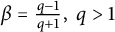 $\beta =\frac {q-1}{q+1},\;q>1$
, the function
 $g^r_q(s,t)\equiv 1$
satisfies the above properties. Thus, we obtain that
 $$ \begin{align*}\nonumber \left \| u \right \| _{L^1(\Omega)} \leq\| u^{\sharp}\| _{L^1(\Omega^{\sharp})}. \end{align*} $$
Then, from (3.3), we get
 $$ \begin{align*} \tau_q(\Omega)\leq \tau_q(\Omega^\sharp). \end{align*} $$
To establish the equality condition, we provide an alternative proof. Since
 $\tau _q$
is invariant under translations (see, e.g., [Reference Sun, Xu and Zhang49]), we may assume that the Steiner point of
 $\Omega $
coincides with the origin. Using Hadwiger’s theorem (see, e.g., [Reference Schneider46]), there exists a sequence of rotations
 $\{\rho _k\}$
such that
 $$ \begin{align*}\Omega_k=\frac{1}{k}(\rho_1\Omega+\cdots+\rho_k\Omega)\end{align*} $$
converges to a ball in the Hausdorff metric. We claim that
 $\Omega _k$
converges to
 $\Omega ^\sharp $
. In fact, since the mean width is invariant under rigid motions (see, e.g., [Reference Schneider46]), we get
 $w(\Omega _k)=w(\Omega )$
and Steiner point
 $s(\Omega _k) = 0$
for all k, and so
 $\Omega _k$
converges to the ball with radius
 $\frac {w(\Omega )}{2}$
and centered at the origin, which is
 $\Omega ^\sharp $
.
Since
 $\tau _q(\rho _i\Omega )=\tau _q(\Omega ),$
for any rotation
 $\rho _i$
, it follows from (3.6) that
 $\tau _q(\Omega _k)\geq \tau _q(\Omega ),$
for all
 $k> 0$
. Since
 $\Omega _k$
converges to
 $\Omega ^\sharp $
in the Hausdorff metric as
 $k\rightarrow +\infty $
, then for every
 $\epsilon>0$
, there exists
 $k_\epsilon $
such that
 $\Omega _k\subseteq B(0,\frac {w(\Omega )}{2}+\epsilon ),$
for all
 $k\geq k_\epsilon $
. Then
 $\tau _q(\Omega )\leq \tau _q(\Omega _k)\leq \tau _q(B(0,\frac {w(\Omega )}{2}+\epsilon ))$
. When
 $\epsilon $
goes to zero, we get
 $\tau _q(\Omega )\leq \tau _q(\Omega ^\sharp )$
.
For characterizing the equality case, if
 $\Omega $
is a ball, we get the equality. Conversely, the above proof gives
 $$ \begin{align*}\tau_q(\Omega)\leq\tau_q(\Omega_k)\leq \tau_q(\Omega^\sharp)\end{align*} $$
for all
 $k>0$
. If equality holds, we have
 $\tau _q(\Omega )=\tau _q(\Omega _k)=\tau _q(\Omega ^\sharp ),$
for all
 $k>0$
. Then the equality case in (3.6) implies that
 $\Omega $
is a ball.
Let
 $p>1$
,
 $K, L\in \mathcal {K}_o^n$
, and
 $\alpha =n+2$
. The
 $L_p$
-Brunn–Minkowski type inequality for torsional rigidity [Reference Sun, Xu and Zhang49] says that for any
 $t\in (0,1)$
,
 $$ \begin{align*} \tau^{\frac{p}{\alpha}}( L+_pt\cdot_pK)\geq \tau^{\frac{p}{\alpha}}(L)+t\tau^{\frac{p}{\alpha}}(K), \end{align*} $$
where equality holds if and only if K and L are dilates.
Similar to the expression of the
 $L_p$
mixed volume, when
 $p>1$
, we can define the
 $L_p$
mixed torsional rigidity
 $\tau _{p,2}(K,L)$
for
 $K, L\in \mathcal {K}_o^n$
as
 $$ \begin{align} \tau_{p,2}(K,L)=\frac{1}{\alpha}\int_{S^{n-1}}h_K^{1-p}(\theta)h_L^p(\theta)\mathrm{ d}\mu^{\mathrm{tor}}(K,\theta)=\frac{1}{\alpha}\int_{S^{n-1}}h_L^p(\theta)\mathrm{d}\mu_p^{\mathrm{tor}}(K,\theta). \end{align} $$
Here and in the sequel,
 $\alpha =n+2$
. In fact, if we replace the Minkowski sum by
 $L_p$
-sum in (3.7), it has
 $$ \begin{align} \left.\frac{\mathrm{d}}{\mathrm{d} t} \tau\left(K+_pt\cdot_p L\right)\right|_{t=0^+}= \frac{1}{p}\int_{S^{n-1}}h_K^{1-p}(\theta)h_L^p(\theta)\mathrm{d}\mu^{\mathrm{tor}}(K,\theta) \end{align} $$
for
 $p>1$
. The above two formulas differ only by a constant. Meanwhile, we similarly give the
 $L_p$
-Minkowski inequality for torsional rigidity.
Lemma 3.3 [Reference Chen and Dai12, Proposition 2.1]
Suppose
 $n\geq 3$
. For
 $p>1$
and
 $p\neq n+2$
, if
 $K, L\in \mathcal {K}_o^n$
, then
 $$ \begin{align} \tau_{p,2}(K,L)^{\alpha}\geq \tau(K)^{\alpha-p}\tau(L)^p. \end{align} $$
Equality holds if and only if K and L are dilates.
In the end of this section, we give a proof of Theorem 1.1.
Proof of Theorem 1.1.
The overdetermined Neuman condition
 $$ \begin{align*} |\nabla u|^2h_\Omega^{1-p} = cG_\Omega \text{ on }\partial\Omega \end{align*} $$
is actually an
 $L_p$
-Minkowski problem for torsional rigidity. The corresponding
 $L_p$
-Minkowski problem is
 $\mathrm {d}\mu _p^{\mathrm{tor}}=c\mathrm {d}\sigma $
.
From the fact
 $$ \begin{align*} \left.\frac{p}{\alpha}\frac{\mathrm{d}}{\mathrm{d}t}\tau(L+_pt\cdot_p K)\right|_{t=0^+}=\tau_{p,2}(K,L), \end{align*} $$
it follows from Lemma 3.3 that
 $$ \begin{align} \left.\frac{p}{\alpha}\frac{\mathrm{d}}{\mathrm{d}t}\tau(L+_pt\cdot_p K)\right|_{t=0^+}\geq \tau^{1-\frac{p}{\alpha}}(L)\tau^{\frac{p}{\alpha}}(K), \end{align} $$
where equality holds if and only if K and L are dilates.
Suppose K and the ball
 $B_2^n(r)$
are two different solutions of the
 $L_p$
-Minkowski problem for torsional rigidity related to the overdetermined Neuman condition. Using (3.13) and (3.14), we have
 $$ \begin{align} \begin{aligned} \tau(K)&=\tau_{p,2}(K,K)\\ &=\left.\frac{p}{\alpha}\frac{\mathrm{d}}{\mathrm{d}t}\tau(K+_pt\cdot_p K)\right|_{t=0^+}\\ &=\frac{p}{\alpha}\int_{S^{n-1}}h_K^p(\theta)\mathrm{d}\mu_p^{\mathrm{tor}}(K, \theta)\\ &=\frac{p}{\alpha}\int_{S^{n-1}}h_K^p(\theta)\mathrm{d}\mu_p^{\mathrm{tor}}(B_2^n(r), \theta)\\ &=\left.\frac{p}{\alpha}\frac{\mathrm{d}}{\mathrm{d}t}\tau(B_2^n(r)+_pt\cdot_p K)\right|_{t=0^+}. \end{aligned} \end{align} $$
From (3.16) and (3.17), we can get
 $$ \begin{align*}\tau(K)\geq \tau(B_2^n(r)).\end{align*} $$
Analogously,
 $$ \begin{align*}\tau(B_2^n(r))\geq \tau(K).\end{align*} $$
This implies that K is a ball.
4 Proof of Theorem 1.2
In this section, we present the proof of the stability of the
 $L_p$
torsional measure
 $\mu _p^{\mathrm{tor}}$
in terms of the relative asymmetry distance for
 $n\geq 3$
and
 $p>1$
with
 $p\neq n+2$
, by using the
 $L_p$
-width functional introduced by Ivaki [Reference Ivaki30]. That is, we have the following definition.
Definition 4.1 The
 $L_p$
-widths of
 $K\in \mathcal {K}^n$
is defined by
-
(1) for
 $p>1$
,
$\Phi _p(K)=\frac {1}{n\omega _n}\inf \limits _{x\in \mathrm {int}K}\int _{S^{n-1}}h_{K-x}^p\mathrm {d}\sigma ;$
-
(2) for
$p=0$
,
$\Phi _p(K)=\frac {1}{n\omega _n}\sup \limits _{x\in \mathrm {int}K}\int _{S^{n-1}}\log h_{K-x}\mathrm {d}\sigma ;$
-
(3) for
$p\in (0,1)$
,
$\Phi _p(K)=\frac {1}{n\omega _n}\sup \limits _{x\in \mathrm {int}K}\int _{S^{n-1}}h_{K-x}^p\mathrm {d}\sigma ;$
-
(4) for
$p\in [-n,0)$
,
$\Phi _p(K)=\frac {1}{n\omega _n}\inf \limits _{x\in \mathrm {int}K}\int _{S^{n-1}}h_{K-x}^p\mathrm {d}\sigma ;$








where
 $\mathrm {d}\sigma (u)=\mathrm {d}u$
is the Lebesgue measure on the sphere
 $S^{n-1}$
.
We use
 $e_p(K)$
to denote the unique point where the corresponding sup (or inf) is attained. It was noted in [Reference Ivaki30] that
 $\Phi _p(\tilde {K})\geq 1$
when
 $p> 0$
, and
 $\Phi _p(\tilde {K})\leq 1$
when
 ${p\in [-n,0)}$
, where
 $\tilde {K}$
is a dilation of K with the same volume as the unit ball.
The following result will be used to prove Theorem 1.2.
Lemma 4.2 [Reference Ivaki30, Theorem 3.2]
Let
 $p>1$
and
 $\varepsilon \in (0,1)$
. If
 $\Phi _p(K)\leq 1+\varepsilon $
with
 ${V(K)=V(B_2^n)}$
, then
 $$ \begin{align*}\mathcal{A}(K, B_2^n)^2\leq Cn^5\left(\left(1+\varepsilon\right)^{\frac{1}{p}}-1\right),\end{align*} $$
where C is a universal constant that does not depend on n.
We next prove the stability of the
 $L_p$
torsional measure for
 $p>1$
with respect to the relative asymmetry distance based on Lemma 4.2.
Proof of Theorem 1.2.
Let us first consider the case
 $V(K)=V(B_2^n)=\omega _n$
. Suppose
 $m\leq |\nabla u|^2h_K^{1-p}f_K\leq M$
and
 $\alpha =n+2$
. We denote by
 $w(K)$
the mean width of K, then
 $\frac {w(K)}{2}B^n_2$
has the same mean width as K.
Employing the Urysohn type inequality for torsional rigidity (3.12), it follows that
 $$ \begin{align} \begin{aligned} \frac{\left[\frac{m}{\alpha}\int_{S^{n-1}}h_K^p\mathrm{d}\sigma\right]^{\alpha}}{\left(\frac{w(K)}{2}\right)^{\alpha p}\tau(B_2^n)^{\alpha} } &= \frac{\left[\frac{m}{\alpha}\int_{S^{n-1}}h_K^p\mathrm{ d}\sigma\right]^{\alpha}}{\tau(B_2^n)^{\alpha-p}\tau\left(\frac{w(K)}{2}B_2^n\right)^{p }}\\ &\leq \frac{\left[\frac{m}{\alpha}\int_{S^{n-1}}h_K^p\mathrm{d}\sigma\right]^{\alpha}}{\tau(B_2^n)^{\alpha-p}\tau(K)^{p }}\\ &\leq \frac{\left[\frac{1}{\alpha}\int_{S^{n-1}}h_K^p|\nabla u|^2h_K^{1-p}f_K\mathrm{ d}\sigma\right]^{\alpha}}{\tau(B_2^n)^{\alpha-p}\tau(K)^{p }}. \end{aligned} \end{align} $$
For
 $p>1$
and
 $p\neq n+2$
, the
 $L_p$
-Minkowski inequality for torsional rigidity (3.15), together with (3.13) and the Radon–Nikodym derivative (1.5), implies that
 $$ \begin{align} \begin{aligned} \frac{\left[\frac{1}{\alpha}\int_{S^{n-1}}h_K^p|\nabla u|^2h_K^{1-p}f_K\mathrm{d}\sigma\right]^{\alpha}}{\tau(B_2^n)^{\alpha-p}\tau(K)^{p }} &= \frac{\left[\frac{1}{\alpha}\int_{S^{n-1}}h_K(\xi)\mathrm{d}\mu^{\mathrm{tor}}(K,\xi)\right]^{\alpha}}{\tau(B_2^n)^{\alpha-p}\tau(K)^{p }}\\ &=\frac{\tau(K)^{\alpha-p}}{\tau(B_2^n)^{\alpha-p}}\\ &\leq\frac{\tau_{p,2}(K, B_2^n)^{\alpha}\tau(B_2^n)^{-p}}{\tau(B_2^n)^{\alpha-p}}\\ &\leq \frac{\left[\frac{M}{\alpha}\int_{S^{n-1}}\mathrm{d}\sigma\right]^{\alpha}}{\tau(B_2^n)^{\alpha} }. \end{aligned} \end{align} $$
Combining (4.1) and (4.2), it follows from Definition 4.1 that
 $$ \begin{align} \Phi_p(K)^{\alpha} \leq \left(\frac{1}{n\omega_n}\int_{S^{n-1}}h_K^p\mathrm{d}\sigma\right)^{\alpha}\leq \left(\frac{M}{m}\left(\frac{w(K)}{2}\right)^p\right)^{\alpha}, \end{align} $$
thus we have
 $1 \leq \Phi _p(K)\leq \frac {M}{m}\left (\frac {w(K)}{2}\right )^p=\mathcal R_p(K)\left (\frac {w(K)}{2}\right )^p$
owing to
 $\alpha =n+2 \geq 1.$
Then it implies the final results by using Lemma 4.2.
In the general case with
 $V(K) \neq \omega _n$
, we have that (4.3) holds for replacing K by
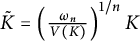 $\tilde {K}=\left (\frac {\omega _n}{V(K)}\right )^{1/n}K$
, that is,
 $\Phi _p(\tilde {K})\leq \mathcal R_p(\tilde K)\left (\frac {w(\tilde K)}{2}\right )^p=\mathcal R_p(K)\left (\frac {\omega _n^{1/n}}{V(K)^{1/n}}\frac {w(K)}{2}\right )^p$
holds. The desired result follows from Lemma 4.2, and the proof is finished.
5 Proof of Theorem 1.3
To prove Theorem 1.3, we need some preliminary results. We recall that the Santaló point
 $s(K)$
is the unique point such that
 $$ \begin{align*}V ((K-s(K))^\circ) =\inf_{z\in K} V((K-z)^\circ).\end{align*} $$
Lemma 5.1 For
 $p\in (1, n]$
and
 $n\geq 3$
, let
 $K\in \mathcal {K}_o^n$
with
 $V(K)=V(B_2^n)$
. Then
 $$ \begin{align*}\nonumber |e_p(K)-s(K)|^2\leq c_0(1-\Phi_{-p}(K))D(K)^{p+2}. \end{align*} $$
Here,
 $e_p$
is the extremum of
 $\Phi _p(K)$
in Definition 4.1,
 $D(K)$
denotes the diameter of K and
 $c_0=\frac {2n}{p(p+1)}$
.
Proof We assume
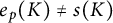 $e_p(K)\neq s(K)$
, since the conclusion is trivial if
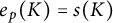 $e_p(K)= s(K)$
. We set
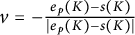 $v=-\frac {e_p(K)-s(K)}{|e_p(K)- s(K)|}$
and
 $$ \begin{align*}e(t)=e_p(K)+tv, \;\; t\in\left[0, \left|e_p(K)- s(K)\right|\right].\end{align*} $$
Denote by
 $h_t$
the support function of
 $K-e(t)$
and
 $$ \begin{align*}\phi(t)=\frac{1}{n\omega_n}\int_{S^{n-1}}h_t^{-p}\mathrm{d}\sigma.\end{align*} $$
It is not hard to see that
 $\phi (0)=\Phi _{-p}(K),\; \phi '(0)=0$
and
 $$ \begin{align*}\phi^{"}(t)=\frac{p(p+1)}{n\omega_n}\int_{S^{n-1}}h_t^{-p-2}(u)(u\cdot v)^2\mathrm{d}\sigma(u).\end{align*} $$
Combining
 $h_t\leq D(K)$
with the Taylor expansion of
 $\phi (t)$
around the point
 $t=0$
, it yields
 $$ \begin{align*}D(K)^{-p-2}|e_K(K)-s(K)|^2\leq c_0\left(\frac{1}{n\omega_n}\int_{S^{n-1}}h_{K-s(K)}^{-p}\mathrm{d}\sigma - \Phi_{-p}(K)\right)\leq c_0\left(1 - \Phi_{-p}(K)\right).\end{align*} $$
Here,
 $c_0^{-1}=\frac {p(p+1)}{2n\omega _n}\int _{S^{n-1}}(u\cdot v)^2du=\frac {p(p+1)}{2n}$
. The above second inequality comes from the fact that
 $\Phi _p(\tilde {K})\leq 1$
when
 $p\in [-n,0)$
, provided in [Reference Ivaki30]. Therefore, we have
 $$ \begin{align*}|e_K(K)-s(K)|^2\leq c_0\left(1 - \Phi_{-p}(K)\right)D(K)^{p+2}.\\[-33pt]\end{align*} $$
We now proceed to prove local stability of
 $L_p$
torsional measure by employing
 $L^{c_1}$
-distance (
 $c_1=\max \left \{n/(n-p), n/p\right \}$
) between two convex bodies.
We first recall the quantitative Young inequality given by Cianchi [Reference Cianchi14], that is, if
 $r\geq 2$
, and
 $\frac {1}{r}+\frac {1}{r'}=1$
, then
 $$ \begin{align} uv\leq \frac{1}{r}u^r+\frac{1}{r'}v^{r'}-\frac{1}{r}\left\lvert u-v^{\frac{1}{r-1}}\right\lvert^r\text{ for every }u,v\geq 0. \end{align} $$
An application of inequality (5.1) implies the following stability version of Hölder’s inequality.
Lemma 5.2 Let
 $1<a<\infty $
and b be its conjugate exponent, that is,
 ${\frac {1}{a}}+{\frac {1}{b}}=1$
. If
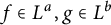 $f\in L^a, g\in L^b$
,
 $\|f\|_{a}, \|g\|_{b}>0$
, and
 $a\in [2, \infty )$
, then
 $$ \begin{align} \left\|fg\right\|_{1}\leq \|f\|_{a}\|g\|_{b}\left(1-{\frac{1}{a}}\left\|\frac{|f|}{\|f\|_{a}} -\left(\frac{|g|}{\|g\|_{b}}\right)^{\frac{1}{a-1}} \right\|_{a}^a\right). \end{align} $$
While if
 $a\in (1, 2]$
, it only needs to exchange the positions of a and b in the preceding inequality.
Proof Suppose
 $a\in [2, \infty )$
. We set
 $u=|f(x)|$
and
 $v=|g(x)|$
in inequality (5.1), then we get
 $$ \begin{align*} |f(x)||g(x)|\leq {\frac{1}{a}}|f(x)|^a+{\frac{1}{b}}|g(x)|^{b}-{\frac{1}{a}}\left\lvert |f(x)|-|g(x)|^{\frac{1}{a-1}}\right\lvert^a. \end{align*} $$
Then substituting
 $tf(x)$
for
 $f(x)$
and setting
 $t=\frac {\|g\|_{b}^{\frac {1}{a-1}}}{\|f\|_{a}}$
, it holds
 $$ \begin{align*} \frac{\|g\|_{b}^{\frac{1}{a-1}}}{\|f\|_{a}}|f(x)||g(x)| &\leq {\frac{1}{a}}{\frac{\|g\|_{b}^{b}}{\|f\|_{a}^a}}|f(x)|^a+{\frac{1}{b}}|g(x)|^b-{\frac{1}{a}}\left\lvert {\frac{\|g\|_{b}^{\frac{1}{a-1}}}{\|f\|_{a}}}|f(x)|-|g(x)|^{\frac{1}{a-1}}\right\lvert^a\\&=\|g\|_{b}^{b}\left({\frac{1}{a}}{\frac{|f(x)|^a}{\|f\|_{a}^a}}+{\frac{1}{b}}{\frac{|g(x)|^b}{\|g\|_{b}^{b}}}-{\frac{1}{a}}\left\lvert {\frac{|f(x)|}{\|f\|_{a}}}-\left({\frac{|g(x)|}{\|g\|_{b}}}\right)^{\frac{1}{a-1}}\right\lvert^a\right), \end{align*} $$
as well as
 $$ \begin{align*} |f(x)||g(x)|\leq \|f\|_{a}\|g\|_{b}\left({\frac{1}{a}}{\frac{|f(x)|^a}{\|f\|_{a}^a}}+{\frac{1}{b}}{\frac{|g(x)|^b}{\|g\|_{b}^{b}}}-{\frac{1}{a}}\left\lvert {\frac{|f(x)|}{\|f\|_{a}}}-\left({\frac{|g(x)|}{\|g\|_{b}}}\right)^{\frac{1}{a-1}}\right\lvert^a\right). \end{align*} $$
Integrating two sides of the above inequality, it implies
 $$ \begin{align*} \left\|fg\right\|_{1}\leq \|f\|_{a}\|g\|_{b}\left(1-{\frac{1}{a}}\left\|{\frac{|f|}{\|f\|_{a}}} -\left({\frac{|g|}{\|g\|_{b}}}\right)^{\frac{1}{a-1}} \right\|_{a}^a\right). \end{align*} $$
If
 $a\in (1, 2]$
, just interchange the roles of a and b, since
 $a,b$
are Hölder conjugates.
Theorem 5.3 Let
 $p\in (0,n)$
,
 $n\geq 3$
, and
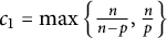 $c_1=\max \left\{\frac {n}{n-p}, \frac {n}{p}\right\}$
. If
 $K\in \mathcal {F}_o^n$
with
 $\Phi _{-p}(\tilde {K})\geq 1-\varepsilon $
for some
 $\varepsilon \in (0,1)$
, and
 $B_2^n(r_0))\subset \tilde {K}-s(\tilde {K})$
for some
 $0< r_0\leq 1$
, then there exists
 $B^n_2(r)$
such that
 $$ \begin{align*}\delta_{c_1}(\tilde{K}-e_p(\tilde{K}),B^n_2(r)) \leq C_1 \omega_n^{\frac{1}{c_1}}\varepsilon^{\frac{1}{2}},\end{align*} $$
where
 $$ \begin{align*}C_1=\left(c_1^{c_1+1}n^{1-c_1}D(K)^n\left(\max\left\{r_0^{-1}, D(\tilde K)\right\}\right)^{|n-c_1|}\right)^{\frac{1}{c_1}} + n^{\frac{1}{c_1}}\left(c_0D(\tilde{K})^{p+2}\right)^{\frac{1}{2}},\end{align*} $$
 $$ \begin{align*}1\leq r\leq (1-\varepsilon)^{-\frac{1}{p}},\end{align*} $$
and
 $c_0$
is the constant from Lemma 5.1 and
 $D(\tilde {K})$
denotes the diameter of
 $\tilde {K}$
.
In particular, if
 $\tilde {K}$
is origin-symmetric, then
 $$ \begin{align*}\delta_{c_1}(\tilde{K},B^n_2(r))^{c_1} \leq c_1^{c_1+1}n^{1-c_1}\omega_n\left(\frac{1}{2}D(\tilde{K})\right)^n\left(\max\left\{r_0^{-1}, \frac{1}{2}D(\tilde{K})\right\}\right)^{|n-c_1|}\varepsilon^{\frac{c_1}{2}}.\end{align*} $$
Proof We may assume
 $V(K)=V(B_2^n)$
without loss of generality. Denote by
 $h_e$
the support function of
 $K-e_p(K)$
and
 $h_s$
the support function of
 $K-s(K)$
. Since
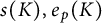 $s(K), e_p(K)$
are in the interior of K, the functions
 $h_e$
and
 $h_s$
are both positive.
We divide the proof into two cases:
 $n\geq 2p$
and
 $3\leq n <2p$
. In the case
 $n\geq 2p$
, we consider the functions
 $$ \begin{align*}f=h_s^{-p},~~g=1\end{align*} $$
and the constants
 $$ \begin{align*}a=\frac{n}{p},~~b=\frac{n}{n-p}.\end{align*} $$
By Lemma 5.2, one has
 $$ \begin{align*} \left\|fg\right\|_{1}\leq \|f\|_{a}\|g\|_{b}\left(1-{\frac{1}{a}}\left\|\frac{|f|}{\|f\|_{a}} -\left(\frac{|g|}{\|g\|_{b}}\right)^{\frac{1}{a-1}} \right\|_{a}^a\right). \end{align*} $$
By computing the terms of the above inequality, we get
 $$ \begin{align*} \|fg\|_{1}=&\int_{S^{n-1}}h_s^{-p}\mathrm{d}\sigma,\\ \|f\|_{a}=&\left(\int_{S^{n-1}}h_s^{{-p}\cdot \frac{n}{p}}\mathrm{d}\sigma\right)^{\frac{p}{n}} =\left(\int_{S^{n-1}}h_s^{-n}\mathrm{ d}\sigma\right)^{\frac{p}{n}},\\ \|g\|_{b}=&(n\omega_n)^{\frac{n-p}{n}}. \end{align*} $$
This implies that
 $$ \begin{align*} \frac{\int_{S^{n-1}}h_s^{-p}\mathrm{d}\sigma}{\left(\int_{S^{n-1}}h_s^{-n}\mathrm{ d}\sigma\right)^{\frac{p}{n}}(n\omega_n)^{\frac{n-p}{n}}} &\leq 1-{\frac{1}{a}}\left\|\frac{h_s^{-p}}{\left(\int_{S^{n-1}}h_s^{-n}\mathrm{ d}\sigma\right)^{\frac{p}{n}}} -\left(\frac{1}{(n\omega_n)^{\frac{n-p}{n}}}\right)^{\frac{p}{n-p}}\right\|_{a}^a\\ &=1-{\frac{1}{a}}\left\|\left(\frac{h_s^{-n}}{\int_{S^{n-1}}h_s^{-n}\mathrm{d}\sigma}\right)^{{\frac{1}{a}}} -\left(\frac{1}{n\omega_n}\right)^{{\frac{1}{a}}}\right\|_{a}^a. \end{align*} $$
In the case
 $3\leq n\leq 2p$
, putting
 $$ \begin{align*}f=1,~~g(\cdot)=h_s^{-p}, \text{ and } a=\frac{n}{p},~~b=\frac{n}{n-p},\end{align*} $$
we obtain
 $$ \begin{align*}\frac{\int_{S^{n-1}}h_s^{-p}\mathrm{d}\sigma}{\left(\int_{S^{n-1}}h_s^{-n}\mathrm{ d}\sigma\right)^{\frac{p}{n}}(n\omega_n)^{\frac{n-p}{n}}} \leq 1-{\frac{1}{b}}\left\|\left(\frac{h_s^{-n}}{\int_{S^{n-1}}h_s^{-n}\mathrm{ d}\sigma}\right)^{{\frac{1}{b}}} -\left(\frac{1}{n\omega_n}\right)^{{\frac{1}{b}}}\right\|_{b}^b.\end{align*} $$
To sum up, we come to
 $$ \begin{align} \frac{\int_{S^{n-1}}h_s^{-p}\mathrm{d}\sigma}{\left(\int_{S^{n-1}}h_s^{-n}\mathrm{ d}\sigma\right)^{\frac{p}{n}}(n\omega_n)^{\frac{n-p}{n}}} \leq 1-\frac{1}{c_1}\left\|\left(\frac{h_s^{-n}}{\int_{S^{n-1}}h_s^{-n}\mathrm{ d}\sigma}\right)^{\frac{1}{c_1}} -\left(\frac{1}{n\omega_n}\right)^{\frac{1}{c_1}}\right\|_{c_1}^{c_1}, \end{align} $$
where
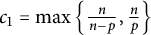 $c_1=\max \left\{\frac {n}{n-p},\frac {n}{p}\right\}$
.
By the assumption
 $\Phi _{-p}(K)\geq 1-\varepsilon $
, it follows from
 $$ \begin{align} \int_{S^{n-1}}h_s^{-p}\mathrm{d}\sigma\geq\int_{S^{n-1}}h_{e}^{-p}\mathrm{d}\sigma\geq n\omega_n(1-\varepsilon). \end{align} $$
Using the Blaschke-Santaló inequality and the fact that
 $V(K)=\omega _n$
, it holds
 $$ \begin{align*} \frac{\omega_n}{n}\int_{S^{n-1}}h_s^{-n}\mathrm{d}\sigma=V(K)V\left((K-s(K))^\circ\right) \leq\omega_n^2, \end{align*} $$
and thus
 $$ \begin{align} \frac{1}{n\omega_n}\int_{S^{n-1}}h_s^{-n}\mathrm{d}\sigma \leq 1. \end{align} $$
 $$ \begin{align} \frac{\int_{S^{n-1}}h_s^{-p}\mathrm{d}\sigma}{\left(\int_{S^{n-1}}h_s^{-n}\mathrm{ d}\sigma\right)^{\frac{p}{n}}(n\omega_n)^{\frac{n-p}{n}}} \geq1-\varepsilon. \end{align} $$
By (5.3) and (5.4), we have that
 $$ \begin{align*} n\omega_n(1-\varepsilon)\leq \int_{S^{n-1}}h_s^{-p}\mathrm{d}\sigma\leq \left(\int_{S^{n-1}}h_s^{-n}\mathrm{ d}\sigma\right)^{\frac{p}{n}}(n\omega_n)^{\frac{n-p}{n}}, \end{align*} $$
then,
 $$ \begin{align} (1-\varepsilon)^{\frac{1}{p}}\leq\left(\frac{1}{n\omega_n}\int_{S^{n-1}}h_s^{-n}\mathrm{d}\sigma\right)^{\frac{1}{n}}. \end{align} $$
Combining (5.3) with (5.6), we obtain
 $$ \begin{align} \left\|\left(\frac{h_s^{-n}}{\int_{S^{n-1}}h_s^{-n}\mathrm{d}\sigma}\right)^{\frac{1}{c_1}} -\left(\frac{1}{n\omega_n}\right)^{\frac{1}{c_1}}\right\|_{c_1}^{c_1} \leq c_1\varepsilon. \end{align} $$
Letting
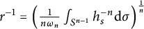 $r^{-1}=\left(\frac {1}{n\omega _n}\int _{S^{n-1}}h_s^{-n}\mathrm {d}\sigma \right)^{\frac {1}{n}}$
, it follows from (5.8) that for small
 $\varepsilon>0$
,
 $$ \begin{align} \left\|h_s^{\frac{n}{c_1}}-r^{\frac{n}{c_1}}\right\|_{c_1}^{c_1} \leq c_1 n\omega_n D(K)^n \varepsilon\leq c_1 n\omega_n D(K)^n \varepsilon^{\frac{c_1}{2}}, \end{align} $$
where
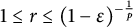 $1\leq r\leq (1-\varepsilon )^{-\frac {1}{p}}$
, by using (5.5) and (5.7). By virtue of the monotonicity of the derivative of the function
 $\phi (t)=t^{\frac {n}{c_1}}$
and the mean value theorem, it can be obtained that
 $$ \begin{align*} \lvert h_s^{\frac{n}{c_1}}-r^{\frac{n}{c_1}}\rvert\geq k\lvert h_s-r\rvert, \end{align*} $$
where
 $$ \begin{align*}\nonumber k = \begin{cases} \frac{n}{c_1}\left(\min\{h_s, r\}\right)^{\frac{n}{c_1}-1} & \text{ if } \frac{n}{c_1}\geq 1, \\ \frac{n}{c_1}\left(\max\{h_s, r\}\right)^{\frac{n}{c_1}-1} & \text{ if } \frac{n}{c_1}< 1. \end{cases} \end{align*} $$
Therefore, when
 $\frac {n}{c_1}\geq 1$
, it holds that
 $k\geq \frac {n}{c_1}r_0^{\frac {n}{c_1}-1}$
with the assumption of
 $B_2^n(r_0)\subset K-s(K)$
for some
 $0<r_0\leq 1$
. When
 $\frac {n}{c_1} < 1$
,
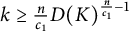 $k\geq \frac {n}{c_1}D(K)^{\frac {n}{c_1}-1}$
since
 $r=||h_s||_{L^{-n}(S^{n-1})}$
by the definition of r. To sum up, it follows that
 $$ \begin{align} \|h_s-r\|_{c_1}\leq \left(c_1^{c_1+1}n^{1-c_1}\omega_nD(K)^n\left(\max\left\{r_0^{-1}, D(K)\right\}\right)^{|n-c_1|}\right)^{\frac{1}{c_1}}\varepsilon^{\frac{1}{2}}. \end{align} $$
Moreover, by Lemma 5.1, we have
 $$ \begin{align*}|e_p(K)-s(K)| \leq \left(c_0D(K)^{p+2}\varepsilon\right)^{\frac{1}{2}}.\end{align*} $$
Hence,
 $$ \begin{align*}\left\|h_e-r\right\|_{c_1}\leq \left(c_1^{c_1+1}n^{1-c_1}\omega_nD(K)^n\left(\max\left\{r_0^{-1}, D(K)\right\}\right)^{|n-c_1|}\right)^{\frac{1}{c_1}}\varepsilon^{\frac{1}{2}} + (n\omega_n)^{\frac{1}{c_1}}\left(c_0D(K)^{p+2}\varepsilon\right)^{\frac{1}{2}}.\end{align*} $$
This completes the proof.
In the case that K is origin-symmetric, it has
 $$ \begin{align} |e_p(K)-s(K)|=0. \end{align} $$
Moreover, we can replace
 $D(K)$
by
 $\frac {1}{2}D(K)$
since
 $D(K)$
has been used to estimate the support function
 $h_K$
and
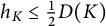 $h_K\leq \frac {1}{2}D(K)$
when K is origin-symmetric. The result for origin-symmetric case follows from (5.10) and (5.11).
Based on these preparations, we next give the stability proof for
 $1<p<n$
as follows.
Proof of Theorem 1.3.
Let
 $1<p<n$
. We first consider the case
 $V(K)=V(B_2^n)$
. Define
 $\Psi _p: \mathcal {F}_o^n \to (0,\infty )$
by
 $$ \begin{align*}\Psi_p(h_L)=\frac{\left(\int_{S^{n-1}}h_L^p\mathrm{d}\sigma\right)^{\frac{\alpha}{p}}}{\tau(L)}.\end{align*} $$
Combining the definition of functional derivative [Reference Engel and Dreizler18, p. 406] with (3.7), we have
 $$ \begin{align*} \frac{\mathrm{d}\tau(K)}{\mathrm{d} h_K}=|\nabla u|^2f_K. \end{align*} $$
Therefore, we obtain
 $$ \begin{align*}\nonumber \begin{aligned} (\mathrm{grad}\Psi_p)(h_K)&=\frac{\alpha h_K^{p-1}\left(\int_{S^{n-1}}h_K^p\mathrm{d}\sigma\right)^{\frac{\alpha}{p}-1}\tau(K)-|\nabla u|^2f_K \left(\int_{S^{n-1}}h_K^p\mathrm{d}\sigma\right)^{\frac{\alpha}{p}}}{\tau(K)^2}\\ &=\frac{h_K^{p-1}\left(\int_{S^{n-1}}h_K^p\mathrm{ d}\sigma\right)^{\frac{\alpha}{p}}}{\tau(K)^2}\left[\frac{\alpha\tau(K)}{\int_{S^{n-1}}h_K^p\mathrm{d}\sigma}-|\nabla u|^2h_K^{1-p}f_K\right]. \end{aligned} \end{align*} $$
By Łojasiewcz inequality, see [Reference Simon48, Section 3.13(ii)] and [Reference Simon48, p. 80], there exist
 ${c_2, \delta>0}$
, such that for any K with
 $\|h_K-1\|_{C^3}<\delta $
, it holds
 $$ \begin{align*}\left|\Psi_p(K)-\Psi_p(B_2^n)\right|^{\frac{1}{2}}\leq c_2\left\|(\mathrm{grad} \Psi_p)(h_K)\right\|_{2}.\end{align*} $$
Assuming
 $m\leq |\nabla u|^2h_K^{1-p}f_K\leq M, $
 $$ \begin{align*}m\int_{S^{n-1}}h_K^p\mathrm{d}\sigma\leq \int_{S^{n-1}}h_K^p|\nabla u|^2h_K^{1-p}f_K\mathrm{d}\sigma=\alpha\tau(K)\leq M\int_{S^{n-1}}h_K^p\mathrm{d}\sigma,\end{align*} $$
we can easily get
 $$ \begin{align*}\left|\frac{\alpha\tau(K)}{\int_{S^{n-1}}h_K^p\mathrm{d}\sigma}-|\nabla u|^2h_K^{1-p}f_K\right|\leq M-m.\end{align*} $$
By the definition of
 $\Psi _p$
,
 $$ \begin{align*}\nonumber \begin{aligned} \Psi_p(K)-\Psi_p(B_2^n)&=\frac{\left(\int_{S^{n-1}}h_K^p\mathrm{d}\sigma\right)^{\frac{\alpha}{p}}}{\tau(K)}-\frac{\left(\int_{S^{n-1}} \mathrm{d}\sigma\right)^{\frac{\alpha}{p}}}{\tau(B_2^n)}\\ &=\frac{(n\omega_n)^{\frac{\alpha}{p}}}{\tau(K)}\left(\frac{\omega(K)}{2}\right)^\alpha\left[\left(\frac{2}{\omega(K)}\right)^\alpha\left(\frac{1}{n\omega_n}\int_{S^{n-1}}h_K^p\mathrm{ d}\sigma\right)^{\frac{\alpha}{p}}-\frac{\tau (K)}{\tau\left(\frac{\omega(K)}{2}B_2^n\right)}\right]\\ &\geq \left(\frac{\omega(K)}{2}\right)^\alpha \frac{(n\omega_n)^{\frac{\alpha}{p}}}{\tau(K)}\left[\left(\frac{2}{\omega(K)}\right)^\alpha\left(\frac{1}{n\omega_n}\int_{S^{n-1}}h_K^p\mathrm{ d}\sigma\right)^{\frac{\alpha}{p}}-1 \right], \end{aligned} \end{align*} $$
where the last inequality holds due to the Urysohn type inequality (3.12). Hence,
 $$ \begin{align*}\nonumber \begin{aligned} &\left(\frac{2}{\omega(K)}\right)^\alpha\left(\frac{1}{n\omega_n}\int_{S^{n-1}}h_K^p\mathrm{d}\sigma\right)^{\frac{\alpha}{p}}-1 \\ \leq &\left(\frac{2}{\omega(K)}\right)^\alpha \frac{\tau(K)}{(n\omega_n)^{\frac{\alpha}{p}}}(\Psi_p(K)-\Psi_p(B_2^n))\\ \leq &\left(\frac{2}{\omega(K)}\right)^\alpha\frac{\tau(K)}{(n\omega_n)^{\frac{\alpha}{p}}}c_2^2\left\|(\mathrm{grad} \Psi_p)(h_K)\right\|_{2}^2\\ \leq&\left(\frac{2}{\omega(K)}\right)^\alpha \frac{\tau(K)}{(n\omega_n)^{\frac{\alpha}{p}}}c_2^2\left[\frac{(\int_{S^{n-1}}h_K^p\mathrm{ d}\sigma)^{\frac{\alpha}{p}}}{\tau(K)^2}(M-m)\right]^2\left\|h_K^{p-1}\right\|_{2}^2\\ =&\left(\frac{2}{\omega(K)}\right)^\alpha\frac{\tau(K)}{(n\omega_n)^{\frac{\alpha}{p}}}c_2^2\left[\frac{(\int_{S^{n-1}}h_K^p\mathrm{ d}\sigma)^{\frac{\alpha}{p}}}{\tau(K)^2}\cdot m\left(\frac{M}{m}-1 \right)\right]^2\left\|h_K^{p-1}\right\|_{2}^2. \end{aligned} \end{align*} $$
Due to
 $m\leq |\nabla u|^2h_K^{1-p}f_K$
, we know
 $$ \begin{align*}\frac{1}{\tau(K)} \leq \frac{\alpha}{m} \cdot \frac{1}{\int_{S^{n-1}}h_K^p\mathrm{d}\sigma}.\end{align*} $$
Therefore,
 $$ \begin{align*}\left(\frac{2}{\omega(K)}\right)^\alpha\left(\frac{1}{n\omega_n}\int_{S^{n-1}}h_{K}^p\mathrm{ d}\sigma\right)^{\frac{\alpha}{p}}-1 \leq C\left(\mathcal{R}_{p}(K)-1\right)^2,\end{align*} $$
where C is a universal constant by
 $\|h_K-1\|_{C^3}<\delta $
. Therefore, it follows that
 $\frac {1}{n\omega _n}\int _{S^{n-1}}h_{K}^p\mathrm {d}\sigma \leq \left(\frac {\omega (K)}{2}\right)^{p} \left(1+C\left(\mathcal {R}_{p}(K)-1\right)^2\right)^{\frac {p}{\alpha }}.$
This in turn implies that
 $$ \begin{align*}\Phi_{-p}(K)=\frac{1}{n\omega_n}\int_{S^{n-1}}h_{K}^{-p}\mathrm{d}\sigma\geq \left(\frac{1}{n\omega_n}\int_{S^{n-1}}h_{K}^p\mathrm{d}\sigma\right)^{-1}\geq \left(\frac{\omega(K)}{2}\right)^{-p} \left(1+C\left(\mathcal{R}_{p}(K)-1\right)^2\right)^{-\frac{p}{\alpha}}\end{align*} $$
by Jensen inequality.
If
 $V(K)\neq V(B_2^n)$
, we only need to replace K by
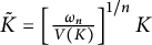 $\tilde {K}=\left[\frac {\omega _n}{V(K)}\right]^{1/n}K$
and then
 $$ \begin{align*} \Phi_{-p}(\tilde{K})\geq& \left(\frac{\omega(\tilde{K})}{2}\right)^{- p} \left(1+C\left(\mathcal{R}_{p}(\tilde{K})-1\right)^2\right)^{-\frac{p}{\alpha}}\\ =&\left(\frac{\omega_n^{1/n}\omega(K)}{2V(K)^{1/n}}\right)^{- p} \left(1+C\left(\mathcal{R}_{p}(K)-1\right)^2\right)^{-\frac{p}{\alpha}}. \end{align*} $$
We can complete the proof by using Theorem 5.3.
6 Proof of Theorem 1.4
In this section, we employ the stability version of the reverse Hölder inequality to complete the proof of Theorem 1.4, which establishes the global stability of the
 $L_p$
torsional measure for
 $p> n$
with
 $p \neq n+2$
. The stability of the reverse Hölder inequality, as established by Aldaz [Reference Aldaz2, Theorem 1], states the following lemma.
Lemma 6.1 Let
 $0<a<1$
, and let
 $b=a/(a-1)$
be its conjugate exponent. If
 $k\in L^b$
,
 $hk\in L^1$
, and
 $\|h\|_a,\|k\|_b>0$
, then for
 $1/2\leq a<1$
,
 $$ \begin{align*}\|h\|_{a} \|k\|_{b} \leq \|hk\|_{1} \left(1-(1-a)\left\|\frac{h^{1/2}k^{1/2}}{\left\|h^{1/2}k^{1/2}\right\|_{2}} -\frac{k^{b/2}}{\left\|k^{b/2}\right\|_{2}}\right\|_{2}^2\right)^{{\frac{1}{a}}}, \end{align*} $$
while for
 $0<a\leq 1/2$
, the terms a and
 $1-a$
exchange their positions in the preceding inequality.
By employing the stability result of the reverse Hölder inequality provided in Lemma 6.1, we can establish the corresponding stability for the
 $L_p$
-width functional
 $\Phi _p(\cdot )$
for
 $p>n$
, as presented in Theorem 6.2.
Theorem 6.2 Let
 $p>n$
and
 $\varepsilon \in (0,1)$
. If
 $K\in \mathcal {F}_o^n$
satisfies
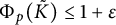 $\Phi _p(\tilde {K})\leq 1+\varepsilon $
with
 ${e_p(K)=0}$
, and
 $B_2^n(r_0)\subset \tilde {K}$
for some
 $0< r_0\leq 1$
, then there exist
 $B_2^n(r)$
with
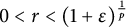 $0<r<(1+\varepsilon )^{\frac {1}{p}}$
, and a constant C depending on
 $r_0,p, n$
, and the diameter
 $D(K)$
of K, such that
 $$ \begin{align*}\delta_2(\tilde{K},B^n_2(r))^2\leq C(1+\varepsilon)^2 \left(1-\left(1+\varepsilon\right)^{-\frac{n}{p}}\right).\end{align*} $$
Furthermore, if p is an integer, the constant C only depends on n and
 $D(K)$
.
Proof Assume
 $V(K)=V(B_2^n)$
without loss of generality.
In the case of
 $n<p\leq 2n$
, we put
 $$ \begin{align*}h=h_K^{p}, k=1,a=\frac{n}{p}, b=\frac{n}{n-p}.\end{align*} $$
Then we have
 $a \in [\frac {1}{2},1)$
. Lemma 6.1 gives
 $$ \begin{align} \|h\|_{a} \|k\|_{b} \leq \|hk\|_{1} \left(1-(1-a)\left\|\frac{h^{1/2}k^{1/2}}{\left\|h^{1/2}k^{1/2}\right\|_{2}} -\frac{k^{b/2}}{\left\|k^{b/2}\right\|_{2}}\right\|_{2}^2\right)^{{\frac{1}{a}}}. \end{align} $$
By computing the terms in the preceding inequality, we have
 $$ \begin{align*} \|h\|_{a}=&\left(\int_{S^{n-1}}h_K^{{p}\cdot (\frac {n}{p})}\mathrm{d}\sigma\right)^{\frac{p}{n}}=\left(\int_{S^{n-1}}h_K^{n}\mathrm{ d}\sigma\right)^{\frac{p}{n}},\\ \|k\|_{b}=&(n\omega_n)^{\frac{n-p}{n}},\\ \|hk\|_{1}=&\left\|h_K^{p}\right\|_{1}=\int_{S^{n-1}}h_K^{p}\mathrm{d}\sigma. \end{align*} $$
Then in view of
 $\left\|h^{1/2}k^{1/2}\right\|_{2}=\left(\int _{S^{n-1}}h_K^{p}\mathrm {d}\sigma \right)^{\frac {1}{2}}$
and
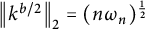 $\left\|k^{b/2}\right\|_{2}=(n\omega _n)^{\frac {1}{2}}$
, (6.1) implies that
 $$ \begin{align*}\frac{n\omega_n}{\int_{S^{n-1}}h_K^{p}\mathrm{d}\sigma}\left(\frac{\int_{S^{n-1}}h_K^{n}\mathrm{ d}\sigma}{n\omega_n}\right)^{\frac{p}{n}}\leq \left(1-(1-a)\left\|\frac{h_K^{\frac{p}{2}}}{\left(\int_{S^{n-1}}h_K^{p}\mathrm{ d}\sigma\right)^{\frac{1}{2}}} -\frac{1}{(n\omega_n)^{\frac{1}{2}}}\right\|_{2}^2\right)^{{\frac{1}{a}}}.\end{align*} $$
By the definition of
 $\Phi _p(K)$
with
 $e_p(K)=0$
, we have
 $$ \begin{align} \Phi_p(K)^{-\frac{n}{p}}\left(\frac{\int_{S^{n-1}}h_K^{n}\mathrm{d}\sigma}{n\omega_n}\right)\leq 1-(1-a)\left\|\frac{h_K^{\frac{p}{2}}}{\left(\int_{S^{n-1}}h_K^{p}\mathrm{d}\sigma\right)^{\frac{1}{2}}} -\frac{1}{(n\omega_n)^{\frac{1}{2}}}\right\|_{2}^2. \end{align} $$
In the case of
 $p\geq 2n$
, we put
 $$ \begin{align*}h=h_K^{\frac{pn}{p-n}}, k=h_K^{\frac{pn}{n-p}},a=\frac{n}{p}, b=\frac{n}{n-p}.\end{align*} $$
By
 $p\geq 2n$
, we have
 $a\in (0,\frac {1}{2}]$
. If we denote by
 $a'=1-a=(p-n)/p$
,
 $b'=(n-p)/n$
, Lemma 6.1 gives
 $$ \begin{align} \|h\|_{a'} \|k\|_{b'} \leq \|hk\|_{1} \left(1-a'\left\|\frac{h^{1/2}k^{1/2}}{\left\|h^{1/2}k^{1/2}\right\|_{2}} -\frac{k^{{b'}/2}}{\left\|k^{b'/2}\right\|_{2}}\right\|_{2}^2\right)^{\frac{1}{a'}}. \end{align} $$
By computing the terms of the preceding inequality, we have
 $$ \begin{align*} \|h\|_{a'}=&\left(\int_{S^{n-1}}h_K^{\frac{pn}{p-n}\cdot \frac{p-n}{p}}\mathrm{ d}\sigma\right)^{\frac{p}{p-n}}=\left(\int_{S^{n-1}}h_K^{n}\mathrm{d}\sigma\right)^{\frac{p}{p-n}},\\ \|k\|_{b'}=&\left(\int_{S^{n-1}}h_K^{\frac{pn}{n-p}\cdot \frac{n-p}{n}}\mathrm{d}\sigma\right)^{\frac{n}{n-p}} =\left(\int_{S^{n-1}}h_K^{p}\mathrm{d}\sigma\right)^{\frac{n}{n-p}},\\ \|hk\|_{1}=&\left|1\right|_{1}=n\omega_n. \end{align*} $$
Thus, in view of
 $\left\|h^{1/2}k^{1/2}\right\|_{2}=(n\omega _n)^{\frac {1}{2}}$
and
 $\left\|k^{b'/2}\right\|_{2}=\left(\int _{S^{n-1}}h_K^{p}\mathrm {d}\sigma \right)^{\frac {1}{2}}$
, it follows from (6.3) that
 $$ \begin{align*}\left(\frac{1}{n\omega_n}\int_{S^{n-1}}h_K^{p}\mathrm{ d}\sigma\right)^{\frac{n}{n-p}}\left(\frac{1}{n\omega_n}\int_{S^{n-1}}h_K^{n}\mathrm{d}\sigma\right)^{\frac{p}{p-n}}\leq \left(1-a'\left\|\frac{h_K^{\frac{p}{2}}}{\left(\int_{S^{n-1}}h_K^{p}\mathrm{d}\sigma\right)^{\frac{1}{2}}} -\frac{1}{(n\omega_n)^{\frac{1}{2}}}\right\|_{2}^2\right)^{\frac{p}{p-n}}.\end{align*} $$
By the definition of
 $\Phi _p(K)$
, we have
 $$ \begin{align} \Phi_p(K)^{-\frac{n}{p}}\left(\frac{1}{n\omega_n}\int_{S^{n-1}}h_K^{n}\mathrm{d}\sigma\right)\leq 1-a'\left\|\frac{h_K^{\frac{p}{2}}}{\left(\int_{S^{n-1}}h_K^{p}\mathrm{d}\sigma\right)^{\frac{1}{2}}} -\frac{1}{(n\omega_n)^{\frac{1}{2}}}\right\|_{2}^2. \end{align} $$
Let
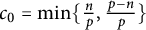 $c_0=\min \{\frac {n}{p},\frac {p-n}{p}\}$
. It follows from (6.2) and (6.4) that
 $$ \begin{align} \Phi_p(K)^{-\frac{n}{p}}\left(\frac{1}{n\omega_n}\int_{S^{n-1}}h_K^{n}\mathrm{d}\sigma\right)\leq 1-c_0\left\|\frac{h_K^{\frac{p}{2}}}{\left(\int_{S^{n-1}}h_K^{p}\mathrm{d}\sigma\right)^{\frac{1}{2}}} -\frac{1}{(n\omega_n)^{\frac{1}{2}}}\right\|_{2}^2. \end{align} $$
Using Jensen inequality and the classical Urysohn’s inequality (2.2) with the assumption
 $V(K)=V(B_2^n)$
, we can estimate that
 $$ \begin{align*}\frac{1}{n\omega_n}\int_{S^{n-1}}h_K^{n}\mathrm{d}\sigma\geq \left(\frac{1}{n\omega_n}\int_{S^{n-1}}h_K\mathrm{ d}\sigma\right)^n=1.\end{align*} $$
Using the above estimate and the assumption
 $\Phi _p(K)\leq 1+\varepsilon ,$
it follows from (6.5) that
 $$ \begin{align*} \left(1+\varepsilon\right)^{-\frac{n}{p}}\leq 1-c_0\left\|\frac{h_K^{\frac{p}{2}}}{\left(\int_{S^{n-1}}h_K^{p}\mathrm{ d}\sigma\right)^{\frac{1}{2}}} -\frac{1}{(n\omega_n)^{\frac{1}{2}}}\right\|_{2}^2, \end{align*} $$
for any
 $p\geq n$
. Then we have
 $$ \begin{align*} \left\|h_K^{\frac{p}{2}}-\left(\frac{\int_{S^{n-1}}h_K^{p}\mathrm{d}\sigma}{n\omega_n} \right)^{\frac{1}{2}}\right\|_{2}^2 \leq \frac{\left(\int_{S^{n-1}}h_K^{p}\mathrm{d}\sigma\right)}{c_0} \left(1-\left(1+\varepsilon\right)^{-\frac{n}{p}}\right). \end{align*} $$
If we denote by
 $$ \begin{align*}r^p=\frac{1}{n\omega_n}\int_{S^{n-1}}h_K^{p}\mathrm{d}\sigma,\end{align*} $$
then
 $$ \begin{align} \left\|h_K^{\frac{p}{2}}-r^{\frac{p}{2}}\right\|_{2}^2 \leq \frac{n\omega_n(1+\varepsilon)}{c_0} \left(1-\left(1+\varepsilon\right)^{-\frac{n}{p}}\right), \end{align} $$
where
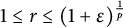 $1\leq r\leq (1+\varepsilon )^{\frac {1}{p}}$
, due to
 $1\leq \Phi _p(K)\leq 1+\varepsilon $
.
For
 $p> n$
, the function
 $f(t)=t^p$
is increasing and convex, and for
 $t_1\leq t_2$
,
 $$ \begin{align*}|f(t_2)-f(t_1)|\geq f'(t_1)|t_2-t_1|.\end{align*} $$
Thus, it implies that
 $$ \begin{align*} |h_K^{\frac{p}{2}}-r^{\frac{p}{2}}|\geq p\min \{r,h_K\}^{\frac{p-1}{2}} |h_K^{\frac{1}{2}}-r^{\frac{1}{2}}| \geq pr_0^{\frac{p-1}{2}} |h_K^{\frac{1}{2}}-r^{\frac{1}{2}}|, \end{align*} $$
where the latter inequality follows from the assumption of
 $B^n_2(r_0)\subset K$
for some
 ${0<r_0\leq 1}$
and the fact
 $$ \begin{align*}1\leq r=\Phi_p(K)^{\frac{1}{p}}\leq (1+\varepsilon)^{\frac{1}{p}}\leq 1+\varepsilon.\end{align*} $$
Furthermore, since
 $$ \begin{align*}|h_K^{\frac{1}{2}}-r^{\frac{1}{2}}|\geq \frac{|h_K-r|}{|h_K^{\frac{1}{2}}+r^{\frac{1}{2}}|}\geq\frac{|h_K-r|}{D(K)^{\frac{1}{2}}+(1+\varepsilon)^{\frac{1}{2}}},\end{align*} $$
we have
 $$ \begin{align*} |h_K^{\frac{p}{2}}-r^{\frac{p}{2}}|\geq \frac{pr_0^{\frac{p-1}{2}}}{D(K)^{\frac{1}{2}}+(1+\varepsilon)^{\frac{1}{2}}}|h_K-r|. \end{align*} $$
Here,
 $D(K)$
denotes the diameter of K; then it is obvious that
 $D(K)\geq h_K$
. This together with (6.6) shows that
 $$ \begin{align*} \left\|h_K-r\right\|_{2}^2 &\leq \frac{n\omega_n(1+\varepsilon)}{p^2c_0r_0^{p-1}}\left[D(K)^{\frac{1}{2}}+(1+\varepsilon)^{\frac{1}{2}}\right]^2 \left(1-\left(1+\varepsilon\right)^{-\frac{n}{p}}\right)\\ &\leq \frac{2n\omega_n(1+D(K))}{p^2c_0r_0^{p-1}}\left(1+\varepsilon\right)^2 \left(1-\left(1+\varepsilon\right)^{-\frac{n}{p}}\right), \end{align*} $$
where the second inequality holds due to
 $$ \begin{align*} (1+\varepsilon)\left[D(K)^{\frac{1}{2}}+(1+\varepsilon)^{\frac{1}{2}}\right]^2\leq 2(1+\varepsilon)(D(K)+(1+\varepsilon))\leq 2(1+\varepsilon)^2(D(K)+1). \end{align*} $$
Furthermore, using the assumption
 $\Phi _p(K)\leq 1+\varepsilon ,$
there exists a constant C depending on
 $r_0$
, p, n, and
 $D(K)$
, such that
 $$ \begin{align*} \delta_2(K,B^n_2(r))^2 \leq C(1+\varepsilon)^2 \left(1-\left(1+\varepsilon\right)^{-\frac{n}{p}}\right). \end{align*} $$
In addition, if
 $p=m$
is an integer, we have
 $$ \begin{align*} |h_K^{\frac{m}{2}}-r^{\frac{m}{2}}|\geq |h_K^{\frac{1}{2}}-r^{\frac{1}{2}}|=\frac{|h_K-r|}{|h_K^{\frac{1}{2}}+r^{\frac{1}{2}}|}, \end{align*} $$
since
 $r>1$
. Then, from (6.6), we have
 $$ \begin{align*} \left\|h_K-r\right\|_{2}^2 \leq \frac{2n\omega_n(1+D(K))}{c_0} \left(1+\varepsilon\right)^2\left(1-\left(1+\varepsilon\right)^{-\frac{n}{p}}\right). \end{align*} $$
Using the assumption
 $\Phi _p(K)\leq 1+\varepsilon ,$
there exists C depending on n and
 $D(K)$
, such that
 $$ \begin{align*} \delta_2(K,B^n_2(r))^2 \leq C(1+\varepsilon)^2 \left(1-\left(1+\varepsilon\right)^{-\frac{n}{p}}\right), \end{align*} $$
as wanted.
We are ready to give the proof of Theorem 1.4.
Proof of Theorem 1.4.
For the case
 $V(K)=\omega _n$
, we can get (4.3) by using the similar argument in Theorem 1.2, that is,
 $$ \begin{align*} \Phi_p(K)\leq \frac{1}{n\omega_n}\int_{S^{n-1}}h_K^p\mathrm{d}\sigma\leq \frac{M}{m}\left(\frac{w(K)}{2}\right)^p. \end{align*} $$
By the assumption of
 $e_p(K)=0$
, we quickly give the result
 $$ \begin{align*}\delta_2(K,B^n_2(r))^2\leq C\left(\frac{\omega(K)}{2}\right)^{2p}\mathcal{R}_{p}(K)^2 \left(1-\left(\frac{\omega(K)}{2}\right)^{-n}\mathcal{R}_{p}(K)^{-\frac{n}{p}}\right),\end{align*} $$
using Theorem 6.2.
In the general case where
 $V(K) \neq \omega _n$
, it suffices to consider K by
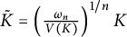 $\tilde {K}=\left(\frac {\omega _n}{V(K)}\right)^{1/n}K$
and hence
 $$ \begin{align*}\Phi_p(\tilde{K})\leq \mathcal R_p(\tilde K)\left(\frac{w(\tilde K)}{2}\right)^p=\mathcal R_p(K)\left(\frac{\omega_n^{1/n}}{V(K)^{1/n}}\frac{w(K)}{2}\right)^p.\end{align*} $$
Therefore, it holds that
 $$ \begin{align*}\delta_2(\tilde{K},B^n_2(r))^2\leq C\left(\frac{\omega_n^{1/n}}{V(K)^{1/n}}\frac{w(K)}{2}\right)^{2p}\mathcal{R}_{p}(K)^2 \left(1-\left(\frac{\omega_n^{1/n}}{V(K)^{1/n}}\frac{w(K)}{2}\right)^{-n}\mathcal{R}_{p}(K)^{-\frac{n}{p}}\right)\end{align*} $$
by Theorem 6.2. This completes the proof.



