Basis of the MR signal

The original term for the physical phenomenon that is the basis of both structural MRI and fMRI was nuclear MR, rather than simply MR (Bloch, Hansen, & Packard, Reference Bloch, Hansen and Packard1946; Purcell, Torrey, & Pound, Reference Purcell, Torrey and Pound1946). The original name captured key features of the phenomenon, specifically, that the nuclei of certain elements possess properties that, in the presence of a magnetic field, make them sensitive (resonant) to specific frequencies of magnetic oscillation. This is the foundation for all MR data collection. The word nuclear, which has certain negative connotations, is now commonly omitted when referring to MRI, in part because the method involves no sources of ionizing radiation (cf. computerized axial tomography and positron emission tomography [PET] scans, which use X-rays and radioisotopes, respectively). In essence, MRI involves transmitting small amounts of tuned energy into a sample of interest (e.g., a brain) in the presence of a strong magnetic field, allowing some of that energy to be absorbed by the atomic nucleus of the element to which the energy has been tuned, and then observing any resonant signal released by the sample once the source of the tuned energy has been turned off (Jezzard & Clare, Reference Jezzard, Clare, Jezzard, Matthews and Smith2001; Purcell et al., Reference Purcell, Torrey and Pound1946). A useful analogy can be found in the use of a tuning fork to check the tuning of the strings in a piano. The tuning fork is struck and, while vibrating, is touched to the piano frame, sending energy into the piano's strings. Strings that are resonant to the frequency of the fork will begin to vibrate, whereas strings that are not tuned to that frequency will not vibrate or will do so less robustly. Once the tuning fork is removed, the strings in the piano that began to vibrate will continue to resonate until the energy they have absorbed has dissipated. It is this residual, or resonant, energy that is analogous to the signal measures in MRI.

There are many atomic nuclei that can be made to resonate for the purpose of generating an MR signal. The practical requirement is that there be an odd number of protons and neutrons in the nucleus of the element of interest (Young, Reference Young1988). Because it has a nucleus composed of a single proton and is also the most common element in the human body, hydrogen is ideal for obtaining a resonant response from virtually any site in the body (Huettel, Song, & McCarthy, Reference Huettel, Song and McCarthy2004; Mansfield & Pykett, Reference Mansfield and Pykett1978). Protons possess a property known as spin, which is an angular momentum, analogous to the rotational force found in a child's top or toy gyroscope. They also possess a magnetic dipole moment, similar to a small magnet with poles of opposite force. There are consequences of both the hydrogen proton's magnetic dipole moment and its spin when the proton is placed in the presence of an external magnetic field. One consequence is that the magnetic poles are drawn to orient with the poles of the external magnetic field, just as any other magnet would. Another consequence, however, is that because of the proton's spin, the magnetic dipole moment does not completely align itself to the external magnetic field. Instead, it precesses, or rotates, about the axis of the external magnetic field. This precession persists in the presence of the external magnetic field and is a critical component of the MR signal. (For an excellent review of the basis of the MR signal, see Buxton, Reference Buxton2002.)

Relaxation, free induction decay, and tissue differentiation

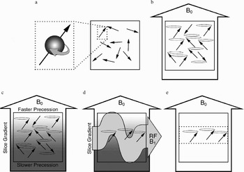
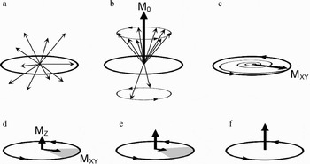
Prior to being introduced into the scanner magnet, the magnetic dipole moments of the hydrogen protons in a sample (e.g., a human body) are randomly oriented, and their spins are randomly out of phase, meaning that individual protons are at different points in their spin rotation (see Figures 1a and 2a). Once the sample is placed inside the scanner magnet, however, the magnetic dipole moments begin to orient themselves along the axis of the external, main magnetic field (which is labeled B₀, by convention) and begin to precess, but are still not in phase (see Figures 1b and 2b). Of course, when we measure these effects, we cannot do so at the microscopic level of individual dipole moments, but at a macroscopic level summing across the effects of many dipole moments. Thus, the local magnetization, M, of some portion of the sample, reflects the summed effect across the hydrogen protons in that portion of the sample. When the sample is initially placed into the scanner, in any given portion of the sample there is no local magnetization because the dipole moments have not yet had time to orient themselves with the magnetic field. However, with time, more and more of the dipole moments align to B₀, and the corresponding net local magnetization that is aligned along the scanner axis, M₀, increases until a steady state of equilibrium is reached (see Figure 2b). This process of coming to equilibrium is called relaxation, and its time course is described by a time constant known as T1.

Figure 1.

A schematic representation of a scan sample and its dipole moments in an MRI scanner. (a) Prior to being placed in the scanner, the dipole moments are randomly oriented throughout the sample (inset illustrates the spin and moment of a given proton). (b) Upon being placed in the scanner, the dipole moments in the sample probabilistically align with the main magnetic field (B₀). Note that at this point the dipole moments begin to precess at the same rate but are not yet in phase. (c) With the application of a secondary, slice-selective magnetic gradient (schematized here by the gradient shading) the moments precess at different rates along the gradient. (d) When an oscillating RF magnetic pulse (B₁) is applied to the sample, the dipole moments in the portion of the sample that are precessing at the optimal rate are brought into phase. (e) When the RF pulse ends, the dipole moments continue to precess in the selected slice (dotted box), although they immediately begin to fall out of phase.

Figure 2.

An illustration of the dipole moments at a representative location (e.g., a given slice) within a scan sample. (a) Prior to being placed in the scanner, the dipole moments are randomly oriented. (b) Upon being placed in the scanner, the dipole moments probabilistically align with the main magnetic field. The resulting net magnetization (M₀) is shown. Note that at this point the dipole moments begin to precess at the same rate but are not yet in phase. With the application of a secondary, slice-selective magnetic gradient the moments at this location in the sample precess at a unique frequency. (c) When an oscillating RF magnetic pulse that matches this frequency is applied to the sample, the dipole moments are brought into phase. As the RF pulse continues to be applied, M₀ tips away from the axis of the main magnetic field and spirals down toward the plane perpendicular to B₀. The portion of M₀ that precesses in this plane is labeled M_XY. In the figure, M₀ has been pushed 90° away from B₀. (d) When the RF pulse ends, M_XY continues to precess in the selected slice. This net magnetic precession induces a current in an adjacent wire coil, which is recorded as data. With time, however, the individual dipole moments are subject to random influences that drive them out of phase (indicated by the shaded grey region), resulting in a decrease in M_XY amplitude (note the decreasing amplitude of the M_XY component and the increasing amplitude of the M_Z component). (e) With time, the M_XY amplitude continues to decrease and the M_Z amplitude continues to increase. (f) Both T2 and T2* effects work to reduce the amplitude of M_XY after the RF pulse has been removed. As a consequence, M_XY loses amplitude faster than M_Z recovers. Thus, in the illustration, M_Z is not yet fully recovered at the point where the M_XY amplitude is minimal.

To prepare a particular slice of the sample for data collection, a secondary magnetic field is applied whose strength varies linearly across the magnet bore. This causes the dipole moments at different locations in the sample begin to precess at different frequencies (see Figure 1c; see further explanation in the MRI Data Collection Section). With the application of an additional oscillating magnetic field that is oriented perpendicular to B₀, the net local magnetization in the section of the sample precessing at that frequency can be pushed away from its alignment with B₀ (Bloch, Reference Bloch1946; Hahn, Reference Hahn1950). This oscillating field is known as the radiofrequency (RF) pulse and is labeled B₁ by convention. The application of the RF pulse is said to push or tip the net magnetization away from the axis of B₀ (see Figures 1d and 2c). How far down M₀ is pushed depends on the amplitude and duration of the RF pulse. Of importance, when M₀ is pushed out of alignment, this net magnetization begins to precess around the B₀ axis (similar to the precession of the individual dipole moments). It is this precession of the net magnetization in the sample that produces the transient, measurable signal that is recorded as data. The strongest signal will be produced when the net magnetization is largest, which occurs 90° from B₀.

Once M₀ has been pushed away from B₀, it can be thought of as having two separate components (see Figure 2d). The first is M_Z, which is aligned with B₀ and reflects the relaxation component of M₀. The more M₀ is tipped away from B₀, the smaller the amplitude of M_Z. The second is M_XY, which is perpendicular to B₀ and reflects both the extent to which M₀ has been pushed over (the more M₀ is pushed over, the larger the amplitude of M_XY becomes) and the degree to which the individual dipole moments are in phase with one another (the more in phase the dipole moments are, the greater M_XY is). As the M_XY component precesses, it acts like a local, moving magnetic field. Such a moving magnetic field will induce current flow in an adjacent coil of wire, and it is this induced current flow that we are measuring when we collect MR data.

If the dipole moments that comprise M_XY are in phase as they precess, the amplitude of M_XY is large, producing a strong data signal. However, if the dipole moments fall out of phase, the result is a net loss of M_XY magnetization, which produces a weaker data signal (see Figure 2e). After the RF pulse is turned off, the precession of each of the dipoles is no longer under the influence of B₁ and begins to be affected by random events that produce slight differences in the magnetization experienced by each dipole moment. These random events cause the dipoles to move out of phase with one another, resulting in an eventual loss of signal strength in the precessing M_XY. This is known as free induction decay, and the time constant associated with this decay is known as T2 (Bottomley, Foster, Argersinger, & Pfeiffer, Reference Bottomley, Foster, Argersinger and Pfeiffer1984; Bottomley, Hardy, Argersinger, & Allen-Moore, Reference Bottomley, Hardy, Argersinger and Allen-Moore1987).

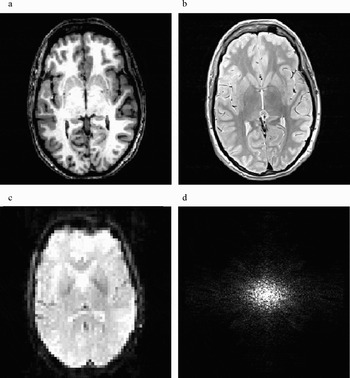
At this point we are ready to consider how different signal amplitudes can be obtained from different tissue types for the purpose of producing images that resolve anatomical structure. One way to do this is to simply record the differences in signal amplitude that occur among different tissue types as a consequence of differences in proton density. Tissue that is more proton dense, such as gray matter, will emit a stronger signal and will appear brighter on a resulting image as opposed to tissue that is less proton dense, such as white matter. Images of this type are known as proton density or density-weighted images. However, the differences in proton density between tissue types may not sufficiently emphasize the anatomical differences of interest to the researcher. An alternative strategy is to exploit the fact that different tissues in the body have different T1 and T2 time constants because of the nature of the substances in which the individual hydrogen nuclei are located. Two scan parameters that are relevant for exploiting these differences in time constants are the repetition time (or time to repeat [TR]) and the echo time (or time to echo [TE]). TR refers to the time between RF pulses used to excite the selected tissue. TE refers to the time delay between the RF pulse and the midpoint of the data collection period. By manipulating these and other components in the scan sequence it is possible to produce images with different contrast levels for different tissue types (Buxton, Edelman, Rosen, Wismer, & Brady, Reference Buxton, Edelman, Rosen, Wismer and Brady1987; McRobbie, Moore, Graves, & Prince, Reference McRobbie, Moore, Graves and Prince2003). Images that exploit differences in relaxation constants are known as T1-weighted images (see Figure 3a). Those that exploit differences in the decay of the M_XY magnetization are known as T2-weighted images (see Figure 3b). In essence, all MR images are a mixture of signal effects due to proton density, T1, and T2. Different scan sequences are designed to emphasize the influence of each of these factors and the effect each has in emphasizing the contrast of one tissue type over another.

Figure 3.

Examples of (a) a T1-weighted structural image, (b) a T2-weighted structural image, and (c) a T2*-weighted, echo planar imaging (EPI) functional image. (d) A representative illustration of k-space. Low-frequency, high-contrast information is located at the center of k-space.

Basis of the blood oxygen level dependent (BOLD) response and fMRI

Thus far our discussion has been limited to the production of structural images. However, many researchers will have as their primary objective the analysis of differences in functional brain activity between behavioral conditions or groups. Fortunately, there is a method for producing images in which contrast levels in different areas of the brain differ, not according to anatomical tissue type, but according to the level of oxygenation in the blood (Belliveau et al., Reference Belliveau, Kennedy, McKinstry, Buchbinder, Weisskoff and Cohen1991; Kwong et al., Reference Kwong, Belliveau, Chesler, Goldberg, Weisskoff and Poncelet1992; Ogawa, Lee, Nayak, & Glynn, Reference Ogawa, Lee, Nayak and Glynn1990; Turner, Le Bihan, Moonen, Despres, & Frank, Reference Turner, Le Bihan, Moonen, Despres and Frank1991). Red blood cells have been shown to have different magnetic properties depending on whether the hemoglobin molecule is oxygenated (in which case it is diamagnetic) or deoxygenated (in which case it is paramagnetic). The paramagnetic property of a deoxygenated blood cell causes greater distortion of the magnetic field that surrounds it in comparison to an oxygenated blood cell (i.e., the magnetic susceptibility, or magnetizability, of deoxygenated blood is greater than that of oxygenated blood). The greater local magnetic distortion associated with deoxygenated blood results in greater local dephasing effects, which results in a weaker local signal. The difference between the signal response to oxygenated and deoxygenated blood is known as the BOLD response. The local dephasing effects are known as BOLD T2* (or simply T2*) effects, and BOLD MRI images are said to be T2* weighted (see Figure 3c).

Because neuronal activity requires the consumption of oxygen as part of the metabolic process, local areas of neuronal firing will produce a decrease in available oxygen stores. The cerebral vasculature rapidly compensates for this local reduction in oxygen by increasing both the volume and flow of blood to areas of the brain that are active. This influx of fresh, oxygenated blood is overabundant, resulting, somewhat ironically, in an increase in local blood oxygen levels above those found at resting baseline (Fox, Raichle, Mintun, & Dence, Reference Fox, Raichle, Mintun and Dence1988; Raichle, Reference Raichle, Mountcastle, Plum and Geiger1987). Thus, in and around areas of neuronal activity, the change in blood flow that results in an increase in oxygenated blood also produces less distortion of the local magnetic field than when the area is at resting baseline. The result is that areas of increased neuronal activation show increases in signal amplitude compared to areas that are at rest, and are revealed as increases in brightness on the resulting brain images.

Although BOLD functional images are usually interpreted as reflecting differences in neural activity, it is important to remember that they are not direct measures of that activity. Data based on the BOLD response is an indirect measure of the vascular response to neural activity, and thus does not measure changes in the electrical, neurotransmitter, or metabolic functioning of neurons themselves. In addition, because the BOLD response is based on vascular changes that occur as a consequence of neural activity, the peak hemodynamic (blood flow and oxygenation) response following the presentation of a given stimulus lags behind the stimulus in time. Thus, data collected at the time of stimulus presentation reflect little or no influence of the stimulus event. Instead, the characteristic hemodynamic response curve peaks approximately 6 to 9 s after stimulus onset (DeYoe, Bandettini, Neitz, Miller, & Winans, Reference DeYoe, Bandettini, Neitz, Miller and Winans1994; Miezin, Maccotta, Ollinger, Petersen, & Buckner, Reference Miezin, Maccotta, Ollinger, Petersen and Buckner2000). Following stimulus offset, the signal again displays a lag before declining back to baseline. For a brief stimulus, the entire duration of the BOLD response, including full return to baseline, is on the order of approximately 10 to 16 s (Buckner & Braver, Reference Buckner, Braver, Moonen and Bandettini1999).

Scanner components

There are four pieces of physical hardware that lie at the heart of all current MRI systems (Huettel et al., Reference Huettel, Song and McCarthy2004): the main magnetic field coil, the shim coils, the RF coils, and the gradient coils (of which there are three). The main magnetic field coil is a very large electromagnet that forms the heart of the system. Its physical form is what determines the tube- or tunnel-like shape of most scanners, in which there is a central horizontal bore that runs the length of the scanner that is open at both ends. Typically, a patient or experiment participant lies supine on a cushioned platform or bed that can be moved in and out of the bore. The electromagnetic coil surrounds the scanner bore, and when electrical current is flowing through it, a powerful magnetic field exists, with its axis running parallel to the scanner bore. The strength of different magnets is determined by the main magnetic coil. Magnetic field strength is measured in teslas, where 1 tesla (T) is equivalent to 10,000 gauss (strength of the Earth's magnetic field at its surface = ~0.5 gauss). Most research and clinical scanners currently have a field strength of either 1.5 or 3.0 T. The large magnetic field generated by the main scanner magnet is possible in part because the main coil is supercooled, typically with liquid helium. One advantage of this, in addition to producing a very strong magnetic field, is that electrons flowing in the magnet coil encounter very little resistance, so that once the magnet has been cooled and electrified, the main magnetic field is self-sustaining, even after the external electrical current has been removed. This critical fact means that the scanner's main magnetic field is always present, even when the magnet is “off” and no data are being collected.

Given the omnipresence of such a powerful, silent, and invisible force, we cannot emphasize enough the importance of establishing and adhering to safety protocols to ensure that no ferromagnetic or paramagnetic materials are brought into the presence of the scanner's magnetic field by members of the research team or persons to be scanned. Objects containing ferromagnetic or paramagnetic materials may be drawn into the magnet bore, posing a serious safety hazard for anyone inside the magnet. Although they have been few in number, there are documented instances of objects flying into the magnet bore with such force that participant injury, and even death, has occurred (Chen, Reference Chen2001; Klucznik, Carrier, & Pyka, Reference Klucznik, Carrier and Pyka1993). In addition, ferromagnetic or paramagnetic objects inside or on the surface of the body may move or become heated when subjected to the various magnetic forces involved in an MRI scan (Kanal et al., Reference Kanal, Borgstede, Barkovich, Bell, Bradley and Etheridge2004). One need only consider the consequences of a moving or heating aneurism clip or of a malfunctioning pacemaker to imagine the seriousness of keeping persons with embedded metal objects away from the magnetic fields present in the scanner environment. Finally, the presence of even very small objects, such as a paper clip or staple, inside the magnet can produce large distortions in the main magnetic field that may affect data quality.

Although the ideal conditions for MRI involve a perfectly uniform main magnetic field, with equivalent magnetic force throughout the scanner bore, the reality is that this is impossible to attain. Even the insertion of the participant into the bore for the purpose of scanning introduces field inhomogeneities. Shim coils are electromagnetic coils embedded within the scanner housing that are capable of adjusting the main magnetic field so as to accommodate large field inhomogeneities that may be present because of imperfections in the static main magnetic field, as well as those introduced by the presence of the sample to be scanned (Reese, Davis, & Weisskoff, Reference Reese, Davis and Weisskoff1995). The presence and influence of these coils are largely invisible to the typical user, except at the beginning of a given scan sequence, when the scanner sends a test pulse to determine what field inhomogeneities are present and then adjusts the shim coils to produce a main magnetic field that is homogenous within some specified criterion.

To collect data, the sample must be stimulated with an RF pulse and the resulting data recorded. Transmission of the RF pulse and reception of the resulting signal can be done using one or two RF coils. In many scanners, a transmit coil is embedded in the scanner and the entire body is stimulated, even though data may only be recorded from the head using a separate receiving coil (which acts, in essence, as an antenna). In others scanners, both transmission and reception may be handled by a single coil that surrounds the head.

The final major physical component of the MRI scanner is the set of gradient coils that permit data to be recorded from specific locations inside the head. In previous descriptions of how data are collected using MRI, we omitted an explanation of how data are obtained from different spatial locations. If the sample in the magnet were simply exposed to an RF pulse and the resulting signal recorded, the data obtained would be from the entire sample, with a spatial resolution equal to the volume of the sample (i.e., in the case of a human head, one would have one data point from the entire head). Clearly, this level of spatial resolution is too low for the purpose of investigating brain morphology and functional localization. Gradient coils are used to produce linear changes in the level of magnetization that occurs across the physical space covered by the main magnetic field. As described in the next section, this applied gradient can be used to isolate the signal collected to a given slice of the sample.

Data sampling and image reconstruction

Consider the effect of placing a magnetic gradient across one dimension of the main magnetic field in the scanner. Such a magnetic gradient will sum linearly with the main magnetic field to produce spatial locations on one side of the gradient that are slightly weaker in magnetization compared to the main magnetic field than are locations on the other side of the gradient. Because the precession rate, and hence the resonant frequency, of the proton dipole moments is proportional to the strength of the external magnetic field, placing a linear magnetic gradient across the main magnetic field results in only one plane in the main magnetic field that is maximally resonant to a RF pulse of a given frequency. This means that data collected from the sample will reflect resonance that occurs only in the maximally resonant plane, or slice, of the magnetic field. Data can be collected from a slice of arbitrary thickness at any location in the sample, constrained, in principle, only by the physical limitations of the equipment supplying the magnetic field gradient and RF pulses. This process of using a secondary, gradient magnetic field to preferentially excite only a given slice of a sample is known as slice selection (Mansfield & Maudsley, Reference Mansfield and Maudsley1977; see Figure 1c, 1d, and 1e). Of importance, this slice selection gradient results in differences in the precession rate across the sample. Therefore, an RF pulse of a specific frequency will excite only the select portion of the sample with the same resonant frequency.

Once the protons in the selected slice have been excited, the net magnetization of the slice begins to precess and the slice-selective gradient field is turned off. If we were to simply record the signal at this point, the resulting data would reflect information emanating from the entire slice and we would have no way to distinguish among different spatial locations within the plane of the slice. To accomplish this, two additional gradient manipulations are required, known as frequency encoding and phase encoding (Edelstein, Hutchison, Johnson, & Redpath, Reference Edelstein, Hutchison, Johnson and Redpath1980; Kumar, Welti, & Ernst, Reference Kumar, Welti and Ernst1975). Note that in this case, frequency refers to spatial frequency rather than resonant frequency. Both frequency encoding and phase encoding involve using additional, orthogonally oriented gradient coils to manipulate the local magnetic field across the plane of the slice that has been excited. When data are collected from a given slice, they are a measure of the summed signal from the entire slice. However, as a consequence of phase and frequency encoding, that signal now reflects not a single summed frequency response across net magnetizations that are all in phase, but a variety of spatial frequencies that occur across the slice at a given phase offset. By repeating this process at different phase offsets, a comprehensive sampling of the frequency response at a large number of phase offsets can be produced, from which a gray-scale image of the slice can be reconstructed. The space of phases and frequencies from which one can sample is known as k-space (Twieg, Reference Twieg1983).

Mathematically, it is possible to take a two-dimensional image in Cartesian space and decompose that image into a set of sine wave gratings of different frequency (spatial width), orientation (phase), and amplitude (intensity). If a sufficient number of these sine wave patterns are produced, covering a sufficient range of frequencies and phases, they can be mathematically recombined to produce a reconstruction of the original image. The mathematical function that transforms a complex image into a set of intensity values at each combination of frequency and phase is the inverse Fourier transform (Bracewell, Reference Bracewell1965; Brigham, Reference Brigham1974). K-space can be visualized as a two-dimensional plot of the intensity associated with each combination of frequency and phase. (The two axes of the k-space plot are represented in terms of spatial frequency along two orthogonal dimensions. Phase is captured as the combination of two spatial frequencies; see Figure 3d.) Low spatial frequencies are represented at the center of k-space, and high spatial frequencies are represented near the edges. The reason that k-space is a frequent topic of discussion in MRI research is that the measurements taken during a scan are actually samples taken from different points in k-space for a given slice within the object being scanned. Image reconstruction from k-space to Cartesian space is usually managed by computers that are part of the scanner, so that the output from the scanner is a set of images in one of several standardized formats. Although the topic of k-space may arise in conversations with scanner technicians or scan sequence programmers, in practice, most scanner users will never have to work with k-space directly. Huettel et al. (Reference Huettel, Song and McCarthy2004) provide an accessible explanation of k-space and how it can be sampled.

Scan and sequence types

Many researchers are interested in functional brain activation, for which the most common type of scan sequence is a variation of echo planar imaging (EPI; Mansfield, Reference Mansfield1977). Functional brain imaging differs from anatomical imaging in a number of important respects. One major difference that has already been discussed is the use of the BOLD response as the basis for detecting differences in signal between oxygenated and deoxygenated blood in response to neural activity, as opposed to the use of differences in T1 and T2 time constants as the basis for distinguishing among tissue types. Other major differences include the number of scans through the brain that occur, the time scale of each scan, and the resolution of the resulting images.

Anatomical scans typically produce as output a set of images representing a single brain volume, although many scan sequences will average data from two or more passes through the brain to produce the final output volume. Functional scans, however, attempt to capture very small, transient differences in signal that occur between behavioral conditions (Parrish, Gitelman, LaBar, & Mesulam, Reference Parrish, Gitelman, LaBar and Mesulam2000). Thus, a single pass through the brain must occur over a relatively short period of time to capture changes in blood oxygenation that are related to cognitive events. In addition, a larger number of passes through the brain is required to overcome the relatively low signal/noise ratio associated with the hemodynamic BOLD response. Thus, although a high-resolution anatomical scan may average, for example, three complete passes through the brain to produce a single set of output images, a functional scan may require many more passes through the brain for each of several behavioral conditions to provide the researcher with sufficient statistical power (Huettel & McCarthy, Reference Huettel and McCarthy2001). In addition, functional scans are not averaged together the way that anatomical scans may be. Instead, all of the scan images are available to the user as output for later analysis.

A number of different scan techniques have been developed to investigate functional differences in brain activity (Aguirre & D'Esposito, Reference Aguirre, D'Esposito, Moonen and Bandettini1999). One approach to fMRI involves collecting data in blocks, where a single experimental condition is presented within each block. The advantage to this type of block design is that the hemodynamic response that occurs for the condition within the block will peak and then reach a plateau that can be sampled repeatedly. The primary disadvantage to this type of design is that the hemodynamic response may begin to decline with repeated presentation of the same experimental condition. It can also be somewhat monotonous from the perspective of the participant, and precludes the testing of certain kinds of behavioral phenomena, such as the response to an oddball stimulus or the response to correct performance compared to error trials. Another approach involves sampling across the duration of the hemodynamic response to a single experimental event. Such an event-related design permits the hemodynamic response to be sampled with relatively high fidelity for the analysis of not only peak response but also differences in the time course of that response. Because the hemodynamic response to each stimulus is sampled separately, blocking of stimuli is not necessary. However, if return to baseline is on the order of 16 s, the number of stimuli that can be presented in a given amount of time is relatively low. In addition, this long delay between stimulus presentations is slower than that in traditional behavioral tasks. This raises the question of what is being measured if participants are spending large portions of each trial waiting for the presentation of the next stimulus. A more recent approach is known as a rapid event-related design, and involves the presentation of different stimulus types with interstimulus intervals that are relatively short compared with the typical hemodynamic response (Buckner et al., Reference Buckner, Bandettini, O'Craven, Savoy, Petersen and Raichle1996; Friston, Josephs, Rees, & Turner, Reference Friston, Josephs, Rees and Turner1998). Typical interstimulus intervals for rapid event-related designs are between 2 and 6 s. In this type of design, the hemodynamic response will not have peaked, much less returned to baseline before the onset of the next stimulus. This means that the BOLD response to each stimulus event must be teased apart mathematically. A number of algorithms have been developed to do this, although the current limit on successful resolution of the hemodynamic response puts stimulus presentation at about 2 s at its fastest. Several of these algorithms are facilitated by the inclusion of a randomly varying stimulus onset time, so that the onset of the hemodynamic response is not always time locked to the timing of a TR. This random variation in stimulus onset is known as jitter.

In addition to the functional scan techniques just discussed, various scan sequences have been developed to emphasize anatomical differences between tissue types such as gray matter and white matter. However, another type of anatomical analysis that is increasingly of interest is white matter tractography, which is accomplished using a scanning technique known as diffusion tensor imaging (DTI). White matter tractography is the mapping of medium to large white matter bundles between different brain regions based on measures of water diffusion. DTI requires a special scan sequence capable of measuring diffusion of water molecules along different physical axes (Cascio, Gerig, & Piven, Reference Cascio, Gerig and Piven2007; LeBihan et al., Reference LeBihan, Mangin, Poupon, Clark, Pappata and Molko2001; Taylor, Hsu, Krishnan, & McFall, Reference Taylor, Hsu, Krishnan and McFall2004). This type of scan capitalizes on the fact that water molecules diffuse randomly (i.e., isotropically) when unconstrained by physical barriers. However, in the presence of the walls of an axon membrane and its enveloping myelin sheath, water molecule movement is constrained along the axis of the axon, resulting in directional (i.e., anisotropic) diffusion. Two common assessments are used with DTI data. One is a measure of diffusivity, or how freely molecules move at a given location. The other is a measure of anisotropy, or how directionally constrained molecule movement is at a given location, as well as the direction of that movement. For areas of the brain that are tightly packed with parallel axonal fibers, diffusivity and anisotropy are both relatively high. Other tissues, such as the cell bodies of gray matter, will have relatively low diffusivity and low anisotropy, and unconstrained areas, such as cerebrospinal fluid, will have high diffusivity but low anisotropy. Spatially adjacent voxels that have sufficiently high levels of diffusivity and anisotropy can be assessed to determine the likelihood that the direction of anisotropy between voxels is due to white matter contiguity. By tracing contiguity from one voxel to the next, probable white matter tracts can be traced from one brain region to another (Conturo et al., Reference Conturo, Lori, Cull, Akbudak, Snyder and Shimony1999). In addition to differences in connectivity between brain regions that may change over the course of development or that may differ between typical and atypical populations, it is also possible to assess regional differences in white matter organization. That is, for a given volume of white matter, fibers may be highly parallel or may consist of fibers running in multiple directions. These organizational differences, if they occur between groups, will be evident as differences in anisotropy in regions that would otherwise appear on anatomical images as white matter. Thus, both interregional connectivity and intraregional organization can be assessed with DTI, making it a potentially powerful analytical tool that can augment conventional anatomical and functional data.

Data quality

There are a number of factors that can affect the quality of the data collected from a given scan, and the prudent researcher will make a habit of checking data quality from every scan. At issue is the fact that data quality may be compromised at any point during a scan, and may do so for as little as a single image in a scan composed of many images. In the case of a set of anatomical images, poor quality data in one slice may render the entire set unusable, especially if a critical structure is present in that slice. In the case of fMRI images, poor data quality in a subset of the scan images may mean that the data set can still be used, but only if the compromised images are not included in the data analysis. One problem that confronts the MRI user is how to recognize these problems. Here, we outline a few that are among the more common.

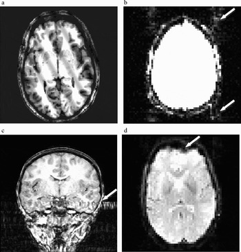
Noise, in the form of errant spikes in data intensity will appear as sine wave banding on the reconstructed image, and can vary in orientation and frequency. Because low frequencies in the data contain the majority of the image contrast, noise in this range results in low frequency, high contrast banding on the resulting image (see Figure 4a). High-frequency banding may be more difficult to detect because of its relatively low contrast. When looking through a data set, it is frequently easier to detect this type of noise by reducing image contrast and increasing image intensity. Depending on the cause of the spiking, the problem may be limited to only a single image, or may affect an entire data set. Spikes in the data frequently indicate a hardware problem and should be reported to the scanner technicians.

Figure 4.

Examples of image artifacts. (a) A T1-weighted image with sine wave banding due to noise spikes in k-space. (b) Ghosting (arrows) in an echo planar imaging (EPI) image. For purposes of illustration, the image intensity has been increased to highlight the presence of ghost images that are typically negligible. (c) A flow artifact (arrow) in a T1-weighted structural image. Note that the artifact extends through the temporal lobe as well as outside the head. (d) Geometric distortion and signal loss (arrow) in an EPI image, caused by air in the sinus at the front of the head.

Ghosting is a problem that may occur in fMRI data collected using EPI sequences, and refers to the presence of secondary images of the head that are shifted in space along the phase encoding direction (Smith, Reference Smith, Jezzard, Matthews and Smith2001; see Figure 4b). Ghost images are nearly always present in the data, but are usually of such low intensity that they are of no consequence. However, strong ghosting is cause for concern, and usually occurs for reasons that are beyond the control of the typical user. Therefore, the presence of ghosts may indicate a problem with the scanner that warrants the attention of the scanner technicians.

Flow artifact, which is primarily a problem with anatomical scans, is a result of distortion in the magnetic field that results from the rapid movement of protons in large blood vessels. One common source of flow artifact comes from the carotid arteries as they enter the base of the skull. This produces bands of distortion, similar to smearing, that extend into surrounding brain tissue, with the direction of the distortion depending on the direction of phase encoding (e.g., through the temporal lobes for left–right encoding; see Figure 4c). There is no way to correct for this type of distortion, so the experimenter must first run pilot subjects to determine the extent of the distortion present for their particular scanner and scan sequence, and decide which encoding direction produces the most acceptable results.

Participant motion can be problematic for both anatomical and functional data (Brammer, Reference Brammer, Jezzard, Matthews and Smith2001; Wood & Henkelman, Reference Wood and Henkelman1985). In the case of anatomical data, high-resolution images may require several minutes to collect data from the entire head. This is a long time for a participant to remain still. If head motion is relatively small, the resulting image slices will be only slightly misaligned. However, larger head motion across scan images can result in a badly misaligned three-dimensional representation of the brain. Head motion that occurs within a given slice appears as a blurring or image repetition that extends across the entire image in the phase encoding direction. Motion that results in differences in head position between slices will be evident as a staggering of image edges when the slices from a scan are stacked together to produce a three-dimensional representation of the data. Head motion can result in inaccuracies when making morphological measurements and can also result in difficulty accurately overlaying functional data onto anatomical structure. There is generally no way to correct for movement artifact that occurs in an anatomical data set.

Functional scans involve collecting data from multiple, relatively fast passes through the head, so that motion can be detected as differences in head position between subsequent brain volume images. Control of head motion is especially important in fMRI data because the signal changes due to the BOLD effect are small (Kwong et al., Reference Kwong, Belliveau, Chesler, Goldberg, Weisskoff and Poncelet1992). In contrast, changes in signal at a given spatial location that are due to head motion can be relatively large, overwhelming the changes in signal due to the hemodynamic response. After the data have been collected, mathematical algorithms can be used to track these shifts in position across time so that changes in participant position can be taken in to account during data analysis. However, it is important to remember that head motion inside the magnet results in brain tissue being scanned in different physical locations inside the magnetic field. As already discussed, the main field will have been shimmed with additional magnetic fields in an attempt to homogenize distortions in the main field due, in part, to the presence of the participant in the field. Once established, these shimming corrections are fixed. This means that if the participant moves significantly once a scan has begun, the signal from a given volume of tissue may no longer be collected at the same field strength, resulting in differences in signal that are not due to differences in activation, but to local main field strength. Thus, even with mathematical correction, participant movement introduces an unwanted source of variance into the fMRI data and should therefore be minimized to the extent possible.

Other sources of physiological noise, such as breathing and heartbeat, but also including movements such as swallowing or task-correlated head motion, are relevant in functional scans (Jezzard, Reference Jezzard, Moonen and Bandettini1999). Signal changes because of these types of physiological noise will overlay the signal changes due to functional brain response and may inadvertently confound the functional signal over time. To help counter this possibility, measures of heart rate and breathing rate can be taken while the participant is performing the behavioral task in the scanner. These data can then be used during data processing as confounding variables to remove the influence of these sources of physiological noise. However, the largest source of physiological noise may be subject motion that occurs in concert with some aspect of the behavioral task, such as the onset or offset of a given stimulus type. Signal changes produced by this motion will spuriously correlate with the functional changes in the BOLD signal, resulting in signal changes that appear to be a function of the behavioral task, but which are actually artifacts (Hajnal et al., Reference Hajnal, Myers, Oatridge, Schwieso, Young and Bydder1994). This makes control of head movement during functional imaging a critical component of any fMRI study.

Two other significant problems that are likely to occur with functional data are image distortion and signal loss, both of which are examples of artifact that occurs as a consequence of susceptibility (see Figure 4d). Susceptibility refers to the relative ease with which a given material becomes magnetized in the presence of an external magnetic field. Susceptibility artifact occurs when differences in the magnetic susceptibility of two adjacent substances result in a change in the local magnetic field that cannot be corrected by the shim gradients. This local inhomogeneity causes spin dephasing that results in loss of signal amplitude as well as spatial distortion in the resulting image. Distortion can appear as a stretching or compression of the image geometry, and the severity of the image distortion is a function of the inhomogeneities in the magnetic field, as well as the functional scan parameters. Fortunately, it is possible to mathematically correct offline for most inhomogeneities that are constant by using what is known as a field map. A field map is a separate scan sequence that measures inhomogeneities in the main magnetic field so that images collected in the field can later be corrected to compensate for these residual inhomogeneities (Jezzard & Balaban, Reference Jezzard and Balaban1995; Reber, Wong, Buxton, & Frank, Reference Reber, Wong, Buxton and Frank1998). Although most EPI data contain some distortion because of field inhomogeneities, many users do not correct for them using a field map because the distortions are not extreme. Other scan types (e.g., DTI sequences), however, may necessitate the use of a corrective field map because of the more extreme geometric distortions that result.

In contrast to field distortions where the data signal is compressed or stretched geometrically, susceptibility artifact that results in signal loss cannot be corrected. Signal loss is typically encountered at the juncture between tissue and an air cavity, such as a sinus. There is a large difference in susceptibility between paramagnetic substances, such as blood, and nonmagnetic substances, such as air, with little or no signal available from the nonmagnetic material. The combination of signal loss and geometric distortion can result in images that contain areas where brain tissue should be present, but which appear black, as though the air cavity were pushing into the brain. This phenomenon is variously known as signal loss, drop out, or blow out, and is commonly encountered in the prefrontal cortex near the sinus cavities at the front of the head, and in portions of the temporal lobe that lie above the air filled cavities of the ear canals. Although it may be possible to mathematically correct for the previously mentioned geometric distortion, any signal that has been lost because of susceptibility artifact cannot be recovered. A number of efforts have been employed to reduce signal drop out in specific imaging pulse sequences, including changes in slice orientation or alternate shimming techniques.

Preprocessing of functional data

After fMRI data have been collected and reviewed for any obvious artifacts, a number of important processing steps remain that may influence the quality of the data. Among these are intensity normalization, high-pass filtering, slice time correction, motion correction, spatial smoothing, coregistration, and spatial normalization. Although we discuss each briefly, the specific options available to the user will depend on the software used to process the data.

Intensity normalization refers to the adjustment of the intensity of each voxel in a functional volume of the head so that the overall intensity in the volume matches a particular value (e.g., the mean or median intensity across all volumes in the data set; Friston, Jezzard, & Turner, Reference Friston, Jezzard and Turner1994). This results in consistency of overall intensity across all of the volumes in an fMRI data series. High-pass temporal filtering removes variance that changes slowly over time and is therefore unlikely to be related to the behavioral task. It is also possible to apply a low-pass temporal filter to the data to remove variability that occurs on a time scale that is too fast to reflect signal changes because of the behavioral task. Although high-pass temporal filtering is fairly common, low-pass temporal filtering is less frequently encountered, and may be problematic in rapid event-related designs where the rapid presentation of different stimulus types may result in narrow peaks in signal that run the risk of being removed by a low-pass temporal filter.

Slice time correction involves mathematically adjusting the intensity values in a given functional brain volume to compensate for the fact that the volume image is not acquired instantaneously (Smith, Reference Smith, Jezzard, Matthews and Smith2001). In most functional scans, the brain volume is stimulated with an RF pulse and then data are collected from each slice in brain before the next RF pulse is applied and the next volume of data collected. This means that the data from each slice are collected not at a single point in time, but from across the entire scan TR. Even with a relatively short TR of 2 s, this means that the first and last slice in a given brain volume are collected at two different points in time. Nevertheless, subsequent data analysis operations assume that the data were collected at a single point in time. Slice time correction adjusts the volume voxel intensities to produce an estimate of the signal that would have occurred if all of the slices had been acquired at the same time, typically at the beginning of the TR.

Motion correction involves realigning each of the volumes in a functional data set to match the spatial positioning of a given volume (e.g., the first volume in the set; Cox, Reference Cox1996; Friston, Ashburner, et al., Reference Friston, Ashburner, Frith, Poline, Heather and Frackowiak1995). This is accomplished by estimating the difference in spatial location between voxels in adjacent volumes and keeping track of these differences from brain volume to brain volume through time. This is usually done for three degrees of linear translation and three degrees of rotation. Although large movements or movements that occur between functional runs can be difficult to correct, most current motion correction algorithms are very robust. In addition to realigning each volume in a series to a given volume, the estimates of movement can be included in the data analysis model as a confound variable to account for movement related variability in the fMRI signal.

Spatial smoothing, or spatial filtering, involves blurring the signal from adjacent voxels for the purpose of improving the signal/noise ratio. By blurring the signal across adjacent voxels, noise from each voxel is combined. Assuming that noise is random across voxels, local averaging will reduce the intensity of the noise. However, in order not to also reduce the intensity of the signal, it is important not to blur across an area wider than the functional activation of interest. It is generally not necessary to blur across a very wide area, and typical spatial filter values are on the order of two to three times the in-plane voxel size (spatial filter values of 4 to 6 mm are commonly encountered in the literature). In addition to increasing the signal/noise ratio for areas of sizeable activation, spatial smoothing has the additional advantage of decreasing the intensity of activation from very small areas of activation (e.g., single voxels) that may be spurious (Poline, Worsley, Evans, & Friston, Reference Poline, Worsley, Evans and Friston1997).

Coregistration involves aligning a set of functional data from a given participant to that participant's three-dimensional anatomical data. This is useful for overlaying statistical findings based on functional data analyses onto high-resolution anatomical images for the purpose of localizing areas of significant activation to specific brain regions. Because the morphology of the human brain varies widely between individuals it is first necessary to place individual functional data into a common physical space before pooling data from multiple participants. Such spatial normalization usually involves coregistering a participant's functional and anatomical data and then using the anatomical data to identify certain physical landmarks (e.g., the anterior and posterior commisures, as well as the edges of the brain surfaces; Woods, Grafton, Holmes, Cherry, & Mazziotta, Reference Woods, Grafton, Holmes, Cherry and Mazziotta1998a, Reference Woods, Grafton, Holmes, Cherry and Mazziotta1998b) that can be used as the basis for distorting the physical shape of the anatomical brain to fit a standard physical space (e.g., the Talairach atlas, Talaraich & Tourneaux, Reference Talairach and Tourneoux1988, or one of the Montreal Neurological Institute templates). Once the anatomical data have been transformed into the standardized space for a given participant, the same transformations can be applied to that participant's functional data. In this way, the functional data from multiple participants can be transformed into a standard physical space and pooled with a reasonable assumption that similar locations in space across participants correspond to similar locations in the brain. Note, however that numerous transformation algorithms exist, and that although the anatomical overlap between subjects for surface structures may be fairly good, the overlap across participants of deep structures in the brain (e.g., the hippocampus) may not be as good, depending on the particular algorithm used.

Analysis of functional data

The analysis of fMRI data usually involves the use of statistical methods that evaluate the fit of the hemodynamic response across time at each voxel to a number of predictor variables using a general linear model (Friston, Holmes, et al., Reference Friston, Holmes, Worsley, Poline, Frith and Fackowiak1995; Kutner, Nachtsheim, Neter, & Li, Reference Kutner, Nachtsheim, Neter and Li2005). The general linear model is a regression-based statistical model that allows the user to specify predictor variables for any number of behavioral conditions of interest, as well as control or baseline conditions and potential confounding variables such as subject motion. Any variability not explained by variables specified in the model is interpreted as unexplained, residual error. At each voxel in a given functional data set an estimate of fit is made for the different conditions and then t tests are performed to assess whether differences in fit between conditions, compared with baseline, reach statistical significance. In studies involving multiple participants this is typically done in two stages. The first stage involves fitting the model to each participant's data individually. Estimates of parameter fit from each participant are then subjected to a second stage of analysis that assesses whether differences between conditions within a group of participants are statistically reliable. Comparisons between different groups involve assessing whether the difference between conditions from within each group differs statistically (i.e., whether the difference of differences is significant). Thus, the inferences made using fMRI are always based on statistical assessments that compare one condition with another, typically with a baseline condition serving as the point of reference across conditions. Note that when comparing within or between groups of subjects, many MRI analysis programs do not assume, as a default setting, that subject is a random-effect variable. If the goal of the analysis is generalization to a representative population beyond the particular subjects who participated in the experiment, the researcher must make certain that subjects are being treated as a random-effect rather than a fixed-effect variable.

Because there is no absolute level of activation that is measured by the BOLD response, the measurements of signal change taken during one condition of an fMRI session are always interpreted relative to some other condition. This is most frequently a baseline condition thought to be unrelated to the experimental conditions of interest. The selection of an appropriate baseline is an especially important step in the experimental design process. Note that this is in contrast to some other neuroimaging methods, such as PET, in which the signal collected reflects the rate of metabolism in a given brain region. When significant differences between functional conditions are found, they are frequently displayed as pseudocolor statistical maps overlaid onto a representative coregistered anatomical image. It is important to understand that the fMRI pseudocolor illustrations presented in journal articles are representations of the result of statistical comparisons between experimental conditions. That is, they are color-coded maps showing the results of statistical tests (typically t tests) at each voxel in the image and do not represent differences in magnitude of activation. It is easy to misinterpret “hot spots” in such images as showing large magnitude differences between conditions, when in fact they simply indicate highly significant differences between conditions. For example, highly significant differences may reflect either large or small differences in magnitude (e.g., small differences between conditions in the presence of small variability). Conversely, low significance or subthreshold differences may also reflect either small or large differences in magnitude (e.g., large differences between conditions in the presence of large variability). Thus, just as with the interpretation of results from behavioral analyses, one must remember to interpret significant differences presented in pseudocolor MRI images by examining differences between factor levels in the analysis.

Among the many complications involved in the statistical analysis of fMRI data is the fact that whole-brain analyses involve making comparisons between conditions of interest at every voxel in the brain. For a typical adult brain scanned at a voxel resolution of 1 mm³, this may mean as many as 100,000 t tests are performed for each statistical comparison, raising the likelihood that a large number of spuriously significant voxels will be detected (Loring et al., Reference Loring, Meador, Allison, Pillai, Lavin and Lee2002). To correct for this likelihood, a number of correction methods have been devised including the application of statistical techniques, such as the Bonferroni or the false discovery rate (Benjamini & Hochberg, Reference Benjamini and Hochberg1995; Genovese, Lazar, & Nichols, Reference Genovese, Lazar and Nichols2002) correction methods, or the application of random field theory (Lange, Reference Lange1996; Worsley, Marrett, Neelin, & Evans, Reference Worsley, Marrett, Neelin and Evans1992). Many researchers, however, opt to constrain false positives by choosing a more stringent p value (e.g., p = .005) and/or requiring that a cluster of adjacent voxels surpass a certain total volume before it is declared meaningfully significant. Both of these methods serve to prevent spuriously occurring, suprathreshold voxels from being considered meaningfully related to the task conditions. The choice of method may depend on the software being used for statistical analysis, as well as the opinions of the researcher regarding the most appropriate method for controlling false positives. This is an area of ongoing research in the analysis of functional imaging data.

One final consideration in the analysis of fMRI data that is related to the issue of controlling for multiple comparisons is whether to perform statistical analysis across the whole brain or whether to limit analysis to specific regions of the brain. The latter approach is known as region of interest (ROI) analysis, and can help control for multiple comparisons by reducing the number of voxels that are subjected to statistical analysis (Constable et al., Reference Constable, Skudlarski, Mencl, Pugh, Fulbright and Lacadie1996). ROIs may be defined a priori or may be functionally identified. ROIs that are defined a priori might, for example, target specific brain structures or networks hypothesized to show differential involvement for different behavioral conditions. In contrast, functional identification of ROIs is essentially a post hoc analysis involving two stages. First, a whole-brain, voxelwise analysis is used to identify brain areas that show robust differences between conditions. Then, after functional regions of interest have been identified, subsequent analyses are restricted to these local ROIs. In both cases, ROI analyses are typically conducted using a mean representation of the signal from a given ROI, rather than on a voxel by voxel basis. Although functional identification of ROIs is a commonly employed technique, it is clearly an exploratory method, and is thus less theoretically rigorous than a priori identification of ROIs.

Scanner acclimation

The physical appearance and noise of a typical scanner can seem intimidating to anyone. However, to a child or to someone with a heightened state of anxiety, these aspects of the scanning session may be especially overwhelming. Even for participants who demonstrate enthusiasm during the explanation of the experimental session, being in the presence of the scanner can sometimes elicit feelings of anxiety and uncertainty. To lower both attrition rates and the anxiety levels of those participants who enter the scanner, acclimation to the scanner environment through the use of a simulated scanner experience can be essential (Rosenberg et al., Reference Rosenberg, Sweeney, Gillen, Kim, Varanelli and O'Hearn1997; Thomas & Casey, Reference Thomas, Casey, Moonen and Bandettini1999). Ideally, this might involve the use of a mock scanner that closely replicates the sights, sounds, and feel of the actual scanner itself. This will provide the participant with the opportunity to explore the novel physical environment and to become accustomed to the experience of lying supine in a tunnel-like apparatus, while at the same time giving the experimenter an opportunity to assess the participant's comfort level and the likelihood of claustrophobia. If a realistic replication of the scanner is not feasible, even a relatively crude facsimile of the scanner bore, such as a plastic play tunnel, along with audio presentation of the scanner sounds, will provide children with a better sense of the actual scan experience than can be provided by verbal description alone.

In addition to familiarizing the participant with the physical scanner environment, a simulated scanner experience can increase the likelihood that the participant will yield good-quality behavioral data, as well as motion-free functional imaging data. While in the scanner simulator, practice sessions can be administered to help familiarize the participant with the requirements of the behavioral task. This technique gives the experimenter an opportunity to explain the task in the context in which it will actually take place, and gives the participant the opportunity to learn to perform the task in the unusual position of lying on his/her back in a tunnel. This latter point is important because many participants do not realize that they will be unable to look at their hands when making a manual response. This is especially important when dealing with young children, as the unconscious tendency to look at the hands when responding is quite strong in young participants. In addition, many scanners present visual stimuli through the use of a periscope-style mirror system and record manual button presses through the use of response pads attached to one or both hands. Comfort with both of these aspects of the experimental session is critical to the acquisition of good behavioral data. A short familiarization session in the scanner simulator also allows the experimenter to give feedback to the participant regarding movement. Even when asked to remain still, children (and many adults) have a tendency to fidget when they are lying down for extended periods of time. Careful observation of participant movement in the simulator permits the experimenter to make the participant more aware of their movements, and can alert the experimenter that a particular participant may require greater vigilance regarding motion when the actual scan takes place. For populations that may be especially prone to movement, such as children or certain behavioral groups, the simulator may also provide an opportunity to present a training routine to help limit participant motion (e.g., the use of a tracking system to turn off a video display whenever the participant's head moves beyond a certain criterion; Thulborn, Reference Thulborn1999).

Motion reduction

Even if participants take part in a scanner simulation, it can be very difficult to remain motion free for long periods of time during an actual scanning session. To reduce motion inside the scanner, most researchers employ some type of physical restraint mechanism on the head. These include bite bars, semiflexible face masks, and head-conforming foam or pillows. With children and patient populations, the more physically restrictive of these options, such as bite bars or face masks, may actually increase participant discomfort and anxiety, making it less likely that they will complete a scanning session. We have found that reasonable constraints on head motion can be achieved through the use of a plastic bag filled with head-conforming styrofoam beads. The bag is placed beneath the participant's head and neck and wrapped up on either side of the head. Because of its extreme flexibility the bag can even fit around the headphones used during the scan. Excess air is then evacuated from the bag, which causes the styrofoam beads in the bag to become fixed in position. This forms a semirigid shell around the participant's head that helps keep the head in a fixed position, but that also provides tactile feedback when the participant moves. With special populations, the use of some form of head restraint is highly recommended.

Design considerations for functional studies

When planning an fMRI experiment there are a number of factors that must be taken into consideration in addition to the particular sequence parameters to be used at the scanner. These involve the establishment of a research paradigm that will accommodate the nature and limitations of the BOLD response as well as the research questions of the experimenter. When investigating pediatric and atypical populations, there are two ways in which one might think about this. The first is in the formation of specific hypotheses regarding functional differences that would be expected with behavioral performance, across different age groups, or between typically and atypically developing groups. The second is in the creation of task conditions that tap the relevant brain systems that underlie cognitive behaviors. This includes the establishment of a suitable baseline condition against which to compare the functional response to behavioral conditions of interest.

Given the complexities of fMRI data collection and analysis, it simply is not sufficient to run two groups in an experimental paradigm and note functional differences between groups in the absence of constraining hypotheses. This is especially true if the groups are likely to differ in brain morphology and/or function as a consequence of differences in developmental stage or pathology (physical or behavioral). Prior behavioral, physiological, or pharmacological research suggesting differences or deficits in the function of specific brain regions or systems between groups offers the best starting point for a successful fMRI study. Having identified a target brain system that one hypothesizes to differ in function between groups of interest, the experimenter's task is to design a behavioral paradigm that will successfully tap that functional difference.

Although it can be tempting to transfer behavioral tasks that have been used outside the scanner environment directly into the context of fMRI, this must be done with care (Casey et al., Reference Casey, Trainor, Orendi, Schubert, Nystrom and Giedd1997). A number of methodological issues are at stake that may influence the outcome of the fMRI experiment. First is whether the transition to the scanner environment will influence participant behavior. For passive perceptual tasks this may not be a significant problem, but on tasks that require the participant to provide contingency-based responses (e.g., where behavioral performance between conditions is indexed by accuracy or reaction time) there is frequently a reduction in performance associated with performing the task in the scanner (Thomas et al., Reference Thomas, King, Franzen, Welsh, Berkowitz, Noll, Birmaher and Casey1999). This phenomenon tends to be exacerbated in pediatric and patient populations. Pilot data may be needed to ensure that similar behavioral differences between experimental conditions are found both in and out of the scanner. Conversely, for behavioral conditions that have never been tested with a particular population, it is advisable to collect a set of behavioral data outside the context of the MRI scanner prior to undertaking the expense of collecting fMRI data.

Two other very important issues are whether the experiment will involve a block design or an event-related design, and whether stimulus presentation will be participant driven or yoked to the scan TR. These decisions may depend on the nature of the task. For example, it would be difficult to administer an oddball task using a block design. However, where appropriate, block designs tend to yield greater power because the signal measured during each block is at saturation. Event-related designs tend to have trials yoked to some multiple of the scan TR (although trial onsets may be jittered), rather than allowing trial progression to be participant driven. This facilitates the allocation of different scan volumes to different behavioral conditions. In contrast, block designs are better able to accommodate participant driven stimulus presentation because there is no need to associate individual scan volumes (MR data points) with the onset of individual stimuli within the block. An additional concern regarding event-related TR-yoked designs is the use of experimental paradigms that involve rapid responses followed by several seconds of delay before the onset of the next stimulus. Consider, for example, collecting event-related data with a TR of 2 s in which trials occur once every 4 s. If the subject responds within the first second, the remaining 3 s of the trial involve uncontrolled cognitive activity. Presumably, this activity will vary across the duration of a given participant's scan and will also differ between participants. However, in such situations, one must be careful that the experimental stimuli or experimental context do not bias participants to have unintended consistencies between conditions during these periods of uncontrolled activity.

In designing an fMRI experiment, the choice of an appropriate baseline condition is crucial to the interpretation of the results (Stark & Squire, Reference Stark and Squire2001). Recall that MRI functional activation to conditions of interest must be analyzed against other conditions, because the MRI signal does not reflect an absolute measure of neural activity. Although it is possible to contrast activations between conditions directly, one usually wants to establish a baseline task to help isolate activity that is specifically related to the cognitive function under investigation. Toward that end, the choice of a baseline task can strongly influence the interpretation of the data. For example, if one is investigating brain function associated with visual search during conditions of active search versus visual pop-out, the ability to assess brain areas involved in these two conditions (as opposed to differences between these conditions) requires the use of a baseline condition against which to compare activation from each condition separately. Very different patterns of activation may be revealed for a given condition depending on whether the baseline is, for example, a blank screen with a fixation point, or a field of “special” visual objects that mimics the visual properties of the conditions of interest but which the participant knows need not be searched. The choice of baseline will determine, in part, what aspects of the cognitive task are reflected in the resulting analysis output. If a fixation point is used as baseline, the contrast between visual search conditions and baseline will reflect not only search related activity, but also activation related to differences in low-level perception. In contrast, a baseline condition involving a “special” pseudosearch field will presumably elicit much of the same type of low-level perceptual activation as the search conditions. Thus, the difference between the pseudosearch baseline and search conditions will reflect differences in activity that are more closely related to visual search per se. This step in the fMRI experimental design process requires careful consideration, especially as it may be novel for many experimenters.

Investigations involving pediatric or clinical populations must take into account a number of special concerns related to within- and between-group variability that are less prominent in studies involving only typically developing adults. Data collected from special populations may show relatively high levels of within-group variability that can contribute to apparent functional differences between groups. It is the responsibility of the researcher to determine if such differences are meaningful or spurious. There are three primary sources of this type of variability. The first involves gross differences in the size of various brain structures that may occur across development or as a consequence of pathology (Castellanos, Giedd, Hamburger, Marsh, & Rapoport, Reference Castellanos, Giedd, Hamburger, Marsh and Rapoport1996; Giedd et al., Reference Giedd, Vaituzis, Hamburger, Lange, Rajapakse and Kaysen1996). Because of this, one must be cautious when making comparisons that involve functional data from special populations that have been transformed to fit the brain space of a typical adult population. The mathematical algorithms that perform this kind of transformation do so without consideration of whether the end result produces comparable colocalization of many brain structures. Functional comparisons between groups that differ in the size and/or location of target brain structures may lead to group differences that have more to do with differences in morphology than functional activation. In cases where large differences in brain morphology appear between groups (e.g., in certain neurological populations), it may be more reasonable to use analyses that compare mean signal change in regions of interest between groups, rather than to perform analyses on a voxel by voxel basis.

Differences in signal variability may also be a concern in fMRI experiments, not only for comparisons between groups, but also for comparisons within groups (Thomas & Casey, Reference Thomas, Casey, Haan and Johnson2003). A number of relevant factors, including cellular and vascular organization, are likely to differ at various stages of development and may vary with psychopathology. Thus, variability in the MR signal, independent of additional confounding factors such as morphological differences or increased motion, is likely to be greater in pediatric and patient groups than in healthy adults. This raises the possibility that, to obtain equivalent statistical power within a special population, one may need a larger sample size than would be required to detect a statistically reliable difference in a typically developing adult population. Just as is the case with analyses of behavioral data, estimates of power and effect size are needed to determine appropriate sample sizes.

It is important to note that experimental groups may show differences not only in the intensity of significant differences between conditions, but may also show differences in the volume of cortex over which these differences occur (Durston et al., Reference Durston, Davidson, Tottenham, Galvan, Spicer, Fossella and Casey2006). This is especially the case for younger age groups. Unfortunately, however, the interpretation of differences between groups can be problematic, as such differences may reflect differences in the maturational or physiological organization of the brain, differences in cognitive strategy employed to accomplish a particular behavioral task, or differences in some other factor, such as global levels of anxiety (Thomas & Casey, Reference Thomas, Casey, Moonen and Bandettini1999). Care must be taken to tease apart these potential sources of difference. Fortunately, some potential confounds such as anxiety level can be independently assessed at the time of scan. Measures of heart rate and respiration can be obtained throughout the scan, or even outside the scanner, pre- and postscanning. Such measurements can help identify individuals whose physiological anxiety indices are outside an acceptable range. It is also possible to use subjective measures of anxiety, such as selfreport, although this may not be feasible with some populations, including the very young.

Within-group correlations between functional activation and behavioral performance can help establish more substantive links between behavior and brain activity (e.g., Casey et al., Reference Casey, Trainor, Orendi, Schubert, Nystrom and Giedd1997; Thomas et al., Reference Thomas, Drevets, Dahl, Ryan, Birmaher, Eccard, Axelson, Whalen and Casey2001). Clearly, it is difficult to interpret differences in brain activity if large differences in behavior are also present. Within-group correlations between behavior and activity can help overcome this difference in behavioral performance if similar trends in correlation are found. More ideally, however, would be a situation in which behavioral performance between groups was equated. In such a case, differences in brain activation may be more easily understood in terms of differential recruitment of brain areas and/or differential levels of activation within a given area in the service of equivalent performance. It may be possible to design some experimental tasks to equate differences in behavioral performance, for example, by running pilot studies to determine experimental parameters that produce equivalent performance between groups. Alternatively, one could design a study that parametrically manipulates critical factors to produce a range of behavioral performance within each group (e.g., Braver et al., Reference Braver, Cohen, Nystrom, Jonides, Smith and Noll1997; Durston, Thomas, Worden, Yang, & Casey, Reference Durston, Thomas, Worden, Yang and Casey2002), which can then be selected for behavioral equivalence post hoc. This latter strategy, however, would be relatively inefficient if only a small portion of the collected data is used for analysis. Instead, an optimal strategy would be to design a parametric manipulation that permitted assessment of differences in brain function between groups when equated for performance, as well as an assessment of changes in brain function that may occur within the group as a function of the parametric manipulation (Casey et al., Reference Casey, Forman, Franzen, Berkowitz, Braver and Nystrom2001; Durston et al., Reference Durston, Tottenham, Thomas, Davidson, Eigsti and Yang2003).

Finally, although it will be obvious to many readers, the study of developmental psychopathology is even more challenging than the study of typical development. Developmental psychopathology involves the added complexities of timing of symptom onset and pluripotentiality of developmental trajectory following onset. Therefore, characterizing the nature of a given disorder requires not only the comparison of typical and atypical groups, but also the investigation of the range of variability that occurs within the disorder. This applies to both the design of tasks that will be used in fMRI studies as well as the interpretation of the resulting data. The study of psychopathology can be especially difficult given that typical brain development, both anatomical and functional, has not been well characterized in many domains of interest.