Experimental design

This experiment was approved by the University of New England Animal Ethics Committee (AEC 14/002). Angus cattle lines divergently selected for low or high residual feed intake (RFI) established at the Trangie Agricultural Research Center, New South Wales, Australia (Arthur et al., Reference Arthur, Herd, Wright, Xu, Dibley and Richardson1996 and 2001) provided 20-month old steers (n = 30) and heifers (n = 34) of starting live weight 406.9 kg (±35.8 SD) generated by ~2.5 generations of divergent selection. Steers and heifers were allocated in two separate feedlot pens. Three heifers and one steer were removed from the study before measurements commenced due to initial inappetence, so that 29 steers and 31 heifers were available for RFI and potentially for methane emission measurement. The total duration of the test (excluding the induction to the feedlot ration) was 70 days and heifers and steers were swapped between pens on day 35. A total of 24 animals having the most methane data (>85 or more measures of >3 min length) were chosen from these 64 animals for intensive study of the effects of feeding pattern on DMP (17 heifers and seven steers; nine high RFI and 15 low RFI genetic merit animals).

Animals and feeding

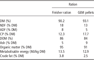
Over 14 days cattle were adjusted to a total mixed ration (TMR) based on barley, cottonseed and hay (Table 1) provided for ad libitum consumption, with the ration being dispensed through GrowSafe automatic feeders (GrowSafe Systems Ltd., Airdrie, AB, Canada). Each pen had four individual automatic feeders, enough to provide ad libitum feeding for the animals’ BW (Bindon, Reference Bindon2001). These feeders recorded the number of feeding events and the duration and weight of feed consumed at each feeding session (called a ‘feed event’) and were activated by radio-frequency identification (RFID) whenever an animal entered the feeding stall. A meal was defined as the period from which a new animal was detected in the automatic feeder and continued until the animal left. Weekly subsamples of the feed were frozen and pooled for later analysis of nutrient content (Table 1). Chemical analysis of the feed was conducted by Wagga Wagga Agricultural Institute (New South Wales Department of Primary Industries, Australia).

Table 1

Chemical analysis of the finisher feedlot ration fed to steers and heifers during the experimental period as their main ration and as supplement pellets supplied by the GEM unit

GEM = GreenFeed emission monitoring; DM = dry matter; DOM = digestible organic matter.

Finisher ration composed of barley (73%), cottonseed (10%), hay (8%), liquid supplement (5%), water (4%) as mixed.

Methane measurements

DMP was estimated from multiple short-term breath measurements using the GEM (manufactured by C-Lock Inc., Rapid City, SD, USA). The GEM is a feeding station where pelleted supplement is provided to cattle in a controlled manner (quantity/feed event and number of feed events/day) based on their identity detected by an RFID ear-tag. To access the supplement, cattle placed their head in an open shroud into which pellets are dispensed from a hopper. Air was continuously drawn through the shroud and past the neck of the feeding animal at a precisely measured rate. The concentrations of CH₄ and CO₂ were measured in the exhaust gas. Background gas concentrations were measured when no cattle were present and periodic calibrations and recovery tests performed to define sensor responses to known concentrations of methane and CO₂ and to ensure that >96% of the CO₂ test gas released into the GEM shroud was recovered in the exhaust gas stream. A spot measurement period of 3 to 5 min typically detected several eructation events and is called a ‘spot sample’ hereafter. To avoid data when animals stepped away from the shroud during methane measurement, a proximity sensor in the shroud, that monitors head-position of the animal throughout each feeding event, was used to identify this happening with such data being excluded. The emission rates over all useful feeding events (at least 3 min length with head in position) during a day were averaged to provide a mean DMP for that day. The pellets delivered in the GEM unit were 6 mm in diameter and the system was programmed to deliver up to four drops, each of 53 g DM, separated by 45 s and then wait at least 3 h to allow a new supplement session for an individual animal. GEM pellets were formulated to closely match the ingredients and nutrient content of the main diet (Table 1) and also contained 0.075% aniseed XL flavoring (Fluidarom 1957, Norel Spain) to increase pellet palatability.

Data processing

The data from the GrowSafe feeders and GEM units were transferred to an Excel spreadsheet with the following columns: tag number, pen/GEM unit, date and time of feed event, length of feed event, CO₂ (g/day), CH₄ (g/day) and TMR intake (g). The GEM emission data were interspersed with GrowSafe feeder data, with data rows arranged in chronological order for each animal. Visual basic (VB) routines were written to calculate the time interval before each spot methane measurement and each recent feed event and then associated with the amount eaten at each feed event. The VB code calculated the time intervals and meal size of all feed events for up to 3 days before each spot methane measurement. The maximum number of feed events in the 3 days before a GEM spot measurement for any animal was 71. Methane measurements within the first 3 days of feeding the finisher ration were omitted from the analyses.

Data analysis

Relationships between spot emission rate and intake were studied using different approaches reliant on increasing levels of feed information inputs as described below.

GLM

Daily intakes, measured DMP and MY were plotted over the entire feeding period revealing notable patterns over time in each trait. For each measured DMP, the average daily intake for the 3 previous days was used to calculate MY. Splines over time (with 3 DF) were fitted for the diurnal effect and days. Animals were fitted either as random effects, or as a fixed effect and the interaction estimated (i.e. allowing the animals to have different patterns over time). The predicted DMP and MY values for the animals were also estimated using the equations used in the Australian National Greenhouse Gas Inventory Report for feedlot beef cattle (Department of Environment, Reference Dijkstra, France, Dhanoa, Maas, Hanigan, Rook and Beever2014; Moe and Tyrell, Reference Moe and Tyrrell1979). Concentrations of lignin (1.1%) and silica (0.1%) were assumed in estimating the cellulose content in the diet (cellulose = ADF−lignin−silica) to solve the Moe and Tyrell (Reference Moe and Tyrrell1979) equation.

Raw data, feed events and diurnal variation in emissions

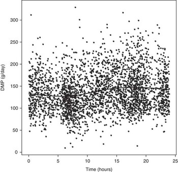
There were 18 700 rows of raw data, being individual methane production measures of 24 cattle over 64 days during the 70 days test. The number of feed events in the 3 days before a methane measurement was normally distributed with a mean of 32±9.6 (median 31, mode 33) and a range from 8 to 71. As meal frequency increased the average size of each meal diminished from 1228 g (±1006) at the first meal in the 3 days before each methane measurement to 190 g (±180) for the 71st meal in the preceding 3 days for the animals with 71 feeds. For DMP, day (as a spline term) was the dominant effect, with R ² of 23.3%. The diurnal effect (Figure 1) lifted this to 27.7%, and then adding ‘animal’ as a fixed effect gave a final R ² of 36.1%.

Figure 1

Diurnal spline fit for DMP based on spot emission rates of methane for 24 Angus cattle on a feedlot total mixed ration. DMP = daily methane production.

Curve fitting

Simpler models

The simple models of spot DMP v. time since the most recent feed event explained little variance in spot DMP, reflecting the high variability in spot measures and that these models did not include the size of the feed event or time and size of earlier feed events. For example, the R ² of the one-compartment dose model varied from 0.01 to 0.23 for the 24 cattle, averaging 0.10. Daily intake is recognised as a good predictor of DMP (Kennedy and Charmley, Reference Kennedy and Charmley2012), but association of spot emission rate with the most recent feed event or events was poor.

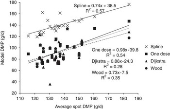
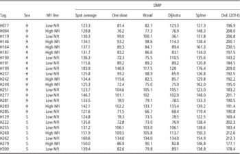
When the arithmetic mean spot emission rate for the trial for each animal was regressed against the fitted DMP, estimated as the area under the curve from models relating emission rate to time since last feed, the proportion of average spot rate variance explained (Figure 2), was R ² = 0.54 for the one dose curve fit. The estimated areas under the curves equating to average DMP for the time curves are given in Table 2.

Figure 2

Estimates of DMP based on the integrated areas under curves derived from four models plotted relative to the average spot emission from each of the 24 Angus cattle over 64 days on a feedlot total mixed ration. DMP = daily methane production.

Table 2

Estimated daily methane production (DMP: g/d) calculated as the arithmetic mean of all individual measurements (spot average) for individual cattle on feedlot rations (tag) or derived from the areas under various curves or as predicted by DoE (Reference Dijkstra, France, Dhanoa, Maas, Hanigan, Rook and Beever2014) equations

DMP = daily methane production; NFI = net feed intake; H = heifer; S = steer.

The spot average (and spline) DMP estimates were lower and dissimilar to DoE (Reference Dijkstra, France, Dhanoa, Maas, Hanigan, Rook and Beever2014) estimates, which use Moe and Tyrell’s (Reference Moe and Tyrrell1979) equation, and are the basis of Australia’s Greenhouse Gas Inventory reporting. However, DoE (Reference Dijkstra, France, Dhanoa, Maas, Hanigan, Rook and Beever2014) estimates appear too high (e.g. Benchaar et al., Reference Benchaar, Rivest, Pomar and Chiquette1998) and therefore are of limited use as a benchmark DMP value. The correlations of DoE (Reference Dijkstra, France, Dhanoa, Maas, Hanigan, Rook and Beever2014) estimates of DMP to the spot average, one dose, Wood, Djikstra and spline models were 0.29, 0.37, 0.31, 0.02 and 0.52, respectively. The correlations between the average of spot estimates of methane and the curve estimates in Table 2 are shown in Figure 2. The spot average was more highly correlated to areas under fitted curves than to DoE (Reference Dijkstra, France, Dhanoa, Maas, Hanigan, Rook and Beever2014) estimates but the values were about 40 g/day higher than estimated from the areas under the various curves. The one-compartment dose model using only time since the immediately preceding feed event fitted the data in this study better than the two intake quadratic model and had the highest correlation to the average spot estimates (r = 0.74). This was the model therefore used for additional analyses.

Three-day intake models

Solver was used to fit ‘the average’ (across-animals) one-dose model to DMP, scaled to a 1 kg feed event (so the feed amount was factored in and directly scaled). MY was the integral under this curve and was very close to the ‘average’ (on a per-animal per-day basis) estimated MY values.

The variation in the DMP data resulted in a fitted model in which only 16.9% of variation was explained by modelling GEM spot measurements in relation to the size of, and interval from, each meal in the previous 3 days. The fitted model allowed a lag period (from time of intake to start of methane production), but this always fitted as zero and rise to peak emissions was very rapid. Supplementary Figure S1 shows the instantaneous emission rate over time for ‘the average animal’ for 3 days, following a 1 kg feed event. The integral under this MY curve was 12.1 g/kg DMI.

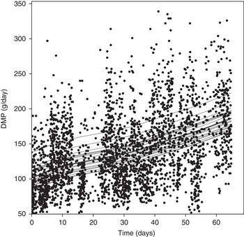
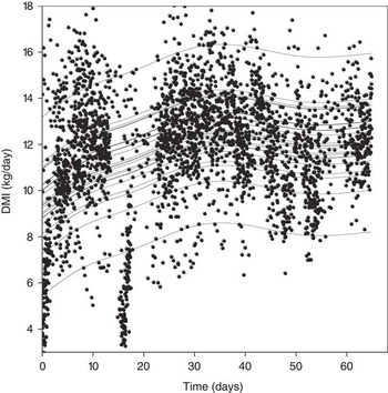
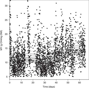
This model identified marked animal differences about the mean MY value of 12.1, where MY was calculated as the ratio of DMP on a given day and the average DMI on that day and the previous 2 days. To better understand the changes in emission attributes over time, DMI, DMP and MY over the trial were plotted and splines were fitted. The R ² for DMP fitted by splines was 24.1%, and Figure 3 shows steady increases in DMP calculated from spot measurements over time, which were consistent between animals. The average DMP values were 101.1 g/day at day 0, 136.4 g/day at day 30 and 190.1 g/day at day 65, so DMP increases were 1.53 g/d from days 30 to 65, or 1.37 g/d for the whole trial. This trend in increasing calculated DMP with time was mostly due to changes in daily intake over time, with the same spline model for DMI having R ² of 41.1%, as shown in Figure 4. Taking the ratio of DMP on a given day and DMI (averaged over day of measurement and 2 previous days) to calculate MY, the same model gave an R ² of 18.1%, as shown in Figure 5.

Figure 3

The fitted spines for estimated DMP of individual beef cattle (n = 24) on a feedlot total mixed ration with splines for individual animals. DMP = daily methane production.

Figure 4

The fitted spines for estimated DMI of individual beef cattle animals (n = 24) on a feedlot total mixed ration with splines for individual animals. DMI = dry matter intake.

Figure 5

The fitted splines for estimated MY for individual beef cattle (n = 24) on a feedlot total mixed ration with splines for individual animals. MY = methane yield; DMI = dry matter intake.

MY was steady until around day 40. MY for the first 37 days averaged 11.5 g/kg DMI; for the last 26 days it showed a steady increase, with an average of 13.9 g/kg DMI. There was the same degree of between-animal variability as was noted with the 3-day model (a few animals had very high MY values). While these MY values are lower than other studies (e.g. Ramin and Huhtanen, 2013) they match observed data (MY 13.6 g/kg DMI) for similar concentrate diets (Hegarty et al., Reference Hegarty, Goopy, Herd and McCorkell2007) and with these same 24 animals measured in respiration chambers on the same diet (MY 15.5 g/kg DMI; Herd et al., unpublished data) 2 months later. The accuracy of using GEM has been shown (Velazco et al., Reference Velazco, Cottle and Hegarty2014) through comparison with respiration chambers, so there is no reason to doubt the accuracy of the GEM as the CO₂ recoveries were high (95.9% and 97.9% of the gravimetrically determined quantities of CO₂ released into the shroud were recovered by the two GEM units used in the experiment). All model methane estimates and the average of spot estimates were lower than those predicted for feedlot cattle using Moe and Tyrell (Reference Moe and Tyrrell1979). As noted previously, the equation of Moe and Tyrell (Reference Moe and Tyrrell1979) has been shown to have a very high error of prediction, a high general bias and explain a relatively low proportion of variance in methane production (Benchaar et al., Reference Benchaar, Rivest, Pomar and Chiquette1998; Ellis et al., Reference Ellis, Kebreab, Odongo, McBride, Okine and France2007).

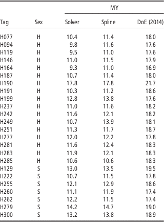
A comparison of the solver, average spline and DoE (Reference Dijkstra, France, Dhanoa, Maas, Hanigan, Rook and Beever2014) estimates of MY for each animal are shown in Table 3. The correlation between solver and spline MY estimates was 0.91 and with DoE (Reference Dijkstra, France, Dhanoa, Maas, Hanigan, Rook and Beever2014) MY estimates was 0.83. The correlation of spline and DoE (Reference Dijkstra, France, Dhanoa, Maas, Hanigan, Rook and Beever2014) MY estimates was slightly lower at 0.78.

Table 3

Average methane yield (g CH₄/kg DM intake) of beef cattle on feedlot rations estimated by solver, splines and DoE (Reference Dijkstra, France, Dhanoa, Maas, Hanigan, Rook and Beever2014) equations

DM = dry matter; MY = methane yield; H = heifer; S = steer.

Power analysis

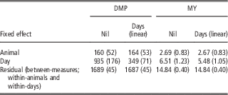
The precision of estimated DMP or MY values, with or without available feed intake data, depends on the inter-play between the different sources of variation and the numbers of replicates within each component. Taking our DMP estimate based on spot emission data as an example, we first fitted a ‘base’ mixed model with no fixed effects and ‘animals’ and ‘days’ as the random effects (to estimate their variance components). As listed in Table 4, the residual variances were large (v. their respective standard errors). As shown previously (Figure 4), however, ‘days’ do not appear to be a simple random effect, as there is an increasing trend in DMP over time. Table 4 also shows the variances for a second mixed model where the observed trend is accounted for by including a linear term as the fixed effect.

Table 4

Variance components (SE) from the GLM models of DMP (g CH₄/day) and MY (g CH₄/kg DM intake) of beef cattle on feedlot rations

DMP = daily methane production; MY = methane yield; DM = dry matter.

Residual variance includes variance components other than between-animal and between-day variances.

Removing the trend in days reduced the estimated variance components for days from 935 to 349 for DMP and 6.5 to 5.5 for MY. Even when de-trended, the variance components for days are notably larger than those for animal. Other cattle methane studies (e.g. Blaxter and Clapperton, Reference Blaxter and Clapperton1965; Boadi et al., Reference Boadi, Wittenberg and Kennedy2002; Harper et al. Reference Harper, Denmead, Freney and Byers1999; Pinares-Patino et al., Reference Pinares-Patiño, Baumont and Martin2003; Vlaming et al., Reference Vlaming, Lopez-Villalobos, Brookes, Hoskin and Clark2008) indicate that between-day variance in DMP is more likely to be closer to our lower value (i.e. when the effect of our linear trend is removed), so we used the between-day variance value of 349, rounded to 350, in a power analysis of experimental designs for DMP estimated from spot measurements.

For the power analyses of DMP, we rounded the linear trend values to 1700 for the residual variation and 160 for the variance components for animals. The power analysis investigated the precision of the estimated mean using the 95% two-tailed confidence interval, taking the variance formulae in Cox and Solomon (Reference Cox and Solomon2003) as shown below:

$${\rm SE}\,{\rm (mean)}\!{\equals}\sqrt {{\rm [}\sigma ^{{\rm 2}} (n_{a} {\times}n_{d} {\times}n_{r} ){\plus}\tau _{a} \,/\,n_{a} {\plus}\tau _{d} \,/\,n_{d} {\rm ]}} {\rm }$$

where σ ² is the residual variance, n _a , n _d and n _r , respectively, the numbers of animals, days and replicates and τ _a and τ _d the variance components for animals and days, respectively.

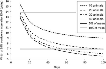
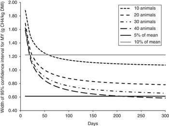
The targeted precision was 5% of the estimated 64 days mean DMP or MY. Hence, we expect 95% power for any future experiments with combinations of numbers of animals, days and replicates where this target is met. Figures 6 and 7 show these patterns for DMP and MY, respectively, assuming two spot measures are made per-animal per-day (as occurred in this study).

Figure 6

Estimated width of 95% confidence intervals (either side of mean) for DMP of beef cattle v. numbers of days for different numbers of animals (dashed lines) and the targeted 5% or 10% of the observed mean (solid black and grey lines, respectively). Two spot measures of methane production rate per day are assumed. DMP = daily methane production.

Figure 7

Estimated width of 95% confidence intervals (either side of mean) for daily MY v. numbers of days, for different numbers of beef cattle (dashed lines) and the targeted 5% or 10% of the observed mean (solid black and grey lines, respectively). Two spot measures of methane production rate per day are assumed. MY = methane yield; DMI = dry matter intake.

As shown in Figure 6 it is realistically infeasible to achieve the targeted precision for DMP from a population of only 10 animals. With 20 animals 98 measurement days are needed. Doubling the number of animals to 40 results in 47 days being required (a time reduction of 52%). Conversely, for a 50-day trial 36 animals are needed to achieve the targeted precision; v. 20 animals for a 100-day trial (a 44% reduction in the number of animals). So while the between-day variation was higher than between animals, the overall differences in the required numbers of days or animals are not all that pronounced, so the numbers of animals and days are reasonably interchangeable in respect to power of the test. They both contribute equally to reducing the residual variance. The design of each future experiment will, of course, depend on the available budget and logistic limitations, but our formula and figures can be used as a guide for experimental design.

The maximum number of spot measures per-animal per-day (n _r ) is set by the researcher but whether cattle utilise all the measuring opportunities is the animal’s choice. However, increasing n _r only had a relatively minor effect here – for 20 animals, the required number of days to achieve target precision only reduces from 98 (for n _r = 2) to 91 for n _r = 5 and to 89 for n _r = 10. For 40 animals, the required numbers of days were 47, 45 and 44 for n _r = 2, 5 and 10 spot measures per day, respectively. It would seem prudent for future researchers to perhaps assume n _r of 2, knowing that if they do achieve a higher number this will improve their precision (but only slightly). Therefore, in summary, the precision of DMP and MY improves rapidly as the number of animals multiplied by days increases up to 30 and obtaining more measures per day (which is more difficult to control as it depends on animal behaviour) has little effect on precision.

Feed events known

In overview, a strong association between DMP and daily DMI was apparent in keeping with published assessments (Kennedy and Charmley, Reference Kennedy and Charmley2012; Ramin and Huhtanen, Reference Ramin and Huhtanen2013), however, a key objective of this study was assessing the association of individual spot measures of enteric emissions with feeding history. Our analyses found that if only the time of the preceding feed event is recorded before spot methane measurements then taking the arithmetic average of all spot measures is not much inferior to fitting various time models, such as the Wood, Dijkstra or one dose models. Of those models tested, the one-compartment dose model fitted as well as any and had the advantages of the fitted curve parameters being more easily numerically integrated to estimate areas under the curve and having a shape consistent with the expected biochemistry.

Including data (time and amount) of all feed events in the 3 days before each spot measurement, which consisted of up to 71 feed events per 3 days and obtaining a least squares solution for DMP or MY reduced the (underestimation) bias of the data but still left most variance in DMP or MY unexplained by the model. It is suggested that when feed events are recorded, that use is made of the data for all feed events and not just those immediately before methane measurements. The fitting of splines further improved the goodness of fit and identified an increasing trend in MY as the trial progressed. Spines were fitted because of the variable nature of the methane emissions during the trial. All independent variables (DMP, DMI and MY) were converted to a ‘per-animal per-day’ basis. The fitted terms in the statistical model were ‘animal’ (notably different) and ‘days’. DMP rose steadily following the patterns in DMI, while MY increased during the trial. The causes of this increase in MY are not known. One possibility is that while daily DMI increased over the first 30 days, periods of rumen acidification may have suppressed methanogenesis as methanogens are sensitive to acidity (Russell, Reference Russell1998). Once daily feed intake stabilised, a more neutral pH could have been maintained allowing methanogens to increase and methanogenesis and MY to progressively rise.

The alternate (and novel) approach of modelling the measured patterns of DMP after each feed event using Solver was studied because the analysis was not a simply derived regression. Instead, the contributions from each feed event were summed (for each animal) by best-fitting the one-compartment dose model. The equation (Supplementary Figure S1) is based on each kg of intake, and the integration (over 3 days, which was the time period found necessary) resulted in an average MY value of 12.1 (g CH₄/kg of intake). The spline and solver approaches gave similar answers; but the more traditional spline method identified patterns in the measurements over time.

Feed events unknown

With grazing animals, the timing and size of feed events is typically unknown (Cottle, 2013). For this situation, we have provided the estimates of variance components and calculations for estimating how many animals and days of sampling would be needed to estimate sample means of DMP and MY with a desired precision. This data can then be used to calculate the sampling regime required to detect a desired percentage difference in emissions between treatment groups.

The power analyses suggested that spot measurements made over a 70-days period, as is used in RFI tests, would be sufficient to estimate treatment means of DMP and of MY to a precision of within 5% to 10% of the true mean. Spot measurements of enteric emissions can be used to define DMP but the number of animals and samples are larger than are needed when day-long measures are made, such as in respiration chambers.