1. Introduction
The free jet flow with a flexible nozzle is prototypical of the fluid–structure interaction (FSI) that occurs in several natural or biomimetic propulsion mechanisms. For example, we may mention the propulsion of natural swimming organisms such as squid and jellyfish (Choi & Park Reference Choi and Park2022), or that used to design artificial microdevices capable of swimming in a fluid (Zhang et al. Reference Zhang, Ren, Hu, Soon, Yasa, Liu and Sitti2021). This kind of flow can be of interest also as a very simple model of biological flows in flexible valves (Grotberg & Jensen Reference Grotberg and Jensen2004), such as heart valves. In the present paper, we investigate the stability properties of a free, planar jet flow exiting from a channel terminated by a flexible nozzle.
Jet flow instabilities have been one of the main research topics in fluid dynamics. Indeed, the first investigation of the round jet instability traces back to the pioneering work by Rayleigh (Reference Rayleigh1878). The plane jet flow configuration has been theoretically analysed by Bickley (Reference Bickley1937). In this work, Bickley extended the work by Schlichting (Reference Schlichting1933) on round jets and discovered self-similar, closed-form solutions for the laminar plane jet. The first attempt to investigate the (temporal) stability of Bickley’s jet goes back to Savic (Reference Savic1941), who theoretically investigated the planar jet flow in the inviscid limit, assuming a parallel flow and sinuous perturbations, i.e. antisymmetric with respect to the longitudinal axis. The theoretical results were in good agreement with the experimental observations reported by Brown (Reference Brown1935), who, however, showed that the plane jet can amplify both sinuous and varicose perturbations, the latter being symmetric. Using the temporal stability approach, in a parallel flow approximation, Curle (Reference Curle1957) extended the previous work to low Reynolds number by taking viscous effects into account. He drew the critical curve in the Reynolds number–longitudinal-wavenumber plane, predicting a critical Reynolds number as low as
 $5.5$
, based on the longitudinal speed on the jet axis and the lateral coordinate at which the longitudinal speed is approximately
 $0.42$
that on the axis. This neutral curve was later corrected by Tatsumi & Kakutani (Reference Tatsumi and Kakutani1958), leveraging a power series expansion of the perturbations. Further experiments on the plane jet trace back to Sato (Reference Sato1960), for large Reynolds number, and to Sato & Sakao (Reference Sato and Sakao1964) for a Reynolds number, based on the maximum longitudinal speed at the slit and the slit height, less than
 $60$
. Experimental measurements confirmed the self-similar solutions formulated by Bickley (Reference Bickley1937), provided that the Reynolds number is low enough that the transition does not occur as soon as the jet spreads out. Sato & Sakao (Reference Sato and Sakao1964) observed that the laminar jet is stable up to a Reynolds number of approximately
 $10$
. The discrepancies with the theoretical results are probably due to the inaccuracy of the parallel flow hypothesis at low Reynolds number. For this reason, Garg (Reference Garg1981) investigated the stability of Bickley’s jet including non-parallel effects. He performed a spatial stability analysis taking the fast spatial scales of the disturbances and the slow scales of the base flow into account, formulating an Orr–Sommerfeld equation corrected for non-parallel effects. An improved agreement with experimental results was achieved. More recently, the stability of the unconfined plane jet has been investigated in the inviscid approximation by Yu & Monkewitz (Reference Yu and Monkewitz1990), who show that the flow is absolutely stable to sinuous as well as varicose perturbations when no counterflow is present for a top-hat base flow velocity profile, and by Vedeneev & Nikitin (Reference Vedeneev and Nikitin2023), who show that a different velocity profile can trigger absolute instability even when no counterflow is present. In the latter work, the authors analyse the viscous case also and show that the flow can be absolutely unstable even in the viscous case, with a critical Reynolds number, based on the maximum longitudinal speed and on the jet half-width, as low as 315 for a suitable choice of the base flow velocity profile.
In the present work, we wonder if and how the stability properties of the plane jet are affected by a compliant nozzle. The question is motivated by the findings of Poole & Turner (Reference Poole and Turner2023, Reference Poole and Turner2024), who investigated the convective/absolute instability of an inviscid, confined planar jet by the impulse response technique (Huerre & Monkewitz Reference Huerre and Monkewitz1990) when the confining walls are compliant, in both the symmetric and the non-symmetric configurations. Compared with the case of rigid confinement, studied by Juniper (Reference Juniper2006) in the symmetric case and by Schrader, Mavriplis & Brandt (Reference Schrader, Mavriplis and Brandt2012) in the non-symmetric case, in both cases they showed that additional modes with zero group velocity arise due to the compliant wall that mostly lead to the destabilisation of the flow, even if the compliant walls can also have a stabilising effect in some regions of the parameter space. We notice that both possibilities are indeed of interest for the applications, since in some cases one could look for a destabilisation of the flow to increase mixing, for instance, while in other cases for a stabilisation, to reduce noise and vibrations.
In the configuration investigated here, two distinct, cantilevered, flexible plates delimit the nozzle region with respect to the outer domain. Once outside the flexible nozzle, the jet evolves freely in the unconfined outer domain. This flow configuration has never been investigated numerically to the authors’ best knowledge, while some experiments have been carried out by Murugappan et al. (Reference Murugappan, Gutmark, Lakhamraju and Khosla2008) on a quite similar configuration, at higher Reynolds numbers than the present ones, that are below 200. Depending on the control parameters, they observed both a flapping motion, corresponding to a sinuous mode in the present nomenclature, and a symmetric motion, corresponding to a varicose mode. More recently, Das, Govardhan & Arakeri (Reference Das, Govardhan and Arakeri2018) investigated experimentally the positive effect of flexible sheets placed at the exit of the nozzle to increase the impulse of a plane starting jet. In a similar way, Mitchell & Morris (Reference Mitchell and Morris2025) investigated the axisymmetric jet pulsating from a flexible nozzle and they concluded that there exists an optimal flexibility of the cylindrical nozzle that maximises the thrust.
The problem of a confined flow between elastic walls has been extensively studied in the past by several authors. For instance, de Langre (Reference de Langre2000) investigated the flow in an elastic channel. In his review about the stability and transition of confined flows between deformable walls, Kumaran (Reference Kumaran2021) recalled the pioneering works by Benjamin (Reference Benjamin1960), Davies & Carpenter (Reference Davies and Carpenter1997) and discussed about the effect of the compliant walls in the stabilisation of the Tollmien–Schlichting (TS) modes and in the destabilisation of a new class of flow-induced instabilities. The interaction between the modes of these two families can lead to an unstable static mode, hence a divergence phenomenon. Progresses in understanding and predicting instabilities induced by compliant surfaces were based on an inviscid local analysis in a channel flow or boundary layer (Kumaran Reference Kumaran2021). However, the review shows that a new family of modes appears for which viscous effects are not negligible in the critical layer and an analytical solution for this mode has been obtained by asymptotics. These modes are not a continuation of the TS modes because their wave speed scales with the solid shear wave velocity and not with the flow velocity. However, the configuration of this paper is more closely related to the studies of Paidoussis (Reference Paidoussis2004). He tackled the garden hose instability, the typical oscillations of a flexible tube with a free end conveying fluid. It must be said that a first approach to explain the instability of pipes conveying fluid, both theoretically (Benjamin & Batchelor Reference Benjamin and Batchelor1961b ) and experimentally (Benjamin & Batchelor Reference Benjamin and Batchelor1961a ), concerned articulated pipes. Benjamin & Batchelor (Reference Benjamin and Batchelor1961a ) observed divergence instabilities for the case of a pipe with supported end or with a free end but under the effect of gravity, and unstable vibrations for a pipe with a free end, confirming previous theoretical predictions (Benjamin & Batchelor Reference Benjamin and Batchelor1961b ). Paidoussis (Reference Paidoussis2004) then investigated the dynamics of flexible pipes conveying fluid, both cantilevered or with supported ends, two configurations that behave differently. Indeed, the pipe with supported ends undergoes a divergence, or buckling, instability when the fluid speed overcomes a threshold, due to centrifugal effects that destabilise the system when they exceed the restoring elastic forces. In contrast, cantilevered pipes (Weaver & Paidoussis Reference Weaver and Paidoussis1977) undergo a single mode flutter instability (Paidoussis Reference Paidoussis2004). In this case, an analytical inviscid model is able to account for the difference between long and short pipes and predicts well the flutter instability threshold.
Other FSI problems are strictly related to the present one. Among them, of particular interest is the uniform flow past a couple of elastic plates, investigated by several authors either experimentally (Zhang et al. Reference Zhang, Childress, Libchaber and Shelley2000) or numerically (Farnell, David & Barton Reference Farnell, David and Barton2004) or theoretically, with simplified models (Tang & Païdoussis Reference Tang and Païdoussis2009). Zhang et al. (Reference Zhang, Childress, Libchaber and Shelley2000) performed experiments in a soap-film water tunnel at a Reynolds number, based on the free stream velocity and the filament length, of approximately
 $10^4$
, showing the existence of two different coupled flutter modes, one with the plates moving in-phase and the other one with an out-of-phase movement. The appearance of one mode or another depends on the distance between the plates that influences the coupled dynamic. The coupling exists up to a threshold distance between the plates, above which they start to behave like two distinct single bodies. The coupled flutter mode of two or more plates is also investigated both experimentally and by a stability analysis using a potential flow model by Schouveiler & Eloy (Reference Schouveiler and Eloy2009). In this case, the first instability is varicose (or out-of-phase) with the sinuous (or in-phase) mode that results more stable. A similar approach has been used by Jia et al. (Reference Jia, Li, Yin and Yin2007), with a theoretical and an experimental study of the stability of the fluid–structure problem of two flapping filaments. Their theoretical model also neglects viscous effects, vortex shedding and nonlinear effects, but they predict the existence of both the varicose and the sinuous mode. They observed that, for a large distance between the plates, the primary instability is associated with a varicose mode, while a sinuous mode dominates when the plates are close enough to each other. A transition from one mode to the other occurs when the fluid velocity is increased above a threshold, the change of dominant mode being usually accompanied by a jump of the frequency of the vibration. Michelin & Llewellyn Smith (Reference Michelin and Llewellyn Smith2009) performed a linear stability analysis (LSA) of parallel flexible plates in an axial flow. They studied the dependence of the selection mechanism for the first instability on the interplate distance and mass ratio. Their model is based on the potential flow theory corrected by a wake model. They observed that reducing the distance between the plates, the coupling tends to reduce the stability of the fluid–structure system, with the coupled dynamics displaying a lower stability margin with respect to the flutter mode of a single filament in an axial flow. Furthermore, investigating the effect of the mass ratio, they observed that light structures are not affected by the coupling for a distance larger than one-half of the plate length. In contrast, heavy plates start to be destabilised by the coupling with the other plate for a distance that can be larger than the plate length. The authors investigated also the selection of the varicose over the sinuous mode. They observed that, for heavy plates, the behaviour of the dominant mode in terms of type, amplification rate and frequency depends strongly on the interplate distance, while, for light plates, the distance plays a role in the selection of unstable mode but does not influence the frequency and the amplification rate.
In the present paper, we investigate the linear stability of a plane jet produced by a compliant nozzle by means of an arbitrary Lagrangian–Eulerian approach (ALE) up to a Reynolds number, based on the bulk speed and the channel height,
 $\textit{Re}=200$
. In this manuscript, we perform a global stability analysis and we will refer to absolute instability intending a globally unstable flow (Huerre & Monkewitz Reference Huerre and Monkewitz1990). Indeed, the existence of an amplified global mode necessarily implies a finite region of absolute instability (Huerre & Monkewitz Reference Huerre and Monkewitz1990). In principle, a local stability analysis based on the impulse response could be performed along the length of the nozzle using multiple scales or Wentzel–Kramers–Brillouin–Jeffreys techniques. However, the problem in the nozzle should be matched with the jet outside the nozzle by taking into account the exit region of the nozzle. Moreover, the scale separation between the characteristic lengths of the disturbances and the channel height and length that underlies these techniques is not satisfied in the present configuration. In addition to a global stability analysis, we propose a simple quasi-one-dimensional (quasi-1-D) model that accurately describes the base flow and allows us to correctly describe the trend of the neutral curve obtained by the finite-element formulation, even if the position of the neutral curve in the parameter space is quantitatively inaccurate. The paper is organised as follows. In § 2, we present the mathematical formulation of the problem and its numerical discretisation. In § 3, the results of the present investigation are reported and discussed, starting from the base flow, followed by the LSA, ending with the direct numerical simulations (DNS) of the full FSI system that confirm the results predicted by the LSA. The final conclusions are drawn in § 4.
Geometrical configuration: reference, undeformed domain
 $\varOmega _0$
(a) and deformed domain
 $\varOmega (t)$
(b). Reference
 $\varOmega _{\!f,0}$
and deformed
 ${\varOmega \!}_f(t)$
fluid domain (cyan), reference
 $\varOmega _{s,0}$
and deformed
 $\varOmega _s(t)$
structural domain (yellow) and rigid walls (black). Direct mapping from reference to deformed configuration
 $\mathcal{A}_t$
and inverse mapping from deformed to reference configuration
 $\mathcal{A}_t^{-1}$
.

2. Numerical framework
The FSI problem is formulated using an ALE approach. The whole domain is divided in two, non-overlapping domains,
 $\varOmega _s(t)$
for the structure and
 ${\varOmega \!}_f(t)$
for the fluid. The two domains are shown in figure 1 for the present case of a planar jet flow exiting from a flexible nozzle. At the interface between the fluid and the deformable structure,
 $\varGamma _\textit{fsi}$
, the continuity of the velocity and of the normal component of the stress tensor are enforced. The adopted numerical technique is based on the solution of the equations in an initial, fixed, reference configuration for both the structure and the fluid (Formaggia & Nobile Reference Formaggia and Nobile1999). Hence, we define a family of mappings
 $\mathcal{A}_t$
, parametrised with time
 $t$
, that maps the point
 $\boldsymbol{\chi }$
, belonging to the fixed reference domain
 $\varOmega _0$
in the reference configuration, to the point
 $\boldsymbol {x}$
, belonging to the deformed domain
 $\varOmega (t) = \varOmega _s(t) \cup {\varOmega \!}_f(t)$
in the deformed configuration at each time
 $t$
:
 \begin{equation} \mathcal{A}_t : \varOmega _0 \rightarrow \varOmega (t), \hspace {1cm} \boldsymbol {x}(\boldsymbol{\chi },t) \,=\, \mathcal{A}_t(\boldsymbol{\chi }). \end{equation}
The map has to be invertible, i.e. an inverse transformation
 $\mathcal{A}^{-1}_t$
must exist that associates a point in the deformed configuration with a unique point in the reference configuration. Let us also assume that the mapping
 $\mathcal{A}_t$
is differentiable in
 $t \in \textit {I}$
. The same is required for the inverse map
 $\mathcal{A}_t^{-1}$
, defined as
 \begin{equation} \mathcal{A}^{-1}_t : \varOmega (t) \rightarrow \varOmega _0, \hspace {1cm} \boldsymbol{\chi }(\boldsymbol {x},t) \,=\, \mathcal{A}^{-1}_t(\boldsymbol {x}). \end{equation}
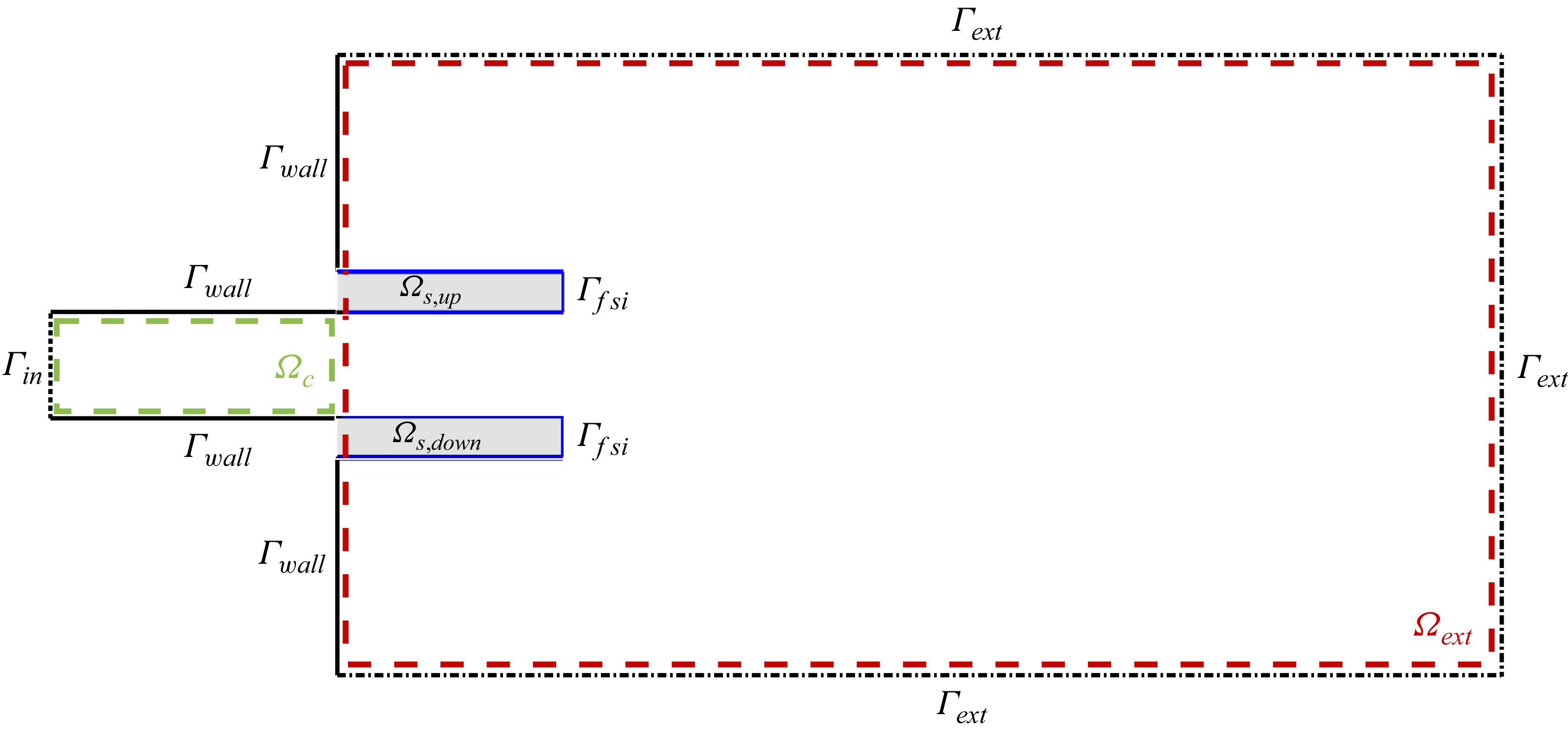
Schematic representation of the reference configuration (not to scale): reference fluid domain
 $\varOmega _{\!f,0}$
(white region) and reference solid domain
 $\varOmega _{s,0}$
(grey region). The fluid region is divided in the channel region
 $\varOmega _c$
(green dashed boundary) and the external region
 $\varOmega _\textit{ext}$
(red dashed boundary)
 $\setminus \varOmega _{s,0}$
. The solid region is divided in
 $\varOmega _\textit{s,up}$
and
 $\varOmega _\textit{s,down}$
. Boundary definition: inlet
 $\varGamma _\textit{in}$
(dotted line), no-slip walls
 $\varGamma _{w\textit{all}}$
(continuous black lines), fluid–structure interface
 $\varGamma _\textit{fsi}$
(continuous blue lines) and external stress-free boundaries
 $\varGamma _\textit{ext}$
(dashed–dotted lines).

For each time step, it is possible to transform each variable defined in the reference configuration into the corresponding one in the deformed configuration exploiting the aforementioned family of mappings. For the fluid domain, we can state that the deformed configuration is obtained from the reference, undeformed one by virtue of a displacement field that depends on time,
 \begin{equation} \mathcal{A}_t(\boldsymbol{\chi },t) = \boldsymbol {x}(\boldsymbol{\chi },t) = \boldsymbol{\chi } + \boldsymbol{\xi }(\boldsymbol{\chi },t), \quad \text{in } \quad \varOmega _{\!f,0}, \end{equation}
where
 $\boldsymbol{\xi }$
represents the displacement at time
 $t$
. This approach requires the solution of an additional equation for the displacement
 $\boldsymbol{\xi }$
in order to extend to the fluid domain the displacement in the solid. In the structure domain, the
 $\mathcal{A}_t$
map is simply defined based on the structure displacement,
 \begin{equation} \mathcal{A}_t(\boldsymbol{\chi },t) = \boldsymbol {x}(\boldsymbol{\chi },t) = \boldsymbol{\chi } + \boldsymbol{s}(\boldsymbol{\chi },t), \quad \text{in } \quad \varOmega _{s,0}. \end{equation}
The three subproblems (fluid, structure and mapping of the fluid domain) are fully coupled in a single, monolithic, three-field formulation. Each problem is formulated in weak form and all the equations are collected together. In this way, the full state of the system is
 \begin{equation} \boldsymbol{q} = (\boldsymbol{q_s},\boldsymbol{q_{\!f}},\boldsymbol{q_e})\quad \textrm {with}\quad \boldsymbol{q_s}=(\boldsymbol{s},\boldsymbol{u_s}),\;\boldsymbol{q_{\!f}} = (\boldsymbol{u},p,\boldsymbol{\lambda })\quad \textrm {and}\quad \boldsymbol{q_e} = (\boldsymbol{\xi },\boldsymbol{\lambda _e}). \end{equation}
In particular,
 $\boldsymbol{q_s}$
is the structural state defined by the solid displacement
 $\boldsymbol{s}$
and velocity
 $\boldsymbol{u_s}$
. The fluid state
 $\boldsymbol{q_{\!f}}$
collects the fluid velocity and pressure together with the Lagrange multiplier
 $\boldsymbol{\lambda }$
needed to enforce the stress continuity on the fluid–structure interface,
 $\varGamma _\textit{fsi}$
. The unknowns describing the mapping of the fluid domain are collected in
 $\boldsymbol{q_e} = (\boldsymbol{\xi },\boldsymbol{\lambda _e})$
, where
 $\boldsymbol{\xi }$
denotes the displacement and
 $\boldsymbol{\lambda _e}$
the Lagrange multiplier needed to enforce the Dirichlet boundary condition for the displacement on the fluid–structure interface,
 $\boldsymbol{s} = \boldsymbol{\xi }$
on
 $\varGamma _\textit{fsi}$
. The stress continuity is enforced in a weak sense. Indeed, the boundary term on the fluid–structure interface is substituted by the Lagrangian multiplier
 $\boldsymbol{\lambda }$
in the fluid and solid weak formulations while the boundary condition for the continuity of the velocity
 $\boldsymbol{u} = \boldsymbol{u_s}$
on
 $\varGamma _\textit{fsi}$
is the additional equation required for the additional unknown. The Dirichlet boundary conditions for the fluid velocity at the inlet
 $\varGamma _\textit{in}$
, see figure 2, and for the structural displacement at the clamped edge are imposed by additional lifting terms. We consider the incompressible Navier–Stokes equations (INSE) to describe the flow field in the fluid domain
 ${\varOmega \!}_f(t)$
:
 \begin{equation} \begin{cases} \dfrac {\partial \boldsymbol{u}}{\partial t} + (\boldsymbol{u}\boldsymbol{\cdot }\boldsymbol{\nabla })\boldsymbol{u} = -\boldsymbol{\nabla \!}p + \dfrac {1}{\textit{Re}} \boldsymbol{\nabla }\boldsymbol{\cdot }( \boldsymbol{\nabla }\boldsymbol{u}+\boldsymbol{\nabla }\boldsymbol{u}^T),\\ \boldsymbol{\nabla }\boldsymbol{\cdot }\boldsymbol{u} = 0. \end{cases} \end{equation}
In the present paper, the average, bulk fluid speed at the inlet
 $U_\infty$
is selected as reference velocity and the undeformed channel height
 $H$
is used as the reference length. The INSE have been made dimensionless by the reference velocity
 $U_{\infty }$
, the length
 $H$
and the density
 $\rho _{\!f}$
. The dimensionless Reynolds number reads
 \begin{equation} \textit{Re} = \frac {\rho _{\!f}U_{\infty }H}{\mu _{\!f}}, \end{equation}
where
 $\mu _{\!f}$
is the fluid dynamic viscosity. The system (2.6) is written in a fixed, reference, initial configuration
 $\varOmega _{\!f,0}$
, as done by Pfister, Marquet & Carini (Reference Pfister, Marquet and Carini2019) using the mapping (2.3). The structural behaviour of an isotropic material with Young’s modulus
 $E_s$
and Poisson ratio
 $\nu$
is described by the elasticity equation. The Poisson ratio gives a measure of the deformation of the structure in the directions perpendicular to the one of the applied loadings. In the same manner as we did for the INSE, the deformed configuration at each time step is described by the structural displacement field
 $\boldsymbol{s}$
, with the map (2.4). Hence, the linear elasticity is solved in the stress-free reference domain
 $\varOmega _{s,0}$
,
 \begin{equation} \begin{cases} m^*\,\dfrac {\partial \boldsymbol{u_s}}{\partial t} = \boldsymbol{\nabla }\boldsymbol{\cdot }\boldsymbol{P},\\ \dfrac {\partial \boldsymbol{s}}{\partial t} = \boldsymbol{u_s}, \end{cases} \end{equation}
where
 $m^*$
is the dimensionless mass ratio,
 \begin{equation} m^* = \frac {\rho _s}{\rho _{\!f}}, \end{equation}
with
 $\rho _s$
the solid density. The structure equations are made dimensionless and the dimensionless Young’s modulus
 $E$
is introduced,
 \begin{equation} E = \frac {E_s}{\rho _{\!f}U_{\infty }^2}. \end{equation}
In (2.8), the variables
 $\boldsymbol{s}$
and
 $\boldsymbol{u_s}$
are the structural displacement and the velocity, respectively, while
 $\boldsymbol{P}$
is the first Piola–Kirchoff stress tensor. A hyperelastic Saint Venant–Kirchoff structural model is adopted to describe the relationship between the deformations and the stresses in the material. From the Saint Venant–Kirchoff model, we can write
 $\boldsymbol{P}$
as a function of the second Piola–Kirchoff stress tensor
 $\boldsymbol{S} = \lambda tr(\boldsymbol{E})\boldsymbol{I} + 2\mu \boldsymbol{E}$
, where
 $\boldsymbol{E} = ({1}/{2})(\boldsymbol{\nabla} _{\!\boldsymbol{\chi }}\boldsymbol{s} + (\boldsymbol{\nabla} _{\!\boldsymbol{\chi }}\boldsymbol{s})^T + (\boldsymbol{\nabla} _{\!\boldsymbol{\chi }}\boldsymbol{s})^T \boldsymbol{\nabla} _{\!\boldsymbol{\chi }}\boldsymbol{s} )$
is the Lagrangian–Green strain tensor,
 $\lambda = {E\!\nu }/[{(1+\nu )(1-2\nu )}]$
and
 $\mu = {E}/[{2(1+\nu )}]$
are the Lamé coefficients of the material. In particular,
 $\boldsymbol{P} = \mathbb{J}_{\mathcal{A}_t} \boldsymbol{S}$
, where
 $\mathbb{J}_{\mathcal{A}_t} = \boldsymbol{I} + \boldsymbol{\nabla} _{\!\boldsymbol{\chi }} \boldsymbol{s}$
is the deformation gradient in the structure. The symbol
 $\boldsymbol{\nabla} _{\!\boldsymbol{\chi }}$
denotes the gradient of a vector field in the reference configuration. As previously stated, the ALE formulation allows us to rewrite the problem in a fixed, reference configuration
 $\varOmega _{0}$
by virtue of the map
 $\mathcal{A}_t$
. The domain displacement field
 $\boldsymbol{\xi }$
is obtained solving the extension problem,
 \begin{equation} \boldsymbol{\nabla }\boldsymbol{\cdot }\varSigma (\boldsymbol{\xi }) = 0 \quad \text{in} \quad \varOmega _{\!f,0}, \end{equation}
with boundary conditions
 \begin{equation} \begin{cases} \boldsymbol{\xi } = \boldsymbol{s} &\text{in } \quad \varGamma _\textit{fsi},\\ \boldsymbol{\xi } = 0, &\text{in } \quad \partial \varOmega _{\!f,0} \,- \,\varGamma _\textit{fsi}, \end{cases} \end{equation}
where
 $\varSigma (\boldsymbol{\xi })$
is an extension operator used to extend the structure displacement from the fluid–structure interface
 $\varGamma _\textit{fsi}$
into the fluid domain. In the present case, we did not solve (2.11) in the whole fluid domain, to reduce the computational cost, but the domain considered is restricted to a region delimited by a vertical line at
 $x=\bar {x}=50$
. For
 $x\gt \bar {x}$
, a null mesh displacement is considered and the usual INSE (2.6) are solved. The operator
 $\varSigma$
in (2.11) is in general arbitrary. We solved the flow-domain displacement problem using a linear elasticity extension operator,
 \begin{equation} \boldsymbol{\nabla }\boldsymbol{\cdot }\varSigma (\boldsymbol{\xi }) = \boldsymbol{\nabla }\boldsymbol{\cdot }(\lambda _{e} \,\textrm {tr}(\boldsymbol{\varepsilon _e})\boldsymbol{I} + 2\mu _e \boldsymbol{\varepsilon _e}), \end{equation}
where
 $\boldsymbol{\varepsilon _e} = \boldsymbol{\nabla }\boldsymbol{\xi } + \boldsymbol{\nabla }\boldsymbol{\xi }^T$
is the linear strain tensor and
 $\lambda _{e}= {E_e \nu _e}/[{(1+\nu _e)(1-2\nu _e)}],\mu _{e}= {E_e}/[{2(1+\nu _e)}]$
the Lamè coefficient for the displacement equation, that is computed with a fixed Poisson ratio
 $\nu _e=0.35$
and a stiffness
 $E_e(\boldsymbol{\chi })$
that depends on the distance from the fluid–structure interface. The flow-domain displacement stiffness is tuned to avoid excessive mesh distortion for the small triangular elements near the moving structure. Other extension operators can be used in (2.13) (see Shamanskiy & Simeon Reference Shamanskiy and Simeon2020), with the Laplace operator that is the simplest option. However, the present choice guarantees an increased robustness in the nonlinear simulations. In particular, the computation of a distance from the fluid–structure interface is performed solving a Laplacian problem for the variable
 $E_e(\boldsymbol{\chi })$
with Dirichlet boundary condition
 $E_e=10^6$
on the interface and
 $E_e=1$
on the line
 $x=\bar {x}$
that delimits the domain of interest where the flow-domain displacement problem is solved. On the other boundaries of the flow domain, we impose homogeneous Neumann boundary conditions.
2.1. Computational set-up
The geometrical configuration in the initial, undeformed shape is shown in figure 1. Such configuration defines the initial fluid domain
 $\varOmega _{\!f,0}$
and the stress-free structural domain
 $\varOmega _{s,0}$
that are used as reference domains where all the equations are written and discretised so that
 $\varOmega _0 = \varOmega _{s,0} \cup \varOmega _{\!f,0}$
. The flexible nozzle is made of two identical plates. Their length and thickness are
 $L_{\!p} = 5$
and
 $t_p=0.1$
, respectively. The plates are clamped in
 $x=0$
and placed with their centreline at
 $y = \pm 0.55$
. They define two distinct structural domains
 $\varOmega _\textit{s,up} = [0,\,L_{\!p}]\times [0.55 - t_p/2,\,0.55 + t_p/2 ]$
and
 $\varOmega _\textit{s,down} = [0,\,L_{\!p}]\times [-0.55 - t_p/2,\,-0.55 + t_p/2 ]$
. The reference structural domain is thus defined as
 $\varOmega _{s,0} = \varOmega _\textit{s,up}\cup \varOmega _\textit{s,down}$
. The plate mass ratio is
 $m^*=20$
and the Poisson ratio is kept fixed at
 $\nu =0.4$
. The fluid domain consists of an initial channel of height
 $H=1$
and length
 $L_0=10$
that describes the domain
 $\varOmega _c = [-L_0,\,0] \times [-H/2,\,H/2]$
, and a rectangular domain
 $\varOmega _\textit{ext} = [0,\,2500] \times [-50,\,50]$
that describes the outer region where the jet exits. To precisely define the outer fluid domain, we have to remove from
 $\varOmega _\textit{ext}$
the structure domain
 $\varOmega _{s,0}$
. A parabolic velocity profile
 $u(y) = ({3}/{2})(1-4y^2)$
is used as inlet condition at
 $x = -L_0$
(
 $\varGamma _\textit{in}$
in figure 2). Homogeneous Dirichlet boundary conditions are enforced on the undeformed top and bottom wall
 $\varGamma _{w\textit{all}}$
in the channel, at
 $|y|=H/2$
. In the outer region, a no-slip boundary condition is used at
 $x = 0$
and
 $|y| \gt 0.6$
. In the top and bottom sides of the outer domain
 $\varOmega _0$
and at the right-hand boundary
 $x=2500$
, a stress-free condition is enforced. The finite element, open-source library GetFEM (Renard & Poulios Reference Renard and Poulios2020) has been used to implement the ALE scheme and run all the simulations. The fluid mesh is generated with the anisotropic mesh generator BAMG available in the FreeFem++ software (Hecht Reference Hecht2012). Moreover, the mesh is symmetrically generated with respect to the axis
 $y=0$
to preserve the symmetry of the problem to machine precision.
2.2. Linear stability analysis
The stability of the fixed points of the nonlinear, monolithic system
 $M(\boldsymbol{q})\,\dot {\boldsymbol{q}} = \boldsymbol{f}(\boldsymbol{q})$
for
 $\boldsymbol{q}$
defined in (2.5) is investigated by means of the LSA and normal-mode decomposition (Fabre et al. Reference Fabre, Citro, Ferreira Sabino, Bonnefis, Sierra, Giannetti and Pigou2019). We denote the size of the state vector
 $\boldsymbol{q}$
with
 $N$
. The fixed points, i.e. steady states of the monolithic FSI system, are computed from the steady, nonlinear system obtained dropping the time derivatives and discretising in space the INSE (2.6), the elasticity (2.8) and the flow-domain displacement problem (2.11) in the reference configuration. We obtain a nonlinear system
 $\boldsymbol{f}(\boldsymbol{q})=0$
that we solve by a Newton–Raphson iteration, attaining the steady state solution
 $\boldsymbol{q_0}$
. Once the base flow has been computed, we investigate the fate of a small disturbance of the steady state
 $\boldsymbol{q_0}$
. The equations are linearised around that solution and an eigenvalue problem (EVP) is retrieved by a modal decomposition of the solution
 $\boldsymbol{q}(\boldsymbol{\chi },t) \approx \boldsymbol{q_0}(\boldsymbol{\chi }) + \epsilon \boldsymbol{q'(\boldsymbol{\chi },t)} = \boldsymbol{q_0}(\boldsymbol{\chi }) + \epsilon (\boldsymbol{\hat {q}}(\boldsymbol{\chi })e^{\lambda t} +\text{ c.c.})$
, where the higher-order terms in
 $\epsilon$
are neglected and
 $\text{ c.c.}$
indicates complex conjugate terms. In our analysis, we considered only two-dimensional (2-D) perturbations
 $\boldsymbol{\hat {q}(\boldsymbol{\chi })}$
. In this formulation,
 $\lambda \in \mathbb{C}$
is the eigenvalue and
 $\boldsymbol{\hat {q}} \in \mathbb{C}^N$
the associated eigenvector of the following EVP:
 \begin{equation} \lambda M(\boldsymbol{q_0})\boldsymbol{\hat {q}} = \boldsymbol{f}'(\boldsymbol{q_0}) \boldsymbol{\hat {q}}, \end{equation}
where
 $\boldsymbol{f}'(\boldsymbol{q_0})$
is the tangent matrix of the nonlinear system and
 $M(\boldsymbol{q_0})$
is the mass matrix, both evaluated at the steady state under consideration. The linearisation of the FSI system is performed and the EVP is solved in the same reference, undeformed configuration. For the disturbances, homogeneous Dirichlet boundary conditions are enforced at the inlet and on the rigid walls. A no-stress condition is enforced on the top and bottom sides of the outer region and on the outlet. On the FSI interface, the continuity of the stresses and of the velocity is assumed, while for the flow-domain subproblem, the continuity of the displacement from the structure to the fluid domain is enforced. Moreover, the adjoint EVP is solved to complete the global-mode stability analysis,
 \begin{equation} \lambda ^* M(\boldsymbol{q_0})^T\boldsymbol{\hat {q}^\dagger } = \boldsymbol{f}'(\boldsymbol{q_0})^T \boldsymbol{\hat {q}}^\dagger , \end{equation}
where the symbol
 $^*$
stands for complex conjugate and
 $^T$
indicates the transpose operator. Indeed, the adjoint problem gives us information about the region of the space where there is the highest receptivity of a global mode to external forcing (Luchini & Bottaro Reference Luchini and Bottaro2014). Then, the identification of the wavemaker region is obtained combining the information coming from the direct mode with the receptivity map obtained by the adjoint eigensolutions by computing the structural-sensitivity field
 \begin{equation} S(\boldsymbol{\chi })= \begin{cases} \| \boldsymbol{\hat {u}}^\dagger (\boldsymbol{\chi }) \| \ \| \boldsymbol{\hat {u}}(\boldsymbol{\chi }) \| \quad & \text{in} \quad \varOmega _{\!f,0}, \\ \| \boldsymbol{\hat {u}_s}^\dagger (\boldsymbol{\chi }) \| \ \| \boldsymbol{\hat {u}_s}(\boldsymbol{\chi }) \| \quad & \text{in} \quad \varOmega _{s,0}, \end{cases} \end{equation}
where
 $\| . \|$
represents the usual
 $\mathbb{R}^2$
vector norm,
 $\boldsymbol{\hat {u}}(\boldsymbol{\chi })$
and
 $\boldsymbol{\hat {u}}^\dagger (\boldsymbol{\chi })$
represent the fluid velocity contribution to the direct and adjoint eigenvectors while
 $\boldsymbol{\hat {u}_s}(\boldsymbol{\chi })$
and
 $\boldsymbol{\hat {u}_s}^\dagger (\boldsymbol{\chi })$
represent the solid velocity contribution. In this manner, the structural sensitivity is extended also in the structural domain and the continuity of velocity ensures the smoothness of this field. Note that the normalisation coefficient used in the definition of the structural sensitivity by Giannetti & Luchini (Reference Giannetti and Luchini2007) is not reported in the definition of
 $S(\boldsymbol{\chi })$
in (2.16) because we normalised the eigenvectors to satisfy
 $(\boldsymbol{\hat {q}}^\dagger ,\boldsymbol{\hat {q}})=1$
. Large values of
 $S$
identify the region of the flow where disturbance amplification and receptivity combine at their best to trigger the instability. Such an approach, first proposed by Giannetti & Luchini (Reference Giannetti and Luchini2007) for the cylinder-wake instability, isolates the regions in the domain where a modification of the structure of the problem produces the largest drift of the eigenvalue. Hence, such an approach can be used to identify where the core of the instability mechanism is located (Fabre et al. Reference Fabre, Citro, Ferreira Sabino, Bonnefis, Sierra, Giannetti and Pigou2019). This approach has been extended for FSI by Pfister (Reference Pfister2019) to evaluate the receptivity region of a structural modification of the EVP also in the structural domain. We note that the elasticity operator by itself is self-adjoint, hence the direct and adjoint modes coincide and the structural sensitivity coincided with the mode. In the case of FSI, this is no longer true because of the coupling with the incompressible Navier–Stokes operator. However, in the present case the direct and the adjoint modes are not very different in the structure and the maximum overlap is located in the region where the structure moves the most, in the free end of the plates.
3. Results
3.1. Base flow
We start to present the base flow. The base flow is symmetrical with respect to the channel axis, with the upper plate that bends upwards and the lower one that bends downwards. No symmetry-breaking mechanisms leading to a steady asymmetric solution, and associated with a critical real eigenvalue, have been observed in the space of parameters considered. The flexibility tends to increase the channel cross-section with respect to the rigid configuration. Indeed, the channel is deformed by the high-pressure inside it, produced by the head loss. The head loss is due to viscous effects which lead to a pressure gradient inside the channel. Such a high-pressure distribution is not balanced by the external pressure and therefore tends to deflect the plates, opening the channel, until an equilibrium with the restoring elastic forces is reached. In figure 3, we show the vertical displacement
 $s_y$
of the upper-plate free end measured on the neutral axis of the plate. We observe that the deformation increases when the Reynolds number is decreased, due to the increasing viscous effects, and when the Young’s modulus is decreased due to a more flexible structure. We note that, reducing the plate stiffness, a threshold depending on
 $\textit{Re}$
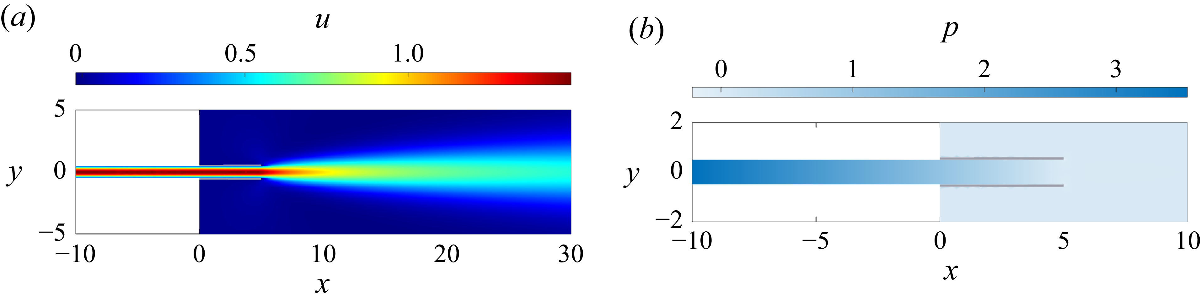
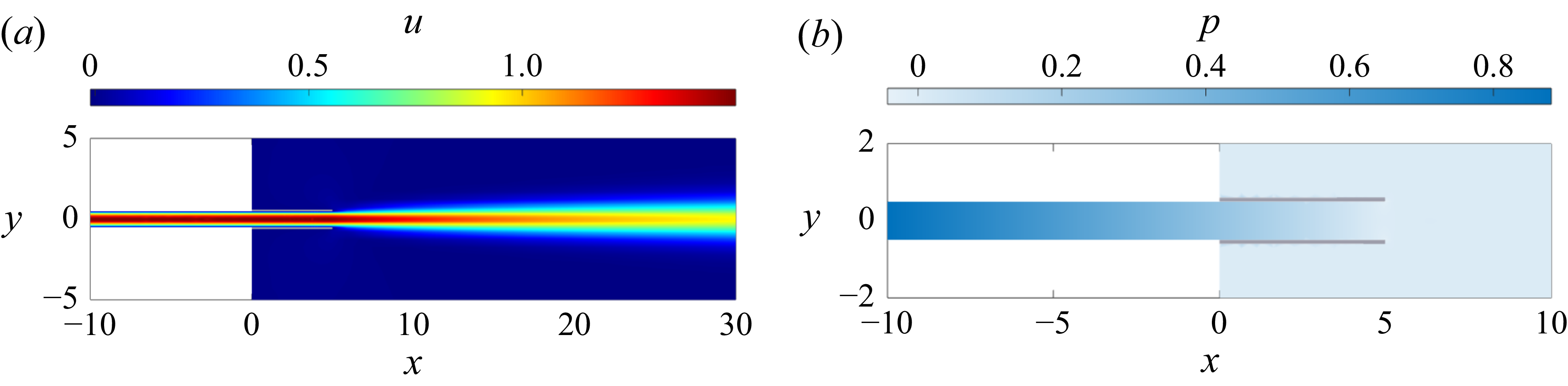
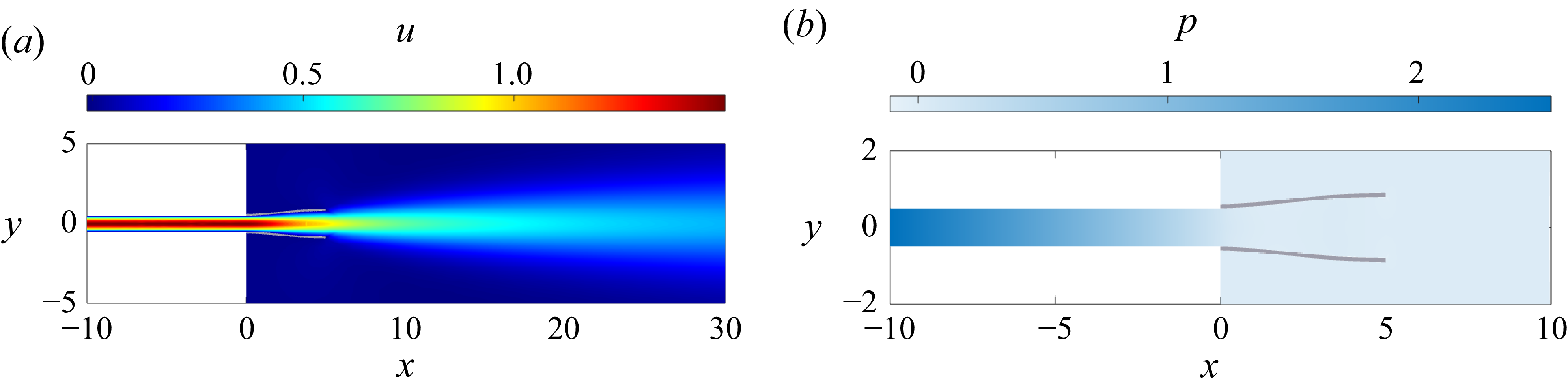
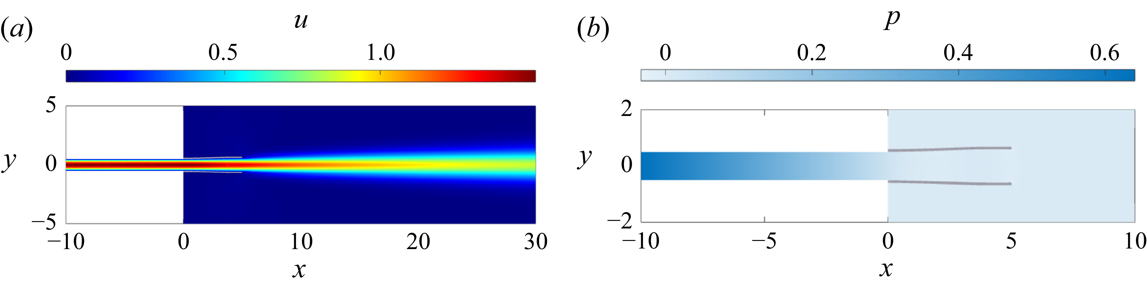
is reached, above which the free end deformation of the channel is almost constant with the stiffness. Below this threshold, the channel opens enough to almost annihilate the pressure gradient in the deformable part of the channel. In figure 3, we mark with a red star the four points, labelled A, B, C and D, we chose to analyse the base flow in detail. Such points have been chosen to compare a very rigid configuration for two different Reynolds numbers 50, point A, and 200, point B, with a very flexible configuration at the same Reynolds numbers, points C and D, respectively. The different base flows for a rigid configuration
 $E=10^8$
are shown in figure 4 (A) for
 $\textit{Re}=50$
and in figure 5 (B) for
 $\textit{Re}=200$
. A very flexible configuration with
 $E=10^3$
for the same couple of Reynolds numbers is reported in figures 6 (C) and 7 (D). The figures show the horizontal component of the fluid velocity and the pressure distribution in the deformed configuration. In figure 8, we reported the same quantities along the nozzle centreline in order to achieve a more quantitative analysis for the four points A, B, C and D under discussion. In the rigid case, the nozzle is largely undeformed and a planar laminar jet evolves out of the nozzle. The effect of the Reynolds number on the diffusion of the jet past the exit is evident, the lower the Reynolds number the faster the diffusion of the jet. This is further clarified by the plot over the nozzle centreline in figure 8 comparing the horizontal velocity that decreases faster for the case A with respect to the case B. The pressure distribution inside the channel is linear, according to the solution of the laminar plane channel flow, and the pressure gradient depends on the Reynolds number. This is clearly visible comparing the case A and B in figure 8. Outside the nozzle, the pressure is almost constant. In the flexible configuration, the base flow is quite different. The nozzle structural deformation significantly modifies the evolution of the flow, with a strong effect in the region inside the nozzle. At the same time, in the flexible configuration, varying the Reynolds number produces a large base flow modification. Indeed, decreasing the Reynolds number increases the nozzle deformation. The base flow for
 $E=10^3$
and
 $\textit{Re}=50$
(C) is shown in figure 6. In this case, the nozzle is strongly deformed by the flow, with an outflow cross-section that is approximately
 $1.7$
times larger with respect to the undeformed one. The jet flow starts spreading farther upstream with respect to the rigid case. This physical phenomenon is clarified comparing the case C with its rigid counterpart at the same Reynolds number (case A). In figure 8, we observe that the fluid velocity starts to decrease far upstream with respect to the rigid configuration due to the fact that the nozzle is so flexible that the ends of the plates separate significantly. The deformation of the nozzle that reduces the head losses is also highlighted by the pressure distribution inside the nozzle. Indeed, in the most flexible case, the linear pressure distribution of the channel flow is recovered only in the initial undeformed duct, and the flow inside the flexible nozzle has an almost constant pressure distribution, visible in figure 8. For a larger Reynolds number, see for instance
 $\textit{Re}=200$
(D) in figure 7, the base flow shares similar properties with the low
 $\textit{Re}$
case, with a deformed nozzle with an almost constant pressure distribution inside it, as visible in figure 8. However, in this case, the deformation of the nozzle is by far smaller, with an outflow cross-section which is less than
 $20\,\%$
larger than the undeformed one. This is due to the fact that, while also in this case the jet starts to spread upstream with respect to the rigid case, its diffusion is less than for a lower Reynolds number. For intermediate stiffness and Reynolds number, intermediate base flow properties are observed.
Base flow: vertical displacement (
 $s_y$
) of the upper-plate free end.

Base flow (A): a rigid configuration for
 $E=10^8$
and
 $\textit{Re}=50$
. Horizontal velocity component (a) and pressure (b).

Base flow (B): a rigid configuration for
 $E=10^8$
and
 $\textit{Re}=200$
. Horizontal velocity component (a) and pressure (b).

Base flow (C): a flexible configuration
 $E=10^3$
and
 $\textit{Re}=50$
. Horizontal velocity component (a) and pressure (b).

Base flow (D): a flexible configuration
 $E=10^3$
and
 $\textit{Re}=200$
. Horizontal velocity component (a) and pressure (b).

Spatial evolution of the horizontal velocity (a) and pressure (b) fields along the centreline of the nozzle for the points A, B, C and D.

3.1.1. Simplified quasi-1-D model
We compared the numerical results obtained using the ALE with a quasi-1-D model designed specifically for the present flow configuration. To model this FSI problem, we drew inspiration from the work of Luchini & Charru (Reference Luchini and Charru2010), which addresses quasi-
1-D equations for laminar flow. The authors formulated section-averaged equations of motion and showed that, by an appropriate multiple-scale expansion, a first-order accurate approximation can be obtained for the pressure gradient inside a symmetric, slowly varying duct, without an explicit knowledge of the velocity field. This result is obtained showing that the continuity equation and the energy equation in the section-averaged formulation are indeed first-order accurate equations while the momentum equation is not, providing that the boundary is either a solid or a stress-free surface. In the case of a moving solid surface, Luchini & Charru (Reference Luchini and Charru2010) demonstrated that the model remains valid provided the longitudinal wall velocity is of order
 $O(\epsilon ^2)$
. We exploit these results, considering the Euler–Bernoulli (EB) elasticity equation together with the section averaged INSE for a slow varying duct. In this formulation, we use only pressure forces to load the structure. In this way, the multiple-scale expansion allows us to compute a first-order accurate solution taking into account the pressure correction due to the nozzle opening. Let us consider a 2-D symmetric duct with symmetry axis
 $y=0$
and a wall at
 $y=h(x,\,t)$
. Let us denote the longitudinal flow velocity with
 $u(x,y,t)$
and the pressure field with
 $P(x,y,t)$
. The integral mass, momentum and kinetic-energy balance equations read
 \begin{equation} \frac {\partial h}{\partial t} + \frac {\partial }{\partial x} \int _0^h u \,{\rm d}y\,=\,0, \end{equation}
 \begin{equation} \frac {\partial }{\partial t} \int _0^h u \,{\rm d}y\, + \,\frac {\partial }{\partial x} \int _0^h u^2 \,{\rm d}y\, + \int _0^h P_x \,{\rm d}y\,=\,-\tau \, = \,\frac {1}{\textit{Re}}u_y(h), \end{equation}
 \begin{equation} \frac {\partial }{\partial t} \int _0^h \frac {u^2}{2} \,{\rm d}y\, + \,\frac {\partial }{\partial x} \int _0^h \frac {u^3}{2} \,{\rm d}y\, + \int _0^h u \,P_x \,{\rm d}y\,=\,-f\, = \,-\frac {1}{\textit{Re}}\int _0^h u^2_y\, {\rm d}y, \end{equation}
where
 $\tau$
is the wall shear stress and
 $f$
is the dissipation function. Luchini & Charru (Reference Luchini and Charru2010) considered a multiple-scale expansion in which the time
 $t$
and the axial coordinate
 $x$
are rescaled by an arbitrarily small parameter
 $\epsilon$
and replaced by
 $T/\epsilon$
and
 $X/\epsilon$
, with
 $T$
and
 $X$
the
 $O(1)$
rescaled coordinates. Then, a power series expansion in
 $\epsilon$
is introduced for the different terms. For instance, the longitudinal velocity is approximated at first order as
 $u(x,y,t) \,\approx \, u^{(0)}(x,y,t) \,+\, \epsilon u^{(1)}(x,y,t)$
.
A Poiseuille parabolic profile is assumed for the zero-order longitudinal velocity
 $u^{(0)}(x,y,t) = ({3}/{2})U(x,t)(1-y^2/h^2)$
, where
 $U(x,t)$
denotes the average velocity in the cross-section. Introducing the rescaled coordinates
 $T$
and
 $X$
and the power series expansion in the (3.1), (3.2) and (3.3), one can extract the multiple-scale expansion for such system of equations at each desired order. Luchini & Charru (Reference Luchini and Charru2010) showed that the section-averaged continuity and the kinetic-energy balance equations,
 \begin{equation} \frac {\partial h}{\partial t} + \frac {\partial (hU)}{\partial x} = 0, \end{equation}
 \begin{equation} \dfrac {6}{5}\frac {\partial }{\partial t}\dfrac {hU^2}{2} +\frac {54}{35} \frac {\partial }{\partial x}\frac {hU^3}{2} + hUP_x = -\frac {3U^2}{\textit{Re} h}, \end{equation}
are indeed first-order accurate equations for the pressure
 $P\approx P^{(0)} + \epsilon P^{(1)}$
, providing
 $U(x,t)$
is the true mean velocity in the cross-section (the flow rate of
 $u^{(1)}$
is null) and the boundaries of the channel are a solid or stress-free surface. The EB beam model for the plate, forced by the pressure distribution along the channel, reads
 \begin{equation} m \frac {\partial ^2 h}{\partial t^2} + \textit{EI} \frac {\partial ^4 h}{\partial x^4} = P. \end{equation}
In (3.6),
 $m$
is the mass of the beam per unit length and
 $EI$
is its bending stiffness. In this case, we considered the pressure inside the nozzle as the sole external load on the flexible structure. The external fluid pressure
 $P$
is assumed to be null. Hence, for the quasi-1-D model, we solved the system of (3.4), (3.5) and (3.6) with a finite element method on a 1-D grid
 $\varOmega _{1D}\in [0,\,L_{\!p}]$
, discretised by
 $5000$
uniformly distributed elements. We used
 $\mathbb{P}_2$
elements for the velocity and displacement fields, and for the second derivative of the latter, while
 $\mathbb{P}_1$
elements for the pressure, for a total number of
 $35\,000$
degrees of freedom, approximately. The great advantage of this formulation is that it does not require us to compute the first-order velocity approximation to compute the first-order pressure distribution because the first-order correction of the dissipation function,
 \begin{equation} f^{(1)} = \frac {2}{\textit{Re}} \int _0^h u_y^{(0)} u_y^{(1)}{\rm d}y\, , \end{equation}
is null, while the wall shear stress correction
 \begin{equation} \tau ^{(1)} = -\frac {1}{\textit{Re}} u_y^{(1)}(h) \end{equation}
is not (Luchini & Charru Reference Luchini and Charru2010). However, once the (3.4) and (3.5) are solved, the momentum balance equation can still be used to compute the wall shear stresses up to the first order:
 \begin{equation} \tau \approx \tau ^{(0)} + \epsilon \tau ^{(1)} = -\Big ( \frac {\partial }{\partial t}(hU) +\frac {6}{5} \frac {\partial }{\partial x}(hU^2) + h\,P_x \Big ). \end{equation}
Lastly, from the multiple-scale expansion of the momentum equation in the
 $y$
direction, not reported here for conciseness, one deduces that the pressure field does not vary in the cross-section for the zero- and first-order terms, i.e.
 $\partial _y P^{(0)} = \partial _y P^{(1)} = 0$
.
We have to supplement the model with proper boundary conditions. For the fluid, a bulk velocity
 $U=1$
at the inlet
 $\varGamma _\textit{in}$
at
 $x=0$
is considered, while a pressure condition
 $P=0$
is enforced at the outlet at
 $x=L_{\!p}$
. For the structure, a clamped end with the undeformed channel height
 $h(0,t)=H/2$
is enforced at
 $x=0$
. Due to this condition, the rotation of the beam is avoided in this point and
 $h_x(0,t)=0$
. In the free end in
 $x=L_{\!p}$
, null shear and moment are enforced,
 $h_{\textit{xx}}(L_{\!p},t)=h_{\textit{xxx}}(L_{\!p},t)=0$
. We used a Newton iteration to solve the ensuing nonlinear system. In figure 9, the results of the quasi-1-D model (red points), are compared with the ALE results (blue points). From the comparison, we note the overall agreement of the ALE results with the quasi-1-D model by Luchini & Charru (Reference Luchini and Charru2010), especially for the highest Reynolds numbers and stiffness values, allowing us to reconstruct the deformed configuration with reasonable accuracy as a function of the Reynolds number and structural flexibility. In particular, the model predicts well the change in the curvature of the curve obtained from
 $s_y(E,\textit{Re})$
keeping fixed the Reynolds number. Moreover, for the largest Reynolds number considered here, the theoretical results fit very accurately the beam displacement of the ALE ones. This is not completely the case going towards smaller values of the Reynolds number. Indeed, the quasi-1-D model predicts free end displacements larger than those obtained with the ALE, with a discrepancy between the two results that increases as the Reynolds number decreases. One possible reason of the discrepancy could be the pressure boundary condition enforced at the outlet. Indeed, in the ALE results, the pressure is not uniform in the exit cross-section, its distribution being strongly affected by the outflow near the corners of the nozzle where we observed a local region of low pressure that affects the pressure outlet condition and consequently the loads on the structure. This issue warrants further investigation which is deferred to future work.
Base flow: upper-plate free end vertical displacement (
 $s_y$
) as a function of the plate stiffness and of the Reynolds number. Full ALE formulation, blue dots; quasi-1-D model, red dots.

3.2. Linear stability analysis
The LSA is performed tracking the leading four Hopf bifurcations as a function of the control parameters. We draw their neutral curves by continuation in the parameter space, as shown in figure 10(a). As illustrated in figure 11, the first four modes for this configuration include a couple of sinuous modes that become unstable owing to the flutter of the second and fourth bending modes of the cantilevered beams, and a couple of varicose modes associated with the third and fourth bending modes of the beams. By flutter mode we refer to single mode flutter instability shown for cantilevered pipes by Paidoussis (Reference Paidoussis2004). The destabilisation by a single mode flutter is further clarified by a root locus analysis, reported in Appendix C. Interestingly, in the parameter range investigated here, the first bending mode did not produce any instability. The appearance of sinuous and varicose modes is a well-known feature of plane jets, as observed by Sato (Reference Sato1960). However, in the absence of elastic boundaries, all modes remain globally stable, and the flow experiences only convective instabilities (Huerre & Monkewitz Reference Huerre and Monkewitz1990). Here, we observe that the planar jet in the FSI context can become absolutely unstable due to the interaction with the flexible nozzle. In the framework of a global stability analysis, the emergence of an absolute instability is signalled by a real eigenvalue or a pair of complex conjugate eigenvalues crossing the imaginary axis (Huerre & Monkewitz Reference Huerre and Monkewitz1990). The critical stiffness
 $E_c$
of each mode at the instability threshold depends on the Reynolds number. For
 $\textit{Re}=200$
, the primary instability is due to the sinuous mode II, named in this way due its link with the second bending mode. The varicose mode III is the next to become unstable as the plate stiffness is reduced. Reducing the Reynolds number, the dominant mode becomes the varicose mode for
 $\textit{Re} \lt 41.5$
. When the plate is even more flexible, the same behaviour is found for the fourth and fifth structural bending modes, that lead to the tertiary and quaternary instability associated with the sinuous mode IV and the varicose mode V, respectively. Also in this case, the varicose mode becomes more unstable than the sinuous one at low Reynolds numbers (
 $\textit{Re} \lt 95.5$
). The lock-in of these modes with the corresponding structural bending modes is verified by comparing the frequency of the unstable modes with the natural frequencies of the structure, as reported in figure 10(b). We notice that, in computing the natural frequencies of the structure, we have accounted for the effect of the added mass of the surrounding fluid. Following De Langre (Reference De Langre2001), we can compute this effect using the potential flow theory. For an infinite oscillating plate, results are obtained in closed form by imposing the plate movement at a prescribed wavelength and evaluating the kinetic energy of the fluid, see for instance Rayleigh (Reference Rayleigh1878) and Yadykin, Tenetov & Levin (Reference Yadykin, Tenetov and Levin2003). As visible in figure 10(b), good agreement is found between the frequency computed numerically by the LSA and the analytical prediction of the EB bending modes comprehensive of the added mass effect. Due to the large displacements observed in the steady states, a finer comparison with the natural bending modes could be performed taking into account also the effect of the prestress on the natural bending modes of the plates. A deeper investigation of the added mass and prestress effect has been reported in Appendix B. However, a correction that takes into account the effect of the steady deformation is not trivial to obtain and such correction depends on the set of parameters we are looking at, making it computationally expensive to compute.
Neutral curves in the
 $\textit{Re}-E$
plane (unstable region denoted by the grey colour) (a). Frequency on the neutral curves, compared with the first five natural bending modes of the EB beam corrected by added mass effects (b) for the varicose (dashed line) and sinuous (dotted line) case. For each unstable mode we use a different colour. First sinuous, mode II (green); first varicose, mode III (blue); second sinuous, mode IV (red); second varicose, mode V (yellow).

Structural deformation for the four unstable modes. In each figure, six oscillation phases are shown, moving from the darker colour to the lighter one. Sinuous mode II for
 $\textit{Re}=150$
and
 $E=10^4$
(a), sinuous mode IV for
 $\textit{Re}=150$
and
 $E=6\times 10^2$
(b), varicose mode III for
 $\textit{Re}=200$
and
 $E=6.25\times 10^3$
(c) and varicose mode V for
 $\textit{Re}=100$
and
 $E=2\times 10^2$
(d).

In figure 11, we report the structural displacements for each global unstable mode for six phases of oscillation. As can be seen in the figure, the coupling with the fluid modifies the natural bending modes and leads to travelling waves. Indeed, for all modes, most of the nodal points along the structure where the displacement is null are suppressed by the interaction with the fluid and a travelling wave develops along the beam.
Direct (a,b) and adjoint (c,d) mode II at
 $E=10^4$
and
 $\textit{Re}=150$
. Contour of the real component of the horizontal velocity (a,c) and vertical velocity (b,d). The colour bar indicates the values of each component scaled by its maximum absolute value in the domain.

3.2.1. Sinuous modes
For this set-up, in terms of plate geometry and mass ratio
 $m^*$
, the even structural modes can lead to sinuous dynamic instabilities for sufficiently flexible plates. The sinuous modes correspond to an antisymmetrical, in-phase deformation of the plates. The first to become unstable is the one associated with the second bending mode. For this reason, we denominate it as mode II. Its deformation is reported in figure 11(a) and one can observe the two-node deformation typical of the second bending mode modified by the FSI. Indeed, while the clamped node must be a node, the second node has disappeared, so that no nodes except the clamp are left. This remark highlights that the structural bending mode has been modified to a travelling-wave mode due to FSI. The direct and adjoint modes on the neutral curve for
 $ \textit{Re} = 150$
are reported in figure 12. The peak of the direct mode is far from the flexible nozzle but shifts closer as the Reynolds number decreases. In contrast, the adjoint mode develops primarily inside the channel. The structural sensitivity, as defined by Giannetti & Luchini (Reference Giannetti and Luchini2007) is reported in figure 13. In the present case, the peak of the structural sensitivity is concentrated in two regions: in two small areas close to the flexible walls at the nozzle exit; in a large area far from the nozzle in the outflow jet region. As we will discuss in more detail later on, this is a peculiar property of the sinuous modes and it does not characterise the varicose modes. Reducing the Reynolds number, the peak in the outer jet region decreases, while the nozzle peaks remain dominant. Inside the structure, the structural sensitivity has no significant peaks and the largest contributions remain concentrated in regions in the fluid domain. This is a general trend that we observe for every global mode we found on this configuration.
Mode IV, named for its frequency content near the fourth structural mode, exhibits similar behaviour. As observed for mode II, the associated structural mode has four nodal points, as expected for the fourth bending mode. However, the interaction with the fluid modifies the dynamics of this mode so that all nodal points, but for the clamp, are eliminated. In particular, as visible in figure 11(b), the nodal point close to the free end is most affected by the interaction with the structure and presents quite large displacements. The neutral curve of mode IV resembles that of mode II, shifted to lower
 $E$
and larger
 $\textit{Re}$
. Its frequency follows the fourth structural mode corrected with added mass effects (figure 10). The structural deformation of mode IV is shown in figure 11(b), testifying the in-phase movement of the plates and the prevalent excitation of the fourth bending mode. The direct and the adjoint modes are reported in figure 14. The direct mode develops downstream of the flexible nozzle, with an antisymmetric velocity field. The adjoint mode is close to the flexible surface, both inside the channel and outside. Also in this case, the structural sensitivity (see figure 15) has a peak in the jet far from the nozzle. With respect to the previous case, however, the largest peaks of the sensitivity are located in four well defined areas symmetrically placed inside the flexible nozzle, close to the plates. These regions correspond to the regions of maximum displacement of the structure. Among them, the area closest to the clamp has the lowest peak. The shape of the structural-sensitivity field highlights the importance of the solid displacement in the instability mechanism. Indeed, the oscillation of the structure in that region is able to produce a large drift in the eigenvalue.
Mode II at
 $E=10^4$
and
 $\textit{Re}=150$
: structural sensitivity. Zoom on the nozzle region (a) and outer region (b). The colour bar denotes the structural sensitivity values scaled by its maximum value in the domain
 $S_{max}$
.

Direct (a,b) and adjoint (c,d) mode IV at
 $\textit{Re}=150$
and
 $E=6\times 10^2$
. Contour of the real component of the horizontal velocity (a,c) and vertical velocity (b,d). The colour bar indicates the values of each component scaled by its maximum absolute value in the domain.

Mode IV at
 $\textit{Re}=150$
and
 $E=6\times 10^2$
: contour of the structural sensitivity. Zoom on the nozzle region (a) and outer region (b). The colour bar denotes the structural sensitivity values scaled by its maximum value in the domain
 $S_{max}$
.

Direct (a,b) and adjoint (c,d) mode III at
 $\textit{Re}=200$
and
 $E=6.25\times 10^3$
. Contour of the real component of the horizontal velocity (a,c) and vertical velocity (b,d). The colour bar indicates the values of each component scaled by its maximum absolute value in the domain.

Direct (a,b) and adjoint (c,d) mode V at
 $\textit{Re}=100$
and
 $E=2\times 10^2$
. Contour of the real component of the horizontal velocity (a,c) and vertical velocity (b,d). The colour bar indicates the values of each component scaled by its maximum absolute value in the domain.

3.2.2. Varicose modes
The odd structural modes behave differently with respect to the even ones. Interestingly, in the region of the parameter space investigated here, the first bending mode does not become absolutely unstable. In contrast, the third and fifth bending modes couple with the flow to produce two globally unstable modes, that we denote as modes III and V, respectively. These modes share similar characteristics, with the deformation of the two beams being in opposite phase, as can be seen in figure 11. The deformation shown in the figures confirms the main excitation of the third and fifth bending modes, respectively. This is also confirmed by the analysis of the frequency content on the neutral curves, reported in figure 10, that shows the lock-in with the third and fifth structural modes. It is useful to analyse how the interaction between the fluid and the structure modifies the vibration of the latter in the unstable mode. As discussed before, this interaction leads the structure to exhibit travelling waves. This behaviour can be recognised in figure 11 from the fact that most nodal points are cancelled, with the obvious exception of the clamp. For mode III in figure 11(c), one nodal point of the two that characterise the isolated structure is still present at
 $x\approx 2$
. The second, which is closer to the free end, now exhibits quite large displacements and therefore it is no longer a node. This is a feature we observed also for the sinuous modes. For mode V in figure 11(d), the results are similar. In this case, the fifth structural bending mode has five nodal points. Also in this case, due to the interaction with the fluid, the nodal, i.e. zero displacement, points are cancelled, except at the point
 $x\approx 3.6$
and at the clamp. In this case, all the other nodal points, both the one close to the free end and those closer to the clamp, at
 $x\approx 1.25$
and
 $x\approx 2.5$
, exhibit large displacements. Moreover, as we can see in figure 10, the neutral curve of the second varicose mode is quite similar to the first one, but shifted to a smaller plate stiffness
 $E$
. Varicose modes exhibit notable differences with respect to their sinuous counterpart. First, and most important, they develop symmetrically in the flow field, as can be seen in figure 16 for mode III and in figure 17 for mode V. Second, a significant amplitude of the direct mode is observed in the area close to the walls of the flexible nozzle and in the nozzle, at all Reynolds numbers. The adjoint mode still develops close to the flexible nozzle, as observed in figures 16 and 17 for the modes III and V, respectively. The adjoint mode presents peaks for the vertical velocity component that correspond to the regions of maximum plate deflection.
In order to explain the different wavelengths exhibited by the direct modes within and outside the nozzle, we considered mode V as an example and computed the streamwise wavelength
 $\lambda _x$
as a function of the longitudinal position along the horizontal line at
 $y=0.4$
where its maxima are located inside the channel. The results are reported in figure 18, where the wavelength of the instability is plotted as a function of the longitudinal position. Crosses represent the wavelength computed as the distance between two successive maxima or two successive passages from negative to positive values. The points are quite scattered, since the unstable mode is not purely sinusoidal, but the trend compares very well with the longitudinal component of the velocity of the base flow. This observation suggests that the unstable mode behaves as a travelling wave that moves with a speed related to the base flow longitudinal velocity component in the free jet. In contrast, within the channel, the mode wavelength is dictated by the structural mode.
The structural sensitivity is reported in figure 19 for mode III and in figure 20 for mode V. Both figures show that the regions of significant structural sensitivity are limited to some areas symmetrically placed inside the nozzle, close to the walls, while the value of the structural sensitivity is insignificant far from the flexible nozzle. In particular, for mode III, the structural sensitivity has two couples of symmetric peaks that correspond to the position where the plates move the most. The structural sensitivity for mode V has also two main peaks, in striking contrast with what is observed for mode IV. Their footprint is very similar to those of mode III, but they are more distant. These peaks correspond to two areas: one located at one third of the plate length and another located at the free end. The peak at the free end is common to all modes as it corresponds to the global maximum of the plate displacement. The other peak coincides with one of the local maxima of the plate displacement. In this case, the local maxima have comparable amplitudes and therefore the mechanism responsible for the location of this peak is not evident a priori.
Mode V for
 $\textit{Re}=100$
and
 $E=2\times 10^2$
. Wavelength
 $\lambda _x$
for different longitudinal positions compared with the estimated wavelength using as phase velocity a fraction of the base flow horizontal velocity at the position
 $y=0.4$
and frequency
 $f=\lambda _i/(2\pi )$
.

Mode III at
 $E=6.25\times 10^3$
and
 $\textit{Re}=200$
: contour of the structural sensitivity. The colour bar denotes the structural sensitivity values scaled by its maximum value in the domain
 $S_{max}$
.

Mode V at
 $E=2\times 10^2$
and
 $\textit{Re}=100$
: contour of the structural sensitivity. The colour bar denotes the structural sensitivity values scaled by its maximum value in the domain
 $S_{max}$
.

3.2.3. Stability analysis by the quasi-1-D model
We exploit the quasi-1-D model also to investigate the linear stability of the coupled system, comparing the neutral curves computed with the reduced model with those obtained by the full ALE formulation. Considering that the quasi-1-D model assumes a symmetry condition on the symmetry axis, we investigate only the varicose global modes. The stability analysis of the quasi-1-D model is performed linearising the model around a steady state and investigating its stability properties by a global mode decomposition that leads to the solution of an EVP. Homogeneous Dirichlet boundary conditions are assumed for the velocity at the inlet and for the pressure at the outlet. For the structural disturbances, a null displacement and rotation are assumed in the clamped point together with null shear and moment at the nozzle free end. The implicitly restarted Arnoldi iteration implemented in the ARPACK software library has been used to solve the eigensystem. The results of the LSA on the quasi-1-D model are shown in figure 21. It is interesting to note that the simplified model predicts that two varicose global modes become unstable first, due to the travelling-wave flutter of the third and fifth structural mode, respectively. This result agrees with the results of the LSA performed on the full monolithic FSI system. Moreover, the first bending mode is globally stable as in the ALE formulation. The frequency of the global modes computed on the neutral curves, shown in figure 21, testifies a very good agreement with the numerical ALE results. Looking at the neutral curves, we can highlight two aspects. First, the shape of the neutral curves is quite similar to that computed with the ALE, whose trend approaches an asymptotic critical stiffness
 $E$
increasing the Reynolds number. Reducing the Reynolds number, the critical stiffness is reduced, so that the model becomes more stable, as expected. Second, there is a major difference between the ALE and the quasi-1-D model in the position of the neutral curves in the
 $(\textit{Re}-E)$
plane. Indeed, the quasi-1-D model has a lower stability limit and the global modes have a critical Young’s modulus
 $E$
which is one order of magnitude larger than the ALE one. Due to this observation, we conclude that the quasi-1-D model can qualitatively predict the stability properties of the system but it is not completely able to describe the instability mechanism of the FSI system. The main reason for this failure is that the thin-layer approximation is not satisfied in the present case for the LSA, since the wavelength of the unstable mode is of the same order of magnitude of the channel thickness. As a consequence, the quasi-1-D assumption does not account for the variation of the fields in the cross-stream direction due to the average along the vertical axis, which is significant indeed for the velocity fields for both mode III and mode V, as evident by looking at figures 16 and 17. Moreover, we do not model the outer jet region and, more importantly, the nozzle exit, where the maximum structural sensitivity is located. Indeed, the outflow is simply modelled by a pressure boundary condition on the outlet. For the base flow, the null pressure boundary condition imposed at the outlet is not very far from the numerical ALE results. This is not the case for the varicose global modes whose support starts inside the channel and spreads out in the jet region. For this reason, the pressure is sensibly different from zero at the outlet for the modes III and V, as shown in figure 22. A fairer boundary condition would be to impose a null pressure in the far field, once the disturbances have decayed. However, this approach would require one to model the jet region and match it with the channel flow in the exit region, which is non-trivial and out of the scope of the present work.
Neutral curves (a) and frequency on the neutral curves (b). Filled circles  for the ALE results (see figure 10) and filled squares
 for the quasi-1-D model. First varicose mode (in blue) and second varicose mode (in yellow).

Contour of the pressure field for the real, direct mode III (a) and V (b). The colour bar indicates the value of the pressure scaled by its maximum value in the domain.

3.2.4. Comparison with the classical FSI instability mechanisms: critical layer versus cantilever pipes conveying fluid flutter
A flow over a compliant boundary can sustain instabilities due to the net positive exchange of energy from the fluid to the compliant surface. In the literature, two physical mechanisms have been identified as sources of instability and they provide an explanation to the rise of structural oscillations thanks to the energy fed by the flow. The first scenario – often discussed in case of the boundary-layer flow over a compliant surface or for the channel flow with compliant walls – refers to the critical layer mechanism. The critical layer is localised in the cross-stream direction in a position where the base-flow velocity matches the phase speed of the disturbance waves. In the inviscid analysis framework, Davies & Carpenter (Reference Davies and Carpenter1997) show that the singularity of Rayleigh’s equation at this critical point can be tackled by a suitable asymptotic expansion. They show that this expansion gives rise to a phase difference between the wall pressure and the wall displacement, which allows the flow to feed energy to the compliant surface. This mechanism requires a spatially extended shear profile and a disturbance whose phase speed is commensurate with the local flow at a well-defined cross-stream position, which is the core of the instability mechanism. In the literature, this mechanism has been employed by several authors to explain flow-induced surface instabilities for water waves (Miles Reference Miles1957) and for boundary layers or channel flows (Benjamin Reference Benjamin1960; Davies & Carpenter Reference Davies and Carpenter1997).
The second route for instability is related to the cantilever pipe conveying fluid single mode flutter instability largely discussed by Paidoussis (Reference Paidoussis2004). In this case, the net exchange of energy from the fluid to the compliant cantilever pipe is related to the positive work done by the fluid ejected from the pipe on the structure during a free oscillation of a discrete structural bending mode. The positive energy transfer is due to the follower force exerted by the fluid as reaction to the fluid momentum ejected at the pipe exit. In case of a large enough fluid velocity and a dragging–lagging motion of the pipe – for which the rotation and velocity of the pipe exit are, for most of the period of oscillation, of opposite sign – this mechanism can overcome the damping effect of the fluid.
In the results discussed in § 3.2, we observe that the spatial structure of each global mode and the structural sensitivity, which represents the core of the instability mechanism, are not concentrated in a critical layer at a precise cross-stream distance. The structural sensitivity peaks inside the nozzle and it mostly highlights the free end of the cantilever plates as a very sensitive area, not a spread critical layer at a certain height in the cross-stream shear. In addition, the streamwise wavelength of the disturbance in the free jet closely follows the convective velocity of the base flow, whereas within the channel the wavelength is set by the structural mode – a behaviour that is characteristic of a resonance between a convected fluid wave and a structural eigenmode rather than of a critical-layer singularity. According to such observations, similarities with Paidoussis’ work are related to the single mode flutter instability – also clarified by the root locus analysis (see Appendix C, figure 29). However, the mechanism cannot be satisfactorily explained with the simplified fluid-dynamic model provided by Paidoussis (Reference Paidoussis2004). Firstly, the configuration discussed in the present work is deeply different from a cantilever pipe, because the two plates are disconnected and they can interact only by the fluid inbetween. Indeed, for cantilever pipes only sinuous instabilities have been observed while we find varicose ones as well. Moreover, the length of the flexible channel is comparable to the streamwise wavelength of the eigenmodes, making the simplified model – based on the slender-body assumption and presented in Paidoussis (Reference Paidoussis2004) – no more suitable. It has been already shown that in case of a short pipe, this simplified model (plug flow) is not satisfactory to predict the aerodynamic loads and the interaction with the outflow disturbances must be modelled – as discussed in Paidoussis (Reference Paidoussis2004) – or included in the global stability analysis, as in the present work. The importance of the matching between the internal, channel flow and the outer, jet flow for the instability mechanism, highlighted by the maximum of the structural sensitivity in that region, is also one limitation of the quasi-1-D model that correctly captures the base flow but fails to predict the rise of flutter instabilities for the configuration discussed. This limitation explains why the reduced model locates the neutral curves differently in the
 $(\textit{Re},E)$
plane than the full ALE linear analysis.
Neutral curves and the two points ( ,
 ) in the space of parameters used for the time marching simulations.

3.3. Direct numerical simulations
We investigated the stability properties of the FSI system by nonlinear time-marching simulations. For this purpose, we performed 2-D DNS of the full, monolithic system at a fixed Reynolds number
 $\textit{Re} = 100$
and for two different dimensionless Young’s moduli
 $E = [6\times 10^3,\,10^4]$
. These two points are marked in the parameter space
 $(\textit{Re},E)$
in figure 23 by the square markers
 and
 , respectively. In particular, we decided to simulate the point at
 $E=6\times 10^3$
which is located in the unstable portion of the parameter space. Then, we checked the supercritical nature of the bifurcation by perturbing the steady state in the stable portion of the parameter space
 $E=10^4$
, verifying that the perturbed solution decays to the steady state. The first simulation, for
 $\textit{Re} = 100$
and
 $E=6\times 10^3$
, is initialised with the steady base flow computed for the same value of the two parameters plus a small perturbation corresponding to the unstable mode computed by the LSA and normalised to have an
 $L^2(\varOmega )$
norm
 $10^{-5}$
smaller than the base flow. Indeed, considering the small amplification rate of the mode, adding an initial perturbation accelerates considerably the development of the instability. In this case, from the time history
 $s_y$
of the free end of the plates reported in figure 24, we deduce that the plates move in-phase, as predicted by the LSA for this instability. A limit cycle is reached, after the initial transient, at
 $t \approx 2000$
. Four snapshots in the deformed configuration are presented at four equispaced oscillation phases in figures 26 and 27 for the horizontal velocity component and for the pressure, respectively. A direct comparison between the DNS and the LSA is performed looking at the frequency and the amplification rate of the dominant, unstable mode. From the DNS, we estimated a growth rate
 $\sigma _\textit{R,DNS} = 0.0036$
and a circular frequency
 $\sigma _\textit{I,DNS} = 0.3050$
, while the LSA predicts, for the same parameters, a growth rate
 $\sigma _\textit{R,LSA} = 0.0043$
and a circular frequency
 $\sigma _\textit{I,LSA} = 0.3055$
. The agreement is very satisfactory. For what concerns the time marching simulation at
 $\textit{Re}=100$
and
 $E=10^4$
, the vertical displacement of the free end of the beams is reported in figure 25. In this case, the simulation is initialised with the steady state associated with the rigid configuration. Indeed, at the initial time, the beam is not deflected and the displacement is null. This initial state can be considered as a perturbed configuration of the steady state solution of the coupled FSI system that can be obtained for this set of parameters, see figure 3. The numerical simulation evolves in time reaching an equilibrium point where the upper beam is deflected upwards with a displacement
 $s_y = 0.152$
. As predicted by LSA, no instability occurs for these parameter values and a steady solution is asymptotically approached by the time marching simulation. This result suggests that the instability is likely supercritical. However, to confirm the supercriticality of this transition, we track the limit cycle amplitude
 $A$
as a function of the Young’s modulus of the plate close to criticality (
 $E\approx E_c$
), and verify that it satisfies the relation
 $A\sim \sqrt {|E-E_c|}$
(des Boscs & Kuhlmann Reference des Boscs and Kuhlmann2024). We define the amplitude
 $A$
of the limit cycle as the difference between the largest and the smallest displacement of the free end of the upper beam during a limit cycle,
Vertical displacement of the free end of the plates
 $s_y$
in the DNS at
 $E = 6\times 10^3$
and
 $\textit{Re} = 100$
. Full simulation (a) and zoom for
 $t \in [2300,\,2400]$
(b). The squared markers (
 ,
 ,
 ,
 ) denote four different points on the limit cycle.

Vertical displacement of the free end of the plates
 $s_y$
in the DNS at
 $E = 10^4$
and
 $\textit{Re} = 100$
.

 \begin{equation} A=\max _t (s_y(t)) - \min _t (s_y(t)). \end{equation}
We computed the limit cycle amplitude for the following set of Young’s moduli
 $E = [6\times 10^3,\,6.25\times 10^3,\,6.5\times 10^3,\,6.75\times 10^3,\,7\times 10^3]$
by DNS. Their computational cost increases significantly as we approach the bifurcation, since the growth rate decreases as the parameters approach their critical values, so that the limit cycle is reached after a long transient. In order to reduce this computational cost, we decreased the size of the external domain to
 $\varOmega _\textit{ext} = [0,\,1000] \times [-50,\,50]$
and we used a grid with a number of points
 $N_p\approx 7\times 10^3$
. In figure 28, we report the squared amplitude of the limit cycle as a function of the Young’s modulus. A linear trend is recovered. Moreover, the intercept of the linear regression of the squared amplitude, reported in the figure with a black dashed line, approximates to within 10 % the critical value of the Young’s modulus computed by the LSA. This result confirms the supercritical nature of the first instability.
Velocity field, horizontal component: limit cycle for DNS at
 $E=6\times 10^3$
and
 $\textit{Re}=100$
at each marker (a
 , b
 , c
 , d
 ) defined in figure 24. The colour bar indicates the horizontal component of the velocity field.

Pressure field: limit cycle for DNS at
 $E=6\times 10^3$
and
 $\textit{Re}=100$
at each marker (a
 , b
 , c
 , d
 ) defined in figure 24. The colour bar indicates the pressure field.

Limit cycle amplitude for
 $\textit{Re}=100$
,
 $E = [6\times 10^3,\,6.25\times 10^3,\,6.5\times 10^3,\,6.75\times 10^3,\,7\times 10^3]$
and linear fit of the numerical point with the normal mode of a supercritical Hopf bifurcation
 $A^2 \sim E$
. The blue line denotes the critical Young’s modulus computed by means of the LSA.

4. Conclusion
We investigated a planar jet flow exiting from a compliant nozzle. In our analysis, the geometrical configuration is fixed as well as the mass ratio
 $m^*$
and we investigated the effect of both the Reynolds number in the range
 $50\lt \textit{Re}\lt 200$
and the plate Young’s modulus in the range
 $10^3\lt E\lt 10^8$
by means of a LSA. We found that the base flow is strongly affected by these two parameters, with the nozzle that deforms to increase the channel cross-section as the stiffness
 $E$
and the Reynolds number
 $\textit{Re}$
are decreased. The cross-section of the nozzle reaches a maximum opening that depends on
 $\textit{Re}$
and
 $E$
. At the maximum opening, the nozzle is completely adapted to have an almost null, constant pressure inside. These results agree with a quasi-1-D model of a symmetric 2-D channel flow inside two compliant walls based on the section-averaged multiple-scale expansion of Luchini & Charru (Reference Luchini and Charru2010) for the channel flow, coupled with an EB beam model. The quasi-1-D model captures all the properties of the base flow such as the cross-section opening in the space of parameters and its saturation moving towards very flexible plates. Its inaccuracy is mainly due to low
 $\textit{Re}$
effects that are poorly modelled in the high flexibility limit. From the LSA, we conclude that the presence of the compliant walls changes totally the stability properties of this kind of flow, due to the emergence of absolutely unstable FSI modes that are absent in the case of a rigid nozzle. The global absolute instability is found below a critical plate stiffness. Such instability is due to travelling wave flutter modes that emerge in the spectrum due to the interaction between the fluid dynamic modes and the structural ones. The regions of highest structural sensitivity demonstrate that the instability stems from the dynamic interplay between structural and fluid-dynamic perturbations. Indeed, the core of the instability pointed by the maximum structural sensitivity is always observed inside the channel close to the positions where the structural displacement is large. This result strongly links the structural perturbation to the fluid-dynamic ones, revealing the strong interaction between them. Both symmetric (varicose) and antisymmetric (sinuous) instabilities have been observed that lead to an out-of-phase and to an in-phase movement of the two compliant walls of the nozzle, respectively. In particular, for such geometrical and inertial parameters, the even bending modes give rise to sinuous instabilities while the odd modes, with the exception of the first one, produce a varicose flutter instability. The primary instability of the FSI system for large
 $\textit{Re}$
is due to the first sinuous mode. However, for
 $\textit{Re}\lt 45$
, there is an exchange in the order of bifurcations and the first varicose mode is responsible for the primary instability of the FSI system. Finally, the occurrence of such global modes is confirmed by a time-marching simulation. The DNS results confirm the prediction of the LSA in terms of frequency content and amplification rate. Moreover, the DNS results show the supercritical nature of the primary instability.
Sensitivity of the vertical displacement (
 $s_y$
) of the upper-plate free end of the base flow to the domain length (
 $H_o=50$
).

Sensitivity of the vertical displacement (
 $s_y$
) of the upper-plate free end of the base flow to the domain height (
 $L_o = 2500$
).

Acknowledgements
S.C. and F.A. acknowledge the CINECA award under the ISCRA initiative, for the availability of high performance computing resources and support.
Funding
This project has received funding from the European Union’s H2020 programme for research, technological development and demonstration under grant agreement no. 723402.
Declaration of interests
The authors report no conflict of interest.
Appendix A. Sensitivity of the results to the grid and domain size
In this appendix, we report evidence that the spatial discretisation and the size of the domain are sufficient to have converged results. We show the base flow results in terms of vertical displacement of the free end of the upper plate (
 $s_{\!y}$
) for a Reynolds number
 $\textit{Re} = 100$
and a dimensionless Young’s modulus of
 $E=[3\times 10^3,\,7\times 10^3]$
. Moreover, the LSA results are checked by computing the eigenvalue for the varicose mode III at
 $\textit{Re}=100$
and
 $E=3\times 10^3$
and for the sinuous mode II at
 $\textit{Re}=100$
and
 $E=7\times 10^3$
. Different sizes of the domain and grids with increasing resolution for a domain with fixed size have been compared. We denote
 $L_o$
the position of the vertical outlet boundary and
 $H_o$
position of the top and bottom boundaries. We tested three values of
 $L_o$
keeping
 $H_o$
fixed, and three values of
 $H_o$
keeping
 $L_o$
fixed. In tables 1 and 2, we show the results for the vertical displacement of the free end of the upper plate
 $s_{\!y}$
with different sizes of the domain. The tables clearly show that the results are not affected since this quantity does not vary up to the third significant figure for the different domains. Once the domain size is fixed, with
 $L_o=2500$
and
 $H_o=50$
, we tested the adequacy of the spatial discretisation by changing the number of vertices of the grid
 $n_p\approx [80\,000,\,120\,000,\,160\,000]$
. Also in this case, the results for the variable
 $s_{\!y}$
reported in table 3 show that the spatial discretisation is accurate enough since, also in this case, the vertical displacement does not vary up to the third significant figure.
Sensitivity of the vertical displacement (
 $s_y$
) of the upper-plate free end of the base flow to the spatial discretisation (
 $L_o = 2500$
and
 $H_o=50$
).

The results of the LSA have been checked by comparing the eigenvalues of the sinuous mode II and those of the varicose mode III computed for different domain sizes and grid resolutions. The same parameters and configuration used for the base flow analysis have been used here. The size of the domain is adequate as confirmed by the results in tables 4 and 5. For the varicose mode III, computed for
 $E=3\times 10^3$
, both the real part
 $\lambda _r$
and the imaginary part
 $\lambda _i$
of the eigenvalue have marginal differences, with a relative error with respect to the largest domain that is well below
 $1\,\%$
. For the sinuous mode II (computed at
 $E=7\times 10^3$
),
 $\lambda _r$
has larger relative differences with respect to the largest domain, due to the fact that this eigenvalue is almost critical, with a real part close to zero. The imaginary part of the eigenvalue is not affected by the size of the domain and the relative differences with respect to the largest domain are again well below
 $1\,\%$
. Similar observations apply to the effect of spatial discretisation. In table 6, we show that modes II and III are insensitive to the spatial discretisation adopted. Also in this case, the largest relative differences with respect to the finer grid are on the growth rate
 $\lambda _r$
of the sinuous mode due to the fact that it is almost critical for these parameters. The growth rate of the sinuous mode and the eigenvalue of the varicose mode III show a good convergence on the spatial discretisation employed.
Sensitivity of the leading eigenvalue to the domain length (
 $H_o=50$
).

Sensitivity of the leading eigenvalue to the domain height (
 $L_o = 2500$
).

Sensitivity of the leading eigenvalue to the spatial discretisation (
 $L_o = 2500$
and
 $H_o=50$
).

Appendix B. Effect of added mass and prestress on the natural bending modes
In this appendix, we numerically evaluated the effect of the added mass and prestress on the frequency content of the natural bending modes of the plates. It is well known that the fluid mass can lead to a substantial decrease in natural frequency of a vibrating plate in a fluid with respect to the same case but oscillating in vacuum. Moreover, the nonlinear model for the structure employed here to deal with large displacements leads to natural bending modes that depend on the deformed state, due to the prestress of the structure. Evaluation of added mass can be performed by solving a potential flow, as performed in § 3.2 for a single, infinite plate and as proposed by De Langre (Reference De Langre2001). However, the different kinematics between the sinuous and varicose mode leads to different values of the added mass. A simple way to obtain uniquely the effect of the added mass on the two families of modes is to solve the EVP for the complete ALE scheme imposing a null steady state (hence no steady structural deformation and no fluid velocity) and looking at the global modes in the limit of
 $\textit{Re}\rightarrow \infty$
to get rid of the fluid viscous dissipation that can act as damping of the FSI system. A large Reynolds number (
 $\textit{Re}=10^7$
) has been employed in this EVP. This choice allows one to find the natural bending modes of the plates along the imaginary axis of the coupled spectrum. In the table 7, we report the imaginary part of the first five natural bending modes compared with the theoretical prediction that can be computed by a linear EB beam model for a cantilever beam with a dimensionless Young’s modulus of
 $E=10^3$
. We note that both the sinuous and varicose modes have a decrease in frequency with respect to the theoretical prediction of the EB beam model. However, the decrease of the frequency for the varicose modes is by far larger with respect to the sinuous disturbances, due to the different added mass contributions of these two modes.
Added mass effect on the imaginary part of the natural bending modes. Comparison with EB beam model and the results of the LSA for the full ALE scheme at
 $E=10^3$
.

To evaluate the effect of the prestress on the natural bending modes we employed the same strategy but with a deformed configuration. We solve an EVP of the full ALE scheme in the limit of high Reynolds number, imposing null fluid velocity. However, we consider a deformed configuration that gives a prestress on the structure. The deformed configuration we used is the one obtained for the coupled steady state computed for
 $\textit{Re}=50$
and
 $E=10^3$
. We report the natural frequencies affected by this prestress in table 8. We note that the prestress produces a significant increase of the frequencies of the structure, with respect to the undeformed case reported in table 7. These results demonstrate that a proper comparison of the frequency of the FSI modes II, III, IV and V with the natural, structural bending ones should take into account both the effect of added mass and prestress. This could potentially improve the comparison reported in figure 10. However, the evaluation of both the added mass and of the prestress depends on the geometrical deformation of the steady states, making this estimation quite expensive because it should be evaluated for every different set of parameters. Moreover, the effect of the prestress is large in this case because we investigated a very deformed configuration. For higher values of the Young’s modulus, we expect that this effect becomes less significant. This explains the fact that the neutral curves of the modes II and IV fit quite accurately the evolution of the second and fourth bending mode in figure 10. The FSI mode III has a larger discrepancy with respect to the third natural bending mode because we do not consider the effect of the added mass specifically computed for a varicose disturbance in figure 10 that we observed to be larger with respect to the sinuous case, in this appendix. For the mode V, that appears for very low values of Young’s modulus, both added mass (that decreases the frequency) and prestress (that increases the frequency) should be taken into account in figure 10.
Prestress effect on the imaginary part of the natural bending modes. Results of the LSA for the full ALE scheme for
 $E=10^3$
and deformed configuration obtained for
 $\textit{Re}=50$
and
 $E=10^3$
.

Appendix C. Root locus analysis and effect of wall dissipation
In order to better characterise the stability properties of the coupled FSI system and to better understand the destabilisation mechanisms, we perform a root locus analysis keeping the Reynolds number fixed,
 $\textit{Re}=100$
, and systematically changing the value of the Young’s modulus of the plates
 $E$
. We report the results of this analysis in figure 29 where the coupled spectrum of this FSI configuration is depicted. The spectrum has a continuous branch that is shared between all values of the Young’s modulus, denoted by black squares in figure 29. However, the most unstable modes that rule the dynamics of this system are connected to isolated eigenvalues. These isolated eigenvalues are linked to the presence of the structural modes that can arise either in a sinuous or in a varicose deformation. In figure 29, we map their stability properties changing the value of the Young’s modulus to see how they are destabilised or stabilised, focusing mainly on sinuous and varicose disturbances linked to the structural modes II and III. We observe that, for every mode, a reduction of the Young’s modulus of the plate produces a decrease in the mode frequency, as expected. For the varicose mode II, the decrease in frequency is accompanied by a stabilisation when the plate stiffness is reduced. This mode goes towards the continuous branch when reducing the plate stiffness and it can no longer be easily identified. The sinuous mode II behaves in the opposite way: when reducing the Young’s modulus, it is destabilised, and it becomes the first instability of the system. For modes III, the opposite occurs. A decrease in the Young’s modulus of the plate still means a reduction of the frequencies. However, in this case, the sinuous mode III is no more strongly destabilised and it does not become unstable in this range of parameters. Instead, the varicose mode III is strongly destabilised and reaches very large amplification rates. An additional investigation is carried out to assess how the flexibility of the plates influences the first structural mode, which was never observed to experience flutter instability. Tables 9 and 10 report the eigenvalues of the first structural mode, both varicose and sinuous, in the coupled FSI case, for various values of the Young’s modulus and at a fixed Reynolds number,
 $\textit{Re} = 100$
. In both cases, a stabilisation of the first mode is observed as the stiffness of the plates decreases.
Varicose mode I for
 $\textit{Re}=100$
and different values of the Young’s modulus.

Varicose mode I for
 $\textit{Re}=100$
and different values of the Young’s modulus.

Root locus analysis. Coupled FSI spectrum for
 $\textit{Re}=100$
and different values of the Young’s modulus. The eigenvalues for the same sinuous (blue) or varicose (red) modes for different values of the Young’s modulus are connected by continuous lines for the modes II and by dashed lines for modes III. The green line denotes the delimitation between the stable (
 $\lambda _r\lt 0$
) and unstable (
 $\lambda _r\gt 0$
) region of the spectrum.

We end the discussion evaluating the effect of an internal dissipation in the structural model. This analysis allows us to evaluate if a wall dissipation acts as a destabilising or stabilising effect on the fluid–structure model to compare with the observation done by Landahl (Reference Landahl1962). It has been observed that TS waves are stabilised by the compliant wall but destabilised by an internal wall dissipation. The opposite happens for the other class of flow induced instabilities (Benjamin Reference Benjamin1960). We defined a viscoelastic patch adding to the second Piola–Kirchoff stress tensor an additional linear viscous tensor. This strategy is usually referred as Kelvin–Voigt model (Rognes & Winther Reference Rognes and Winther2010). In this case, we defined the additional viscous tensor as
 \begin{equation} \boldsymbol{S}_d = \lambda _d \,tr(\dot {{\varepsilon }})\boldsymbol{I} + 2\mu _d \dot {{\varepsilon }}, \end{equation}
with
 $\dot \varepsilon = ({1}/{2})(\boldsymbol{\nabla} _{\!\boldsymbol{\chi }}\boldsymbol{u_s} + (\boldsymbol{\nabla} _{\!\boldsymbol{\chi }}\boldsymbol{u_s})^T )$
,
 $\lambda _d = {D\nu }/({(1+\nu )(1-2\nu )})$
and
 $\mu _d = {D}/({2(1+\nu )})$
. The damping parameter
 $D=\mu _s/(\rho _{\!f} U_\infty D)$
is obtained making the dynamic viscosity of the plate
 $\mu _s$
dimensionless. In figure 30, we observe that the unstable modes we observed in this FSI system are all stabilised by the presence of a wall dissipation, suggesting as that they are not TS waves but flow induced instabilities destabilised by resonance effects.
Effect of wall dissipation on the global unstable modes for
 $E=4000$
and
 $\textit{Re}=100$
. The green line denotes the delimitation between the stable (
 $\lambda _r\lt 0$
) and unstable (
 $\lambda _r\gt 0$
) region of the spectrum.