Introduction
The study of the contact behaviors for low-dimensional nanoscale carbon materials and atomic systems, such as self-contact and interlayer contact, is of great technological and scientific interest. Numerous studies have been conducted on this important topic [Reference Choi, Bae, Kang, Chae, Cheong and Ko1, Reference Lau, Chipara, Ling and Hui2, Reference Barros, Jorio, Samsonidze, Capaz, Souza Filho, Mendes Filho, Dresselhaus and Dresselhaus3, Reference Lau, Gu and Hui4, Reference Tombler, Zhou, Alexseyev, Kong, Dai, Liu, Jayanthi, Tang and Wu5, Reference Liu, Jiang, Johnson and Huang6, Reference Jiang, Liu, Huang and Hwang7]. There are two main theoretical approaches to investigate the contact problems of carbon nanoscale structures, i.e., atomistic-based simulations and continuum mechanics methods. Both these methods, however, have the drawback of high computational complexity and, thus, demand unbearable amount of time when presenting numerical simulations for large-scale contact problems.
The atomistic-based approaches are developed for nanoscale problems which can easily take into account the interactions of bonded atoms and nonbonded atoms. However, they are not suitable for large-scale problems. The mechanical properties and responses of large systems cannot be predicted directly with the atomistic methods, and generally, the computational effort increases dramatically with the square of the system size. Consequently, atomistic-based simulations are limited to small-scale atomic systems [Reference Yakobson, Brabec and Bernholc8, Reference Yakobson, Campbell, Brabec and Bernholc9, Reference Liew, He and Wong10, Reference Liew, Wong, He, Tan and Meguid11, Reference Hernandez, Goze, Bernier and Rubio12]. Recently, Zhang and Tadmor [Reference Zhang and Tadmor13, Reference Zhang and Tadmor14] proposed a discrete–continuum model for layered 2D materials which uses atomic simulation for short-range interactions and a continuum approximation for long-range interactions. This method can reduce the computational expense and capture the registry effects of stacked graphene sheets.
Extensive continuum mechanics models are developed for low-dimensional micro/nanoscale materials and systems [Reference Aitken and Huang15, Reference Zhang and Arroyo16]. For conventional continuum methods, macroscopic material properties and responses are captured by constitutive models, which are phenomenological and obtained from experiments. For micro/nano-structures, in contrast, it is difficult to acquire accurate constitutive models from microscopic experiments for the continuum theoretical framework. As a result, the precision of the computations is generally lower than that of the atomistic simulations. One approach to tackle this problem is to use discrete elements, such as beams, rods, trusses, or springs, to represent the interatomic interactions of a pair of atoms to include the van der Waals (vdW) interactions [Reference Hu, Nunoya, Pan, Okabe and Fukunaga17, Reference Liu, Huang, Jiang, Qu and Hwang18]. Although the nonlocal effect of multi-body interactions of atoms can be taken into account, generally, the positions of the finite element nodes and atoms coincide with each other in these methods. Accordingly, these methods cannot reduce the degree of freedom of the system, and for large-scale problems, they require significant time. Another approach is the continuum cylindrical shell method. The computational efforts can be reduced significantly by decreasing the degree of freedom of the system. The nonlocal effect of the multi-body interactions of bonded atoms, however, cannot accurately be involved in this theory. And the interlayer interaction behaviors cannot be predicted precisely, especially for severe deformation, because the vdW interactions between discrete nonbonded atoms in different layers are homogenized on the equivalent continuum shell, and the total vdW energy of the system is obtained by integral operation over the whole domain [Reference He, Kitipornchai, Wang and Liew19, Reference Lu, Wu, Jiang, Huang, Hwang and Liu20, Reference Sears and Batra21, Reference Timesli, Braikat, Jamal and Damil22].
Recently, a few quasi-continuum (QC) methods are developed as multiscale methods that bridge the gap between discrete atomic structures and continuum solids. These methods are developing rapidly and have been successfully used to study the mechanical properties and responses of micro/nanoscale components, such as carbon nanotubes (CNTs) [Reference Guo, Wang and Zhang23, Reference Guo, Liao and Wang24, Reference Wang and Guo25, Reference Sun and Liew26], graphene [Reference Wang and Guo27], carbon nanocones [Reference Wang, Wang and Guo28], red blood cells [Reference Wang, Guo and Su29], and microtubules [Reference Xiang and Liew30]. The QC methods are of low cost and highly efficient, meaning that they are highly suitable for large-scale computations. The atomic structures are incorporated in the continuum theory via the homogeneous operation of the multi-body interatomic potential to obtain the continuum strain energy density. For example, Arroyo and Belytschko [Reference Arroyo and Belytschko31, Reference Arroyo and Belytschko32, Reference Arroyo and Belytschko33] combined the standard Cauchy–Born (CB) rule with the exponential map to develop an exponential CB rule for the linkage between the microscopic and macroscopic deformations and proposed a hyperelastic QC model for the investigation of mechanical properties of CNTs. On this basis, by involving vdW interactions between two contacted surfaces, the large deformations of CNTs considering contact are simulated numerically. Wang and Guo [Reference Wang and Guo34] proposed a contact model for the study of severe deformations of CNTs under thermal loading. Based on the proposed temperature-related higher-order Cauchy–Born (THCB) rule, the multiscale hyperelastic constitutive model was derived explicitly involving the nano-structural information of CNTs. Compared with molecular dynamic (MD) simulations, this method can reasonably avoid free surface intercutting with each other. It is noted that a double integral is performed for the calculation of the nonbonded energy, which results in high computational cost.
As mention above, compared with traditional continuum models, QC methods can almost achieve the accuracy of MD simulations since the important nanoscale information of discrete atomic structures and interatomic multi-body interactions can be reasonably incorporated into these constitutive models, i.e., the discreteness of nanoscale materials can be involved in the theory framework of the QC methods. Therefore, it is very important to reasonably consider the discreteness of nano-materials for the investigation of their mechanical properties. The research work of Gao and Klein [Reference Gao and Klein35] also confirms this point. They proposed a virtual internal bond model with randomized cohesive interactions between material particles as a combination of continuum models with cohesive surfaces and atomistic models with discrete atomic structures. With the use of the proposed method, they successfully studied strain localization problems of isotropic solids, such as crack initiation and growth.
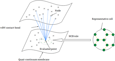
Motivated by the virtual internal bond model proposed by Gao and Klein [Reference Gao and Klein35], we develop a van der Waals (vdW) contact-bond model, where the vdW interactions of nonbonded atoms in the atomic system are simulated by contact bonds between the evaluated points and nodes to take into account the discreteness of the nanoscale components. Compared with the atomistic-based simulations, the established vdW contact-bond model is more effective and efficient in predicting large deformations of nano-structures where the contact behaviors cannot be neglected. The amount of contact bonds can be selected freely for different contact problems. Besides, the computational efforts can, therefore, be significantly reduced, which is particularly attractive in engineering applications. In the higher-order QC model, the geometrically consistent higher-order Cauchy–Born (HCB) rule proposed by Guo et al. [Reference Guo, Wang and Zhang23] is applied to construct the atomic-scale constitutive model. The HCB rule bridges the deformation between the atomic structures and the corresponding equivalent continuum membrane. Many successful applications of the QC model for graphene, nanotubes, nanocones, erythrocyte, microtubules, etc., can be found in Refs. [Reference Guo, Wang and Zhang23, Reference Guo, Liao and Wang24, Reference Wang and Guo25, Reference Sun and Liew26, Reference Wang and Guo27, Reference Wang, Wang and Guo28, Reference Wang, Guo and Su29, Reference Xiang and Liew30]. A variationally consistent meshless computational framework is established based on the developed vdW contact-bond QC model to predict the large deformation of nanoscale carbon components. The meshless local Petrov–Galerkin (MLPG) method [Reference Atluri and Zhu36, Reference Atluri and Zhu37] is resorted to establish a numerical computational framework in which the displacement approximation has higher order continuity. It is a truly meshless method for interpolation and integration purposes, and no additional smoothing technique is required to evaluate the derivatives of the unknown variables.
Interactions between carbon atoms
The interactions between atoms in nanoscale carbon structures include multi-body interatomic potential and pair interatomic potential. Generally, the bond energy of the C–C covalent bond can be described by the multi-body Tersoff–Brenner interatomic potential [Reference Brenner38].
 $$V\left( {{r_{IJ}}} \right) = {V_{\rm{R}}}\left( {{r_{IJ}}} \right) - {\bar{B}_{IJ}}{V_{\rm{A}}}\left( {{r_{IJ}}} \right)\quad ,$$
where r IJ denotes the distance between atoms I and J. V R and V A represent the repulsive and attractive pair terms, respectively.  ${\bar{B}_{IJ}}$ represents the effect of multi-body coupling between bond I–J and other adjacent bonds emanating from atom I. In Eq. (1),
 $${V_{\rm{R}}}\left( r \right) = {{{D^{\left( e \right)}}} \over {S - 1}}{{\rm{e}}^{ - \sqrt {2S} \beta \left[ {r - {R^{\left( e \right)}}} \right]}}{f_{\rm{c}}}\left( r \right)\quad ,$$
 $${V_{\rm{A}}}\left( r \right) = {{{D^{\left( e \right)}}} \over {S - 1}}S{{\rm{e}}^{ - \sqrt {2/S} \beta \left[ {r - {R^{\left( e \right)}}} \right]}}{f_{\rm{c}}}\left( r \right)\quad ,$$
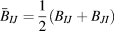 $${\bar{B}_{IJ}} = {1 \over 2}\left( {{B_{IJ}} + {B_{JI}}} \right)$$
with
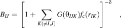 $${B_{IJ}} = {\left[ {1 + \sum\limits_{K\left( { \ne I,J} \right)} {G\left( {{\theta _{IJK}}} \right){f_{\rm{c}}}\left( {{r_{IK}}} \right)} } \right]^{ - \delta }}\quad ,$$
 $$G\left( \theta \right) = {a_0}\left[ {1 + {{c_0^2} \over {d_0^2}} - {{c_0^2} \over {d_0^2 + {{\left( {1 + \cos \;\theta } \right)}^2}}}} \right]\quad ,$$
and θIJK represents the angle between bonds I–J and I–K. f c is a smooth switch function to limit the range of the potential, whose form is usually taken as follows:
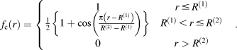 $${f_{\rm{c}}}\left( r \right) = \left\{ {\matrix{ 1 & {r \le {R^{\left( 1 \right)}}} \cr {{1 \over 2}\left\{ {1 + \cos \left( {{{\pi \left( {r\, - \,{R^{\left( 1 \right)}}} \right)} \over {{R^{\left( 2 \right)}}\, - \,{R^{\left( 1 \right)}}}}} \right)} \right\}} & {{R^{\left( 1 \right)}} \lt r \le {R^{\left( 2 \right)}}} \cr 0 & {r > {R^{\left( 2 \right)}}} \cr} \quad .} \right.$$
In this study, the parameters in Eqs. (2)–(7) are set as [Reference Brenner38].
D (e) = 6.000 eV, S = 1.22, β = 21 nm−1, R (e) = 0.1390 nm, δ = 0.50000, a 0 = 0.00020813, c 0 = 330, d 0 = 3.5, R (1) = 0.17 nm, and R (2) = 0.20 nm.
The vdW interatomic interactions between nonbonded carbon atoms can be represented by a pair interatomic potential such as the Lennard–Jones (LJ) potential [Reference Lennard-Jones39].
 $${V_{{\rm{nb}}}} = 4\varepsilon \left[ {{{\left( {{\sigma \over {{r^{{\rm{nb}}}}}}} \right)}^{12}} - {{\left( {{\sigma \over {{r^{{\rm{nb}}}}}}} \right)}^6}} \right]\quad ,$$
where V nb denotes the nonbonded energy between two nonbonded atoms. r nb represents the distance between two nonbonded atoms. ε is the depth of the potential well. σ is the equilibrium distance at which the interatomic interaction potential is zero. In the present study, the values of parameters ε and σ are taken as 2.39 meV and 0.34 nm [Reference Girifalco, Hodak and Lee40], respectively.
The vdW contact-bond model
The constitutive relationship
Compared with the classical CB rule, the HCB rule proposed by Guo et al. [Reference Guo, Wang and Zhang23] for low-dimensional nanocrystalline membranes can enable the mapping of the atomic bonds more accurately. It can account of the curvature effect, which is important for crystalline membranes, in a geometrically consistent way since it involves the second-order or an even more higher-order deformation gradient tensor. The QC constitutive models can involve the information of pair and multi-body interactions of discrete atoms via the HCB rule as an atomic-continuum linkage. Consequently, the HCB rule is appropriate to construct a multiscale QC model for micro/nanoscale materials, including both microstructures and continuum solids. Many studies have shown that the HCB rule, which pulls the membranes more close to the real deformed configurations, can avoid severe numerical instabilities, such as spurious wrinkling [Reference Wang and Guo25, Reference Sun and Liew26, Reference Wang and Guo27, Reference Wang, Wang and Guo28, Reference Wang, Guo and Su29]. The HCB rule can be written as
 $${\bi{r}} = {\bi{F}} \cdot {\bi{R}} + {1 \over 2}{\bi{G}}:\left( {{\bi{R}} \otimes {\bi{R}}} \right)\quad ,$$
where r and R denote the lattice vectors in the deformed and undeformed configurations, respectively. F and G = ∇F are the first- and second-order deformation gradient tensors, respectively, which can be defined by
 $${\bi{F}} = {{\partial {\bi{x}}} \over {\partial {\bi{X}}}},\quad {\bi{G}} = {{{\partial ^2}{\bi{x}}} \over {\partial {\bi{X}} \otimes \partial {\bi{X}}}}\quad ,$$
where X = (X 1, X 2)T is the material coordinate of a point in the reference configuration (i.e., the planar graphene sheet) and x = (x 1, x 2, x 3)T is the image of X in the current configuration. Since the hexagonal crystal lattice of graphene is not centrosymmetrical, in order to guarantee the inner equilibrium of the nano-structure, an inner relaxation parameter η is introduced and the HCB rule is rewritten as
 $${\bi{r}} = {\bi{F}} \cdot \left( {{\bi{R}} + {{\boldeta }}} \right) + {1 \over 2}{\bi{G}}:\left[ {\left( {{\bi{R}} + {{\boldeta }}} \right) \otimes \left( {{\bi{R}} + {{\boldeta }}} \right)} \right]\quad ,$$
where η = (η1, η1)T can be obtained from the energy minimization with respect to η [Reference Guo, Wang and Zhang23].
The strain energy density W 0 of continuum carbon components can be defined as
 $${W_0} = {{\sum\limits_{J = 1}^3 {V\left( {{{\bi{r}}_{IJ}},{{\bi{r}}_{IK}},{\theta _{IJK}},K \ne I,J} \right)} } \over {2{{\rm{\Omega }}_I}}} = {W_0}\left( {{\bi{F}},{\bi{G}},{{\boldeta }}\left( {{\bi{F}},{\bi{G}}} \right)} \right)\quad ,$$
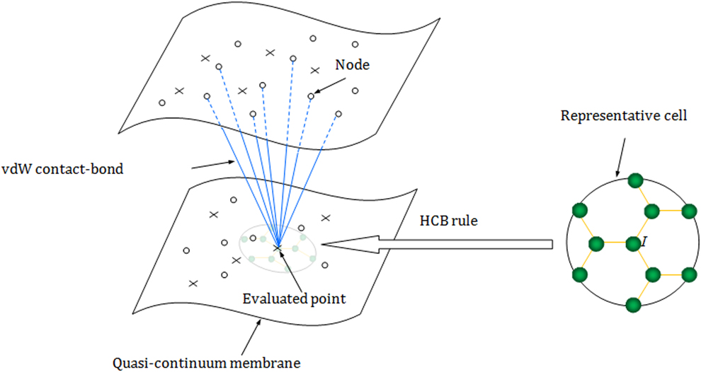
where V is the Tersoff–Brenner potential energy stored in the representative cell, and ΩI is the average area of atom I in the reference configuration (see Fig. 1 for reference).
Illustration of the surface–surface interaction for the wall of CNTs.
From Eq. (12), the first Piola–Kirchhoff stress tensor P and the higher-order stress tensor Q can be derived as
 $${\bi{P}} = {{\partial {W_0}} \over {\partial {\bi{F}}}}\quad ,$$
 $${\bi{Q}} = {{\partial {W_0}} \over {\partial {\bi{G}}}}\quad .$$
Since
 $${{{\partial ^2}{W_0}} \over {\partial {{\boldeta }} \otimes \partial {\bi{F}}}} + {{{\partial ^2}{W_0}} \over {\partial {{\boldeta }} \otimes \partial {{\boldeta }}}} \cdot {{\partial {{\boldeta }}} \over {\partial {\bi{F}}}} = 0\quad ,$$
the tangent modulus tensors can be given as follows:
 $$\scale91%{{{\bi{M}}^{{\rm{FF}}}} = {\left. {{{{\partial ^2}{W_0}} \over {\partial {\bi{F}} \otimes \partial {\bi{F}}}}} \right|_{{{\boldeta }} = {{\hat{\boldeta }}}}} - {\left. {\left[ {{{{\partial ^2}{W_0}} \over {\partial {\bi{F}} \otimes \partial {{\boldeta }}}} \cdot {{\left( {{{{\partial ^2}{W_0}} \over {\partial {{\boldeta }} \otimes \partial {{\boldeta }}}}} \right)}^{ - 1}} \cdot {{{\partial ^2}{W_0}} \over {\partial {{\boldeta }} \otimes \partial {\bi{F}}}}} \right]} \right|_{{{\boldeta }} = {{\hat{\boldeta }}}}}\quad ,$$
 $$\scale89%{{{\bi{M}}^{{\rm{FG}}}} = {\left. {{{{\partial ^2}{W_0}} \over {\partial {\bi{F}} \otimes \partial {\bi{G}}}}} \right|_{{{\boldeta }} = {{\hat{\boldeta }}}}} - {\left. {\left[ {{{{\partial ^2}{W_0}} \over {\partial {\bi{F}} \otimes \partial {{\boldeta }}}} \cdot {{\left( {{{{\partial ^2}{W_0}} \over {\partial {{\boldeta }} \otimes \partial {{\boldeta }}}}} \right)}^{ - 1}} \cdot {{{\partial ^2}{W_0}} \over {\partial {{\boldeta }} \otimes \partial G}}} \right]} \right|_{{{\boldeta }} = {{\hat{\boldeta }}}}}\quad ,$$
 $$\scale89%{{{\bi{M}}^{{\rm{GF}}}} = {\left. {{{{\partial ^2}{W_0}} \over {\partial {\bi{G}} \otimes \partial {\bi{F}}}}} \right|_{{{\boldeta }} = {{\hat{\boldeta }}}}} - {\left. {\left[ {{{{\partial ^2}{W_0}} \over {\partial {\bi{G}} \otimes \partial {{\boldeta }}}} \cdot {{\left( {{{{\partial ^2}{W_0}} \over {\partial {{\boldeta }} \otimes \partial {{\boldeta }}}}} \right)}^{ - 1}} \cdot {{{\partial ^2}{W_0}} \over {\partial {{\boldeta }} \otimes \partial {\bi{F}}}}} \right]} \right|_{{{\boldeta }} = {{\hat{\boldeta }}}}}\quad .$$
 $$\scale89%{{{\bi{M}}^{{\rm{GG}}}} = {\left. {{{{\partial ^2}{W_0}} \over {\partial {\bi{G}} \otimes \partial {\bi{G}}}}} \right|_{{{\boldeta }} = {{\hat{\boldeta }}}}} - {\left. {\left[ {{{{\partial ^2}{W_0}} \over {\partial {\bi{G}} \otimes \partial {{\boldeta }}}} \cdot {{\left( {{{{\partial ^2}{W_0}} \over {\partial {{\boldeta }} \otimes \partial {{\boldeta }}}}} \right)}^{ - 1}} \cdot {{{\partial ^2}{W_0}} \over {\partial {{\boldeta }} \otimes \partial {\bi{G}}}}} \right]} \right|_{{{\boldeta }} = {{\hat{\boldeta }}}}}\quad ,$$
where  ${{\hat{\boldeta }}}$ is the equilibrium solution of η given by
 $${{\partial {W_0}} \over {\partial {{\boldeta }}}} = 0\quad .$$
For explicit expressions of the terms in the above equations, interested readers can refer to Guo et al. [Reference Guo, Wang and Zhang23].
The vdW contact-bond model for point–surface contact
In this section, the vdW contact-bond model is proposed in the higher-order QC theoretical framework for the contact problems of a single carbon atom with a graphene sheet. In order to take into account the discreteness of the interactions of nonbonded atoms in the context of the QC method, the positions of atoms in the discrete nanoscale structure is equivalently replaced by the positions of nodes scattered on the surface of the continuum counterpart. The pair potential energy is assumed to be stored in the virtual bond between two neighbor nodes. A multiscale QC method based on the HCB rule is developed for low-dimensional nanoscale carbon components, and the information of atomic structures can be taken into account via the HCB rule.
The van der Waals (vdW) interaction between a single carbon atom  $\bar{y}$ and a square graphene sheet is characterized by the LJ pair potential. The equivalent QC membrane for this atomistic system is divided by n discrete nodes independent of the number of carbon atoms, and the vdW energy V nb of the system is given by
 $${V_{{\rm{nb}}}}\left( {{r^{{\rm{nb}}}}} \right) = 4{\kappa _0}\varepsilon \sum\limits_{I = 1}^\nu {\left[ {{{\left( {{\sigma \over {r_I^{{\rm{nb}}}}}} \right)}^{12}} - {{\left( {{\sigma \over {r_I^{{\rm{nb}}}}}} \right)}^6}} \right]} \quad ,$$
where the parameter  ${\kappa _0} = {{{A_0}} \over {{\Omega _0}}}$, in which A 0 denotes the area occupied by a node in the QC membrane and Ω0 represents the area divided up evenly to an atom in the graphene sheet.
 $r_I^{{\rm{nb}}}$ is the I-th vdW contact-bond length which can be described as a function of the position of node I, i.e.,
 $r_I^{{\rm{nb}}} = \left| {{{\bi{x}}_I} - \bar{y}} \right|$, where xI = (x I1, x I2, x I3)T and
 $\bar{y} = {\left( {{{\bar{y}}_1},{{\bar{y}}_2},{{\bar{y}}_3}} \right)^T}$ is the position of the single atom. n ≤ N represents the number of contact bonds, which can be chosen freely based on the particularity of problems, such as for the case that the distance of the vdW interaction is relatively large (≥0.85 nm), and n is taken as zero.
The total energy of the atomic system can be written as
 $${E_{{\rm{tot}}}} = {V_{{\mathop{\rm int}} }} + {V_{{\rm{nb}}}} + {V_{{\rm{ext}}}}\quad ,$$
where
 $${V_{{\mathop{\rm int}} }} = \int_\Omega {{W_0}\left( {{\bi{F}},{\bi{G}}} \right){\rm{d}}\Omega }$$
is the internal energy of the QC membrane obtained via the HCB rule as the bridge of the deformation between the atomic structure and the equivalent continuum membrane, and
 $${V_{{\rm{ext}}}} = - \int_\Omega {{{\bi{b}}_0} \cdot {\bi{u}}{\rm{d}}\Omega } - \int_{{\Gamma _t}} {{\bi{t}}_0^P \cdot {\bi{u}}{\rm{d}}S} - \int_{{\Gamma _t}} {{\bi{t}}_0^Q \cdot {\nabla _N}{\bi{u}}{\rm{d}}S}$$
is the external potential (if there is any) of the body force density b0, boundary traction  ${\bi{t}}_0^P$, and boundary couple
 $t_0^Q$.
The equilibrium configuration of solids corresponds to a state of energy minimization, which can be described by the consistent variation of the E tot in Eq. (22) with respect to displacement u as
 $$\delta {E_{{\rm{tot}}}}\left( {{\bi{u}};\delta {\bi{u}}} \right) = \delta {V_{{\mathop{\rm int}} }}\left( {{\bi{u}};\delta {\bi{u}}} \right) + \delta {V_{{\rm{nb}}}}\left( {{\bi{u}};\delta {\bi{u}}} \right) + \delta {V_{{\rm{ext}}}}\left( {\delta {\bi{u}}} \right) = 0\quad ,$$
with the condition δ2E tot > 0. In the continuum meshless numerical framework, u can be interpolated by the moving least square (MLS) approximation [Reference Lancaster and Salkauskas41] as
 $${\bi{u}} = \sum\limits_{I = 1}^N {{\phi _I}\left( {\bi{X}} \right){\bi{u}}_I^ * } \quad ,$$
where N is the total number of nodes in the influence domain,  ${\bi{u}}_I^*$ denotes the displacement parameter of the I-th node, and ϕI(X) is the corresponding meshless shape function, which is expressed by
 $${\phi _I}\left( {\bi{X}} \right) = {\bi{p}}\left( {\bi{X}} \right) \cdot {\left[ {{{\bi{A}}^{ - 1}}\left( {\bi{X}} \right) \cdot {\bi{B}}\left( {\bi{X}} \right)} \right]_I}\quad ,$$
in which p(X) is a full polynomial, and
 $${\bi{A}}\left( {\bi{X}} \right) = \sum\limits_{I = 1}^N {\omega \left( {{\bi{X}} - {{\bi{X}}_I}} \right){\bi{p}}\left( {{{\bi{X}}_I}} \right) \cdot {\bi{p}}\left( {{{\bi{X}}_I}} \right)\quad ,}$$
 $$\scale88%{{\bi{B}}\left( {\bi{X}} \right) = \left[ {\omega \left( {{\bi{X}} - {{\bi{X}}_1}} \right){\bi{p}}\left( {{{\bi{X}}_1}} \right),\;\omega \left( {{\bi{X}} - {{\bi{X}}_2}} \right){\bi{p}}\left( {{{\bi{X}}_2}} \right), \ldots ,\omega \left( {{\bi{X}} - {{\bi{X}}_N}} \right){\bi{p}}\left( {{{\bi{X}}_N}} \right)} \right]\quad ,$$
where ω(X − XI) is the weight function; in this study, the cubic spline function is used as ω.
This carbon atomic system is nonlinear in nature; by substituting Eq. (26) into Eq. (25) and linearizing this virtual work representation, it yields the following incremental governing equation:
 $${\bi{K}}\left( {{{\bi{u}}^n}} \right)\Delta {\bi{u}} = {\bi{f}}\left( {{{\bi{u}}^n}} \right)\quad ,$$
where un denotes the displacement of the n-th step iteration, Δu represents the displacement increment, K is the stiffness matrix given by
 $${K_{\alpha i\beta j}} = {{{\partial ^2}{V_{{\mathop{\rm int}} }}} \over {\partial u_{\alpha i}^*\partial u_{\beta j}^*}} + {{{\partial ^2}{V_{{\rm{nb}}}}} \over {\partial u_{\alpha i}^*\partial u_{\beta j}^*}}\quad ,$$
and f is the nonequilibrium force vector given by
 $${f_{\alpha i}} = - {{\partial {V_{{\mathop{\rm int}} }}} \over {\partial u_{\alpha i}^*}} - {{\partial {V_{{\rm{nb}}}}} \over {\partial u_{\alpha i}^*}} - {{\partial {V_{{\rm{ext}}}}} \over {\partial u_{\alpha i}^*}}\quad ,$$
in which
 $$\displaylines{ {{{\partial ^2}{V_{{\mathop{\rm int}} }}} \over {\partial u_{\alpha i}^*\partial u_{\beta j}^*}} = \int_\Omega {M_{iKjL}^{{\rm{FF}}}{\phi _{\alpha ,K}}{\phi _{\beta ,L}} + M_{iKjLM}^{{\rm{FG}}}{\phi _{\alpha ,K}}{\phi _{\beta ,LM}} + M_{iKLjM}^{{\rm{GF}}}{\phi _{\alpha ,KL}}{\phi _{\beta ,M}}} \cr + M_{iKLjMN}^{{\rm{GG}}}{\phi _{\alpha ,KL}}{\phi _{\beta ,MN}}{\rm{d}}\Omega\quad, \cr} (33)$$
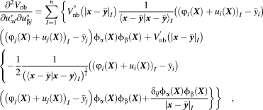 $$\scale89%{\eqalign{ & {{{\partial ^2}{V_{{\rm{nb}}}}} \over {\partial u_{\alpha i}^*\partial u_{\beta j}^*}} = \sum\limits_{I = 1}^n {\left\{ {V_{{\rm{nb}}}^{''}\left( {{{\left| {{\bi{x}} - {{\bar{\bi y}}}} \right|}_I}} \right){1 \over {{{\left\langle {{\bi{x}} - {{\bar{\bi y}}}}|{\bi{x}} - {{\bar{\bi y}}}}} \right\rangle }_I}}}} \right.} \left( {{{\left( {{\varphi _i}\left( {\bi{X}} \right) + {u_i}\left( {\bi{X}} \right)} \right)}_I} - {{\bar{y}}_i}} \right) \cr & \left( {{{\left( {{\varphi _j}\left( {\bi{X}} \right) + {u_j}\left( {\bi{X}} \right)} \right)}_I} - {{\bar{y}}_j}} \right){\phi _\alpha }\left( {\bi{X}} \right){\phi _\beta }\left( {\bi{X}} \right) + V_{{\rm{nb}}}^'\left( {{{\left| {{\bi{x}} - {{\bar{\bi y}}}}} \right|}_I}} \right) \cr & \left\{ { - {1 \over 2}{1 \over {{{\left( {{{\left\langle {{\bi{x}} - {{\bar{\bi y}}}}{\rm{|}}{\bi{x}} - {\bi{y}}} \right\rangle }_I}} \right)}^{{3 \over 2}}}}}} \right.\left( {{{\left( {{\varphi _i}\left( {\bi{X}} \right) + {u_i}\left( {\bi{X}} \right)} \right)}_I} - {{\bar{y}}_i}} \right) \cr & \left( {{{\left( {{\varphi _j}\left( {\bi{X}} \right) + {u_j}\left( {\bi{X}} \right)} \right)}_I} - {{\bar{y}}_j}} \right){\phi _\alpha }\left( {\bi{X}} \right){\phi _\beta }\left( {\bi{X}} \right)\left. {\left. { + {{{\delta _{ij}}{\phi _\alpha }\left( {\bi{X}} \right){\phi _\beta }\left( {\bi{X}} \right)} \over {{{\left| {{\bi{x}} - {{\bar{\bi y}}}}} \right|}_I}}}} \right\}} \right\}\quad , \cr}$$
 $${{\partial {V_{{\mathop{\rm int}} }}} \over {\partial u_{\alpha i}^*}} = \int_\Omega {{P_{iM}}{\phi _{\alpha ,M}} + {Q_{iMN}}{\phi _{\alpha ,MN}}{\rm{d}}\Omega } \quad ,$$
 $$\scale88%{{{\partial {V_{{\rm{nb}}}}} \over {\partial u_{\alpha i}^*}} = \sum\limits_{I = 1}^n {\left( {V_{{\rm{nb}}}^'\left( {{{\left| {{\bi{x}} - {{\bar{\bi y}}}}} \right|}_I}} \right){1 \over {{{\left| {{\bi{x}} - {{\bar{\bi y}}}}} \right|}_I}}}\left( {{{\left( {{\varphi _i}\left( {\bi{X}} \right) + {u_i}\left( {\bi{X}} \right)} \right)}_I} - {{\bar{y}}_i}} \right){\phi _\alpha }\left( {\bi{X}} \right)} \right)\quad ,}$$
 $${{\partial {V_{{\rm{ext}}}}} \over {\partial u_{\alpha i}^*}} = \int_\Omega {{b_{0i}}{\phi _\alpha }d\Omega } + \int_{{\Gamma _t}} {t_{0i}^P{\phi _\alpha } + t_{0i}^Q{N_M}{\phi _{\alpha ,M}}{\rm{d}}S} \quad ,$$
where φ is the mapping from the graphene sheet to the undeformed nanotube.
The vdW contact-bond model for surface–surface contact
The vdW contact-bond model for surface–surface contact problems has higher complexity than the model proposed earlier for the point–surface contact. The vdW interactions of two adjacent carbon crystalline membranes are shown in Fig. 1. The vdW energy V nb between an evaluated point and discrete nodes is given as
 $${V_{{\rm{nb}}}}\left( {{r^{{\rm{nb}}}}} \right) = 4{\kappa _0}{\kappa _1}\varepsilon \sum\limits_{I = 1}^n {\left[ {{{\left( {{\sigma \over {r_I^{{\rm{nb}}}}}} \right)}^{12}} - {{\left( {{\sigma \over {r_I^{{\rm{nb}}}}}} \right)}^6}} \right]} \quad ,$$
where  ${\kappa _1} = {{{A_1}} \over {{\Omega _0}}}$, in which A 1 is the area occupied by the evaluated point, such as the Gaussian quadrature point for the meshless numerical simulation in the following section. The total vdW energy of the system via Eq. (38) is
 $$V_{{\rm{nb}}}^{{\rm{tot}}} = {1 \over 2}\int_\Omega {{{{V_{{\rm{nb}}}}\left( {{r^{{\rm{nb}}}}} \right)} \over {{\Omega _0}}}{\rm{d}}V} \quad .$$
As shown in the following calculations, a small number of contact bonds can guarantee the accuracy of the numerical simulation. It is, therefore, much faster than other existing continuum methods where the vdW energy is represented by [Reference Arroyo and Belytschko33, Reference Wang and Guo34].
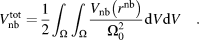 $$V_{{\rm{nb}}}^{{\rm{tot}}} = {1 \over 2}\int_\Omega {\int_\Omega {{{{V_{{\rm{nb}}}}\left( {{r^{{\rm{nb}}}}} \right)} \over {\Omega _0^2}}{\rm{d}}V{\rm{d}}V\quad .} }$$
It is a double integral function, and the computation requires a double loop over the domain Ω. Its numerical computational effort increases with the square of the system size such that these continuum methods are not suitable for large-scale atomic systems.
The vdW interactions depend only on the distance between discrete atoms, which are replaced by single nodes in the contact-bond model. Unlike the homogenization operation of vdW interactions in the continuum methods, the interactions between discrete evaluated points (nodes/quadrature points) in one film and those in another film are described exactly, which ensures the accuracy of this method. Contrary to the atomistic simulations, the proposed contact-bond–based QC method can significantly reduce the degree of freedom of the components and decrease the computation scale, which enables rapid evaluation of large-scale problems.
The first- and second-order derivatives of the vdW energy in Eq. (39) with respect to displacement u for a nonequivalent force vector and stiffness matrix in the governing Eq. (21), respectively, are
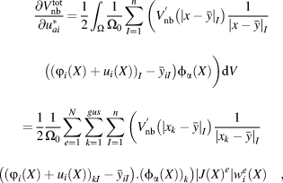 $$& {{\partial V_{{\rm{nb}}}^{{\rm{tot}}}} \over {\partial u_{ai}^*}} = {1 \over 2}\int_\Omega {{1 \over {{\Omega _0}}}} \sum\limits_{I = 1}^n {\left( {V_{{\rm{nb}}}^'\left( {{{\left| {x - \bar{y}} \right|}_I}} \right){1 \over {{{\left| {x - \bar{y}} \right|}_I}}}\left( {{{\left( {{\varphi _i}\left( X \right) + {u_i}\left( X \right)} \right)}_I} - {{\bar{y}}_{iI}}} \right){\phi _\alpha }\left( X \right)} \right\bigg)} {\rm{d}}V & = {1 \over 2}{1 \over {{\Omega _0}}}\sum\limits_{e = 1}^N {\sum\limits_{k = 1}^{gus} {\sum\limits_{I = 1}^n {\left( {V_{{\rm{nb}}}^'\left( {{{\left| {{x_k} - \bar{y}} \right|}_I}} \right){1 \over {{{\left| {{x_k} - \bar{y}} \right|}_I}}}\left( {{{\left( {{\varphi _i}\left( X \right) + {u_i}\left( X \right)} \right)}_{kI}} - {{\bar{y}}_{iI}}} \right)} \right.} } } \cr & \left. {{{\left( {{\phi _\alpha }\left( X \right)} \right)}_k}} \right)\left| {J{{\left( X \right)}^e}} \right|w_i^e\left( X \right)\quad , \cr}$$
 $$\displaylines{ {{{\partial ^2}V_{{\rm{nb}}}^{{\rm{tot}}}} \over {\partial u_{\alpha i}^*\partial u_{\beta j}^*}} = {1 \over 2}{1 \over {{\Omega _0}}}\int_\Omega {\sum\limits_{I = 1}^n {\left[ {V_{{\rm{nb}}}^{''}\left( {{{\left| {x - \bar{y}} \right|}_I}} \right){1 \over {{{\left\langle {x - y|x - y} \right\rangle }_I}}}\left( {{{\left( {{φ _i}\left( X \right) + {u_i}\left( X \right)} \right)}_I} - {{\bar{y}}_{iI}}} \right)} \right} } \cr \left( {{{\left( {{φ _j}\left( X \right) + {u_j}\left( X \right)} \right)}_I} - {{\bar{y}}_{jI}}} \right)\left. {{{{\boldphi }}_\alpha }\left( X \right){{{\boldphi }}_\beta }\left( X \right)} \right\Bigg] + \sum\limits_{I = 1}^n {\left\{ {V_{nb}^'\left( {{{\left| {x - \bar{y}} \right|}_I}} \right)} \right.} \cr \left\{ {\left[ { - {1 \over 2}{1 \over {{{\left( {{{\left\langle {x - \bar{y}|x - \bar{y}} \right\rangle }_I}} \right)}^{{3 \over 2}}}}}} \right.} \right.\left( {{{\left( {{φ _i}\left( X \right) + {u_i}\left( X \right)} \right)}_I} - {{\bar{y}}_{iI}}} \right)\left( {{{\left( {{φ _j}\left( X \right) + {u_j}\left( X \right)} \right)}_I}} \right. \cr \left. { - {{\bar{y}}_{jI}}} \right)\left. {{{{\boldphi }}_\alpha }\left( X \right){{{\boldphi }}_\beta }\left( X \right)} \right\Bigg]\left. {\left. { + {{{\delta _{ij}}{{{\boldphi }}_\alpha }\left( X \right){{{\boldphi }}_\beta }\left( X \right)} \over {{{\left| {x - \bar{y}} \right|}_I}}}} \right\Bigg\}} \right\}{\rm{d}}V \cr = {1 \over 2}{1 \over {{\Omega _0}}}\sum\limits_{e = 1}^N {\sum\limits_{k = 1}^{gus} {\sum\limits_{I = 1}^n {\left\{ {\left[ {V_{{\rm{nb}}}^{''}\left( {{{\left| {{x_k} - \bar{y}} \right|}_I}} \right){1 \over {{{\left\langle {{{\bi{x}}_k} - {{\bar{\bi y}}}}|{{\bi{x}}_k} - {{\bar{\bi y}}}}} \right\rangle }_I}}}\left( {{{\left( {{φ _i}\left( {\bi{X}} \right) + {u_i}\left( {\bi{X}} \right)} \right)}_{kI}} - {{\bar{y}}_{iI}}} \right)} \right} \right} } } \cr \left. {\left( {{{\left( {{φ _j}\left( {\bi{X}} \right) + {u_j}\left( {\bi{X}} \right)} \right)}_{kI}} - {{\bar{y}}_{jI}}} \right){{\left( {{{{\boldphi }}_\alpha }\left( {\bi{X}} \right)} \right)}_k}{{\left( {{{{\boldphi }}_\beta }\left( {\bi{X}} \right)} \right)}_k}} \right\bigg] + V_{{\rm{nb}}}^'\left( {{{\left| {{{\bi{x}}_k} - {{\bar{\bi y}}}}} \right|}_I}} \right) \cr \left\{ { - {1 \over 2}{1 \over {{{\left( {{{\left\langle {{{\bi{x}}_k} - {{\bar{\bi y}}}}|{{\bi{x}}_k} - {{\bar{\bi y}}}}} \right\rangle }_I}} \right)}^{{3 \over 2}}}}}\left( {{{\left( {{φ _i}\left( {\bi{X}} \right) + {u_i}\left( {\bi{X}} \right)} \right)}_{kI}} - {{\bar{y}}_{iI}}} \right)\left( {{{\left( {{φ _j}\left( {\bi{X}} \right) + {u_j}\left( {\bi{X}} \right)} \right)}_{kI}} - {{\bar{y}}_{jI}}} \right)} \right \cr \left. {{{\left( {{{{\boldphi }}_\alpha }\left( {\bi{X}} \right)} \right)}_k}{{\left( {{{{\boldphi }}_\beta }\left( {\bi{X}} \right)} \right)}_k} + \left. {{{{\delta _{ij}}{{\left( {{{{\boldphi }}_\alpha }\left( {\bi{X}} \right)} \right)}_k}{{\left( {{\phi _\beta }\left( {\bi{X}} \right)} \right)}_k}} \over {{{\left| {{{\bi{x}}_k} - {{\bar{\bi y}}}}} \right|}_I}}}}\right\Bigg\}\Bigg\} \left| {J{{\left( {\bi{X}} \right)}^e}} \right|w_i^e\left( {\bi{X}} \right)\quad , \cr}$$
where N is the number of nodes, gus denotes the amount of Gaussian quadrature points within each local subdomain Ωs in the following developed meshless computational framework, and n represents the number of contact bonds between adjacent quadrature points and nodes, which is far less than N, ensuring that the computation scale increases almost linearly with the system size N.
Meshless computational scheme
In recent years, the continuum meshless methods have come into a new stage of rapid development. Unlike the conventional finite element method, continuum solids are not divided into a finite number of elements (FEM), and the shape function depends on the discrete nodes in the local influence domain which overlaps with the neighbor ones in space. As a truly meshless method, the MLPG approach [Reference Atluri and Zhu36, Reference Atluri and Zhu37] is naturally more efficient and flexible in dealing with nonlinear boundary value problems than the conventional FEM and element-free Galerkin (EFG) method. In this study, MLPG is applied to construct a meshless computational framework for the contact behaviors of low-dimensional carbon nano-structures. The degree of freedom of the system can be reduced significantly, and its computational efforts are much lower than those of molecular dynamics simulations. It is, therefore, suitable for the computations of technological applications.
As the proposed QC continuum approach for carbon nanoscale components is based on the Tersoff–Brenner potential, which is nonlinear in nature, the equilibrium configurations can be obtained by solving the linearized governing equation iteratively with the Newton–Raphson method. On the contrary, as the order-N 2 approaches involved only the first-order derivative of the total energy, such as the widely used conjugate gradient method in atomistic simulations, the proposed method enables rapid computations for large-scale systems and significantly reduces the computational efforts. It is noted that when nonlinear bifurcation or material softening occurs, the stiffness matrix K usually becomes nonpositive definite. Under this circumstance, the iterative solution converges to a spurious minimal energy state. This nonphysical problem can be remedied by the replacement of the nonpositive definite K with K + γI, in which I is the same order identity matrix and γ is a positive number to ensure the positive definiteness of K + γI [Reference Liu, Huang, Jiang, Qu and Hwang18]. When the iterative solution approaches the real state of minimal energy, K recovers to positive definite.
The routine of the developed approach can be summarized as follows:
(i) Scatter a finite number of nodes in the domain Ω and on the boundary Γ of the system.
(ii) Determine the local sub-domain Ωs and its boundary Γs for each node.
(iii) Loop over all local sub-domain Ωs and Γ to calculate
 ${{{\partial ^2}{V_{{\mathop{\rm int}} }}} \over {\partial {u^*} \otimes \partial {u^*}}}$, ${{\partial {V_{{\mathop{\rm int}} }}} \over {\partial {u^*}}}$, and ${{\partial {V_{{\rm{ext}}}}} \over {\partial {u^*}}}$.
(a) Determine the Gaussian points in Ωs and on Γs.
(b) Loop over all the Gaussian points.
(1) Calculate shape functions φ and their derivatives with respect to X via MLS approximation for the nodes in the influence domain of the Gaussianpoint.
(2) Calculate deformation gradient tensors F and G.
(3) Calculate stress vectors P and Q and tangent modulus tensors MFF, MFG, MGF, and MGG.
(4) Assemble the contributions to K and f.
(c) End the Gaussian point loop.
(iv) End the domain and boundary loop.
(v) Loop over all local sub-domain Ωs to calculate
${{{\partial ^2}{V_{{\rm{nb}}}}} \over {\partial {u^*} \otimes \partial {u^*}}}$ and ${{\partial {V_{{\rm{nb}}}}} \over {\partial {u^*}}}$.(a) Determine the Gaussian points in Ωs.
(b) Loop over all the Gaussian points.
(1) Calculate the r nb with the use of the position of nodes obtained from the (n − 1)-th iteration step.
(2) Calculate shape functions ϕ via MLS approximation for the nodes in the influence domain of one node.
(3) Assemble the contributions to K and f.
(c) End the Gaussian point loop.
(vi) Solve the governing equation K(u n)Δu = f(u n).
(a) K is positive definite?
(b) If no, then take K as K + γI.
(c) If yes, then continue.
(vii) Update the position of nodes.
(viii) Check if the convergence criterion is satisfied.
(a) If no, then go to (iii).
(b) If yes, then go to the next loading step.


From the above implementation, it is observed that this numerical approach is a truly meshless method without any elements used in conventional FEM and EFG. The nonlocal property of the shape function can readily satisfy the higher-order continuity requirement of the hyperelastic constitutive model for low-dimensional carbon nanoscale components based on the HCB rule.
Accuracy of the vdW contact-bond model
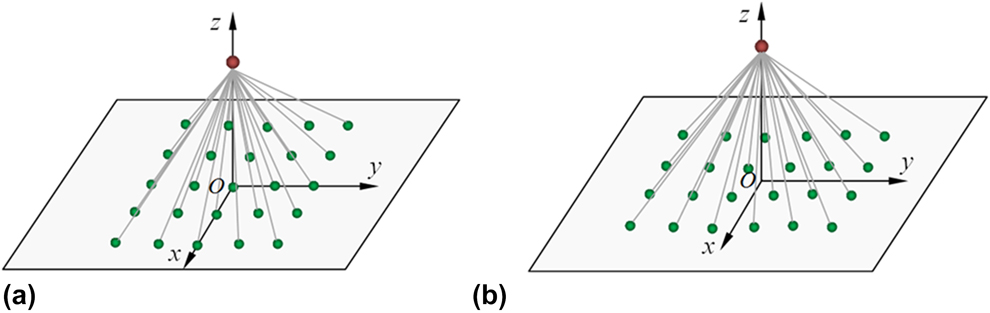
In this section, the accuracy and effectiveness of the vdW contact-bond model for low-dimensional carbon nanoscale contact problems are studied via the following contrast tests. In order to facilitate comparison, two simple examples are illustrated in Fig. 2, namely, point–face (PF) test [Fig. 2(a)] and point–point (PP) test [Fig. 2(b)], respectively. The single carbon atom is 0.6 nm above the 0.8 × 0.8-nm2 square graphene sheet and descends gradually by 0.02 nm per step. The meshless nodes are uniformly scattered on the sheets. In order to exclude the influence of deformation of the graphene sheet for the vdW interactions, the graphene sheet is rigid and fixed. The discrete atomistic model
 $${V_{{\rm{nb}}}} = 4\varepsilon \sum\limits_{I = 1}^n {\left[ {{{\left( {{\sigma \over {r_I^{{\rm{nb}}}}}} \right)}^{12}} - {{\left( {{\sigma \over {r_I^{{\rm{nb}}}}}} \right)}^6}} \right]} \quad ,$$
and the continuum method (homogenization treatment)
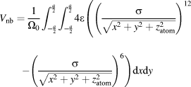 $${V_{{\rm{nb}}}} = {1 \over {{\Omega _0}}}\int_{ - {a \over 2}}^{{a \over 2}} {\int_{ - {a \over 2}}^{{a \over 2}} {4\varepsilon \left( {{{\left( {{\sigma \over {\sqrt {{x^2} + {y^2} + z_{{\rm{atom}}}^2} }}} \right)}^{12}} - {{\left( {{\sigma \over {\sqrt {{x^2} + {y^2} + z_{{\rm{atom}}}^2} }}} \right)}^6}} \Bigg)} } {\rm{d}}x{\rm{d}}y$$
are taken for comparison, where a is the side length of the square graphene sheet, and z atom represents the distance between the carbon atom and the origin of coordinates (square center).
Schematic diagram of the point–surface interaction examples for the (a) PF test and (b) PP test, respectively.
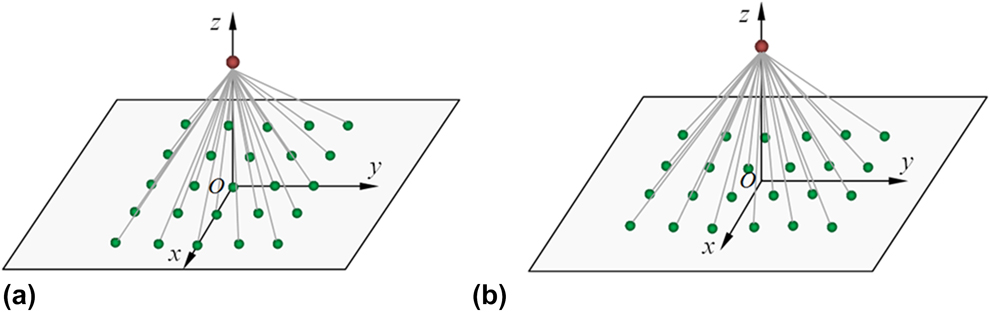
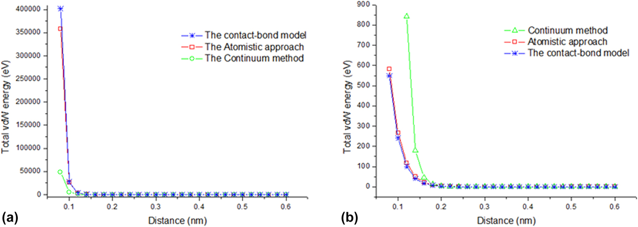
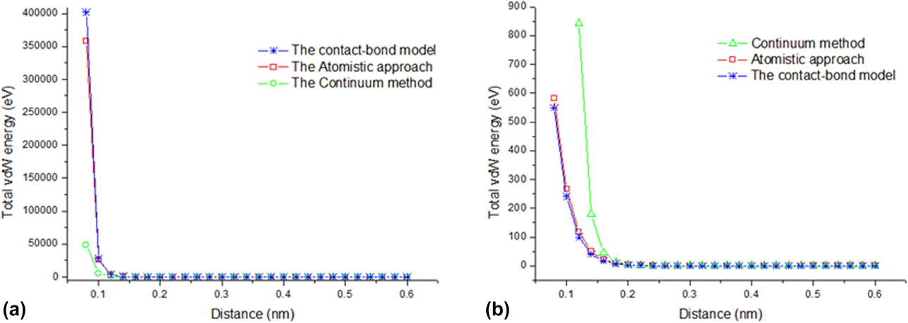
Figure 3 shows the variations of the total vdW energy with respect to the distance between the discrete carbon atom and the graphene sheet for PP and PF tests, respectively, with the usage of the proposed contact-bond model, the atomistic calculation, and the continuum method. It is observed that the vdW energy decreases previously and increases later with the distance between the atom and the sheet reducing, and the turning points for both PP and PF tests appear around the distance of 0.3 nm (the atomistic simulation) and 0.32 nm (the contact-bond model and continuum method). Contrary to atomistic simulation, the continuum results both for PP and PF tests have severe deviation. Although our contact-bond model calculations somewhat underestimate the value of vdW energy when the distance is larger than about 0.26 nm (the vdW interaction is relatively weak), as long as the two components are extremely close, i.e., the distance is less than 0.26 nm, the simulation results of the contact-bond model are in good agreement with the atomistic calculations with an offset of approximately 10%, such as 6.1% for the PP test and 9.9% for the PF test as the distance reaches 0.1 nm.
Variations of the total vdW energy with respect to the distance between the discrete carbon atom and the graphene sheet for the (a) PP test and (b) PF test, respectively.
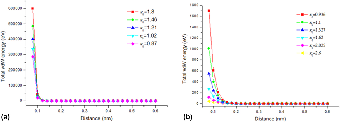
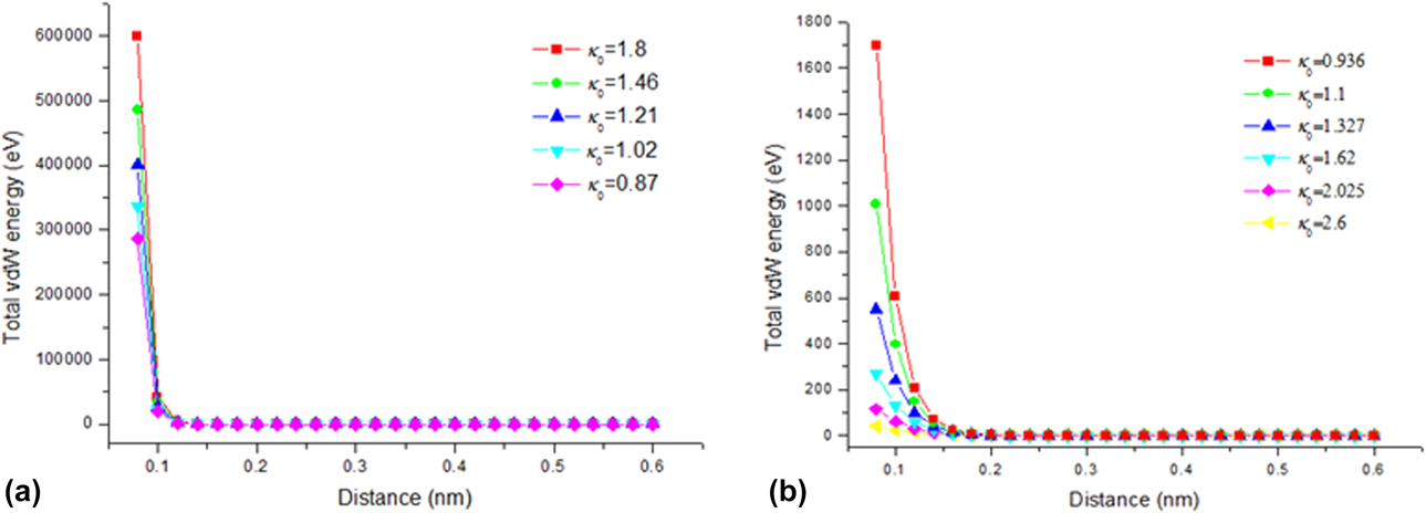
The parameter κ0 in Eq. (21) controlled by the number of meshless nodes has an influence on the vdW interactions simulation with the contact-bond–based QC method, and the results are given in Fig. 4. It is shown that the effect of κ0 on the total vdW energy becomes significant when the distance between the discrete carbon atom and the graphene sheet is less than 0.2 nm. κ0 has an increasing effect on the total vdW energy for the case of the PP test, but has a decreasing effect for the PF test. It can be seen that the value of κ0 taken from about 1.0 to 1.5 can guarantee the consistency of our QC model with the atomistic method.
Influence of parameter κ0 on the total vdW energy for the (a) PP test and (b) PF test.
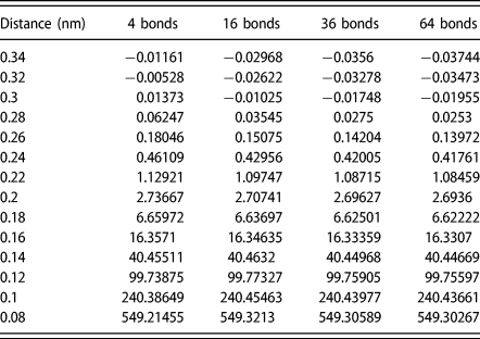
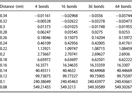
The influence of the number of contact bonds on the vdW interactions is also studied for the PF test, where κ0 = 1.327, and the data are listed in Table I. It indicates that the 4 nearest-neighbor contact bonds play a major role in vdW interactions, and other next nearest-neighbor ones can be neglected, which is conductive to the rapid computation of large-scale systems.
Influence of the number of contact bonds on the total vdW energy (κ0 = 1.327 for the PF test).
From the above discussion, it is obviously observed that the proposed contact-bond model is as accurate as the atomistic simulation, since it involves the equivalently discrete nano-structures which cannot be accounted for in the continuum method. Moreover, the computational efforts can be reduced dramatically as fewer contact bonds are engaged, whereas the accuracy of computation is retained.
Numerical examples and discussion
In order to further demonstrate the proposed contact-bond model and the corresponding QC meshless scheme for the point–surface and surface–surface interactions of low-dimensional nanoscale carbon structures, three different examples are presented in this section.
The first example is for the point–surface contact problem of a single carbon atom and a square graphene sheet. Unlike the example used in the section “Accuracy of the vdW contact-bond model,” only the four sides of a 4 × 4-nm2 graphene sheet are fixed, and displacements of the rest of the domain are not restricted; i.e., the equilibrium configuration of the graphene sheet is determined via energy minimization with the use of the QC meshless scheme. 21 × 21 meshless nodes are used in this numerical simulation (κ0 = 1.37).
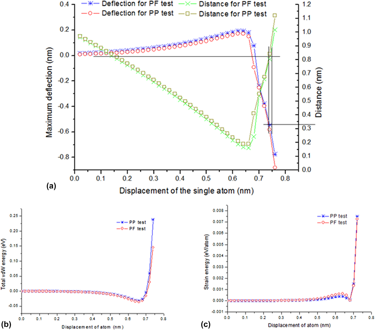
Changes in the maximum deflections of the graphene sheet (the central point deflections) and the distances between the single carbon atom and the graphene sheet with respect to the displacement of the carbon atom are shown in Fig. 5(a). In the initial loading stage (the displacement decreases from 1.0 to 0.64 nm), the upward deflection of the graphene sheet increases gradually, which is captured by the attraction of the vdW interaction. When the displacement is larger than 0.64 nm, the deformation of the graphene sheet is dominated by the repulsive interactions. The total vdW energy obtained from the PP test is larger than that from the PF test, as shown in Fig. 5(b). However, the resultant attractive force contributed by the nearest 4 nodes in the central portion of the graphene sheet in the PF test is larger than that of one node in the center of the graphene sheet in the PP test; the deflections [in Fig. 5(a)] and the strain energy per atom [in Fig. 5(c)] obtained from the PF test are slightly larger than those from the PP test as long as the distance between the atom and the graphene sheet is larger than 0.34 nm. Since the LJ potential increases dramatically when the distance r nb < 0.34 nm, i.e., the distance has a tremendous effect on the vdW interaction (the repulsive interactions playing a dominant role), the contribution of the central node in the graphene sheet to its deflections and strain energy density is larger than that of the surrounding ones. Consequently, the deflections and strain energy density of the graphene sheet obtained in the PP test are larger than that given by the PF test.
(a) Comparison for the maximum deflection of the graphene sheet as well as the distance between the single carbon atom and the graphene sheet under the displacement of the single carbon atom, and the variations of (b) the total vdW energy and (c) the strain energy of the graphene sheet with respect to the displacement of the single carbon atom under two types of loading.
From the above discussion, it is observed that carbon nanoscale point–surface interaction systems can be accurately studied with the proposed contact-bond model. The effectiveness of this method to calculate the nanoscale surface–surface problems for CNTs is illustrated in the following examples.
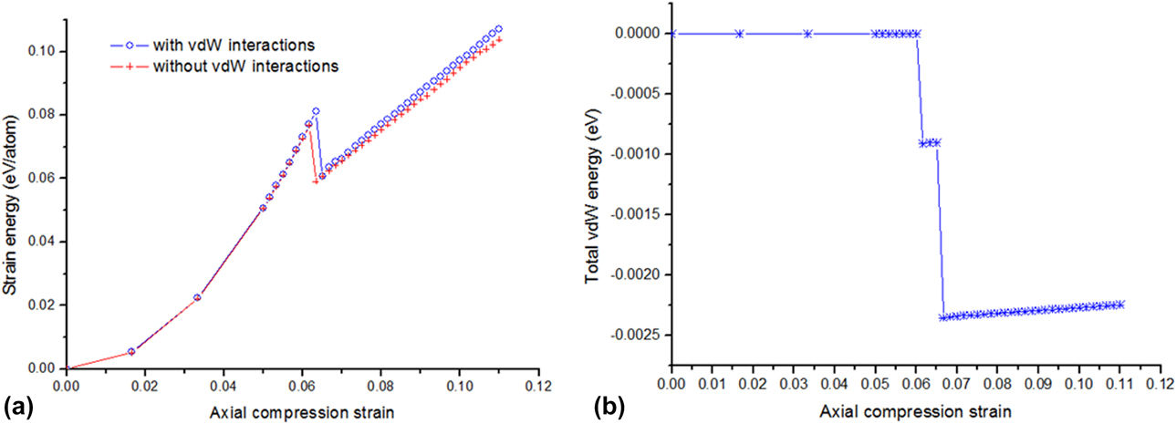
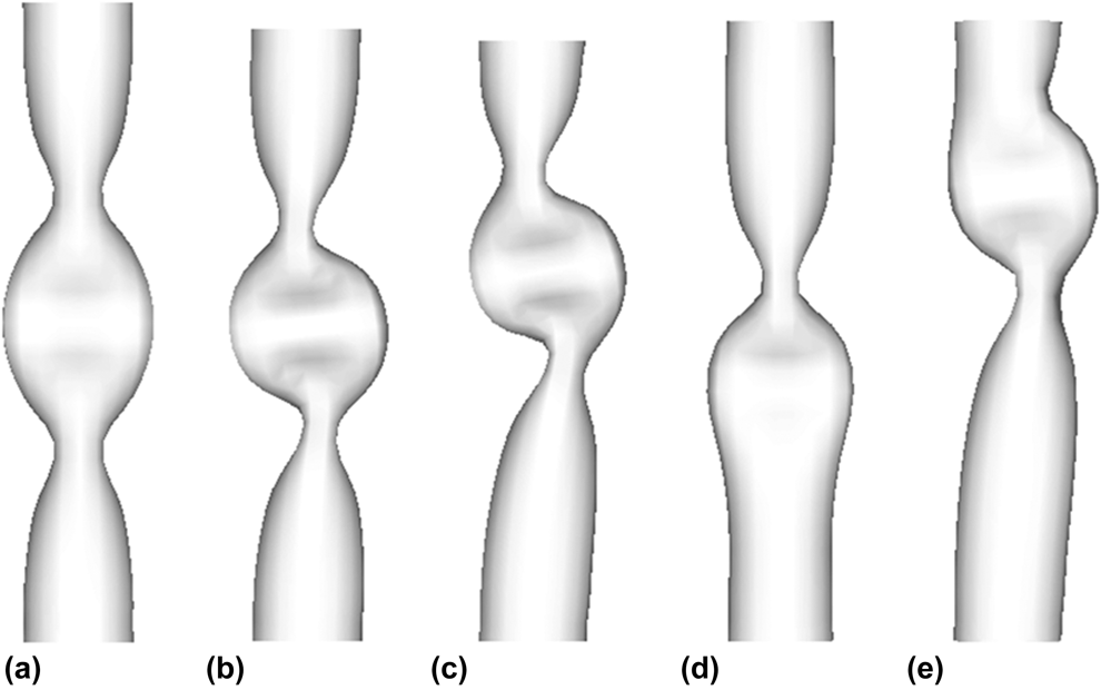
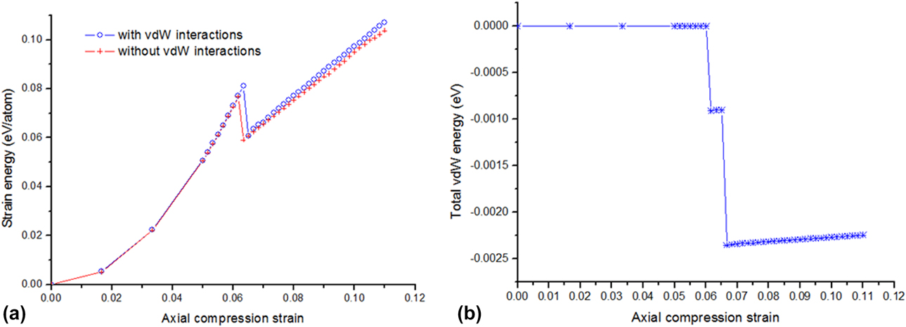
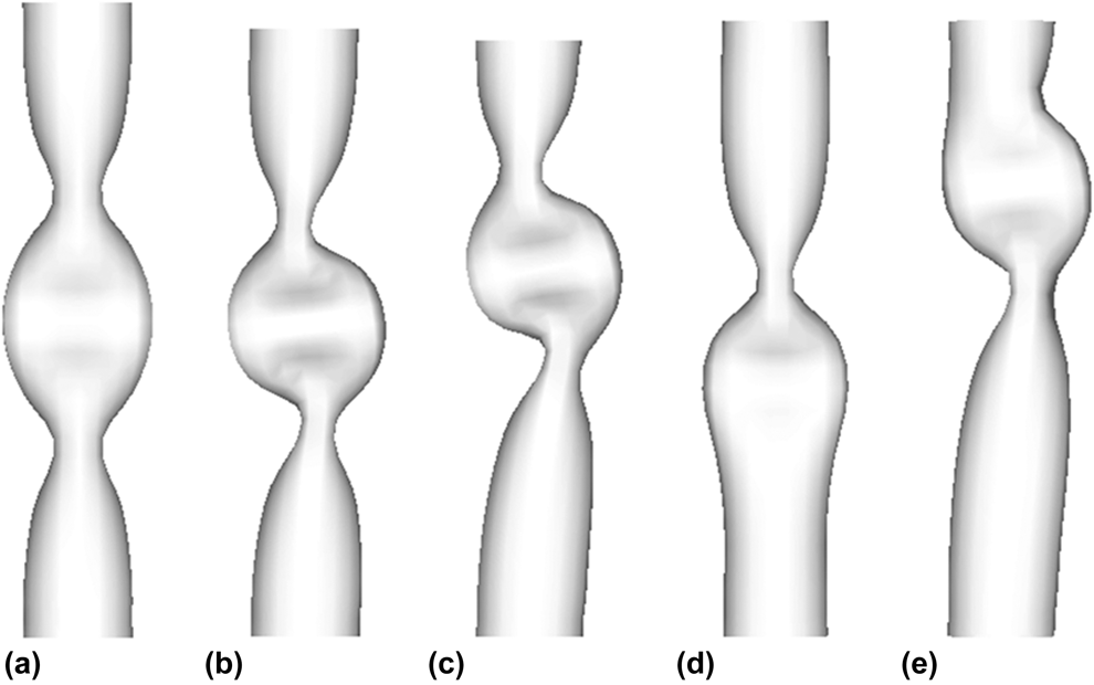
A (7,7) armchair CNT of 6 nm length is selected for the following examination. One end of the nanotube is fixed, and the other end is subjected to axial compression. The number of the meshless nodes is taken as 36 × 18. The variations in strain energy of the (7,7) CNT with respect to the axial compression strain are shown in Fig. 6. For the case of vdW interactions neglected, it can be observed that the first buckling of the SWCNT occurs at the critical strain of 0.062, and the second and third critical buckling strains are 0.09 and 0.105, respectively. This trend agrees well with those reported in [Reference Yakobson, Brabec and Bernholc8] obtained from MD simulations. The corresponding buckling patterns are demonstrated in Figs. 7(a)–7(c). The effect of the vdW interactions on the response of the nanotube are presented in Figs. 6(b), 7(d), and (e). The disturbance due to vdW interactions changes the three-fan buckling pattern of the CNT to the two-fan mode and brings the post-buckling forward from the buckling strain of 0.105 to 0.07.
Changes in (a) the strain energy and (b) the total vdW energy for the CNT under compression with axial strain.
Compression buckling and post-buckling configurations of the (7, 7) CNT without involved vdW interactions at the critical strains of (a) 0.062, (b) 0.09, and (c) 0.105, as well as with involved vdW interactions at the critical strains of (d) 0.063 and (e) 0.07, respectively.
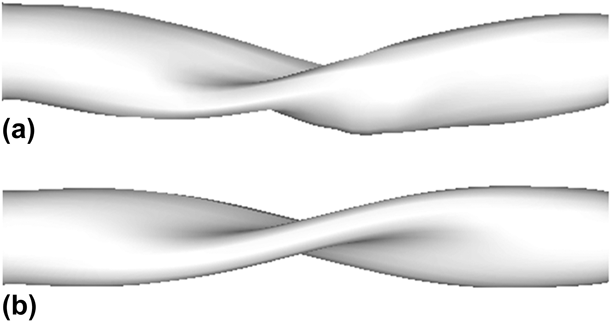
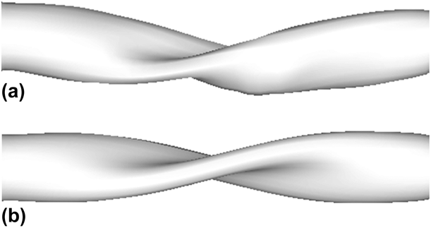
The twisting test of the (21,0) zigzag CNT is also carried out in this section. The tubular length is taken as 11.2 nm, and this nanotube includes 1890 carbon atoms. 58 × 24 meshless nodes are used in the QC meshless numerical simulation. The buckling patterns at different twisting angles are shown in Fig. 8 for the cases of with and without vdW interactions, respectively. From Fig. 8(a), it is observed that the middle portion of the nanotube becomes flat and starts to fold onto itself, which is in good agreement with those reported by Yakobson et al. [Reference Yakobson, Brabec and Bernholc8] and Arroyo and Belytschko [Reference Arroyo and Belytschko33]. The buckling patterns without including the vdW interactions are displayed in Fig. 8(b). It can be seen that the deformation is unphysical and the wall of the nanotube has penetrated itself at a twisting angle of 70°. The computational efforts of this method are far less than that of our previous QC model which double searches the computational domain [Reference Wang and Guo34].
Torsional buckling configurations of the (21, 0) CNT (a) with involved vdW interactions and (b) without involved vdW interactions at the twist angle of 70°, respectively.
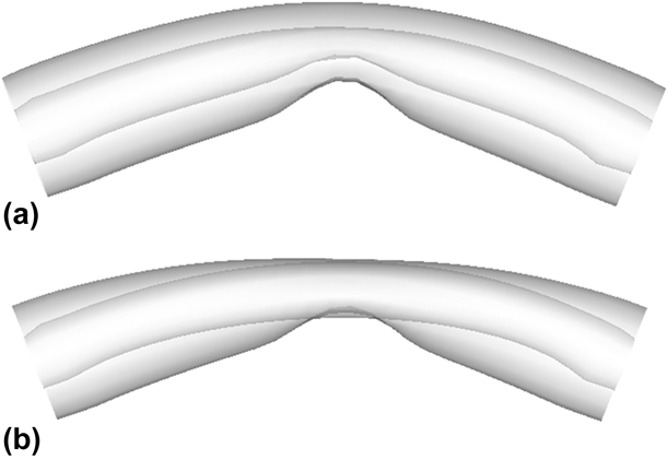
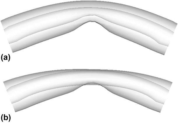
In order to further illustrate the effectiveness of the proposed method, a (6,0) (13,0) double-walled CNT with 5.08 nm length is selected for the numerical bending test. The buckling patterns at 23° bending angle are shown in Fig. 9. It can be seen that the inner tube is also buckling, which is effected by the outer tube through van der Waals interactions [Fig. 9(a)], which is in good agreement with that reported by Iijima et al. [Reference Iijima, Brabec, Maiti and Bernholc42] and Arroyo and Belytschko [Reference Arroyo and Belytschko33]. By contrast, the inner tube is still unbuckling and penetrates the surface of the outer one at the same bending angle [Fig. 9(b)] without considering the contribution of the van der Waals interactions.
Bending buckling patterns of the (6,0) (13,0) double-walled CNT (a) with involved vdW interactions and (b) without involved vdW interactions at the bending angle of 23°, respectively.
As a brief summary, the proposed contact-bond model and the corresponding meshless computational scheme are efficient and accurate for low-dimensional carbon nanoscale contact systems. The degree of freedom for the nanoscale components can be greatly reduced, thus saving the computational efforts. On the other hand, since the HCB rule, which is key to building the QC method, is not limited to a special atomistic model, our method can be expanded to other low-dimensional nanoscale components, such as BN, TiS2, and MoS2 nanotubes.
Concluding remarks
In this study, we have built a van der Waals contact-bond model and proposed a higher-order QC method for the study of the contact behaviors of low-dimensional nanoscale carbon structures. This method takes the multi-body and pair interactions of discrete carbon atoms into account. It is, therefore, as accurate as atomistic simulations. The degree of freedom of the carbon atomic components can be reduced reasonably with the usage of a finite number of nodes to replace the discrete atoms. The saving of computational efforts is tremendous and the computational efficiency is as high as that of continuum simulations. In a nutshell, our method has the advantages of atomistic simulations and continuum models, rendering itself suitable for large-scale problems.
Acknowledgments
We gratefully acknowledge the financial support from the National Natural Science Foundation of China (11602101); the Shandong Provincial Natural Science Foundation for Outstanding Youth, China (ZR2018JL004); and the Promotive Research Fund for Excellent Young and Middle-aged Scientists of Shandong Province, China (BS2014SF004).