












1 Introduction
Helly’s theorem on the intersection of convex sets is one of the most well-known results of combinatorial convexity. Applications, generalizations, and variations of this theorem have been studied extensively for nearly a century, and now comprise a significant area of discrete geometry. We refer the reader to [Reference Danzer, Grünbaum and Klee12, Reference De Loera, Goaoc, Meunier and Mustafa15, Reference Eckhoff19] for in-depth surveys and further references, and to the textbooks [Reference Bárány8, Reference Matoušek36] for an introduction to the area.
1.1 Problem statement
In this paper we are concerned with generalizations of Helly’s theorem that allow for more flexible intersection patterns and relax the convexity assumption.
A central result in this area is the celebrated (p,q)-theorem [Reference Alon and Kleitman4]. It asserts that for a finite family of convex sets in
$\mathbb {R}^d$
 , if the family satisfies the
$(p,q)$
 -condition – meaning that among every p members some q intersect – then a constant number of points suffice to intersect all the convex sets. The crucial feature is that the constant depends only on p, q, and d, but not on the size of the family. Note that Helly’s theorem corresponds to the case
$p=q=d+1$
 , which guarantees that a single point intersects every set in the family.
Two central problems in this line of research are to identify the weakest possible assumptions under which the classical theorems can be generalized, and to determine their key parameters, for instance the Helly number (
$d+1$
 for convex sets in
$\mathbb {R}^d$
 ) or the range for which the
$(p,q)$
 -theorem holds (every
$p \geq q \geq d+1$
 for convex sets in
$\mathbb {R}^d$
 ).
In this paper, we study the
$(p,q)$
 theorem (and other generalizations of Helly’s theorem) in the broad topological setting of triangulable spaces with a forbidden homological minor, a notion introduced by Wagner [Reference Wagner41] as a higher-dimensional analogue of the classical notion of graph minors [Reference Mohar37].
1.2 Our setting
We now describe the general setting in which we establish our
$(p,q)$
 -theorem. Let K be a finite simplicial complex. Throughout this paper, all complexes are assumed to be finite. Homology and chain complexes are taken with
$\mathbb {Z}_2$
 -coefficients, that is,
$C_{{\bullet }}(K)$
 means
$C_{{\bullet }}(K; \mathbb {Z}_2)$
 . We employ singular, simplicial, or cellular homology depending on the context.
Homological minors
Our goal is to establish a
$(p,q)$
 -theorem for a general triangulable space X. It turns out that the key property of the space X we utilize can be deduced from the simplicial complexes that, in a certain sense, do not embed into X. For our purposes, this nonembeddability property is formalized via the concept of a forbidden homological minor, which we now define.
The support of a chain
$\sigma $
 , denoted
$\operatorname {\mathrm {supp}}(\sigma )$
 , in a simplicial complex is the set of simplices with nonzero coefficients in
$\sigma $
 . We say that two chains
$\sigma $
 and
$\tau $
 have overlapping supports if there exists a simplex in the support of
$\sigma $
 that intersects a simplex in the support of
$\tau $
 ; if no such pair of simplices exists we say that
$\sigma $
 and
$\tau $
 have nonoverlapping supports.
A chain map
$f_{\bullet } \colon C_{{\bullet }}(K) \to C_{{\bullet }}(X)$
 is nontrivial if the image of every vertex of K is a
$0$
 -chain of X supported on an odd number of vertices. The simplicial complex K is a homological minor of X, written
${K \prec _H X}$
 , if there exists a nontrivial chain map
$f_{\bullet } \colon C_{{\bullet }}(K) \to C_{{\bullet }}(X)$
 such that disjoint simplices are mapped to chains with nonoverlapping supports. If no such chain map exists we say that K is a forbidden homological minor of X, and write
$K \not \prec _H X$
 . The notion of homological minor readily extends to any triangulable space: K is a forbidden homological minor of a space X if
$K \not \prec _H T$
 for every triangulation T of X.
From now on, rather than focusing on some given space X, we fix a simplicial complex K and consider the entire class of spaces that exclude K as a homological minor. This point of view requires a substitute for the dimension of the ambient space, which turns out to be the parameter

We note the obvious bounds
$\dim K -1 \leq \mu (K) \leq 2\dim K$
 .
Example 1.1. A homological version of Radon’s lemma [Reference Goaoc, Paták, Patáková, Tancer and Wagner21, Lemma 15] asserts that
$\partial \Delta _{d+1} \not \prec _H \mathbb {R}^d$
 , that is, the boundary of the
$(d+1)$
 -dimensional simplex is a forbidden homological minor of
$\mathbb {R}^d$
 . Note that
$\mu \left (\partial \Delta _{d+1}\right ) = d = \dim \partial \Delta _{d+1}$
 . Similarly, a homological version of the Van Kampen-Flores theorem [Reference Goaoc, Paták, Patáková, Tancer and Wagner21, Corollary 14] asserts that
$\Delta _{2k+2}^{(k)}\not \prec _H\mathbb {R}^{2k}$
 , that is, the k-dimensional skeleton of the
$(2k+2)$
 -dimensional simplex is a forbidden homological minor of
$\mathbb {R}^{2k}$
 . Note that
$\mu \left (\Delta _{2k+2}^{(k)}\right ) = 2k = 2\dim \Delta _{2k+2}^{(k)}$
 .
$(K,b)$
 -free covers

Since we have replaced
$\mathbb {R}^d$
 by a general triangulable space X with a forbidden homological minor, the classical notion of a finite family of “convex sets” may no longer be applicable. Therefore, we need to replace and relax the notion of convexity as well.
To this end, let
$\tilde {\beta }_j(\cdot )$
 denote the jth reduced Betti number, that is, the rank of the reduced homology group
$\tilde {H}_j(\cdot )$
 . Given a finite simplicial complex K of positive dimension and a positive integer b we define a (K,b)-free cover in a simplicial complex X to be a finite family
$\mathcal {F}$
 of (not necessarily induced) subcomplexes of X such that:
-
(i) K is a forbidden homological minor of X (i.e., $K\not \prec _H X$
), and -
(ii) the intersection of any nonempty subfamily has bounded complexity:
$$\begin{align*}\tilde{\beta}_j \left( \bigcap_{S\in {\mathcal{G}}}S \right) <b\end{align*}$$for all $0\leq j < \dim K$
and all
$\emptyset \neq \mathcal {G}\subseteq \mathcal {F}$
.


Example 1.2. Let
$K_5$
 denote the complete graph on 5 vertices, viewed as a 1-dimensional simplicial complex, and let X be a triangulation of a
$2$
 -dimensional disk. As a special case of Example 1.1, we have that
$K_5\not \prec _H X$
 .
Illustration: analyzing intersection patterns of planar compact convex sets
Let us showcase how the intersection patterns of finite families of compact convex sets in
$\mathbb {R}^2$
 can be analyzed in our setting.
Consider some finite family
$\mathcal {F}$
 of compact convex sets in
$\mathbb {R}^2$
 . Let X be a sufficiently fine triangulation of the one-point compactification of
$\mathbb {R}^2$
 with the property that any nonempty intersection of members of
$\mathcal {F}$
 contains at least one vertex of X. For each
$S\in \mathcal {F}$
 , let
$C_S$
 denote the subcomplex of X induced by the vertices contained in S, and define
$\mathcal {G} = \{C_S : S\in \cal F\}$
 . Since the sets in
$\mathcal {F}$
 are convex, by choosing X sufficiently fine, we ensure that any nonempty intersection of subcomplexes in
$\cal G$
 is contractible (and thus connected).
On the left: A family of compact convex sets in
$\mathbb {R}^2$
 . On the right: The corresponding
$(K_5,1)$
 -free cover with equivalent intersection pattern.

Figure 1 Long description
The diagram consists of two panels set against a light gray grid background.
On the left panel, five smooth, translucent convex sets are shown in different colors: teal, red, purple, dark blue, and light blue. The teal shape is at the top. The red shape is on the left, overlapping with the teal and dark blue shapes. The purple shape is on the right, overlapping with the teal and dark blue shapes. The dark blue shape is in the center-right, and the light blue shape is at the bottom, overlapping with the dark blue and red shapes. The intersection pattern creates various darker shaded regions where the colors overlap.
On the right panel, the same five shapes are represented as discrete, grid-aligned polygons (K sub 5, 1-free cover). These shapes maintain the same relative positions and intersection patterns as the smooth sets on the left but are composed of blocky, jagged edges that follow the underlying grid. The teal block is at the top, the red block on the left, the purple block on the right, the dark blue block in the center-right, and the light blue block at the bottom. The overlaps between these grid-based shapes mirror the topology of the smooth sets, including a central void where no shapes overlap.
As discussed in Examples 1.1 and 1.2, we have
$K_5\not \prec _H X$
 . Moreover, for every nonempty subfamily
$\mathcal {G'}\subset \mathcal {G}$
 and every
$0\leq j < \dim K_5 = 1$
 , we have

Thus
$\cal G$
 is a
$(K_5, 1)$
 -free cover. Moreover,
$\mathcal {G}$
 has the same intersection pattern as
$\mathcal {F}$
 in the sense that for every integer
$k \ge 1$
 and every subfamily
$\{S_1,S_2, \ldots , S_k\} \subseteq \mathcal {F}$
 , we have

Example 1.3. Every finite family of compact convex sets in
$\mathbb {R}^d$
 is a
$(\partial \Delta _{d+1},1)$
 -free cover. Indeed, by mimicking the previous construction, we obtain a triangulation of the one-point compactification of
$\mathbb {R}^d$
 that preserves intersection patterns; the rest follows from Example 1.1. More generally, every finite good cover – that is, a finite family of open sets in
$\mathbb {R}^d$
 for which every nonempty intersection is contractible – is also a
$(\partial \Delta _{d+1},1)$
 -free cover. Similarly, Example 1.1 implies that every good cover in
$\mathbb {R}^{2k}$
 is also a
$(\Delta _{2k+2}^{(k)}, 1)$
 -free cover.
1.3 Main results
It is known that the Helly number of a
$(K,b)$
 -free cover is bounded from above in terms of K and b [Reference Goaoc, Paták, Patáková, Tancer and Wagner21], as is the Radon number [Reference Patáková39, Proposition 3.7].Footnote
1
This implies that
$(K,b)$
 -free covers also satisfy a fractional Helly theorem [Reference Holmsen and Lee25] and a
$(p,q)$
 -theorem [Reference Alon, Kalai, Matoušek and Meshulam3].
However, this approach yields a
$(p,q)$
 -theorem, but only for
$p\geq q \geq m$
 , where for
$\dim K>1$
 , the threshold m is an extremely large constant derived from successive iterations of Ramsey’s theorem [Reference Patáková39].Footnote
2
Our main result improves this significantly:
Theorem 1.4 (General
$(p,q)$
-theorem)

For every finite simplicial complex K and positive integer b, the
$(p,q)$
 -theorem holds for the class of
$(K,b)$
 -free covers for all
$p\geq q> \mu (K)$
 .
Let us make four remarks:
-
○ It should be clear from the discussion of Section 1.2 that for K the boundary of the $(d+1)$
-simplex and
$b=1$
, Theorem 1.4 already contains the classical
$(p,q)$
-theorem for convex sets in
$\mathbb {R}^d$
. In particular, in that special case the range of pairs
$(p,q)$
is sharp. -
○ Theorem 1.4 implies that for every $p\geq q \geq 3$
and
$b\geq 1$
, the assertion of the
$(p,q)$
-theorem holds for any finite family of sets in the plane, such that the intersection of every subfamily has at most b path-connected components (it is a
$(K_5,b)$
-free cover). This was known before only for open sets and
$b=1$
while for
$b \geq 2$
one had to assume that
$q \geq 2b+2$
[Reference Patáková39]. -
○ The bound on the piercing number given by Theorem 1.4 depends on p, q, K, and b, but is independent of the size of the cover.
-
○ While the Helly number of a $(K,b)$
-free cover can grow with b (it is at least
$b(\mu (K)+2)$
[Reference Goaoc, Paták, Patáková, Tancer and Wagner21, Example 2]), the range for which the
$(p,q)$
-theorem holds is independent of b. This is similar to the gap observed for convex lattice sets (sets of the form
$C\cap \mathbb {Z}^d$
where C is a convex set in
$\mathbb {R}^d$
), which have Helly number
$2^d$
[Reference Doignon17, Reference Scarf40] and satisfy a
$(p,q)$
-theorem for every
$p \geq q \geq d+1$
[Reference Bárány and Matoušek9].


We now describe our main technical result, which serves as the cornerstone of the proof of Theorem 1.4. For a finite family
$\mathcal {F}$
 of subsets of some (finite or infinite) ground set, let
$\pi _m(\mathcal {F})$
 denote the number of m-element subfamilies of
$\mathcal {F}$
 with nonempty intersection.
A straightforward counting argument shows that “positive density propagates downwards” in the sense that if
$\pi _m(\mathcal {F}) \geq \alpha \binom {|\mathcal {F}|}{m}$
 , then
$\pi _{m-1}(\mathcal {F})\geq \alpha \binom {|\mathcal {F}|}{m-1}$
 . (A sharper bound follows from the Kruskal–Katona theorem.) We show that, in essence, positive density propagates upwards for
$(K,b)$
 -free covers:
Theorem 1.5 (Stepping-up theorem)
Fix a simplicial complex K, a real number
$\delta \in (0,1]$
 , and integers
$b\geq 1$
 and
$m> \mu (K)$
 . If
$\mathcal {F}$
 is a sufficiently large
$(K,b)$
 -free cover such that
$\pi _m(\mathcal {F})\geq \delta \binom { | \mathcal {F} | }{m}$
 , then
$\pi _{m+1}(\mathcal {F})\geq \gamma \binom { | \mathcal {F} |}{m+1}$
 , where
$\gamma> 0$
 is a constant depending only on
$\delta $
 , b, m, and K.
One immediate application of Theorem 1.5 is the reduction of fractional Helly numbers. For instance, it easily improves a theorem of Patáková [Reference Patáková39, Theorem 2.3] into:Footnote 3
Theorem 1.6 (Fractional Helly theorem)
Let K be a finite simplicial complex and
$b \geq 1$
 an integer. If a positive fraction of the
$(\mu (K)+1)$
 -tuples of a
$(K,b)$
 -free cover
$\mathcal {F}$
 have nonempty intersection, then there is a subfamily with nonempty intersection containing a positive fraction of the members of
$\mathcal {F}$
 .
In the terminology of combinatorial convexity, Theorem 1.6 states that the fractional Helly number for
$(K,b)$
 -free covers is at most
$\mu (K)+1$
 . Specifically, for any
$\alpha> 0$
 , if a
$(K,b)$
 -free cover
$\mathcal {F}$
 satisfies
$\pi _{\mu (K)+1}(\mathcal {F}) \geq \alpha \binom { | \mathcal {F} |}{\mu (K)+1}$
 , then there exists a subfamily
$\mathcal {G} \subset \mathcal {F}$
 of size at least
$\beta |\mathcal {F}|$
 with nonempty intersection, where
$\beta>0$
 depends only on K, b, and
$\alpha $
 .
Theorem 1.5 generalizes a classical observation for convex sets. Theorems 1.4 and 1.6 generalize and unify a number of results in the area. See Section 7 for further discussion.
2 Proof outline
We now outline the proof of our main results and introduce some necessary terminology. We write
$\mathbb {N} = \{1,2,\ldots \}$
 for the set of positive integers and
$\mathbb {N}_0 = \{0,1,\ldots \}$
 for the set of nonnegative integers. We write
$[n] = \{1,2,\ldots , n\}$
 and
$\binom {[n]}{k}$
 for the set of k-element subsets of
$[n]$
 . For a simplicial (or cell) complex K, we denote by
$K^{(t)}$
 the t-skeleton of K.
2.1 Improving fractional Helly and
$(p,q)$
-theorems using stepping-up

Let us first explain why the stepping-up Theorem 1.5 can be easily combined with the existing literature to yield Theorems 1.4 and 1.6.
Improved fractional Helly from stepping-up
A fractional Helly theorem for
$(K,b)$
 -free covers was previously established by the third author [Reference Patáková39] with a worse fractional Helly number: the assumption is that a positive fraction of the m-tuples have nonempty intersection, where for
$\dim K>1$
 , m is a hypergraph Ramsey number depending on b and K.
To prove Theorem 1.6 it therefore suffices to show that if a positive fraction of the
$(\mu (K)+1)$
 -tuples intersect, then a positive fraction of the m-tuples intersect. This follows from successive applications of Theorem 1.5. (Note that the existence of a finite m established in [Reference Patáková39, Theorem 2.3] is essential to ensure this process terminates; additionally, the implicit bound on
$\beta $
 derived from [Reference Patáková39, Theorem 2.3] changes during this process.)
Improved
$(p,q)$
-theorem from improved fractional Helly

Theorem 1.4 is an immediate consequence of Theorem 1.6 and the results of Alon et al. [Reference Alon, Kalai, Matoušek and Meshulam3]. In essence, Alon et al. show that if an intersection closed set system has fractional Helly number at most m, then the set system also satisfies a
$(p,q)$
 -theorem for the range
$p \geq q \geq m$
 (see Theorems 8(i) and 9 and the discussion in
$\S 2.1$
 in [Reference Alon, Kalai, Matoušek and Meshulam3]). Thus, Theorem 1.4 follows by applying Theorem 1.6 to the intersection closure
$\mathcal {F}^\cap := \{ \cap _{S \in \mathcal {G}} S \colon \mathcal {G} \subset \mathcal {F}\}$
 , observing that
$\mathcal {F}^\cap $
 is a
$(K,b)$
 -free cover if and only if
$\mathcal {F}$
 is.
2.2 Proof outline for the stepping up theorem: reduction to a weak colorful Helly
Let us now turn our attention to our main technical contribution, the stepping-up Theorem 1.5. At a high-level, it is a consequence of a suitable colorful Helly theorem, combined with hypergraph supersaturation. This approach has been successfully applied to various problems in combinatorial geometry; see, for example, [Reference Alon, Bárány, Füredi and Kleitman1], [Reference Bárány8, chapters 23, 29, 33], [Reference Bárány and Matoušek9], [Reference Matoušek36, chapter 9]. We now present its main ingredients.
A hypergraph supersaturation argument
For a more detailed explanation, it is convenient to reformulate the problem in terms of hypergraphs. Given a
$(K,b)$
 -free cover
$\mathcal {F}$
 , we consider a hypergraph
$\mathcal {H}$
 whose vertices correspond to the members of
$\mathcal {F}$
 and whose edges correspond to the intersecting m-tuples in
$\mathcal {F}$
 . This makes
$\mathcal {H}$
 a dense m-uniform hypergraph on
$|\mathcal {F}|$
 vertices and
$\pi _m(\mathcal {F})> \delta \binom {|\mathcal {F}|}{m}$
 edges. The Erdős–Simonovits (supersaturation) theorem [Reference Erdős and Simonovits20] implies that there exist at least
$\rho \binom {|\mathcal {F}|}{mt}$
 distinct vertex subsets of size
$mt$
 that each span a complete m-partite subhypergraph with parts of size t. Here t is any fixed positive integer, and crucially, the fraction
$\rho> 0$
 depends only on m, t, and
$\delta $
 . In other words, the positive edge density of
$\mathcal {H}$
 ensures a positive density of complete m-partite subhypergraphs with parts of size t.
Returning to the
$(K,b)$
 -free cover
$\mathcal {F}$
 , each complete m-partite subhypergraph in
$\mathcal {H}$
 corresponds to a collection of disjoint subfamilies
$\mathcal {F}_1, \dots , \mathcal {F}_m \subset \mathcal {F}$
 , with
$|\mathcal {F}_i| = t$
 , such that
$S_1\cap \cdots \cap S_m\neq \emptyset $
 for every choice
$S_i\in \mathcal {F}_i$
 . This is a familiar intersection pattern originating in the colorful Helly theorem [Reference Bárány7].
Colored
$(K,b)$
-free covers and a weak colorful Helly theorem

This leads us to introduce a colorful analogue of
$(K,b)$
 -free covers. Given a collection of nonempty set systems
$\mathcal {F}_1, \mathcal {F}_2, \ldots , \mathcal {F}_m$
 , a subfamily
$\mathcal {G} \subset \bigcup _{i=1}^m \mathcal {F}_i$
 is called colorful if
$\mathcal {G}$
 contains at most one member from each
$\mathcal {F}_i$
 . We define an m-colored (K,b)-free cover in a simplicial complex X to be a finite family
$\mathcal {F} = \mathcal {F}_1 \sqcup \mathcal {F}_2 \sqcup \cdots \sqcup \mathcal {F}_m$
 of subcomplexes of X such that:
-
(i) K is a forbidden homological minor of X, and
-
(ii) $\tilde {\beta }_j(\bigcap _{S \in \mathcal {G}}S) < b$
for all
$0\leq j < \dim (K)$
and all nonempty colorful subfamilies
$\mathcal {G} \subseteq \mathcal {F}$
.



Returning to the relation between the family
$\mathcal {F}$
 and the m-regular hypergraph
$\mathcal {H}$
 , every subset of
$mt$
 vertices that spans a complete m-partite subhypergraph with parts of size t corresponds to a subfamily of
$\mathcal {F}$
 that can be colored to form an m-colored
$(K,b)$
 -free cover where each color class has size t and every colorful subfamily has nonempty intersection. We prove that each such family has the following property:
Theorem 2.1 (weak colorful Helly theorem)
For any simplicial complex K and integers
$b\geq 1$
 and
$m> \mu (K)$
 , there exists an integer
$t = t(b,K,m)$
 with the following property: If
$\mathcal {F} = \mathcal {F}_1 \sqcup \cdots \sqcup \mathcal {F}_m$
 is an m-colored
$(K,b)$
 -free cover where each color class has size t and every colorful subfamily has nonempty intersection, then
$\mathcal {F}$
 contains some
$2m-\mu (K)$
 members with nonempty intersection.
Note that the definition of colored
$(K,b)$
 -free cover does not impose any condition on the noncolorful subfamilies, as this is not needed for the proof of Theorem 2.1.
Stepping up from weak colorful Helly and supersaturation
Our main result, Theorem 1.5, now follows from Theorem 2.1 via double counting and supersaturation.
Specifically, let
$\mathcal {F}$
 be a
$(K,b)$
 -free cover with at least
$\delta \binom {|\mathcal {F}|}{m}$
 intersecting m-tuples, where
$m> \mu (K)$
 , and let
$t = t(b,K,m)$
 be the integer provided by Theorem 2.1. By the supersaturation argument outlined above, there are at least
$\rho \binom {|\mathcal {F}|}{mt} m$
 -colored subfamilies of
$\mathcal {F}$
 that satisfy the hypothesis of Theorem 2.1.
For each such m-colored subfamily, we apply Theorem 2.1 to find an intersecting subfamily of size
$2m-\mu (K)$
 . Since
$2m-\mu (K) \geq m+1$
 , this implies the existence of an intersecting
$(m+1)$
 -tuple within that subfamily. By summing over all such subfamilies and correcting for the number of times a given intersecting
$(m+1)$
 -tuple is counted, we conclude that there are at least
$\gamma \binom {|\mathcal {F}|}{m+1}$
 intersecting
$(m+1)$
 -tuples, where
$\gamma>0$
 depends only on
$\delta $
 , b, m, and K.
The full details of this argument are provided in Section 6.
2.3 Proof outline for the weak colorful Helly theorem
The proof of Theorem 2.1 is quite involved and builds on the method of constrained chain maps developed in [Reference Goaoc, Paták, Patáková, Tancer and Wagner21, Reference Patáková39]. A major part of this paper, specifically Sections 3, 4, and 5, is devoted to adapt this machinery to handle the m-partite structure of colorful intersection patterns. Here we introduce the key ideas on a simple example, then give some indication of how these ideas can be extended to the general case.
The example
Let us consider a simplified situation where we are given a 3-colored family
$\mathcal {F} = \mathcal {F}_1 \sqcup \mathcal {F}_2 \sqcup \mathcal {F}_3$
 of open connected sets in
$\mathbb {R}^2$
 such that the intersection of any colorful subfamily is nonempty and connected. We show that if
$|\mathcal {F}_i| = 5$
 for every
$1\leq i \leq 3$
 , then there exist four members in
$\mathcal {F}$
 with nonempty intersection.
Encoding the family in a graph
The colorful subfamilies of
$\mathcal {F}$
 are encoded by a graph
$G = (V,E)$
 , defined on the vertex set
$V = \{(a_1,a_2,a_3)\in \mathbb {N}^3 : 1\leq a_i \leq 5\}$
 . Vertices u and v are connected by an edge,
$e = uv$
 , whenever their Euclidean distance satisfies
$|u-v|=1$
 . It is convenient to view G as a 1-dimensional complex realized in
$\mathbb {R}^3$
 with its vertices on the integer lattice, and edges parallel to the coordinate axes, forming a 3-dimensional grid (see Figure 2, left).
On the left: A planar projection of the graph G from the
$[5]\times [5] \times [5]$
 grid in
$\mathbb {Z}^3$
 . The edges of
$K_5$
 are mapped by
$g_{\bullet }$
 to the blue paths. On the right: Connecting points
$p_u$
 and
$p_v$
 by a constrained path
$\gamma _{uv}.$


Figure 2 Long description
The left panel displays a three-dimensional lattice representing a 5 times 5 times 5 grid in Z super 3. Black dots mark the vertices of the grid. Thick blue lines trace specific paths along the edges of the grid, primarily concentrated on the top and left faces of the cube structure. The right panel shows three overlaping sets and a constrained path. The sets are colored red, green and blue, where the blue set has two connected components and intersects both red and green set. Moreover, the intersection of red and green is connected. The vertices of the constrained path are placed at the two distinct connected components of the intersection of all three sets, while the path is fully contained in the intersection of red and green set.
We introduce a map
$\psi $
 that assigns a colorful subfamily of
$\mathcal {F}$
 to every cell (vertex or edge) in G. First, we label the sets in
$\mathcal {F}$
 such that
$\mathcal {F}_j = \{ S_{1,j}, \dots , S_{5,j}\}$
 for
$1\leq j \leq 3$
 . The mapping
$\psi $
 is then defined as follows:
-
For a vertex $v = (a,b,c)$
,
$\psi $
selects one set from each family:
$\psi (v) = \{S_{a,1}, S_{b,2}, S_{c,3}\}$
. -
For an edge $uv$
,
$\psi $
assigns the intersection of the endpoint values:
$\psi (uv) = \psi (u) \cap \psi (v)$
.


Note that
$\psi $
 establishes a bijection between the vertices of G and the maximal colorful subfamilies of
$\mathcal {F}$
 , and for any edge e, we have
$|\psi (e)| = 2$
 . Furthermore, for any two edges e and
$e'$
 , the size
$|\psi (e) \cup \psi (e')|$
 is determined by the relative geometric alignment of e and
$e'$
 in the grid:
-
If e and $e'$
are contained in a common axis-parallel line, then
$\psi (e) = \psi (e')$
, and so
$|\psi (e) \cup \psi (e')| = 2$
. -
If e and $e'$
are contained in a common axis-parallel plane, but not in a common axis-parallel line, then
$\psi (e)$
and
$\psi (e')$
have exactly one member in common, and so
$|\psi (e) \cup \psi (e')| = 3$
.





Most important for us is the following property:
-
If e and $e'$
are not contained in any common axis-parallel plane, then
$\psi (e)$
and
$\psi (e')$
are disjoint, and so
$|\psi (e) \cup \psi (e')| = 4$
.


(Chain) maps
To prove that some four members of
$\mathcal {F}$
 intersect, we construct maps relating
$K_5$
 , G, and
$\mathbb {R}^2$
 . In this simple example, these could be (PL) maps, but it turns out to be convenient in the general case to work with chain maps. We thus use chain maps also for this simple example.

The first chain map
The first is a map
$f_{\bullet } \colon C_{\bullet }(G) \to C_{\bullet }(\mathbb {R}^2)$
 , defined as follows:
-
On vertices (0-chains): For a vertex v in G we select a representative point $p_v \in \mathbb {R}^2$
contained in the common intersection of the sets in
$\psi (v)$
. We set
$f_0(v) = p_v$
. -
On edges (1-chains): Consider an edge $uv$
in G. The points
$p_u$
and
$p_v$
are both contained in the intersection of the subfamily
$\psi (uv)$
. Since this intersection is assumed to be connected, there exists a path
$\gamma _{uv}$
connecting
$p_u$
to
$p_v$
entirely within
$\bigcap _{S\in \psi (uv)}S$
. We set
$f_1(uv) = \gamma _{uv}$
.



The construction of
$f_{\bullet }$
 is completed by extending linearly to arbitrary chains. A key feature of this construction is that for every cell
$\sigma \in G$
 , the image
$f_{\bullet }(\sigma )$
 is contained within the intersection
$\bigcap _{S\in \psi (\sigma )} S$
 . This containment property is what we refer to when we say that
$f_{\bullet }$
 is constrained by the colorful family
$\mathcal {F}$
 (see Figure 2).
The second chain map
We now define the second chain map
$g_{\bullet } \colon K_5 \to G$
 , which sends the vertices
$v_1, \dots , v_5$
 of
$K_5$
 to the vertices
$(1,1,1), \dots , (5,5,5)$
 along the main diagonal in the geometric representation of G. Each edge
$v_iv_j$
 in
$K_5$
 is mapped to a specific path in G connecting the corresponding diagonal vertices. These paths are constructed to satisfy the following crucial geometric property:
-
For any two disjoint edges e and $e'$
in
$K_5$
, if an axis-parallel plane P contains an edge
$\tau $
from the path
$g_1(e)$
, then P does not contain any edge
$\tau '$
from the path
$g_1(e')$
.


We omit the explicit construction of these paths for the moment, referring instead to Figure 2.
The new intersection appears
To find four intersecting members in
$\mathcal {F}$
 , we compose
$f_{\bullet }$
 with
$g_{\bullet }$
 to obtain the chain map
$h_{\bullet } \colon C_{\bullet }(K_5) \to C_{\bullet }(\mathbb {R}^2)$
 as in the diagram above. Because
$K_5$
 is a forbidden homological minor of
$\mathbb {R}^2$
 ,
$h_{\bullet }$
 must result in two disjoint edges e and
$e'$
 in
$K_5$
 whose images
$h_1(e)$
 and
$h_1(e')$
 overlap. Since
$h_{\bullet }$
 factors through
$C_{\bullet }(G)$
 , there must exist specific edges
$\tau $
 from the path
$g_1(e)$
 and
$\tau '$
 from the path
$g_1(e')$
 whose images
$f_1(\tau )$
 and
$f_1(\tau ')$
 intersect at some point
$p\in \mathbb {R}^2$
 . Recalling that
$f_{\bullet }$
 is constrained by
$\mathcal {F}$
 , the point p must lie in the intersection of all the sets in the subfamily
$\psi (\tau ) \cup \psi (\tau ')$
 . By the geometric property highlighted above, these grid edges
$\tau $
 and
$\tau '$
 do not lie in any common axis-parallel plane; thus
$|\psi (\tau ) \cup \psi (\tau ')| = 4$
 . Therefore p is contained in the intersection of four distinct members of
$\mathcal {F}$
 .
Roadmap for the general case
Stepping back, we see that the only property of
$\mathbb {R}^2$
 that we used above was that
$K_5$
 is a forbidden homological minor. In fact, the same argument demonstrates that for
$K = K_5$
 ,
$b=1$
 , and
$m=3$
 , the parameter
$t(b,K,m)$
 in Theorem 2.1 satisfies
$t\leq 5$
 . The proof for general K, b, and m (given in Section 6) follows the same basic structure. Let us highlight the main steps that need to be established along the way:
The grid complex
The colorful subfamilies of
$\mathcal {F}$
 are encoded by a suitable grid complex whose vertices lie on the integer grid
$\mathbb {Z}^m$
 . We introduce the general grid complex
$G[n]^m$
 in Section 3.1, where we also establish terminology and basic properties that will be used throughout the paper. The crucial notion of a subgrid is introduced in Section 3.2, while the encoding of colorful subfamilies via grid complexes is given in Section 3.3.
The first chain map: Constrained chain maps
Our goal is to build chain maps as in the diagram from the proof sketch above, though certain technical obstacles arise that were absent in the simplified setting.
For instance, when
$b>1$
 , the intersection of a colorful subfamily may have several connected components, making it impossible to find a constrained path
$\gamma _{uv}$
 as we did previously. However, since we have an absolute bound on the number of connected components (bounded by b), we can ensure – provided the color classes
$\mathcal {F}_i$
 are sufficiently large – that many of the vertex images lie in the same connected component. This allows us to construct some constrained paths.
Our strategy is to construct enough paths (as well as higher-dimensional chains) to form a sufficiently large subgrid
$G'$
 from which we can construct a chain map
$f_{\bullet } \colon C_{\bullet }(G') \to C_{\bullet }(X)$
 that is constrained by
$\mathcal {F}$
 . This notion is formally defined in Section 4.1.
The existence of such a constrained chain map (Lemma 4.1) is achieved using Ramsey-type arguments – specifically, the Gallai–Witt Theorem [Reference Witt43] on monochromatic subsets of
$\ \mathbb {Z}^m$
 – which we use to establish a vanishing lemma for subgrids in Section 4.2. We then prove the existence of constrained chain maps in Section 4.3.
The second chain map: Generic chain maps into grid complexes
To complete the diagram, we also require a chain map
$g_{\bullet } \colon C_{\bullet }(K) \to C_{\bullet }( G')$
 . This map should be generic in the sense that disjoint faces of K are mapped to chains with no common alignments along axis-parallel hyperplanes. As in the sketch above, this allows us to control the size of the union of the colorful subfamilies represented by different cells
$\sigma $
 and
$\tau $
 in
$G'$
 . See Section 5.1 for the precise statements (Lemma 5.1 and Corollary 5.2).
We give a canonical method for constructing
$g_{\bullet }$
 based on the stair convexity of Bukh et al. [Reference Bukh, Matoušek and Nivasch10]. Stair convexity was originally introduced to study extremal problems on point configurations in
$\mathbb {R}^d$
 ; to our knowledge, it has not previously been used in the context of grid complexes and chain maps. This adaptation is defined in Section 5.2.
Our application of stair convexity requires (a somewhat tedious) verification that it is compatible with the boundary operator in grid complexes. This verification and the construction of
$g_{\bullet }$
 are carried out in Sections 5.3 and 5.4.
3 Grid complexes and encoding of colorful subfamilies
In this section, we introduce the general grid complex
$G[n]^m$
 . Combinatorially, we use it to encode the colorful subfamilies of an m-colored family
$\mathcal {F} = \mathcal {F}_1 \sqcup \cdots \sqcup \mathcal {F}_m$
 , where
$|\mathcal {F}_i| = n$
 for every
$1\leq i \leq m$
 . Topologically, it induces a chain complex that plays a crucial role in constructing the chain maps needed for the proof of Theorem 2.1.
3.1 Grid complexes
Let
$G[n]$
 denote the
$1$
 -dimensional cell complex whose vertices (
$0$
 -cells) are the singletons
$\{1\}, \{2\}, \dots , \{n\}$
 and whose closed
$1$
 -cells are the closed intervals
$[1,2], [2,3], \dots , [n-1, n]$
 . For
$m\geq 1$
 , define the grid complex
$G[n]^m$
 as the m-fold product

equipped with the product topology. We can think of
$G[n]^m$
 abstractly, or geometrically realized in
$\mathbb {R}^m$
 as a collection of unit cubes with vertices on the integer lattice
$\mathbb {Z}^m$
 . Their union forms an m-dimensional axis-parallel cube with side length
$n-1$
 .
Remark. We observe that our grid complex
$G[n]^m$
 is a particular instance of a cubical complex (see, e.g., Davis [Reference Davis13] or Kaczynski et al. [Reference Kaczynski, Mischaikow and Mrozek27]), and therefore naturally gives rise to a chain complex. While this material is standard, we review it here to establish the notation and terminology used throughout the paper.
Cells and chains
For every integer
$a \in [n]$
 we use interchangeably the notations
$[a,a] = \{a\}$
 to denote the corresponding
$0$
 -cell in
$G[n]$
 . For all integers
$a,b \in [n]$
 with
$a < b$
 , we let
$[a,b] = [b,a]$
 denote the 1-chain with
$\mathbb {Z}_2$
 coefficients

Notice that for any distinct integers
$a,b,c \in [n]$
 we have
$[a,c] = [a,b] + [b,c]$
 , as we work with
$\mathbb {Z}_2$
 -coefficients. Every k-cell
$\sigma $
 in
$G[n]^m$
 can be written as the product of exactly
$(m-k) 0$
 -cells and
$k 1$
 -cells

where
$1\leq a_i \leq b_i \leq a_i+1 \leq n$
 . When the i-th factor of a cell
$\sigma $
 is a
$0$
 -cell, we say that the i-th coordinate of
$\sigma $
 is constant. Note that
$G[n]^m$
 is a regular cell complex of dimension m.
The terminology introduced for simplicial complexes carries directly over to grid complexes. A k-chain is a sum of k-cells in
$G[n]^m$
 with coefficients in
$\mathbb {Z}_2$
 . The support of a chain
$\sigma $
 , denoted
$\operatorname {\mathrm {supp}}(\sigma )$
 , is the set of cells with nonzero coefficients in
$\sigma $
 , and two chains,
$\sigma $
 and
$\tau $
 , have overlapping supports if there is a cell in
$\operatorname {\mathrm {supp}}(\sigma )$
 that intersects a cell in
$\operatorname {\mathrm {supp}}(\tau )$
 . We formulate the following simple observation for future reference.
Observation 3.1. For any cells
$\sigma , \tau $
 in
$G[n]^m$
 such that
$\dim \sigma + \dim \tau < m$
 , there is at least one coordinate that is constant for both. Moreover, if
$\sigma $
 and
$\tau $
 intersect, then they must be contained in a common axis-parallel hyperplane
$\{(x_1, \dots , x_m)\in \mathbb {R}^m : x_i = c\}$
 .
Proof. This follows from the pigeonhole principle. A k-dimensional cell of
$G[n]^m$
 has exactly
$m-k$
 constant coordinates. Since
$\dim \sigma + \dim \tau < m$
 , the sum of the number of constant coordinates for
$\sigma $
 and
$\tau $
 exceeds m. Thus, they must share a constant coordinate index. If the cells intersect, the value at this coordinate must be identical, placing them in the same hyperplane.
Products and boundaries
The usual (Cartesian) product
$\times $
 of a
$k_1$
 -cell of
$G[n]^{m_1}$
 and a
$k_2$
 -cell of
$G[n]^{m_2}$
 is a
$(k_1+k_2)$
 -cell of
$G[n]^{m_1+m_2}$
 . We extend this operation to chains by putting

We denote the null chain (with empty support) by
$0$
 and clarify that for any chain
$\sigma $
 we have
$\sigma \times 0 = 0 \times \sigma = 0$
 . We can now define the boundary of a cell of
$G[n]^m$
 recursively, as follows (working over
$\mathbb {Z}_2$
 ):

The definition of
$\partial $
 extends from k-cells to k-chains by linearity. A simple induction on the dimension yields that
$\partial \circ \partial = 0$
 . In fact,
$\partial $
 coincides with the standard boundary operator on
$G[n]^m$
 when viewed as a regular cell complex. For a subcomplex G of a grid complex, we write
$C_{\bullet }\left (G\right )$
 for the chain complex defined by the chains of G equipped with
$\partial $
 .
3.2 Subgrids
Here we formalize the notion of a subgrid. Given integers
$1\leq \ell \leq n$
 and
$m\geq 1$
 , we define a subgrid in
$G[n]^m$
 of size
$\ell $
 to be a vertex map

of the form
$(x_1, \dots , x_m) \longmapsto (\gamma _1(x_1), \dots , \gamma _m(x_m))$
 , where
$\gamma _1, \dots , \gamma _m$
 are strictly increasing functions from
$[\ell ]$
 to
$[n]$
 .
A subgrid
$\Gamma $
 in
$G[n]^m$
 of size
$\ell $
 induces a natural chain map

defined as follows. Let
$\gamma _1, \dots , \gamma _m$
 be the increasing functions that define
$\Gamma $
 . For any
$a,b \in [\ell ]$
 we set
$\gamma _i(\{a\}) := \{\gamma _i(a)\}$
 ,
$\gamma _i(\{a,b\}) := \{\gamma _i(a),\gamma _i(b)\}$
 , and
$\gamma _i([a,b]) := [\gamma _i(a),\gamma _i(b)]$
 .
For a cell
$\sigma = \sigma _1 \times \cdots \times \sigma _m$
 in
$G[\ell ]^m$
 , we define

and extend this linearly. This gives a chain map because for any cell
$\sigma = \sigma _1 \times \dots \times \sigma _m$
 of
$G[\ell ]^m$
 , letting
$S := \{i : \dim \sigma _i = 1\}$
 , we have (working with
$\mathbb {Z}_2$
 coefficients)

3.3 Grid encoding of colorful subfamilies
Fix positive integers m, t, and a simplicial complex X. Let
$\mathcal {F} = \mathcal {F}_1 \sqcup \cdots \sqcup \mathcal {F}_m$
 be an m-colored family of subcomplexes of X where each color class
$\mathcal {F}_i$
 has size t. (Note that, for the moment, we do not make any assumptions on colorful intersections or on forbidden homological minors in X.)
The colorful subfamilies in
$\mathcal {F}$
 will be encoded by a grid complex which we denote by
$\text{Grd}_{\mathcal {F}} := G[t]^m$
 . The encoding goes as follows. Label the members of each
$\mathcal {F}_j$
 arbitrarily as
$\mathcal {F}_j = \{S_{1,j}, \dots , S_{t,j}\}$
 . We associate to each set
$S_{i,j}$
 the hyperplane
$\Pi _j(i) = \{(x_1, \dots , x_m)\in \mathbb {R}^m : x_j=i\}$
 , and for a subset
$Y \subset \text{Grd}_{\mathcal {F}}$
 we put

This defines a bijection
$A \mapsto \psi (A)$
 between the axis-parallel k-flats intersecting
$V(\text{Grd}_{\mathcal {F}})$
 and the colorful subfamilies of
$\mathcal {F}$
 of size
$m-k$
 . (See Figure 3.)
A
$3$
 -colored family
$\mathcal {F} = \mathcal {F}_1 \sqcup \mathcal {F}_2 \sqcup \mathcal {F}_3$
 with
$|\mathcal {F}_i| =4$
 and the corresponding grid
$G[4]^3$
 . The point
$(2,3,4)$
 in green, the line
$(3,t,2)$
 in red, and the plane
$(s,2,t)$
 in blue, and the corresponding colorful subfamilies
$\{S_{2,1}, S_{3,2}, S_{4,3}\}$
 ,
$\{S_{3,1}, S_{2,3}\}$
 , and
$\{S_{2,2}\}$
 , respectively.

Figure 3 Long description
The left panel shows a 4 by 4 by 4 cubic grid of black nodes. A single node at the top-back-center is highlighted with a green circle, representing the point (2, 3, 4). A horizontal red line segment passes through the middle-right section, representing the line (3, t, 2). A vertical blue translucent plane bisects the left half of the cube, representing the plane (s, 2, t). To the right of the grid are three equations for families F sub 1, F sub 2, and F sub 3. Each family is a set of four elements S sub i, j. In F sub 1, S sub 2, 1 is highlighted green and S sub 3, 1 is highlighted red. In F sub 2, S sub 2, 2 is highlighted blue and S sub 3, 2 is highlighted green. In F sub 3, S sub 2, 3 is highlighted red and S sub 4, 3 is highlighted green.
Next, for any chain
$\alpha \in C_{\bullet }(\text{Grd}_{\mathcal {F}})$
 , we define
$\psi (\alpha )$
 to be
$\psi (\operatorname {\mathrm {supp}}(\alpha ))$
 . Note that if
$\alpha $
 is a k-cell of
$\text{Grd}_{\mathcal {F}}$
 , then
$|\psi (\alpha )|=m-k$
 .
For any nonempty subfamily
$\mathcal {G} \subseteq \mathcal {F}$
 we write
$\bigcap \mathcal {G}$
 to mean
$\cap _{S \in \mathcal {G}}S$
 . The definition of
$\psi (\cdot )$
 implies the following three straightforward properties:
Claim 3.2. Let
$\ell \le t$
 and let
$\Gamma $
 be a subgrid of size
$\ell $
 in
$\text{Grd}_{\mathcal {F}}$
 . For every cell
$\sigma $
 in
$G[\ell ]^m$
 we have:
-
(i) $\psi (\Gamma _{\bullet }(\sigma )) = \psi (\tau )$
for every cell
$\tau $
in the support of
$\Gamma _{\bullet }(\sigma )$
, -
(ii) $\psi (\Gamma _{\bullet }(\partial \sigma )) = \psi (\Gamma _{\bullet }(\sigma ))$
, and -
(iii) if $\sigma '$
is another cell in
$G[\ell ]^m$
such that
$\sigma , \sigma '$
do not lie in a common axis-parallel hyperplane, then the families
$\psi (\Gamma _{\bullet }(\sigma ))$
and
$\psi (\Gamma _{\bullet }(\sigma '))$
are disjoint.


4 Colorful intersection patterns via homological minors
The machinery of [Reference Goaoc, Paták, Patáková, Tancer and Wagner21, Reference Patáková39] for analyzing intersection patterns via homological minors was designed to analyze complete intersection patterns. We now adapt this framework to complete multipartite intersection patterns.
The main goal for this section is the following. Consider an m-colored family
$\mathcal {F}$
 of subcomplexes of X, where each color class
$\mathcal {F}_i$
 has size t. We show that if t is sufficiently large and the topological complexity of
$\mathcal {F}$
 is bounded, then there exists a chain map from a subgrid of the encoding grid
$\text{Grd}_{\mathcal {F}}$
 to
$C_{\bullet }(X)$
 which is constrained by
$\mathcal {F}$
 . The precise definition of a constrained chain map and the formal statement of this result (Lemma 4.1) is given in Section 4.1.
A key step in proving the existence of constrained chain maps is to establish a purely Ramsey-theoretic statement, which can be viewed as a vanishing lemma for subgrids (Lemma 4.2). This will be established in Section 4.2, while the proof of Lemma 4.1 is given in Section 4.3.
4.1 Colorful constrained chain maps
Let
$\mathcal {F}$
 be an m-colored family of subcomplexes of X and suppose each color class
$\mathcal {F}_i$
 has size t. Recall the notation
$\text{Grd}_{\mathcal {F}} = G[t]^m$
 and the bijection
$A \mapsto \psi (A)$
 between the axis-parallel k-flats intersecting
$V(\text{Grd}_{\mathcal {F}})$
 and the colorful subfamilies of
$\mathcal {F}$
 of size
$m-k$
 , established in Section 3.3.
Fix positive integers d and n, with
$d\leq m$
 and
$n\leq t$
 , and let Y denote the d-skeleton of
$G[n]^m$
 , that is,
$Y = (G[n]^m)^{(d)}$
 .
We say that a nontrivial chain map
$f_{{\bullet }} : C_{{\bullet }}(Y) \to C_{{\bullet }}(X)$
 is constrained by
$\mathcal {F}$
 if there exists a subgrid
$\Gamma : V(G[n]^m) \to V(\text{Grd}_{\mathcal {F}})$
 such that

It is convenient to keep in mind the following diagram, where the vertical dashed arrow represents the support constraint (4.1):

Our goal for the remainder of this section is to establish the following:
Lemma 4.1. Let
$b,d,m,n \in \mathbb {N}$
 be given with
$b\geq 1$
 and
$m\geq d$
 . Let Y denote the d-skeleton of
$G[n]^m$
 . There exists an integer
$t = t(b,d,m,n)$
 such that the following holds: Let
$\mathcal {F} = \mathcal {F}_1 \sqcup \cdots \sqcup \mathcal {F}_m$
 be an m-colored family of subcomplexes of a simplicial complex X. Suppose
$\mathcal {F}$
 satisfies:
-
(i) $|\mathcal {F}_i| = t$
for every
$1\leq i \leq m$
, -
(ii) $\bigcap \mathcal {G} \neq \emptyset $
for every colorful subfamily
$\mathcal {G} \subset \mathcal {F}$
, and -
(iii) $\tilde {\beta }_j(\bigcap \mathcal {G}) < b$
for all
$0\leq j < d$
and all nonempty colorful subfamilies
$\mathcal {G} \subset \mathcal {F}$
.


Then there exists a nontrivial chain map
$f_{{\bullet }} : C_{{\bullet }}(Y) \to C_{{\bullet }}(X)$
 that is constrained by
$\mathcal {F}$
 .
4.2 The subgrid lemma
Here we establish the main Ramsey-type statement needed to prove Lemma 4.1. Throughout this section, we view
$C_k(G[n]^m)$
 as a vector space over
$\mathbb {Z}_2$
 . Given a linear map
$h:C_k(G[n]^m) \to \left (\mathbb {Z}_2\right )^b$
 , we say that h vanishes on a subgrid
$\Gamma $
 of size
$\ell $
 (where
$\Gamma \colon V(G[\ell ]^m) \to V(G[n]^m)$
 ) if the composition
$h\circ \Gamma _{\bullet }$
 is the 0-map; that is,

Lemma 4.2 (Subgrid lemma)
Let
$b,k,m,\ell \in \mathbb {N}$
 be given, with
$\ell \geq 2$
 . There exists a constant
$N = N(b,k,m,\ell )$
 such that for all
$n\geq N$
 , the following holds: Every linear map
$h \colon C_k(G[n]^m) \to \left (\mathbb {Z}_2\right )^b$
 vanishes on some subgrid
$\Gamma $
 in
$G[n]^m$
 of size
$\ell $
 .
The subgrid lemma is illustrated in Figure 4 (left); it will be derived from the following consequence of the Gallai–Witt theorem [Reference Graham, Rothschild and Spencer22, p. 40]:
Proposition 4.3. Let
$m, \ell , q \in \mathbb {N}$
 be given, with
$\ell \geq 2$
 . There exists an integer
$N = N(m,\ell ,q)$
 such that the following holds: For every q-coloring of
$V(G[N]^m)$
 , there is a monochromatic subgrid
$\Gamma $
 in
$G[N]^m$
 of size
$\ell $
 .
Remark. We do not use the full strength of the Gallai-Witt theorem, as we do not require the subgrid to be a “homothet” of
$G[\ell ]^m$
 . Furthermore, we make no attempt to optimize the constants in our Ramsey-type result.
On the left: A linear map
$h: C_1(G[8]^2) \to \mathbb {Z}_2$
 which vanishes on the blue subgrid of size
$3$
 . On the right: The 3-chain
$\operatorname {\mathrm {box}}_3\big ( (1,1,2), (3,3,3) \big ).$


Figure 4 Long description
The image consists of two panels.
Left Panel: A two-dimensional square grid of black dots connected by thin red lines. Each line segment is labeled with a binary digit, either 0 or 1. A specific subgrid in the lower-middle section is highlighted with thick blue lines and open blue circles at the vertices. The key property of the subgrid is that the labels along the blue edges always sum up to zero modulo 2.
Right Panel: A three-dimensional coordinate system with three black arrows representing the x, y, and z axes. A 3 by 3 grid is drawn on the x y plane in light gray. Above this plane, a 3-chain is represented as a blue transparent volume composed of four unit cubes arranged in a 2 by 2 square. This volume is elevated along the z-axis. Dotted lines extend from the corners of the blue volume down to the corresponding grid points on the x y plane, indicating its spatial position relative to the origin.
Proof of the subgrid lemma. The proof first handles the case
$k=m$
 and then uses it to deduce the case
$k < m$
 . Note that for
$k> m$
 the lemma is trivial, as the chain group
$C_k(G[n]^m)$
 is zero.
The case
$k=m$

Fix
$m\geq 1$
 ,
$b\geq 1$
 , and
$\ell \ge 2$
 . Let
$n \geq \ell $
 be an integer and let
$\mathbf {1}$
 denote
$(1,1,\ldots , 1) \in \mathbb {Z}^m$
 . Given
$x, y \in V(G[n]^m)$
 we write
$x \preceq y$
 if
$x_i \le y_i$
 for
$i=1,\ldots , m$
 . For any two vertices
$x \preceq y$
 we define the m-chain
$\operatorname {\mathrm {box}}_m(x,y) \in C_m(G[n]^m)$
 by

For illustration see Figure 4 (right). Note that
$\operatorname {\mathrm {box}}_m(x,y)$
 is nonzero if and only if x and y do not share any coordinate (i.e., they do not lie in a common axis-parallel hyperplane).
For the linear map
$h:C_m(G[n]^m) \to \left (\mathbb {Z}_2\right )^b$
 to vanish on a subgrid
$\Gamma $
 of size
$\ell $
 , it suffices to have

This is because
$C_m(G[\ell ]^m)$
 is spanned by the set of elementary cells
$\{\operatorname {\mathrm {box}}_m(z, z + \mathbf {1}) \colon z \in V(G[\ell -1]^m)\}$
 , and
$\operatorname {\mathrm {box}}_m(\Gamma (z), \Gamma (z + \mathbf {1})) = \Gamma _{\bullet }(\operatorname {\mathrm {box}}_m(z, z + \mathbf {1}))$
 .
To apply Proposition 4.3, we consider the vertex coloring
$\chi _h \colon V(G[n]^m) \to \left (\mathbb {Z}_2\right )^b$
 defined by

Claim 4.4. Let
$\Gamma $
 be a subgrid of size
$\ell $
 in
$G[n]^m$
 . If
$\chi _h\big (\Gamma (v)\big )$
 attains the same value for all
$v \in V(G[\ell ]^m)$
 , then h vanishes on
$\Gamma $
 .
Proof of the claim
By (4.2), it suffices to show that
$h(\operatorname {\mathrm {box}}_m(u,v)) = 0$
 for all
$u = \Gamma (z)$
 and
$v=\Gamma (z+\mathbf {1})$
 with
$z \in V(G[\ell -1]^m)$
 . Let W denote the set of corners of
$\operatorname {\mathrm {box}}_m(u,v)$
 , that is,

By the inclusion-exclusion principle (and since we work with coefficients in
$\mathbb Z_2$
 ), we have

In other words,
$\operatorname {\mathrm {box}}_m(u,v)$
 is the sum of the boxes anchored at
$\mathbf {1}$
 with opposite corners in W. Applying the linear map h to both sides, and using the hypothesis that
$\chi _h$
 is constant on the image of
$\Gamma $
 , we get

where the last equality holds because
$|W| = 2^m$
 is even (for
$m\geq 1$
 ).
To complete the proof of Lemma 4.2 for the case
$k=m$
 , let
$N = N(b,m,m,\ell )$
 be the constant
$N(m,\ell , 2^{b})$
 from Proposition 4.3. For any
$n \ge N$
 and any linear map
$h:C_m(G[n]^m) \to (\mathbb {Z}_2)^b$
 , applying Proposition 4.3 to the vertex coloring
$\chi _h$
 ensures the existence of a monochromatic subgrid
$\Gamma $
 of size
$\ell $
 in
$G[n]^m$
 . By Claim 4.4, h vanishes on
$\Gamma $
 .
The case
$1 \leq k < m$

The proof of the general case essentially reduces to multiple instances of the full-dimensional case by restricting attention to every possible axis-parallel k-flat that passes through vertices of
$G[n]^m$
 .
It will be convenient to introduce some further notation. Fix integers
$1\leq k<m$
 ,
$b\geq 1$
 , and
$\ell \ge 2$
 . For every vertex
$y = (y_1, \dots , y_m) \in G[n]^m$
 and an index set
$I \in \binom {[m]}k$
 , we define the k-chain
$\operatorname {\mathrm {chn}}_I(y)$
 as follows. Let
$x = (x_1, \dots , x_m)$
 be the vertex defined by

We then set

For illustration see Figure 5. Note that if
$j \notin I$
 , then
$[x_j, y_j] = [y_j, y_j]$
 is simply the vertex
$y_j$
 (a 0-chain). Thus,
$\operatorname {\mathrm {chn}}_I(y)$
 is a product of k 1-chains (the intervals
$[1, y_j]$
 for
$j \in I$
 ) and
$(m-k)$
 0-chains (the vertices
$y_j$
 for
$j \notin I$
 ), making it a k-chain. It is nonzero if and only if
$y_j \neq 1$
 for all
$j \in I$
 . (Note that if we allowed
$k=m$
 , then
$\operatorname {\mathrm {chn}}_{[m]}(y)$
 would coincide with
$\operatorname {\mathrm {box}}_m(\mathbf {1},y)$
 .)
The 2-chain
$\operatorname {\mathrm {chn}}_{\{1,2\}}\big ( (3,4,4) \big )$
 in blue, and the 2-chain
$\operatorname {\mathrm {chn}}_{\{1,3\}}\big ( (3,4,4) \big )$
 in red.

To apply Proposition 4.3, we consider the vertex coloring
$\rho _h \colon V(G[n]^m) \to (\mathbb {Z}_2)^{b\binom {m}{k}}$
 defined by

We think of
$\rho _h(y)$
 as a vector of
$\binom {m}{k}$
 elements from
$\left (\mathbb {Z}_2\right )^b$
 , indexed by the subsets
$I\in \binom {[m]}{k}$
 . We denote the component of
$\rho _h(\cdot )$
 corresponding to the index set I by
$[\rho _h(\cdot )]_I$
 .
Claim 4.5. Let
$\Gamma $
 be a subgrid of size
$\ell $
 in
$G[n]^m$
 . If
$\rho _h\big (\Gamma (v)\big )$
 attains the same value for all
$v \in V(G[\ell ]^m)$
 , then h vanishes on
$\Gamma $
 .
Proof of the claim
For a point
$a = (a_1, \dots , a_m) \in \mathbb {Z}^m$
 and a subset
$I\in \binom {[m]}{k}$
 define the axis-parallel k-flat
$F_I(a)$
 by

This is the k-flat passing through a where the coordinates indexed by I vary, while the others remain fixed. Note that for any vertex
$z \in V(G[\ell ]^m)$
 , the intersection
$G[\ell ]^m \cap F_I(z)$
 is isomorphic to
$G[\ell ]^k$
 , and similarly
$G[n]^m\cap F_I(\Gamma (z))$
 is isomorphic to
$G[n]^k$
 .
Furthermore, for any vertex
$w\in V(G[\ell ]^m) \cap F_I(z)$
 , the support of the chain
$\operatorname {\mathrm {chn}}_I(\Gamma (w))$
 is contained in
$V(G[n])^m \cap F_I(\Gamma (z))$
 . Thus restricting
$\Gamma $
 and h to the flats
$F_I(z)$
 and
$F_I(\Gamma (z))$
 reduces the problem to the full-dimensional case (within that k-flat). Since
$[\rho _h(\Gamma (w))]_I = h\big (\operatorname {\mathrm {chn}}_I(\Gamma (w))\big )$
 is constant for all
$w\in V(G[\ell ]^m) \cap F_I(z)$
 , Claim 4.4 implies that h vanishes on the restriction of
$\Gamma $
 to
$F_I(z)$
 . Since the elementary k-cells in these flats span all of
$C_k(G[\ell ]^m)$
 as we vary z and I, we conclude that h vanishes on all of
$\Gamma $
 .
Returning to the proof of Lemma 4.2, let
$N = N(m,\ell , q)$
 be the constant from Proposition 4.3 with
$q = 2^{b\binom {m}{k}}$
 . For any
$n \ge N$
 and for any linear map
$h : C_k(G[n]^m) \to \left (\mathbb {Z}_2\right )^b$
 , applying Proposition 4.3 to the vertex coloring
$\rho _h$
 ensures the existence of a monochromatic subgrid
$\Gamma $
 in
$G[n]^m$
 of size
$\ell $
 . By Claim 4.5, h vanishes on
$\Gamma $
 . This completes the proof of the subgrid lemma.
4.3 The existence of colorful constrained chain maps
Here we prove Lemma 4.1. The chain map
$f_{\bullet }$
 will be constructed recursively on the
$\ell $
 -skeleton for
$\ell = 0,1,\dots , d$
 .
We start by defining constants
$t_0> t_1 > \cdots > t_{d}$
 by setting
$t_{d} := n$
 and, for
$\ell = d-1, \dots , 0$
 , recursively setting
$t_{\ell } := N(b, \ell +1, m, t_{\ell +1})$
 where
$N(\cdot ,\cdot ,\cdot ,\cdot )$
 is the function from the subgrid lemma (Lemma 4.2). Note that the definition of the
$t_{\ell }$
 ’s ensures:
Claim 4.6. For any
$0 \le \ell \leq d-1$
 and any linear map
$h: C_{\ell +1}(G[t_\ell ]^m) \to (\mathbb {Z}_2)^b$
 , h vanishes on some subgrid
$\Gamma $
 in
$G[t_\ell ]^m$
 of size
$t_{\ell +1}$
 .
We will show that Lemma 4.1 holds with
$t = t_0$
 . We therefore assume that each color class
$\mathcal {F}_i$
 has size
$t_0$
 , and we set
$\text{Grd}_{\mathcal {F}} = G[t_0]^m$
 . For every
$\ell = 0,\dots , d$
 define
$Y_\ell $
 to be the
$\ell $
 -skeleton of
$G[t_\ell ]^m$
 , that is,
$Y_\ell = (G[t_\ell ]^m)^{(\ell )}$
 . We will recursively use Claim 4.6 to propagate the following property from
$\ell =0$
 to
$\ell =d$
 :
$(P_\ell ):$
 there exists a subgrid
$\Gamma ^{(\ell )} : V(G[t_\ell ]^m) \to V(\text{Grd}_{\mathcal {F}})$
 and a nontrivial chain map

such that
$\operatorname {\mathrm {supp}} f^{(\ell )}_{\bullet }(\sigma )\subset \bigcap \psi \big (\Gamma ^{(\ell )}_{{\bullet }}(\sigma )\big )$
 for every cell
$\sigma \in Y_\ell $
 .
Property
$(P_\ell )$
 essentially asserts the existence of a chain map
$f^{(\ell )}_{\bullet }$
 that is constrained by
$\mathcal {F}$
 on the
$\ell $
 -skeleton of the grid complex
$G[t_\ell ]^m$
 .
Observe that
$Y_d$
 is the d-skeleton of
$G[n]^m$
 , which is precisely the Y from the statement of Lemma 4.1. Consequently, the subgrid
$\Gamma = \Gamma ^{(d)}$
 and the chain map
$f_{\bullet } = f^{(d)}_{\bullet }$
 given by property
$(P_d)$
 will prove Lemma 4.1 with parameters
$t(b,d,m,n) = t_0$
 .
Setting up the induction
It remains to prove that property
$(P_\ell )$
 holds under the hypotheses of Lemma 4.1 for
$\ell =0,1,\ldots , d$
 . The proof is by induction.
First, for each colorful subfamily
$\mathcal {G} \subset \mathcal {F}$
 , we fix (arbitrarily) a basis for
$\tilde {H}_j(\bigcap \mathcal {G})$
 ,
$0\leq j < d$
 . (Here, we view the reduced homology groups as
$\mathbb {Z}_2$
 -vector spaces.) Since
$\tilde {\beta }_j(\bigcap \mathcal {G}) < b$
 by assumption, we may view each
$\tilde {H}_j(\bigcap \mathcal {G})$
 as a subspace of
$(\mathbb {Z}_2)^b$
 . These bases (and subspaces) remain fixed for the remainder of the proof.
To verify the base case
$(P_0)$
 , we let
$\Gamma ^{(0)} : V(G[t_0]^m)\to V(\text{Grd}_{\mathcal {F}})$
 be the identity map. (Recall that
$\text{Grd}_{\mathcal {F}} = G[t_0]^m$
 .) For each vertex
$v\in G[t_0]^m$
 we fix a vertex
$p_v$
 in the intersection
$\bigcap \psi (v)$
 of the maximal colorful family associated with v (which is nonempty by hypothesis). We define the chain map
$f^{(0)}_{\bullet } : C_{\bullet }(Y_0) \to C_{\bullet }(X)$
 by setting
$f^{(0)}_{{\bullet }}(v) = p_v$
 for every vertex v of
$G[t_0]^m$
 . This map is clearly nontrivial and constrained by
$\mathcal {F}$
 .
The induction step
Let
$0\leq \ell < d$
 and suppose property
$(P_\ell )$
 is satisfied. That is, we are given a subgrid
$\Gamma ^{(\ell )} : V(G[t_\ell ]^m) \to V(\text{Grd}_{\mathcal {F}})$
 and a nontrivial chain map

such that
$\operatorname {\mathrm {supp}} f^{(\ell )}_{\bullet }(\sigma ) \subset \bigcap \psi \big ( \Gamma ^{(\ell )}_{{\bullet }}(\sigma ) \big )$
 for every cell
$\sigma \in Y_\ell $
 .
For any
$(\ell +1)$
 -cell
$\sigma $
 in
$G[t_\ell ]^m$
 , the chain
$\Gamma ^{(\ell )}_{{\bullet }}(\sigma )$
 is well-defined. By Claim 3.2, the support of this chain has the same affine span in
$\text{Grd}_{\mathcal {F}}$
 as the support of its boundary
$\Gamma ^{(\ell )}_{{\bullet }}(\partial \sigma )$
 . Therefore we have

Now we define a linear map
$h: C_{\ell +1}(G[t_\ell ]^m) \to (\mathbb {Z}_2)^b$
 by setting, for any
$(\ell +1)$
 -dimensional cell
$\sigma $
 ,

and extending h linearly. In other words,
$h(\sigma )$
 equals the homology class of the image
$f^{(\ell )}_{\bullet }(\partial \sigma )$
 in the
$\ell $
 -dimensional (reduced) homology group of
$\bigcap \psi \big ( \Gamma ^{(\ell )}_{\bullet }(\sigma ) \big )$
 , which we can view as an element in
$(\mathbb {Z}_2)^b$
 .
By Claim 4.6, h vanishes on some subgrid
$\Phi : V(G[t_{\ell +1}]^m) \to V(G[t_\ell ]^m)$
 of size
$t_{\ell +1}$
 . We set

and note that
$\Gamma ^{(\ell +1)}$
 is indeed a vertex map from
$V(G[t_{\ell +1}]^m)$
 to
$V(\text{Grd}_{\mathcal {F}})$
 , making
$\Gamma ^{(\ell +1)}$
 a subgrid of
$\text{Grd}_{\mathcal {F}}$
 of size
$t_{\ell +1}$
 . Note also that the induced chain map
$\Gamma ^{(\ell +1)}_{\bullet }$
 satisfies
$\Gamma ^{(\ell +1)}_{\bullet } = \Gamma _{\bullet }^{(\ell )} \circ \Phi _{\bullet }$
 .
Let
$\tau \in G[t_{\ell +1}]^m$
 be a cell of dimension
$(\ell +1)$
 . Since h vanishes on
$\Phi $
 , we have
$h\big (\Phi _{\bullet }(\tau )\big ) = 0$
 . By definition of h, this means the homology class of
$f_{\bullet }^{(\ell )}\big (\partial \Phi _{\bullet }(\tau )\big )$
 is zero, that is,

Using that
$\Phi _{\bullet }$
 is a chain map and the fact that
$\Gamma ^{(\ell +1)}_{\bullet } = \Gamma _{\bullet }^{(\ell )} \circ \Phi _{\bullet }$
 , this rewrites as

For a cell
$\sigma \in G[t_{\ell +1}]^m$
 of dimension at most
$\ell $
 , we set

For a cell
$\tau \in G[t_{\ell +1}]^m$
 of dimension
$(\ell +1)$
 , equation (4.6) reveals that
$f_{\bullet }^{(\ell +1)}(\partial \tau )$
 is a boundary in
$C_{\ell }\left ( \bigcap \psi \big ( \Gamma ^{(\ell +1)}_{\bullet }(\tau ) \big ) \right )$
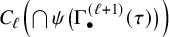 . We choose some arbitrary
$\alpha \in C_{\ell +1} \left ( \bigcap \psi \big ( \Gamma ^{(\ell +1)}_{\bullet }(\tau ) \big ) \right )$
 such that
$\partial \alpha = f_{\bullet }^{(\ell +1)}(\partial \tau )$
 , and set

Therefore
$f^{(\ell +1)}_{\bullet }$
 is indeed a chain map from
$C_{\bullet }(Y_{\ell +1})$
 to
$C_{\bullet }\left (X\right )$
 . Note that by (4.7), it follows that
$f_{\bullet }^{(\ell +1)}$
 is nontrivial because
$f_{\bullet }^{(\ell )}$
 is nontrivial and
$\Phi $
 , being a subgrid, maps each vertex to a single vertex. Moreover, by construction
$f^{(\ell +1)}_{\bullet }$
 and
$\Gamma ^{(\ell +1)}$
 satisfy
$(P_{\ell +1})$
 . This concludes the proof of the induction step and of Lemma 4.1.
5 Homological minors in grid complexes
Let K be a simplicial complex on n vertices. The main goal in this section is to give a canonical construction of a generic chain map

for any
$m>\mu (K)$
 . Here, generic means that disjoint faces of K map to chains that avoid common alignments along axis-parallel hyperplanes. The precise statement (Lemma 5.1) is given in Section 5.1.
The construction of
$g_{\bullet }$
 is based on an adaptation of stair convexity to grid complexes. In Sections 5.2–5.4, we formally define stair convex chains and verify their compatibility with the boundary operator.
5.1 Generic chain maps into grid complexes
Consider chains
$\alpha \in C_k(G[n]^m)$
 and
$\beta \in C_\ell (G[n]^m)$
 . We say that the pair
$\{\alpha , \beta \}$
 is degenerate if there exist a k-cell
$\alpha _k \in \operatorname {\mathrm {supp}}(\alpha )$
 and an
$\ell $
 -cell
$\beta _\ell \in \operatorname {\mathrm {supp}}(\beta )$
 such that
$\alpha _k$
 and
$\beta _\ell $
 are contained in a common axis-parallel hyperplane
$\Pi _j(a) = \{(x_1, \dots , x_m)\in \mathbb {R}^m : x_j = a\}$
 . If the supports of
$\alpha $
 and
$\beta $
 contain no such pair of cells, then we say that the pair
$\{\alpha , \beta \}$
 is generic.
We extend the notion of genericity to chain maps as follows. Let K be a simplicial complex and consider a nontrivial chain map

We say that
$g_{\bullet }$
 is generic if every pair of disjoint simplices of K maps to a generic pair of chains of
$C_{\bullet }(G[n]^m)$
 . In other words,
$g_{\bullet }$
 is generic if

Roughly speaking, the following “Picasso Lemma” asserts that any simplicial complex can be realized within a (sufficiently large) grid complex via a generic chain map. (See Figure 6.)
Lemma 5.1. Let K be a simplicial complex on n vertices. For any
$m> \mu (K)$
 there exists a generic, nontrivial chain map
$g_{\bullet } \colon C_{\bullet }(K) \to C_{\bullet }(G[n]^m)$
 .
The graph
$K_5$
 (considered as a 1-dimensional simplicial complex) realized as a subcomplex of the grid complex
$G[5]^3$
 via the generic chain map given in Lemma 5.1.

Figure 6 Long description
The diagram is set within a 3D coordinate system defined by three axes with arrows.
* At the base is a 2D horizontal grid plane composed of a 5 by 5 square mesh.
* Suspended above this grid is a complex structure of blue lines and black nodes.
* Vertical dotted lines connect specific points on the horizontal grid to corresponding open blue circles in the elevated structure, indicating projection or mapping.
* The elevated structure consists of four parallel vertical paths that are interconnected by horizontal and diagonal blue segments.
* Most nodes are solid black dots, while the terminal points at the bottom of each vertical segment are represented by open blue circles.
* The structure forms a stepped, ladder-like appearance that rises as it moves from the foreground left toward the background right.
* The edges are strictly linear, forming a subcomplex that follows the paths of a larger implicit 3D grid.
Our proof of this lemma is based on stair convexity, which we introduce in Section 5.2. Sections 5.3 and 5.4 will establish auxiliary results and properties related to stair convexity, concluding with the proof of Lemma 5.1. First, we establish the following immediate consequence:
Corollary 5.2. Fix a d-dimensional simplicial complex K on n vertices and a simplicial complex X such that
$K\not \prec _H X$
 . Let Y denote the d-skeleton of
$G[n]^m$
 , where
$m> \mu (K)$
 . For every nontrivial chain map
$f_{\bullet } \colon C_{\bullet }(Y) \to C_{\bullet }(X)$
 there exist disjoint cells
$\sigma $
 and
$\tau $
 in Y satisfying:
-
(i) $\sigma $
and
$\tau $
are not contained in any common axis-parallel hyperplane. -
(ii) The supports of $f_{\bullet }(\sigma )$
and
$f_{\bullet }(\tau )$
are overlapping.


Proof. Fix a nontrivial chain map
$f_{\bullet } \colon C_{\bullet }(Y) \to C_{\bullet }(X)$
 . By Lemma 5.1, there exists a generic nontrivial chain map

Since K is d-dimensional, the image of
$g_{\bullet }$
 is contained in the d-skeleton of
$G[n]^m$
 (which is Y). Thus, the composition
$h_{\bullet } = f_{\bullet } \circ g_{\bullet }$
 is a well-defined, nontrivial chain map:

By the hypothesis
$K\not \prec _H X$
 , there exist disjoint simplices
$\sigma '$
 and
$\tau '$
 in K such that the supports of
$h_{\bullet }(\sigma ')$
 and
$h_{\bullet }(\tau ')$
 overlap. Because
$h_{\bullet }$
 factors through
$C_{\bullet }(Y)$
 , there must exist cells
$\sigma \in \operatorname {\mathrm {supp}}(g_{\bullet }(\sigma '))$
 and
$\tau \in \operatorname {\mathrm {supp}}(g_{\bullet }(\tau '))$
 such that the supports of
$f_{\bullet }(\sigma )$
 and
$f_{\bullet }(\tau )$
 overlap.
Since
$g_{\bullet }$
 is generic and
$\sigma '$
 and
$\tau '$
 are disjoint, the pair of chains
$\{g_{\bullet }(\sigma '), g_{\bullet }(\tau ')\}$
 is generic. By definition, this means that the cells
$\sigma $
 and
$\tau $
 are not contained in a common axis-parallel hyperplane.
Finally, since
$g_{\bullet }$
 preserves dimension, we have:

By Observation 3.1, if
$\sigma $
 and
$\tau $
 were to intersect, they would have to be contained in a common axis-parallel hyperplane. Since we have just established they are not,
$\sigma $
 and
$\tau $
 must be disjoint.
5.2 Stair convex chains
The stair convex hull was introduced by Bukh et al. [Reference Bukh, Matoušek and Nivasch10] as a tool for analyzing point configurations related to extremal problems in discrete geometry such as lower bounds on the size of weak
$\varepsilon $
 -nets. Here we define a particular class of chains in the grid complex
$G[n]^m$
 that resembles their recursive definition.
We fix some integer
$n \ge 2$
 and work implicitly in the grid complex
$G[n]^m$
 . For any integers
$m \ge k \ge 0$
 (with
$m\geq 1$
 ) and any sequence
$1\leq a_1 < \cdots < a_{k+1} \leq n$
 we define the stair convex k-chain
$\operatorname {\mathrm {sc}}^{m}_k(a_1,\ldots , a_{k+1}) \in C_k(G[n]^m)$
 . The definition is recursive:
$ \begin {array}{lrcl} \mathbf {(m>k=0)} & \operatorname {\mathrm {sc}}_0^m(a) & := & \overbrace {(a,\dots , a)}^{m\text {-fold}}\\ \mathbf {(m=k>0)} & \operatorname {\mathrm {sc}}_k^m(a_1, \dots , a_{m+1}) & := & [a_1,a_2] \times [a_2,a_3] \times \ldots \times [a_m,a_{m+1}]\\ \mathbf {(m>k>0)} & \operatorname {\mathrm {sc}}_k^m(a_1, \ldots , a_{k+1}) & := & \operatorname {\mathrm {sc}}^{m-1}_{k-1}(a_1, \ldots , a_k) \times [a_k,a_{k+1}]\\ &&& \quad +\ \operatorname {\mathrm {sc}}^{m-1}_k(a_1, \ldots , a_{k+1}) \times \{a_{k+1}\}\\ \end {array}$

Examples
At one end,
$\operatorname {\mathrm {sc}}_0^m(a)$
 is a vertex on the main diagonal of
$G[n]^m$
 . At the other end,
$\operatorname {\mathrm {sc}}_m^m(a_1, \dots , a_{m+1})$
 is an m-dimensional box. Let us examine some simple examples for intermediate values of k. For
$m=2$
 and
$k=1$
 we have

which is a rectilinear path from
$(a,a)$
 to
$(b,b)$
 with a bend at
$(a,b)$
 . Similarly,
$\operatorname {\mathrm {sc}}_1^3(a, b)$
 is a rectilinear path from
$(a,a,a)$
 to
$(b,b,b)$
 with bends at
$(a,a,b)$
 and
$(a,b,b)$
 :


For
$m=3$
 and
$k=2$
 , we get the following
$2$
 -chain:


5.3 Nonrecursive formulation
From the examples above, we glimpse a general pattern for “unwrapping” the recursive definition of
$\operatorname {\mathrm {sc}}^m_k$
 . We extend the definition of a stair convex chain to the case
$m=k=0$
 by setting, for any integer a and any chain
$\sigma $
 ,
$\operatorname {\mathrm {sc}}^0_0(a) \times \sigma = \sigma \times \operatorname {\mathrm {sc}}^0_0(a) = \sigma $
 . Note that
$\operatorname {\mathrm {sc}}^0_0(a)$
 acts as the identity with respect to
$\times $
 .
Lemma 5.3. For every
$m \ge k \ge 1$
 and any
$1 \le a_1 < a_2 < \ldots < a_{k+1} \le n$
 we have

Proof. We define
$s^m_0(a) := \operatorname {\mathrm {sc}}^m_0(a)$
 , and for
$m \geq k\geq 1$
 we denote by
$s^m_k(a_1, \dots , a_{k+1})$
 the right-hand term of the identity to prove. Note that
$s^m_k$
 immediately satisfies the first two relations that define
$\operatorname {\mathrm {sc}}^m_k$
 :

It therefore suffices to prove that
$s^m_k$
 also satisfies the third relation:

For
$m \ge k \ge 1$
 let us define

and note that these sets of vectors are pairwise disjoint. For
$(t_1, \ldots , t_{k+1}) \in I(m,k)$
 , let us define

In this notation, we have

Note that for
$(t_1, t_2, \ldots , t_{k+1}) \in I(m,k)$
 , we have

The desired identity now follows by splitting
$I(m,k)$
 into

and observing that
$(t_1, t_2, \ldots , t_{k+1}) \mapsto (t_1, t_2, \ldots , t_{k+1}-1)$
 defines a bijection between
$I_>(m,k)$
 and
$I(m-1,k)$
 , and that
$(t_1, t_2, \ldots , t_{k+1}) \mapsto (t_1, t_2, \ldots , t_{k})$
 defines a bijection between
$I_0(m,k)$
 and
$I(m-1,k-1)$
 .
Corollary 5.4. Let
$k < m$
 . An axis-parallel hyperplane
$\Pi _j(a) = \{(x_1, \dots , x_m)\in \mathbb {R}^m : x_j=a\}$
 contains a k-dimensional face of the support of
$\operatorname {\mathrm {sc}}^m_k(a_1, \dots , a_{k+1})$
 if and only if
$a \in \{a_1, \dots , a_{k+1}\}$
 .
Proof. By Lemma 5.3 we have

Note that the support of
$\operatorname {\mathrm {sc}}^m_k(a_1, \dots , a_{k+1})$
 is the union of the supports of the summands of the right-hand side. The support of a summand is contained in
$\Pi _j(a)$
 if and only if for some j we have
$t_j \neq 0$
 and
$a_{j} = a$
 .
5.4 Stair convex chains and the boundary operator
We start by proving that stair convex chains behave like k-dimensional simplices with respect to the boundary operator on grid complexes. Figure 7 illustrates this phenomenon in
$2$
 dimensions. To formalize this claim, let us define

that is,
$\widehat {\hspace {1ex}}$
 denotes the coordinate to be omitted. (Recall that all homology in this paper has coefficients in
$\mathbb {Z}_2$
 .)
Proposition 5.5. For integers
$m\geq k \geq 1$
 and any sequence
$a_1 < a_2 < \ldots < a_m$
 of elements from
$[n]$
 we have
$\displaystyle \partial \operatorname {\mathrm {sc}}^m_k(a_1, \dots , a_{k+1}) = {\sum _{i=1}^{k+1}}\: \operatorname {\mathrm {sc}}^m_{k-1}(a_1, \dots , \widehat {a_i}, \dots , a_{k+1})$
 .
On the left: An illustration of the 2-chain
$\operatorname {\mathrm {sc}}^2_2(a,b,c)$
 with highlighted boundary. On the right: An illustration of the boundary of
$\operatorname {\mathrm {sc}}^2_2(a,b,c)$
 decomposed into the sum of
$\operatorname {\mathrm {sc}}^2_1(a,b), \operatorname {\mathrm {sc}}^2_1(b,c)$
 , and
$\operatorname {\mathrm {sc}}^2_1(a,c)$
 , respectively. Note that both
$\{a\}\times [a,b]$
 and
$[b,c]\times \{c\}$
 cancel out since we work with
$\mathbb {Z}_2$
 coefficients.

Figure 7 Long description
The diagram consists of two panels showing geometric representations on x and y axes.
* Left Panel: A light blue square is positioned in the upper-left quadrant. Its horizontal span on the x-axis is from a to b, and its vertical span on the y-axis is from b to c. The square is labeled s c sub 2 super 2 (a, b, c) with a dark blue boundary.
* Right Panel: The same light blue square is shown, but its boundary is decomposed into three colored segments.
1. A green L-shaped path, labeled s c sub 1 super 2 (a, b), starts at point (a, a) and goes to (b, b).
2. A red L-shaped path, labeled s c sub 1 super 2 (b, c), starts at point (b, b) and goes to (c, c).
3. A dark blue L-shaped path, labeled s c sub 1 super 2 (a, c), forms the outer boundary of the square from the x-axis value a to the y-axis value c.
White circular nodes mark the coordinates (a, a), (b, b), and (c, c) along a diagonal trajectory. The overlapping vertical and horizontal segments between the colored paths indicate cancellation under Z sub 2 coefficients.
The proof is a somewhat lengthy, but straightforward, calculation that takes up most of this section. We set up an induction on m by using the recursive definition of
$\operatorname {\mathrm {sc}}^m_k$
 (for
$k<m$
 ) or by applying the product rule after singling out the factor
$[a_m,a_{m+1}]$
 (for
$k=m$
 ). One important trick is to handle the factors
$[a_{i-1},a_{i+1}]$
 arising from
$\operatorname {\mathrm {sc}}^m_{k-1}(a_1, \dots , \widehat {a_i}, \dots , a_{k+1})$
 using the identity
$[a_{i-1},a_{i+1}] = [a_{i-1},a_{i}] + [a_{i},a_{i+1}]$
 between
$1$
 -chains. Our first step is to establish a simpler identity.
Lemma 5.6. For any
$m \geq 1$
 and
$1 \le a_1 < a_2 < \ldots < a_{m+2} \leq n$
 we have

Proof. For
$m=1$
 , this is a reformulation of
$[a_1,a_3]= [a_1,a_2] + [a_2,a_3]$
 which holds by definition whenever
$a_1, a_2$
 , and
$a_3$
 are distinct. For
$m \ge 2$
 , we have

since
$[a_{m}, a_{m+2}]+[a_{m}, a_{m+1}]= [a_{m+1}, a_{m+2}]$
 (here we use that the
$a_i$
 are distinct). The statement therefore follows by induction on m.
Let us return to the proof of the claim that stair convex chains behave as simplices for the boundary operator on
$G[n]^m$
 .
Proof of Proposition 5.5. The case
$m=1$
 follows directly from the definition of the boundary operator.
Case
$\mathbf {m=k\geq 2}$

Here, we proceed by induction on m, and assume that the statement holds for
$m-1$
 :

From the definition of
$\partial $
 we get

We then use the induction hypothesis to rewrite
$\alpha $
 as

and use Lemma 5.6 to partially expand
$\beta $
 into

For
$i \le m-1$
 , we have
$\alpha _i + \beta _i = \operatorname {\mathrm {sc}}^{m}_{m-1}(a_1, \dots , \widehat {a_i}, \dots , a_{m+1})$
 by the recursive definition of
$\operatorname {\mathrm {sc}}^{m}_{m-1}$
 . For the same reason, for any
$a \in [n]$
 ,

Since the
$a_i$
 are pairwise distinct, we have
$[a_m,a_{m+1}] = [a_{m-1},a_m] + [a_{m-1},a_{m+1}]$
 . Using Identity (5.2) once with
$a=a_m$
 and once with
$a=a_{m+1}$
 , we obtain

Altogether,

as claimed.
General case
We now prove the general case by induction on m. So assume the statement holds for
$m-1$
 and consider
$1 \le k \le m$
 . We already handled the case
$k=m$
 , so let us consider the case
$k<m$
 , for which we can use the recursive definition of
$\operatorname {\mathrm {sc}}^m_k$
 :

We thus have

Using the induction hypothesis for
$\operatorname {\mathrm {sc}}^{m-1}_{k-1}$
 and
$\operatorname {\mathrm {sc}}^{m-1}_{k}$
 , we obtain

For
$i \le k-1$
 , we recognize the recursive definition of
$\operatorname {\mathrm {sc}}^{m}_{k-1}$
 in

Since the elements
$a_1, \ldots , a_{k+1}$
 are pairwise distinct,
$[a_k,a_{k+1}] = [a_{k-1},a_k] + [a_{k-1},a_{k+1}]$
 and we can split
$\alpha _k$
 and use the recursive definition of
$\operatorname {\mathrm {sc}}^{m}_{k-1}$
 on each part:

Altogether,

as claimed.
Finally, we are now in position to prove the “Picasso Lemma”.
Proof of Lemma 5.1
Label the vertices of K as
$v_1, v_2, \dots , v_n$
 . For every simplex
$\{v_{i_1}, \dots , v_{i_{k+1}}\} \in K$
 with
$1\leq i_1 < i_2 <\cdots < i_{k+1}\leq n$
 , we define:

We extend g linearly into a map
$g_{\bullet } \colon C_{\bullet }(K) \to C_{\bullet }(G[n]^m)$
 . Proposition 5.5 guarantees that
$g_{\bullet }$
 commutes with the boundary operator, making it a valid chain map. Furthermore, since every vertex
$v_a\in V(K)$
 is mapped to a single vertex
$\{a\}\times \cdots \times \{a\}\in G[n]^m$
 , the map is nontrivial.
To show that
$g_{\bullet }$
 is generic, let
$\sigma $
 and
$\tau $
 be a pair of disjoint simplices in K, and consider arbitrary cells
$\sigma ' \in \operatorname {\mathrm {supp}}(g_{\bullet }(\sigma ))$
 and
$\tau ' \in \operatorname {\mathrm {supp}}(g_{\bullet }(\tau ))$
 . Since
$m> \mu (K)$
 (implies
$\dim \sigma + \dim \tau < m$
 ), it follows that
$\dim \sigma ' + \dim \tau ' < m$
 . By Observation 3.1, there is at least one coordinate,
$x_i$
 , that is constant for both cells. However, they cannot share the same constant value in this coordinate (i.e.,
$x_i = a$
 is impossible for both), because Corollary 5.4 would imply that both
$\sigma $
 and
$\tau $
 contain the vertex
$v_a$
 , contradicting their disjointness. Thus, the pair
$\{g_{\bullet }(\sigma ), g_{\bullet }(\tau )\}$
 is generic.
Remark. The reader may note (as can be formalized using [Reference Bukh, Matoušek and Nivasch10, Lemma 1.4]) that mapping simplices to stair convex chains generated by points on the main diagonal of the grid complex closely resembles the canonical geometric realization of a simplicial complex via the moment curve.
6 Wrapping up
We now have all the ingredients to prove Theorems 2.1 and 1.5. We start with our weak colorful Helly theorem, which we restate here for convenience.
Theorem 2.1 (Weak colorful Helly theorem)
For any finite simplicial complex K and integers
$b\geq 1$
 and
$m> \mu (K)$
 , there exists an integer
$t = t(b,K,m)$
 with the following property: If
$\mathcal {F} = \mathcal {F}_1 \sqcup \cdots \sqcup \mathcal {F}_m$
 is an m-colored
$(K,b)$
 -free cover where each color class has size t and every colorful subfamily has nonempty intersection, then
$\mathcal {F}$
 contains some
$2m-\mu (K)$
 members with nonempty intersection.
Proof. Let n be the number of vertices in K and let d be the dimension of K. We will show that the theorem holds with
$t \leq t(b,d,m,n)$
 as given by Lemma 4.1.
To this end, let
$\mathcal {F}$
 be an m-colored
$(K,b)$
 -free cover where each color class has size
$t = t(b,d,m,n)$
 and every colorful subfamily has nonempty intersection. Then
$\mathcal {F}$
 satisfies the conditions of Lemma 4.1, and so there exists a nontrivial chain map

that is constrained by
$\mathcal {F}$
 , where Y denotes the d-skeleton of
$G[n]^m$
 . This means there is a subgrid
$\Gamma : V(G[n]^m) \to V(\text{Grd}_{\mathcal {F}})$
 such that
$\operatorname {\mathrm {supp}} f_{\bullet }(\sigma )\subset \bigcap \psi \left (\Gamma _{{\bullet }}(\sigma )\right )$
 for every
$\sigma \in Y$
 .
Since
$m> \mu (K)$
 the chain map
$f_{\bullet }$
 also satisfies the conditions of Corollary 5.2 (where Y still denotes the d-skeleton of
$G[n]^m$
 ). Therefore we can find two disjoint cells
$\sigma $
 and
$\tau $
 in Y that satisfy:
-
(i) $\sigma $
and
$\tau $
are not contained in a common axis-parallel hyperplane. -
(ii) The supports of $f_{\bullet }(\sigma )$
and
$f_{\bullet }(\tau )$
overlap.


Since
$f_{\bullet }$
 is constrained by
$\mathcal {F}$
 , condition (ii) implies that there is a point contained in every member of the union
$\psi \left (\Gamma _{\bullet }(\sigma )\right ) \cup \psi \left ({\Gamma _{\bullet }(\tau )}\right )$
 . From (i) and Claim 3.2 (iii) it follows that the colorful families
$\psi \left (\Gamma _{\bullet }(\sigma )\right )$
 and
$\psi \left ({\Gamma _{\bullet }(\tau )}\right )$
 are disjoint. Finally, we compute the size of this union:

(Note that the last inequality uses that
$\sigma $
 and
$\tau $
 are disjoint.)
Last, we spell out the use of supersaturation outlined in Section 2.2 to prove the stepping-up theorem using our weak colorful Helly theorem.
Let us recall some (standard) terminology on hypergraphs. An m-uniform hypergraph is a pair
$H=(V,E)$
 where
$V=V(H)$
 is a finite set of vertices and
$E=E(H)\subset \binom {V}{m}$
 is the edge set. An m-uniform hypergraph is m-partite if the vertex set can be partitioned into disjoint sets (parts)
$V(H) = V_1 \cup \cdots \cup V_m$
 such that every edge contains exactly one vertex from each
$V_i$
 . Given integers
$m\geq 2$
 and
$t \geq 1$
 , we let
$K^m(t)$
 denote the complete m-partite m-uniform hypergraph with parts
$V_1, \dots , V_m$
 where
$|V_i|=t$
 . That is, the edge set of
$K^m(t)$
 consists of all m-tuples of
$V_1 \cup \cdots \cup V_m$
 that contain exactly one element from each
$V_i$
 .
A hypergraph H contains a hypergraph
$H'$
 if there is an injection
$f: V(H') \to V(H)$
 such that for every
$e' \in E(H')$
 ,
$f(e') \in E(H)$
 . (In particular, we do not require
$H'$
 to be an induced sub-hypergraph of H.) We use the following supersaturation theorem of Erdős and Simonovits:
Theorem (Erdős-Simonovits [Reference Erdős and Simonovits20, Corollary 2])
For any positive integers m and t and any
$\varepsilon>0$
 there exists
$\rho = \rho (\varepsilon , m, t)>0$
 such that any m-uniform hypergraph
$H = (V,E)$
 with
$|E|\geq \varepsilon \binom {|V|}{m}$
 contains at least
$\rho |V|^{mt}$
 copies of
$K^m(t)$
 .
For convenience, we restate our final theorem.
Theorem 1.5 (Stepping-up theorem)
Fix a simplicial complex K, a value
$\delta \in (0,1]$
 , and integers
$b\geq 1$
 and
$m> \mu (K)$
 . If
$\mathcal {F}$
 is a sufficiently large
$(K,b)$
 -free cover such that
$\pi _m(\mathcal {F})\geq \delta \binom { | \mathcal {F} | }{m}$
 , then
$\pi _{m+1}(\mathcal {F})\geq \gamma \binom { | \mathcal {F} |}{m+1}$
 , where
$\gamma> 0$
 is a constant that depends only on
$\delta $
 , b, m, and K.
Proof. Fix a simplicial complex K and integers
$b\geq 1$
 and
$m> \mu (K)$
 . Let
$t=t(b,K,m)$
 be the constant from Theorem 2.1. Consider some
$(K,b)$
 -free cover
$\mathcal {F}$
 .
For a subfamily
$\mathcal {F}' \subseteq \mathcal {F}$
 , let
$H[\mathcal {F}']$
 be the m-uniform hypergraph whose vertices are the members of
$\mathcal {F}'$
 and whose edges are the m-tuples of
$\mathcal {F}'$
 with nonempty intersection. By assumption, our hypergraph
$H[\mathcal {F}]$
 contains at least
$\delta \binom {|\mathcal {F}|}{m}$
 edges. By the Erdős–Simonovits theorem, for some constant
$\rho>0$
 depending only on m, t, and
$\delta $
 , there are at least
$\rho \binom {|\mathcal {F}|}{mt}$
 distinct
$mt$
 -element subfamilies
$\mathcal {F}'$
 of
$\mathcal {F}$
 such that
$H[\mathcal {F}']$
 contains a copy of
$K^m(t)$
 .
Our choice of t ensures that Theorem 2.1 applies to every such subfamily
$\mathcal {F}'$
 , and therefore each
$\mathcal {F}'$
 contributes some
$2m-\mu (K)\ge m+1$
 members with nonempty intersection. Each
$(m+1)$
 -element subset of
$\mathcal {F}$
 with nonempty intersection is contained in
$\binom {|\mathcal {F}|-(m+1)}{mt-(m+1)}$
 distinct
$(mt)$
 -tuples
$\mathcal {F}'$
 . There are therefore at least

$(m+1)$
 -tuples of
$\mathcal {F}$
 with nonempty intersection. In other words,
$\pi _{m+1}(\mathcal {F})$
 is at least
$\delta ' := \rho /\binom {mt}{m+1}$
 , where
$\rho $
 depends only on m, t, and
$\delta $
 , that is, on m, b, K, and
$\delta $
 . That concludes the proof.
7 Discussion and outlook
In conclusion, let us comment on some related problems and future work.
Topological generalizations of Helly’s theorem
Relaxing the convexity assumption in Helly’s theorem is a classical question that goes back to the topological Helly theorem [Reference Helly24, Reference Debrunner14], which asserts that Helly’s theorem holds for finite good covers. The fractional Helly theorem and the
$(p,q)$
 -theorem also hold for finite good covers [Reference Alon, Kalai, Matoušek and Meshulam3].
These results were, in turn, extended to families in which intersections have a bounded number of connected components, all contractible [Reference Matoušek35, Reference De Verdière, Ginot and Goaoc16, Reference Kalai and Meshulam32], then to families in which intersections have bounded Betti numbers [Reference Goaoc, Paták, Patáková, Tancer and Wagner21, Reference Patáková39]. At their core, these extensions rely either on variants of the Nerve Theorem and the Vietoris-Begle Theorem [Reference De Verdière, Ginot and Goaoc16, Reference Kalai and Meshulam32] or on variants of the Van Kampen-Flores Theorem [Reference Matoušek35, Reference Goaoc, Paták, Patáková, Tancer and Wagner21, Reference Patáková39] (see also the survey [Reference Paták and Patáková38]). The latter works readily generalize to the setting of complexes with a forbidden homological minor, with the Van Kampen-Flores Theorem being one specific forbidden homological minor for
$\mathbb {R}^d$
 .
In particular, our
$(p,q)$
 -theorem 1.4 implies that for every
$p\geq q \geq d+1$
 and
$b\geq 1$
 , the assertion of the
$(p,q)$
 -theorem holds for any finite family of sets in
$\mathbb {R}^d$
 such that the intersection of every subfamily has ith reduced Betti number less than b for
$0 \le i < \lceil d/2\rceil $
 . Note that the constant number of points given by the
$(p,q)$
 -theorem in this case depends not only on p, q, and d, but also on b.
A natural question is whether the
$(p,q)$
 -theorem generalizes to families of sets in manifolds. For surfaces, this is the case as we can improve [Reference Patáková39, Theorem 2.6]. Specifically, our
$(p,q)$
 -theorem 1.4 implies that for every
$p\geq q \geq 3$
 and
$b\geq 1$
 , the assertion of the
$(p,q)$
 -theorem holds for any finite family of sets on a compact,
$2$
 -dimensional real manifold, such that the intersection of every subfamily has at most b path-connected components. (Here the constant number of points depends not only on p, q, d, and b, but also on the surface considered.) We conjecture that it extends to higher-dimensional manifolds as well.
Conjecture 7.1. For every d-dimensional manifold M, there exists a simplicial complex
$K_M$
 with
$\mu (K_M) = d$
 such that for any triangulation X of M, we have
$K_M\not \prec _H X$
 .
We remark that some version of Conjecture 7.1 was very recently settled in the affirmative by Avvakumov, Bin and Goaoc [Reference Avvakumov, Bin and Goaoc6].
Upper-bound theorems
In fractional Helly theorems, the main parameter one usually tries to optimize is the fractional Helly number. In that respect, our Theorem 1.6 is very satisfying: the bound is independent of b and is sharp for at least some forbidden homological minors. The next parameter that one may try to improve is the dependency between the size of the large intersecting family (the
$\beta $
 ) and the proportion of intersecting few-tuples (the
$\alpha $
 ).
In the convex case, the original fractional Helly theorem of Katchalski and Liu [Reference Katchalski and Liu34] gave
$\beta \ge \frac {\alpha }{d+1}$
 . They also showed that one may assume that
$\beta (\alpha ) \to 1$
 when
$\alpha \to 1$
 . Their proof uses the observation, which they dubbed the stepping-up lemma, that for any
$0 < \alpha \le 1$
 , any
$d < k < \ell $
 , and any finite family
$\mathcal {F}$
 of convex sets in
$\mathbb {R}^d$
 ,

In particular, if
$\alpha> 1-1/\binom {\ell -1}{k-1}$
 , then a positive proportion of the
$\ell $
 -element subfamilies of
$\mathcal {F}$
 have nonempty intersection. Our stepping-up theorem 1.5 asserts that this propagation of positive densities holds more generally for
$(K,b)$
 -free covers.
For convex sets, the optimal dependency of
$\beta $
 on
$\alpha $
 was established by Kalai as
$\beta \ge 1-(1-\alpha )^{\frac 1{d+1}}$
 . Kalai’s proof is based on the upper bound theorem that he [Reference Kalai28] and Eckhoff [Reference Eckhoff18] established independently. The upper bound theorem asserts that for any family
$\mathcal {F}$
 of n convex sets in
$\mathbb {R}^d$
 , for any k such that
$d < k \le d+r$
 ,

This was recently extended to more general set systems in
$\mathbb {R}^2$
 and in surfaces [Reference Kalai and Patáková33, Theorem 2.2 and 2.3]. Our fractional Helly theorem shows some form of an upper bound theorem for
$(K,b)$
 -free covers. We did not try to extract it as we believe it is quantitatively rather weak.
Question 7.2. What is the best possible upper bound theorem for
$(K,b)$
 -free covers?
Collapsibility and Lerayness
The known proofs of the upper bound theorem (7.2) are typically more general than the geometric setting, and deal with certain properties of nerves of families of convex sets. The more elementary proofs apply to d-collapsible complexes [Reference Eckhoff18, Reference Kalai28, Reference Alon and Kalai2], that is, complexes that can be reduced by discrete homotopy moves (called collapses) to a d-dimensional complex [Reference Wegner42, Lemma 1]. The more general proof, also due to Kalai (a presentation can be found in Hell’s PhD thesis [Reference Hell23,
$\S 5.2$
 ]), applies to d-Leray complexes, that is, complexes in which all induced subcomplexes have vanishing homology in dimension d and above. Theorem 1.5 reveals that nerves of
$(K,b)$
 -free covers enjoy some of the consequences of bounded Lerayness. More generally, we conjecture:
Conjecture 7.3. For any simplicial complex K and positive integer b, the nerve of any
$(K,b)$
 -free cover is L-Leray, where L depends only on K and b.
We note that L must be at least
$b(\mu (K)+2)-1$
 [Reference Goaoc, Paták, Patáková, Tancer and Wagner21, Example 2]. A first step in this direction was done by Holmsen et al. [Reference Holmsen, Kim and Lee26], who considered the special case when
$\mathcal {F} = \{G_i\}$
 is a family of connected subgraphs of a graph G such that any nonempty intersection of members of
$\mathcal {F}$
 is also connected. They conjectured that for any
$r\geq 1$
 , if
$K_{r+2}$
 is not a minor of G, then the nerve of
$\mathcal {F}$
 is r-Leray, and verified this for
$r\leq 3$
 . It should be noted that in [Reference Holmsen, Kim and Lee26] they deal with graph minors and not homological minors.
Homological VC dimension
Deeper connections between discrete geometry and topological combinatorics were suggested by Kalai and Meshulam in a program to develop a theory of homological VC dimension. For a positive integer h and a family
$\mathcal {F}$
 of sets in
$\mathbb {R}^d$
 , let us call the function

the (hth) homological shatter function of
$\mathcal {F}$
 . The combination of two conjectures of Kalai and Meshulam suggests that families of open sets in
$\mathbb {R}^d$
 with polynomial homological shatter function should satisfy a fractional Helly theorem:
Conjecture 7.4 (Following [Reference Kalai29, Conjectures 6 and 7])
For any integer
$0 \le m \le d$
 and any constant
$C>0$
 , there exists a function
$\beta :(0,1) \to (0,1)$
 such that the following holds. For any
$\alpha>0$
 and any sufficiently large finite family
$\mathcal {F}$
 of open sets in
$\mathbb {R}^d$
 with
$\phi ^{(d)}_{\mathcal {F}}(k) \le Ck^m$
 , if
$\pi _{d+1}(\mathcal {F}) \ge \alpha \binom {|\mathcal {F}|}{d+1}$
 , then some
$\beta (\alpha )|\mathcal {F}|$
 members of
$\mathcal {F}$
 have a point in common.
A combination of Conjectures 6 and 7 from [Reference Kalai29] also appeared in [Reference Kalai30, Conjecture 17]. Here we took upon ourselves to dissociate the dimension d of the space and the degree m of the polynomial bounding the homological shatter function. We give in to the temptation to generalize this conjecture to K-free covers, that is to finite families
$\mathcal {F}$
 of (not necessarily induced) subcomplexes of a simplicial complex X such that
$K \not \prec _H X$
 . We propose the following more general conjecture:
Conjecture 7.5. For any simplicial complex K, integer
$t \ge 0$
 , and constant
$C>0$
 , there exists a function
$\beta :(0,1) \to (0,1)$
 such that the following holds. For any
$\alpha>0$
 and any sufficiently large K-free cover
$\mathcal {F}$
 with
$\phi ^{(\dim K)}_{\mathcal {F}}(k) \le Ck^t$
 , if
$\pi _{\mu (K)+1}(\mathcal {F}) \ge \alpha \binom {|\mathcal {F}|}{\mu (K)+1}$
 , then some
$\beta (\alpha )|\mathcal {F}|$
 members of
$\mathcal {F}$
 have a point in common.
In other words, we conjecture a fractional Helly theorem for K-free covers whose
$(\dim K)$
 th homological shatter function is bounded by a polynomial of degree t. Our Theorem 1.6, by taking
$b> C$
 , resolves the
$t=0$
 case of this conjecture.
The technique we developed to prove our stepping-up theorem 1.5 actually shows that if Conjecture 7.5 holds with some fractional Helly number h, then it holds with the fractional Helly number
$\mu (K)+1$
 as claimed. Indeed our construction of a constrained chain map does not use the full power of the assumption that the colored family
$\mathcal {F}$
 is
$(K,b)$
 -free. Specifically, to obtain the conclusion of Lemma 4.1, it suffices that the m-colored family
$\mathcal {F}$
 of subcomplexes of X satisfies the following “sliding window” assumption:
The jth reduced Betti number
$\tilde {\beta }_j(\bigcap _{S \in \mathcal {G}}S)$
 is strictly less than b for all
$0\leq j < d$
 and all colorful subfamilies
$\mathcal {G} \subseteq \mathcal {F}$
 with
$|\mathcal {G}|=m-j-1$
 .
This change does not affect the bound on
$t(b,d,m,n)$
 . This in turn leads to a stepping-up theorem with weaker assumptions:
Theorem 7.6. Fix a simplicial complex K, a value
$\delta \in (0,1]$
 , and integers
$b\geq 1$
 and
$m> \mu (K)$
 . If
$\mathcal {F}$
 is a K-free cover such that
-
(i) $\tilde {\beta }_j(\bigcap _{S\in \mathcal {G}} S) < b$
, for all
$0\leq j < \dim K$
and
$\mathcal {G} \subseteq \mathcal {F}$
with
$|\mathcal {G}|=m-j-1$
, and -
(ii) $\pi _m(\mathcal {F}) \geq \delta \binom {|\mathcal {F}|}{m}$
,


then
$\pi _{m+1}(\mathcal {F}) \geq \gamma \binom {|\mathcal {F}|}{m+1}$
 , where
$\gamma $
 is a constant that depends only on
$\delta $
 , b, m, and K.
Now, suppose the fractional Helly number of
$\mathcal {F}$
 is bounded by some number h. Starting with the assumption that a positive fraction of the
$(\mu (K)+1)$
 -tuples of
$\mathcal {F}$
 are intersecting, we can apply Theorem 7.6 with
$m = \mu (K)+1, \ldots , h$
 (and in each case
$b = Cm^t$
 ) to eventually get that a positive fraction of the h-tuples of
$\mathcal {F}$
 are intersecting, and then apply that fractional Helly theorem.
Acknowledgments
The authors are grateful to an anonymous referee for valuable comments and suggestions that improved the manuscript.
Competing interests
The authors have no competing interest to declare.
Funding statement
X.G. and A.F.H. were supported by the INRIA associate teams FIP and DIPPS. A.F.H. was also supported by the National Research Foundation of Korea (NRF) grants funded by the Ministry of Science and ICT (NRF-2020R1F1A1A01048490) and the Institute for Basic Science (IBS-R029-C1). Z.P. was supported by the Charles University project PRIMUS/21/SCI/014 and also by the GAČR grant no. 25-16847S.


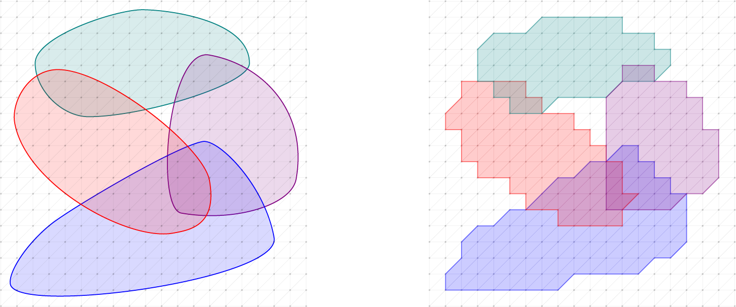


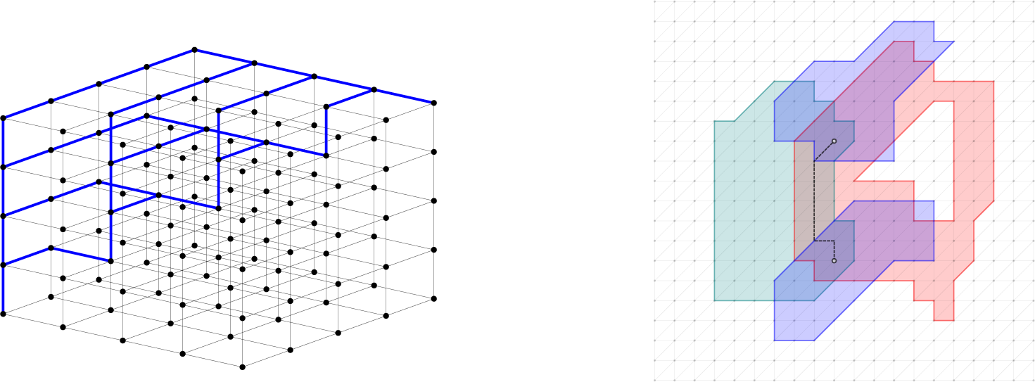


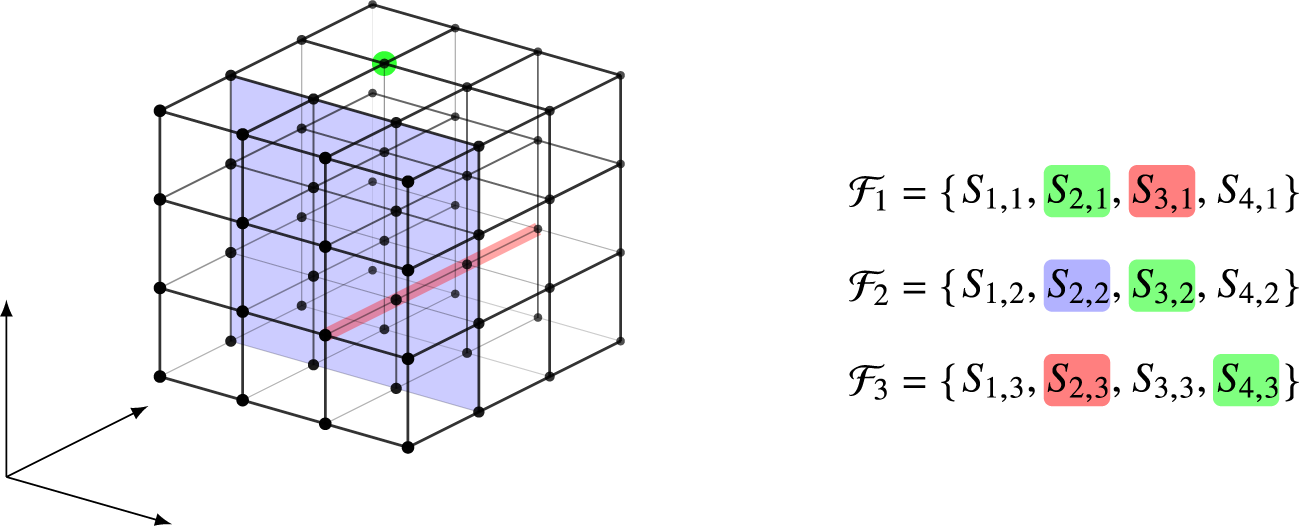


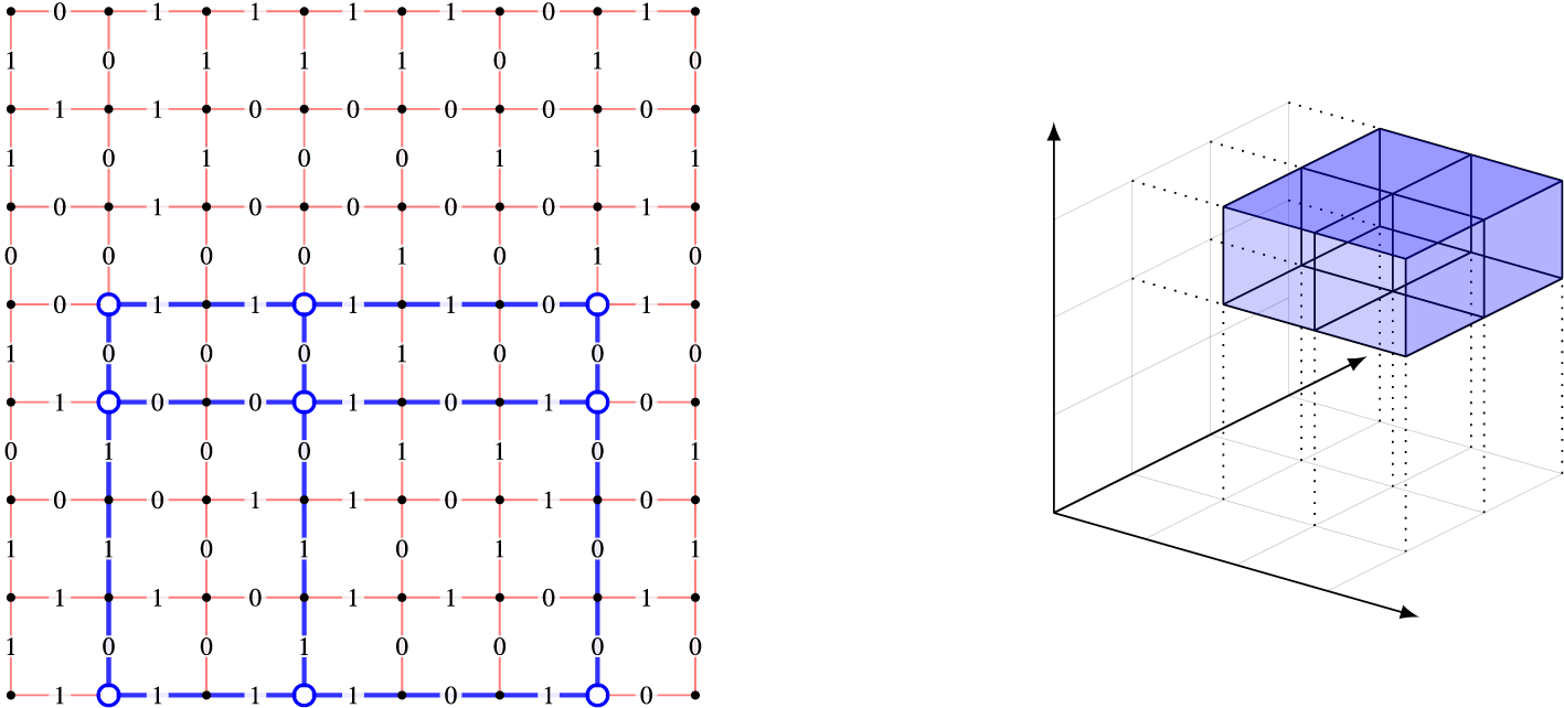


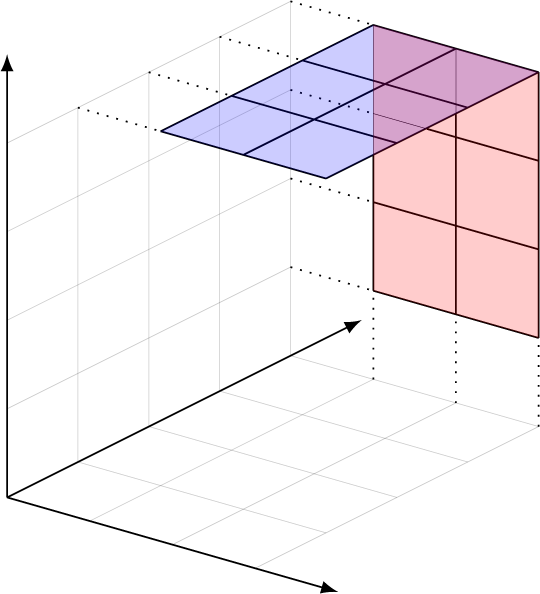


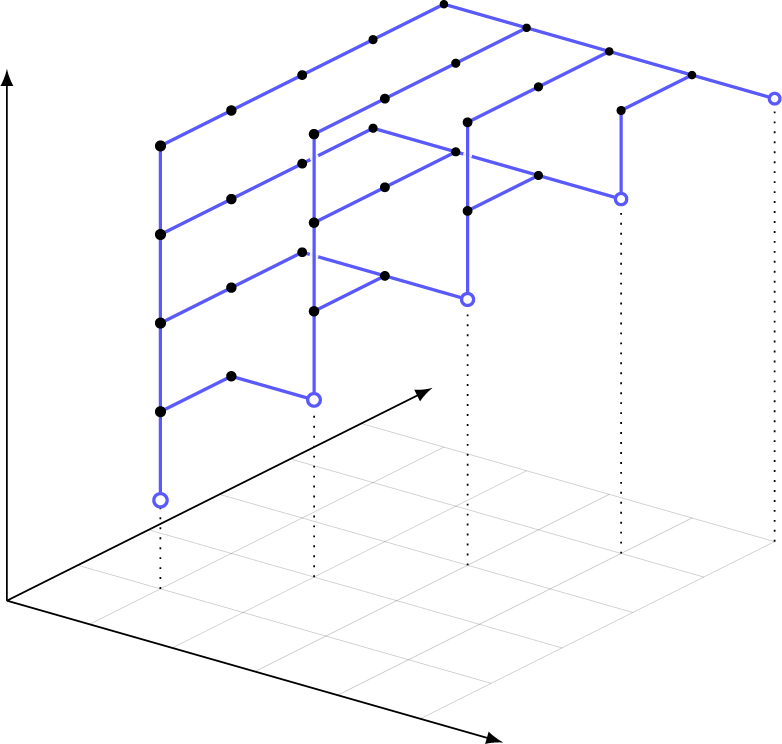


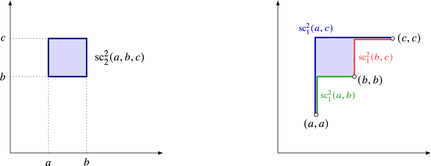


 Open access

