The trial-heat poll and economy forecasting model is a simple model based on a simple principle.1
The basic model was first presented by Campbell and Wink (1990), corroborating an earlier finding by Lewis-Beck and Rice (Lewis-Beck 1985). The current version differs in two ways from the original. First, because the BEA changed their featured broad-based economic measure from GNP to GDP, and consequently the timing of the release of these measures, the model switched from using the second-quarter growth rate in GNP to the second-quarter growth rate in GDP. Second, in examining open-seat presidential elections after the 2000 election, the model revised the economic growth measure to award half credit or blame to the in-party candidate (Campbell 2001a; 2001b). Also, GDP growth is now included in the equation as an annualized measured.
The model uses just two predictor variables to forecast the in-party presidential candidate's share of the national two-party popular vote. The first is the in-party presidential candidate's share of support between the major party candidates in the Gallup Poll's trial-heat (or preference) poll question around Labor Day. The second predictor is the Bureau of Economic Analysis' (BEA) measure of real growth in the Gross Domestic Product (GDP) in the second quarter of the election year (April through June). The GDP measurement is the “preliminary” measure released by the BEA at the end of August, the latest available in time to be used in the forecast. An in-party presidential candidate who is the incumbent is accorded full responsibility for the economy in the equation and a successor or non-incumbent in-party candidate is accorded half the credit or blame for the growth or decline in the economy. This partial credit or blame for successor candidates refl ects both past experience in forecasting (Campbell
2000) and independent findings regarding the effects of retrospective evaluations of the economy on voting behavior (Nadeau and Lewis-Beck
2001). The regression estimated forecasts based on these two predictors, estimated over the 14 presidential elections from 1948 to 2000, is a mix of about two-thirds trial-heat poll and one-third economic growth. In essence, with the preference poll at the center of the prediction, the forecast may be interpreted as an
adjusted preference poll.
The principle behind the forecast model is that preference poll data may be more telling about elections if polls are read in their historical and contemporary contexts rather than accepted at face value. By the historical context of the poll, I mean what could be generally expected as a vote for a candidate (based on past experience) who has a certain percentage of support in the polls at a particular time in the campaign. By the contemporary context of the poll, I mean what could be generally expected as a vote for a candidate with a certain level of poll support when conditions in the current campaign (not already incorporated into the level of poll support) are more or less inclined for or against the in-party. The best indicator available of this contemporary context that is not already refl ected in candidate support tapped by the polls is the real growth rate in the economy (as measured by the GDP) during the second quarter of the election year. The use of the economic growth measure is not based on the premise that voters are largely economically driven, but that a strong economy enhances the public's receptivity to the in-party candidate and that a weak economy diminishes the public's receptivity to the in-party's message.2
The standardized coefficients for the forecast equation (Equation 1 in Table 1) indicate that second-quarter GDP growth is the junior partner in the forecast.
The use of only the second quarter economic growth rate also does not imply that voters care only about the economy in the election year. Earlier economic growth is already incorporated into the poll numbers and later growth (third quarter of the election year) appears to be too late to affect the vote, and in any event is too late to be of possible use in making a forecast. The theory of campaign effects providing the basis for this forecasting model is available in
The American Campaign (2000).
The Accuracy of Preference Poll-Based Forecasts
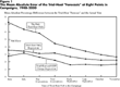
Figure 1 displays the greater forecast accuracy achieved by reading the preference polls in their contexts. The figure tracks the mean absolute errors in elections from 1948 to 2000: (1) of reading trial-heat polls as literal forecasts of the vote, (2) of producing a forecast based on the historical relationship of the polls to the vote as estimated through a bivariate regression, and (3) of producing a forecast based on the relationship of both the polls and the election-year economy on the vote. The errors for the bivariate and multivariate regressions are out-of-sample errors.3
Out-of-sample expected votes are examined to avoid the circularity of a model estimated based partially on data from an election being used to “predict” the vote in that election. In terms of actual forecasts, the model was first used in 1992 and was .6 of a percentage point off. The forecast error was 3.7 percentage points in 1996 and 2.5 percentage points in 2000.
As is clear from the figure, at each of the eight points during the election year, forecasts drawn from the combination of the trial-heat polls and the economy are generally more accurate than those drawn from the trial-heat alone regression and the trial-heat alone regression forecasts are more accurate than accepting the preference poll results at face value. The polls taken as literal forecasts before the party conventions are actually less accurate in general than the null hypotheses (either guessing a 50-50 split or the mean in-party vote of 52.5%). The mean absolute error of these null forecasts are both 4.8 percentage points and the raw polls do not achieve even this degree of accuracy until after the conventions.
4 The weakness of the early preference polls are also refl ected in how frequently the trailing candidate went on to win the popular vote plurality. From 1948 to 2000, the candidate trailing in the June preference poll won the popular vote nearly half the time (in six of the 14 elections).
On the other hand, even at their worst (in June), the regression models are only about 3.6 points off on average. Even at this early point in the campaign, this represents a substantial improvement over the null forecasts.
The Mean Absolute Error of the Trial-Heat “Forecasts” at Eight Points in Campaigns, 1948–2000
As is also clear from the figure, whether using the unadjusted polls, the trial-heat bivariate regression, or the trial-heat and economy regression, the accuracy of predictions generally improves the later the poll is taken in the campaign. The most important exception to this tendency is that the forecast accuracy of the trialheat and economy regression does not substantially improve after early September. The mean absolute error (out-of-sample) in the early September forecast, using both the poll and the economic growth rate, is only 1.6 percentage. The mean errors of the model in late September, mid-October, and at the beginning of November differ by less than a tenth of a percentage point from the mean early September error. For comparison, the mean absolute error of the preference poll two months later, just before the election in November, is a full percentage point higher. The mean absolute error of the early September poll accepted as a literal forecast is nearly two and a half times larger than the out-of-sample forecast produced by the regression of the poll and economic growth (3.9 compared to 1.6). As these comparisons make plain, the adjustment of the trial-heat poll by its historical relationship to the vote and the contemporary context refl ected in the economic growth in the second-quarter of the election year improves the forecasting accuracy of the poll enormously.
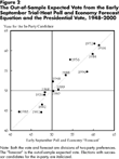
In comparing the errors across time, it is quite apparent that the optimal presidential vote forecast equation using preference polls is the early September poll and economy equation. Earlier forecasts are less accurate and later forecasts are not any more accurate. Figure 2 displays a plot of the out-of-sample expected vote from the early September preference poll and economy equation against the actual vote for the in-party candidate for the 14 elections from 1948 to 2000. The figure displays how close the out-of-sample “forecasts” have been to the actual vote. The elections gather quite closely to the diagonal where the vote would be exactly as expected. This was true in periods of strong partisanship (the 1950s and 1990s) and weakened partisanship (1970s). It was also true in elections conducted during times of war as well as when the nation was at peace. The figure also makes clear just how unusual it is for the in-party candidate to do poorly in elections. Of the 14 elections, the inparty candidate failed to receive a vote plurality in six—about what you would expect from the toss of a coin. However, three of these six losses were very close elections and the in-party candidate's vote never dipped below 44.6% of the two-party vote (Stevenson in 1952) in this set of elections. The poorest showing by an incumbent was 44.7% of the two-party vote (Carter in 1980).
The Out-of-Sample Expected Vote from the Early September Trial-Heat Poll and Economy Forecast Equation and the Presidential Vote, 1948–2000
Although the out-of-sample errors indicate that the early September forecast equation is quite accurate, this is not the sole basis for confidence in the equation. The fact that the equation is built around the preference polls (a measure of public opinion that explicitly recognizes the opposition candidate (unlike the approval measures)), is increasingly accurate until early September, is about as accurate as three later timings of the model (late September, October, and November), and has coefficients that vary in an expected way (with the poll becoming a stronger component and the economy becoming a weaker component of the forecast in later estimations) are also reasons to believe that the model is credible. The equation also finds support in an empirically supported theory of presidential campaign effects (Campbell 2000).
Equation 1 in Table 1 presents the OLS estimates of the early September trial-heat poll and second quarter GDP growth equation. The equation is estimated over the 14 presidential elections from 1948 to 2000. It accounts for about 91% of the variance in the in-party vote and leaves a standard error of just 1.8 percentage points. The mean absolute out-of-sample error is about 1.6 percentage points (a median of 1.3 percentage points) and this compares favorably to the most stringent forecast benchmarks. It is about a half a point smaller than the average error in Gallup's final pre-election poll and eight-tenths of a percentage point smaller than the average error in NES's post-election survey. All of the out-of-sample errors are smaller than 4 percentage points. If the recently released revised GDP series from the BEA are substituted for the previous measures available for a forecast in August, the fit of the model is even stronger—accounting for 93% of the vote variance (adjusted R2) and leaving a standard error of just 1.6 percentage points.5
The recently released BEA revisions in the GDP series suggest one reason why the economy is the junior partner in the forecast model: the economic data available for forecasting contains substantial error. The series used for forecasting in previous years was generated from BEA and Survey of Current Business issues that were available in August at the time of the forecast and the previously released BEA series when these measures were unavailable. These data are strongly correlated (r=.94) with the new BEA series; however, the revised growth figures for the second quarter are a bit stronger than previously measured (medians of 1.06 v .86 non-annualized) and there are a number of important differences for particular elections. The second quarter economy in 1996, for instance, ranked as the sixth strongest by the old measure (about middle of the pack), but is only 11th strongest by the revised figures (suggesting why Clinton did not do quite as well as the forecast that year expected). These discrepancies also raise the issue of whether forecasters should use the revised or original data in estimating their models. Using revised data may be assuming better data than what a forecaster actually will have available at the time of the forecast. On the other hand, if measurements are improved for the future, then the revised data may be the more appropriate. In this model the revised GDP data increases the weight of annualized GDP growth in the forecast by only .011 (from .6085 to .6199).
Equation 1 indicates that candidates generally are able to preserve about half of any preference poll lead that they hold in early September or, if trailing in the polls, reduce by about half the deficit they have at that time. While this, like Figure 1, suggests that there is a substantial amount of change from the Labor Day poll to the vote two months later, being ahead around Labor Day is very important to the prospects of an incumbent winning the popular vote. In the 14 elections since 1948, 11 (79%) of the frontrunners in the polls at Labor Day went on to win the popular vote plurality.6
Of the three poll leaders who failed to receive a popular vote plurality, only Tom Dewey in 1948 had more than a 2.1 percentage point lead at Labor Day. Richard Nixon in 1960 and George W. Bush in 2000 were the two other early September poll leaders who fell short of capturing a popular vote plurality. In both instances, their poll leads were so slight that the race might be best characterized as lacking a frontrunner.
Among the nine candidate-incumbents during this period, only Harry Truman in 1948 was able to win the popular vote plurality after being behind in the polls on Labor Day. In the 14 elections, Thomas Dewey in 1948 remains the only frontrunner with more than a 52 to 48% lead at Labor Day to lose the popular vote. Five incumbents were ahead at Labor Day and held on to win the popular vote plurality (Eisenhower, Johnson, Nixon, Reagan, and Clinton). Three trailed on Labor Day and lost their elections (Ford, Carter, and George H. W. Bush). The prospective vote split changes from September to November, but the effect is normally only to narrow the frontrunner's lead, not to eliminate it.
As important as the poll lead is on Labor Day, Equation 1 indicates that the poll is best interpreted in light of the economic context of the campaign. An incumbent's expected vote increases by about .6 over what it would have been for every additional percentage point of GDP growth in the second quarter of the election year. Average second quarter GDP growth over this period for incumbents (as opposed to successor in-party candidates) has been fairly good. By the measures released in time for forecast use, the mean was about 2.7 % (annualized), though the recently revised BEA figures indicate the mean is almost a full percentage point higher.7
The latest BEA-revised GDP series indicates that the second-quarter election year economy was growing at a stronger clip than previously measured in nine of the 14 election years from 1948 to 2000.
For the six incumbents who went on to win their election (Truman, Eisenhower, Johnson, Nixon, Reagan, and Clinton), second quarter economic growth averaged a very robust 4.7%t (or 5.7% in the recent BEA revision). The minimum second quarter growth rate for these reelected incumbents has been just over 2.5% (2.6% for Eisenhower in 1956 and 2.8% for Clinton in 1996 with the revised BEA numbers). Of the three incumbents who ran and lost during this period, the 1980 second quarter was clearly disastrous for Carter, exhibiting a “negative growth” in the revised BEA measure of more than minus 8%. However, the second-quarter growth rates setting the stage for Ford's 1976 campaign and Bush's 1992 campaign were not bad. The recent BEA measure indicates that the economy in the second quarter of 1976 was growing at nearly 3% and, though the numbers at the time appeared bleak, the growth rate in the second quarter of 1992 was actually a fairly strong 3.9% (rather than the 1.4% reported at the time). Both of these candidates lost not because of a weak election-year economy, but because they trailed their opponents badly at Labor Day for various reasons. In the Labor Day polls, Ford trailed Carter by 20 points and Bush trailed Clinton by about 16 points.
Addressing Some Concerns
When the early September poll lead is discounted by about half and adjusted to refl ect the economic growth leading into the fall campaign, the adjusted poll forecast has been quite accurate and, as suggested above, there is a good deal of ancillary evidence (e.g., the fit of earlier and later timings of the equation) to have confidence in the equation. Nonetheless, there are two issues of concern about the forecast equation in 2004. First, the quality of the data that go into the forecast constrains any model's accuracy. In recent years, Gallup poll data has on occasion been disturbingly volatile in the middle of the campaign. Weaknesses in the likely voter screen most probably have produced artificial volatility in the distributions of candidates preferences. To avoid using poll data that is either at the high or low swings in the polls, it would be preferable to base the forecast on more than a single poll. Unfortunately, the other polling organizations that have published trial-heat polls around Labor Day do not have long enough track-records to ensure comparability. Second, the nominating conventions may contaminate the Labor Day preference poll. A good portion of the substantial bump in the polls that candidates normally receive after their conventions is ephemeral. The temporary portion of the bump from a convention held in mid-August is normally dissipated by Labor Day. Moreover, analyses of the forecast equation and its out-of-sample errors indicate that the lateness of the convention bump has not diminished the accuracy of previous forecasts.8
I examined the general impact of the net convention bump by including it in the Labor Day trial-heat and economy equation. The coefficient was small and, as expected, negative (−.07) (since some of the trial-heat poll reading may have been an illusion from the bump), but it did not approach being statistically significant (p>.18, one-tailed). I also examined the effect of the lateness of the second convention on the out-of-sample errors. A regression of a dummy variable for the seven elections in which the second (in-party) convention ended after August 20 on the absolute out-of-sample errors produced a very small positive (b=.16), but not statistically significant coefficient (t=.25). Out-of-sample errors in very late convention years, ending after August 26 (1964, 1968, and 1996), were also examined and were not significantly larger than in other years. Dummy variables for late and very late convention years were also included in the early September trial-heat and economy equation (both as dummy variables and as interactions with the poll) and were not remotely close to being statistically significant.
Nevertheless, the swelling of the in-party candidate's bump this year remains a matter of concern. The Republican convention this year was scheduled from August 30 to September 2. No convention in the series (or in the twentieth century, for that matter) extended into September.
The second equation in Table 1 addresses both the poll volatility and the late convention concerns. The equation predicts the in-party candidate's two-party vote based on the pre-convention trial-heat poll for the in-party candidate, the net convention bump (the post-convention minus the pre-convention trial-heat polls for the in-party candidate), and the second quarter growth rate in the GDP. This equation uses more and different poll data (addressing the poll volatility concern) and explicitly deals with convention timing. The equation discounts the pre-convention poll by about half (about the same discount rate as the early September poll), indicates that about one third of the net convention bump survives to the election, and finds that the economy in the second quarter of the election year is an important context incorporated into the vote between the close of the conventions and Election Day. Although the goodness-of-fit statistics of this equation are not as strong as the early September equation, they are good. The mean absolute error is just over 2 percentage points (a median error of 1.6 points)—about the size of the error in Gallup's final pre-election poll. The average difference between the out-ofsample “forecasts” of the two equations is about 1 percentage point. The two equations produced “forecasts” that differed by more than 1.7 percentage points in only one of the 14 elections. On the down side, Equation 2 quite frequently produced large errors. In six of the 14 elections, the out-of-sample errors were in excess of 3 percentage points. However, the equation's out-of-sample errors tended to be smaller in elections with late conventions. The median absolute out-of-sample error in elections with conventions ending in late August (after the 20th) was less than 1 percentage point with a mean error of 2.1 points. In short, the forecast from Equation 2 is worth consulting in evaluating the confidence that should be placed in the early September trial-heat and economy forecast this year. With some insurance in place in the form of Equation 2, we can now turn to the 2004 prediction.
The Forecast for 2004
What is the vote forecast for this year's election? First, the August BEA release of the real GDP growth rate in the second quarter was 2.76% (annualized). Compared to second quarter growth rates in the 14 elections since 1948, this is lower than nine and higher than five. Compared to the second quarter growth rates for the nine incumbents who have run since 1948, this is lower than six and higher than three. Second, the latest preference poll conducted by Gallup before Labor Day, indicated that 52% expressed a preference for President Bush, 45% expressed a preference for Senator Kerry, and that the remaining 3% favored a third party candidate or were undecided. Converted to two-party preferences, President Bush as the in-party candidate had 53.6% of the twoparty split. Plugging the second-quarter growth rate and the Labor Day preference poll numbers into the forecast equation yields a forecast that President Bush should be expected to receive 53.8% of the two-party popular vote.9
For the record, the forecast without making the adjustment for successor candidates is 53.5% for Bush. Also, using the BEA-revised GDP data rather than the original August releases produces a forecast of 53.1% for Bush.
Based on the out-of-sample errors of this equation, the likelihood that Bush will receive the vote plurality is 97%. The convention bump equation (Equation 2 of
Table 1) predicts a vote of 52.8% for President Bush. This is based on the pre-convention poll split of 49.0% for Bush, a net convention bump of 4.7%, and the second quarter GDP growth rate used in the trial-heat forecast equation. Based on the out-of-sample errors in the convention bump equation, there is a 77% probability that Bush will receive a plurality of the national two-party popular vote.