





1. Introduction
As in other high-mountain regions of the world, the environment of the Alps reacts to rising temperatures by retreat and thinning of glaciers followed by the formation of glacial lakes (Huggel and others, Reference Huggel, Kääb, Haeberli, Teysseire and Paul2002; Buckel and others, Reference Buckel, Otto, Prasicek and Keuschnig2018; Viani and others, Reference Viani, Giardino, Huggel, Perotti and Mortara2016). These changes are linked to global warming, and more alterations in glacial and periglacial environments are anticipated in the future. During the summer, bulk meltwater production exhibits variability (Collins, Reference Collins1979). When meltwater is impounded by topographic obstacles or glacier ice, new glacial lakes can form. Due to glacier downwasting, glacial lakes are appearing and increasing in volume across all high-mountain regions worldwide (Shugar and others, Reference Shugar, Burr, Haritashya, Kargel, Watson, Kennedy, Bevington, Betts, Harrison and Strattman2020; Shrestha and others, Reference Shrestha, Steiner, Shrestha, Dhungel, Joshi, Inglis, Ashraf, Wali, Walizada and Zhang2023; Daiyrov and Narama, Reference Daiyrov and Narama2026; Pandey, Reference Pandey2026). These lakes can release their water suddenly, causing outburst floods, also known as ‘Jökulhlaups’ (Björnsson, Reference Björnsson1988). Such floods pose a serious threat to downstream settlements (Haeberli, Reference Haeberli1983; Kropáček and others, Reference Kropáček, Neckel, Tyrna, Holzer, Hovden, Gourmelen, Schneider, Buchroithner and Hochschild2015). Apart from understanding the formation, triggering and flooding processes, a realistic volume estimation is essential for risk assessment.
Among lake parameters, depth is particularly crucial, as it directly influences flood potential, sediment transport and moraine stability, with deeper lakes storing greater potential energy and posing higher hazard (Emmer and Vilímek, Reference Emmer and Vilímek2014; Carrivick and others, Reference Carrivick, Tweed, Sutherland and Mallalieu2020). Depth further governs sedimentation, turbidity and internal pressure distribution, which control overall lake dynamics (Sturm and Matter, Reference Sturm and Matter1978; Benn and Evans, Reference Benn and Evans2010). Despite its importance, bathymetric data remain limited due to the logistical and safety challenges of field surveys. As a result, many studies rely on empirical area–depth and area–volume scaling relationships (Cook and Quincey, Reference Cook and Quincey2015), which can introduce significant uncertainty and highlight the need for region-specific, data-driven approaches.
Traditionally, in situ echo-sounding surveys conducted from boats, kayaks or uncrewed surface vehicles provide the most reliable bathymetric measurements but are time-intensive and spatially limited in high-mountain regions (Peng, Reference Peng2023). Under certain conditions, glacial lake bathymetry can be also derived using reflectance measured by satellite sensors (Brodský and others, Reference Brodský, Vilímek, Šobr and Kroczek2022).
To overcome these constraints, remote-sensing techniques have been increasingly applied, including optical satellite imagery (e.g. Landsat, Sentinel-2) for depth estimation based on water reflectance (Yunus and others, Reference Yunus, Dou, Song and Avtar2019), and satellite altimetry (e.g. ICESat-2), that enables indirect depth inference by tracking water surface elevations (Datta and Wouters, Reference Datta and Wouters2021). More recently, machine-learning approaches integrating multispectral, synthethic aperture radar (SAR) and limited field data have improved the scalability and accuracy of bathymetric estimation (Karimi and Torabi, Reference Karimi and Torabi2026).
Empirical area–volume relationships are commonly used to estimate the volume of glacial lakes. These relationships vary depending on lake type and derivation: some are based on moraine-dammed lakes (e.g. Evans, Reference Evans1986; Huggel and others, Reference Huggel, Kääb, Haeberli, Teysseire and Paul2002; Yao and others, Reference Yao, Liu, Sun, Wei and Guo2012) and proglacial lakes (e.g. Sharma and others, Reference Sharma, Pradhan, Sharma and Shrestha2018), while others are developed for supraglacial or ice-contact lakes (e.g. Watson and others, Reference Watson, Quincey, Carrivick, Smith, Rowan and Richardson2018). More recent studies have proposed globally applicable or regionally calibrated relationships (e.g. Cook and Quincey, Reference Cook and Quincey2015; Shugar and others, Reference Shugar, Burr, Haritashya, Kargel, Watson, Kennedy, Bevington, Betts, Harrison and Strattman2020), highlighting variability in scaling coefficients and associated uncertainties. These models enable rapid assessments from satellite imagery and provide an efficient alternative to labor-intensive bathymetric surveys (Cook and Quincey, Reference Cook and Quincey2015). However, uncertainty in these estimates can be substantial; for example, when the Cook and Quincey (Reference Cook and Quincey2015) empirical relationship was applied to a global dataset of glacial lakes, volume predictions exhibited a mean error of ∼±61 % relative to measured values, illustrating the potential range of inaccuracy in empirical estimates (Wilson and others, Reference Wilson, Glasser, Reynolds, Harrison, Iribarren, Schaefer and Shannon2018). Lake volume is influenced by complex morphometric factors, including width-to-length ratio, glacier retreat patterns and basin shape (Carrivick and Tweed, Reference Carrivick and Tweed2013; Cook and Quincey, Reference Cook and Quincey2015). Consequently, there is growing recognition that additional geomorphological descriptors are needed to improve volume estimates.
Local cryosphere monitoring has significantly improved in recent years with the development of flexible and affordable technologies, such as UAV, which enable cost-effective, high-resolution, multitemporal data collection in remote alpine environments (Rai and others, Reference Rai, Pandey, Mishra, Tiwari, Jain, Khoshelham, Zhu and Tiwari2020). Alternatively, for empty lakes, terrestrial photogrammetry can be used (Westoby and others, Reference Westoby, Glasser, Hambrey, Brasington, Reynolds and Hassan2014; Kropáček and others, Reference Kropáček, Neckel, Tyrna, Holzer, Hovden, Gourmelen, Schneider, Buchroithner and Hochschild2015; Watson and others, Reference Watson, Quincey, Smith, Carrivick, Rowan and James2017).
In this study, we utilized high-resolution UAV data to derive detailed depth information and produce a more accurate volume estimation of the newly formed glacial lake. To better understand the conditions of lake formation, we studied the morphology of the lake basin and meteorological conditions prior to the lake drainage.
2. Study area
Monte Rosa Massif (4634 m a.s.l.) is the second-highest mountain in the Alps, located on the border of Switzerland and Italy (Fig. 1). It is one of the most glaciated regions in the Alps, featuring an impressive eastern face rising ∼2400 m, comparable to Himalayan scales. Since the late 18th century, scientists have studied its rapidly evolving glacial lakes, focusing on their growth, volume and potential hazards (e.g. De Saussure in 1787). The Monte Rosa Nappe, which is composed of high-grade metamorphic and intrusive rocks of pre-Alpine and Alpine age, dominates the region geologically. With steep ridges, U-shaped valleys, moraines and active glacial systems like the Grenzgletscher and Gornergletscher, the area possesses typical high-alpine morphology (Kropáček and Mehrishi, Reference Kropáček and Mehrishi2024). Numerous small alpine lakes have been produced by previous glacial activity, including the moraine-dammed Lago delle Locce, the highly variable supraglacial Lago Effimero on Belvedere Glacier (Brodský and others, Reference Brodský2024a) and other supraglacial lakes reflecting glacier retreat and meltwater accumulation (Brodský and others, Reference Brodský2024b).
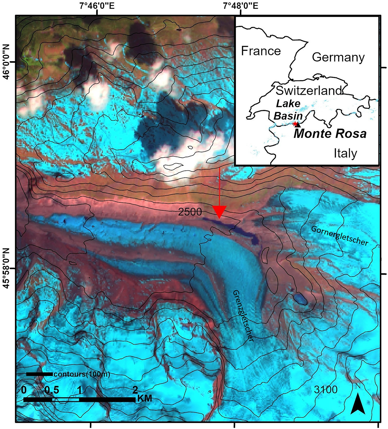
The position of the new lake between the margin of Grenzgletscher and the terminus of Gornergletscher in Monte Rosa Massif is shown on the Sentinel-2 image from 19 May 2022, when the lake had the highest detected water level. The RGB composite SWIR1–NIR–Green (Band 11-Band 8-Band 4) is used to allow a better distinction between glaciers and clouds.

Figure 1 Long description
The map depicts the Monte Rosa Massif, highlighting the position of a lake basin between the Grenzgletscher and Gornergletscher glaciers. An inset map shows the location relative to France, Germany, Switzerland and Italy. Contour lines are marked with elevation values, including 2500 and 3100 meters. The map includes a scale bar indicating distances up to 2 kilometers. Coordinates are provided along the top and left edges, with longitude ranging from 7°46′0”E to 7°48′0”E and latitude from 45°56′0”N to 45°57′0”N. A red arrow points to the lake basin area, emphasizing its location. The map uses contour lines labeled as ′contours 50 m′ to represent elevation changes and a directional arrow in the bottom right corner indicates north.
Monte Rosa has a harsh high-alpine environment, with prolonged snowfall seasons and mean annual air temperatures that are usually below freezing. The average monthly temperature at Gornergrat, located at an altitude of 3089 m a.s.l. and ∼0.8 km from the lake, ranges from ∼−8 °C in winter to ∼5–8 °C in summer, according to weather observations (Haberkorn and others, Reference Haberkorn2021). The annual precipitation is over 1200 mm, with most of it accumulating as snow between 2800 and 3000 m a.s.l. Satellite observations and field studies have shown retreating glacier tongues and rising equilibrium line altitudes (ELA) in the Monte Rosa Massif ranging from ∼3230 to 3570 m in recent years (Kropáček and Mehrishi, Reference Kropáček and Mehrishi2024). Warming trends have been observed not only at the Earth’s surface but also deep within glacier interiors, indicating that the impacts of climate change extend beyond surface melting alone (Hoelzle and others, Reference Hoelzle, Darms, Lüthi and Suter2011).
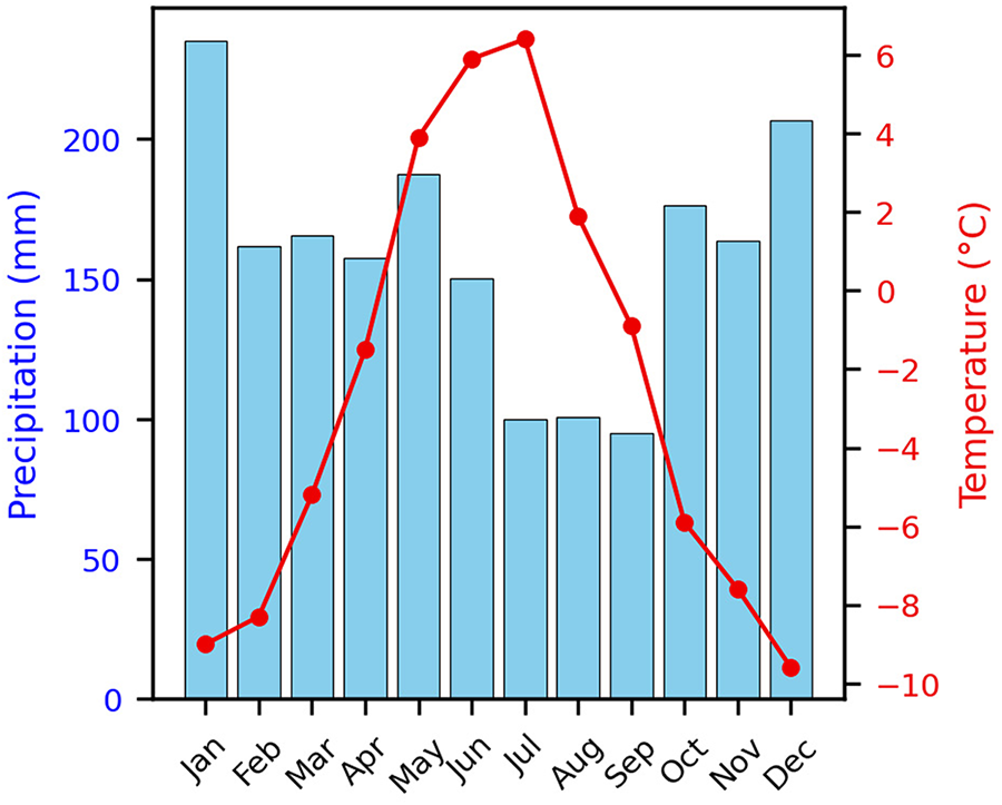
The climatograph based on the European Observation Dataset (E-OBS) (Fig. 2) shows a high variation of mean monthly temperature throughout the year with the peak in mean temperature in June and July. Precipitation is relatively evenly distributed in the year with a maximum in December and January.
Monthly temperature and precipitation patterns shown on a climatograph, illustrating seasonal variation across the basin from European Observation dataset (2016–22).

2.1 Monte Rosa and glacial lakes formed in the past
Monte Rosa has a notable history of outburst floods from Gornersee on the western side of the massif and from supraglacial lake Effimero, which forms on Belvedere Glacier, and from Locce Lake on its eastern side. The west side of the massif is drained by the Gornergletscher system, which covers an area of almost 50 km2 and has a central flow line that is 12 km long, making it one of the largest European glaciers (Sugiyama and others, Reference Sugiyama, Bauder, Riesen and Funk2010). Numerous glaciological studies have demonstrated that the mass balance of the Gornergletscher system remained unchanged between the 1930s and the early 1980s (Huss and others, Reference Huss, Hock, Bauder and Funk2012). Since then, the average annual temperature has increased, causing a negative surface mass balance that has led to a substantial decline in the Gornergletscher system (Huss and others, Reference Huss, Hock, Bauder and Funk2012). This decline is linked to an increase in local average yearly temperature, causing the ELA to rise. The Gornergletscher system includes several glacier bodies that have disconnected in the recent years, leaving former tributaries Grenzgletscher and Gornergletscher separated (Eichler and others, Reference Eichler, Legrand, Jenk, Preunkert, Andersson, Eckhardt, Engardt, Plach and Schwikowski2023).
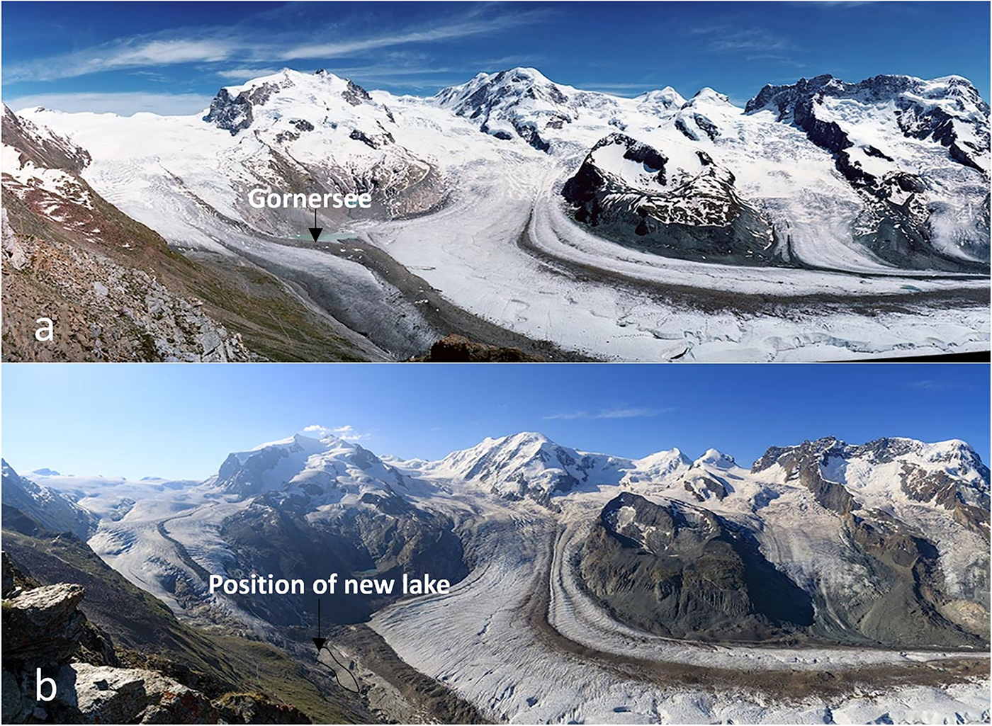
In spring 2022, the new lake formed on the western side of the mountain at the site of the former confluence of Gornergletscher and Grenzgletscher (Pandey and Kropáček, Reference Pandey and Kropáček2023) (Fig. 3). The lake growth could be traced on satellite images from mid-April to 19 May, and then it drained within a few days. This study presents a continuation of our previous work on the lake basin.
(a) The upper part of Gornergletscher on a photograph from 2004 with Gornersee visible, (b) repeat photograph from 2018 showing the position of the basin where the new lake formed in 2022. The upper part of Gornergletscher separated from the glacier system and a basin at the former confluence developed, which hosted the new short-lived lake. The photographs were provided by Jürg Alean, Eglisau.

The new lake is located near the frequently studied former glacial lake, Gornersee (Fig. 3). Gornersee was an ice-marginal lake that periodically appeared at the confluence of Gornergletscher and Grenzgletscher. It was filled with meltwater every spring and drained in early summer in a flood-like manner until 2011. It is one of the few glacial lakes in the Alps that formed and vanished in such a manner. While similar phenomena occur at other glaciers, Gornersee provided an ideal case study due to its regular drainage recurrence (Riesen and others, Reference Riesen, Strozzi, Bauder, Wiesmann and Funk2011). This spontaneous emptying was first documented in 18th century historical texts. The drainage volume reached 6 × 10⁶m3 by the end of the 1960s (Bezinge and others, Reference Bezinge, Perreten and Schafer1973; Huss and others, Reference Huss, Bauder, Werder, Funk and Hock2007). Since the 1950s, there has been a shift in the timing of drainage from August to early June, although there was no trend in the drainage volume (Huss and others, Reference Huss, Bauder, Werder, Funk and Hock2007). The lake primarily drained sub-glacially, leading to an uplift of the glacier surface and changes in glacier flow, except for one event where drainage occurred superficially with no impact on glacier flow (Riesen and others, Reference Riesen, Strozzi, Bauder, Wiesmann and Funk2011).
The new lake shares at least part of its drainage basin with the former Gornersee whose volume oscillated in the range of 1–5 × 10⁶ m3 (Huss and others, Reference Huss, Bauder, Werder, Funk and Hock2007). In terms of area, the lake is comparable with the former Gornersee (Pandey and Kropáček, Reference Pandey and Kropáček2023).
3. Materials and methods
3.1 Fieldwork
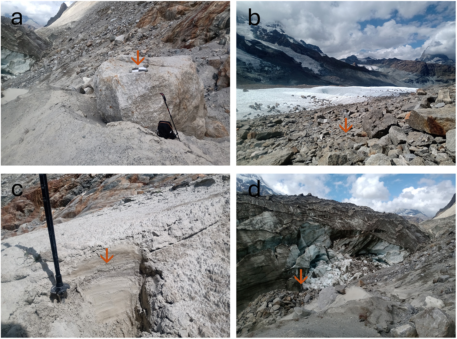
Fieldwork at the drained lake basin was conducted on 5–6 August 2023, ∼1 year after the drainage, to validate remote-sensing interpretations and carry out UAV flight supported with ground control (Fig. 4a). We investigated the general setting of the lake bordered by a moraine (Fig. 4b). We could identify distinct drainage patterns that remained well preserved even with a 1-year lag. We investigated the drainage feature in the basin in terms of active and non-active inflows, supraglacial drainage, outlets from the basin and depositional features (Fig. 4c). Furthermore, we could investigate the zone of contact between the glacier and bedrock (Fig. 4d). The field observations allowed us to refine our previous assumptions based solely on remote-sensing data. For instance, contrary to the previous interpretations, we confirmed that the lake had direct contact with the glacier ice.
Features identified during the fieldwork: (a) Control point on a stable Boulder marked by a square chess pattern plate; (b) Former medial moraine along the southern edge of the basin and the tongue of Grenzgletscher; (c) Deposit of lacustrine sediment in the lake basin; and (d) Margin of the glacier with potential subglacial inflow.

3.2 Acquisition and processing of UAV data
In August 2023, a UAV field campaign was conducted to acquire data for 3-D reconstruction of the lake basin. A DJI Mavic drone equipped with a Hasselblad RGB CMOS 1/2.3” camera (focal length: 28 mm; image resolution: 4000 × 3000 pixels) was used for the campaign. A total of 2198 digital images were captured over the lake basin with ∼70% forward overlap between consecutive images along each flight line and 70% side overlap between adjacent flight lines. The UAV flew at an altitude of 100 m above ground level, resulting in a ground sampling distance of ∼3.2 cm.
Prior to the acquisitions, nine fixed 50 × 50 cm polypropylene plates with a chessboard pattern were placed on stable terrain and accurately surveyed using a high-precision R12i Global Navigation Satellite System by Trimble to be used later as nine ground control points (GCPs), out of which four checkpoints were selected for the error estimation and then returned and used as GCPs.
The image data were processed in Agisoft Metashape Professional version 1.6.5 photogrammetry software to generate both a digital surface model (DSM) and an orthomosaic of the study area, following the standard workflow with default settings for image alignment. After image alignment, a dense point cloud was created, providing a highly detailed and realistic 3-D representation of the surface topography.
The aligned images and dense point cloud were carefully reviewed and cleaned to remove noise and erroneous points. Using the processed dense cloud, a high-resolution surface mesh was constructed to accurately represent the terrain. The mesh was then converted into a raster format to build the DSM, ensuring that the model captured the true surface elevations of the study area (Fig. 5). Finally, the DSM was georeferenced and exported in a standard projection system (UTM zone 32, WGS_84) for integration with other spatial datasets, with Sentinel-2 images.
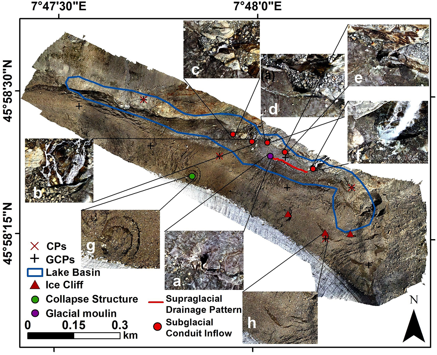
The orthomosaic, based on UAV photographs showing drainage features in the basin such as glacier moulin, subglacial conduit inflows and supraglacial streams. The maximum lake extent on 19 May 2022 and ground control points are shown. In detail figures, the following features are shown: moulin, (a–f) inflows, (g) collapse structure and (h) ice cliff.

Figure 5 Long description
The orthomosaic map displays drainage features in a basin, marked with various symbols. Key features include glacier moulin (green circle), subglacial conduit inflows (red dots) and supraglacial drainage patterns (blue line). The map also highlights a lake basin (blue outline), ice cliffs (blue triangles) and a collapse structure (purple circle). Ground control points (GCPs) are marked with plus signs and control points (CPs) with red crosses. Insets labeled a to h provide detailed views of specific features: a) glacier moulin, b-f) inflows, g) collapse structure and h) ice cliff. The scale bar indicates distances from 0.15 to 0.3 kilometers. The map is oriented with north at the top and coordinates are provided along the edges.
As illustrated in Fig. 5, the DSM provides a high-resolution visual representation of the basin and its geomorphological structures facilitating interpretation of spatial patterns, key drainage and surface changes over time.
To assess the accuracy of the mapping, the root mean square error (RMSE) was calculated to quantify the average deviation between the mapped and source coordinates of the check points. RMSE provides a single measure of the magnitude of errors and is widely used in positional accuracy assessment. The RMSE was calculated separately for the horizontal (X and Y) and vertical (Z) residual components, as well as combined into two-dimensional (2-D) and 3-D error metrics. The horizontal (X) RMSE was 3.27 m, the horizontal (Y) RMSE was 1.43 m, and the vertical (Z) RMSE was 1.43 m. The combined 2-D RMSE (horizontal plane) was 3.57 m, and the combined 3-D RMSE (including the vertical component) was 3.85 m, indicating a slightly higher positional error in the horizontal direction.
3.3 Analysis of satellite data
For the investigation of the lake evolution, we utilized Sentinel-2 data, specifically the L2A products with atmospherically corrected reflectance values (Drusch and others, Reference Drusch2012). Sentinel-2 is a constellation of two identical satellites operated by the European Space Agency as part of the Copernicus program of the European Commission. Its Multispectral Instrument captures information about the land surface in 12 spectral bands, encompassing the visible, near-infrared (NIR) and shortwave infrared (SWIR) portions of the electromagnetic spectrum. This capability facilitates the differentiation between glaciers, snow (distinct from clouds) and water bodies. The high spatial resolution (10 m for four bands) provides a sufficient level of detail to map glacial lakes (e.g. Wangchuk and Bolch, Reference Wangchuk and Bolch2020). The application of Sentinel-2 imagery in high-mountain regions can be partially hindered by snow and cloud cover, as well as by deep shadows caused by high relief. These challenges can be mitigated to some extent by using multispectral methods such as band ratios and SWIR (Jiang and others, Reference Jiang, Ni, Pang, He, Fu, Lu, Yang, Long and Lei2020; Pandey and others, Reference Pandey, Rai, Gupta, Shukla and Dimri2021).
We used Sentinel-2 images for mapping the lake extent (Table 1). In cases where lake presence was obscured by cloud cover, we explored Sentinel-1 SAR imagery. However, radar data failed to confirm the lake’s presence, likely due to wind effects on the lake surface resulting in similar backscatter to the surrounding areas. For the mapping of lake extent, we used initially the Normalized Difference Water Index, but a difficult separation of water and ice led to an overestimation of water extent. Therefore, a band ratio of green (B3) and NIR (B8) was used to delineate lake extent, applying a threshold of green/NIR > 1.5 (Pandey and others, Reference Pandey, Rai, Gupta and Shukla2017). Area uncertainty is primarily associated with mixed pixels along the land–water boundary, where raster representation prevents precise delineation of the shoreline. The uncertainty in lake area was therefore estimated using a resolution-based approach that accounts for boundary pixel effects (Burrough and McDonnell, Reference Burrough and McDonnell1998; Jensen, Reference Jensen2005).
List of used Sentinel-2 images.

Table 1 Long description
The table lists Sentinel-2 image acquisition dates grouped by how they were used for lake analysis. One group includes five images from late April through late May 2022, used for both area estimation and measuring lake extent. The other group includes three images dated 20 May 2017, 12 May 2018, and 14 May 2022, used for lake area estimation only. The extent measurement work relies solely on 2022 imagery and uses more dates than the area-only group. Area estimation draws on a wider time span across multiple years, but with fewer images. Dates are provided without additional details such as location, cloud cover, or processing steps, which may affect how comparable results are across acquisitions.
Furthermore, we used very-high resolution (VHR) images on Google Earth from December 2016, February 2017, April 2017, December 2018 and October 2019 to get more insight into the lake basin evolution prior to the lake formation in 2022.
3.4 Calculating the volume
To estimate the volume of the drained lake, a DSM of the exposed lakebed was combined with the pre-drainage lake extent. A flat water-level raster representing the maximum lake surface elevation was first generated, and the DSM elevation was subtracted from this surface to derive spatially distributed water depth. Only positive depth values, corresponding to inundated areas, were retained, while zero or negative values were excluded. The lake volume was then calculated by summing the product of depth and pixel area across the lakebed. To account for post-drainage morphological changes, visible drainage features, including channels and moulins, were delineated as shapefiles from the orthomosaic. A continuous pre-drainage lakebed surface was approximated by interpolating across these features using the nearest stable surrounding contours, and their depths were estimated relative to adjacent undisturbed morphology. The volume associated with these features was quantified and subtracted from the initial estimate to obtain a corrected lake volume representative of pre-drainage conditions. Similarly, we calculated the lake volume for each stage of filling and drainage captured by Sentinel-2 data. The resulting volumes were further compared with estimates derived from widely used empirical area–volume relationships proposed by Huggel and others (Reference Huggel, Kääb, Haeberli, Teysseire and Paul2002), Cook and Quincey (Reference Cook and Quincey2015) and Watson and others (Reference Watson, Quincey, Carrivick, Smith, Rowan and Richardson2018), which express lake volume as a function of surface area (Table 2).
Summary of empirical area–volume relationships used for estimating lake volumes.

Table 2 Long description
The table summarizes three empirical relationships used to estimate lake volume from lake surface area. Two relationships are intended for worldwide use: one for moraine and ice-dammed lakes and one for supraglacial lakes. A third relationship is specific to the Himalaya and applies to supraglacial lakes. The moraine and ice-dammed relationship implies larger volume estimates for a given area than the worldwide supraglacial relationship. For supraglacial lakes, the Himalaya-specific relationship implies higher volumes for a given area than the worldwide supraglacial relationship. References are provided for each relationship, including Huggel and others, Cook and Quincey, Watson and others, and Zhang and others. These relationships are empirical and their accuracy depends on using them within the stated region and lake-type conditions.
Note: Each formula expresses volume (V, in million cubic meters) as a function of lake surface area (A, in km2).
3.5 Analysis of temperature and precipitation data
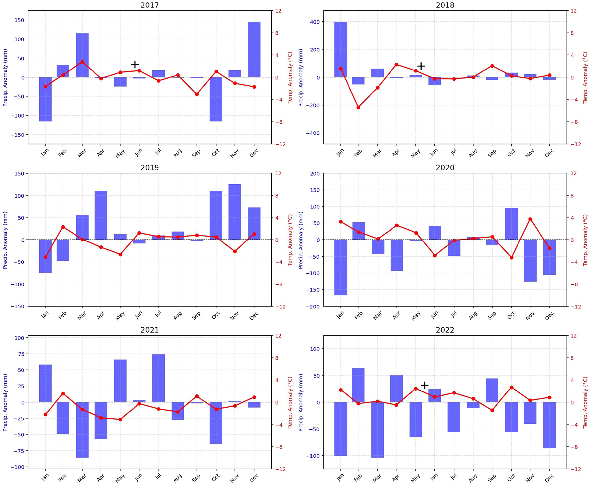
To assess the potential influence of local climatic variability on the lake presence, a comparative analysis of temperature and precipitation data was conducted utilizing an assembled gridded daily meteorological E-OBS dataset from the European Climate Assessment and Dataset project network with a resolution of 0.1 degrees (Cornes and others, Reference Cornes, van der Schrier, van den Besselaar EJM and Jones2018). Monthly mean precipitation values were computed to evaluate differences in rainfall patterns, while both mean and maximum temperature values were derived to capture variations in thermal conditions. The analysis primarily focused on the months of April, May and June, as these represent the active period associated with lake formation in late spring. Data from lake years (2017, 2018 and 2022) were compared with no-lake years (2019, 2020 and 2021). Subsequently, the mean of the maximum temperatures for each category was calculated to examine potential differences. This approach enabled the identification of possible climatic drivers linked to the presence or absence of the lake. Furthermore, the anomalies of monthly temperature and precipitation from the mean were calculated.
4. Results
4.1 Properties of the lake
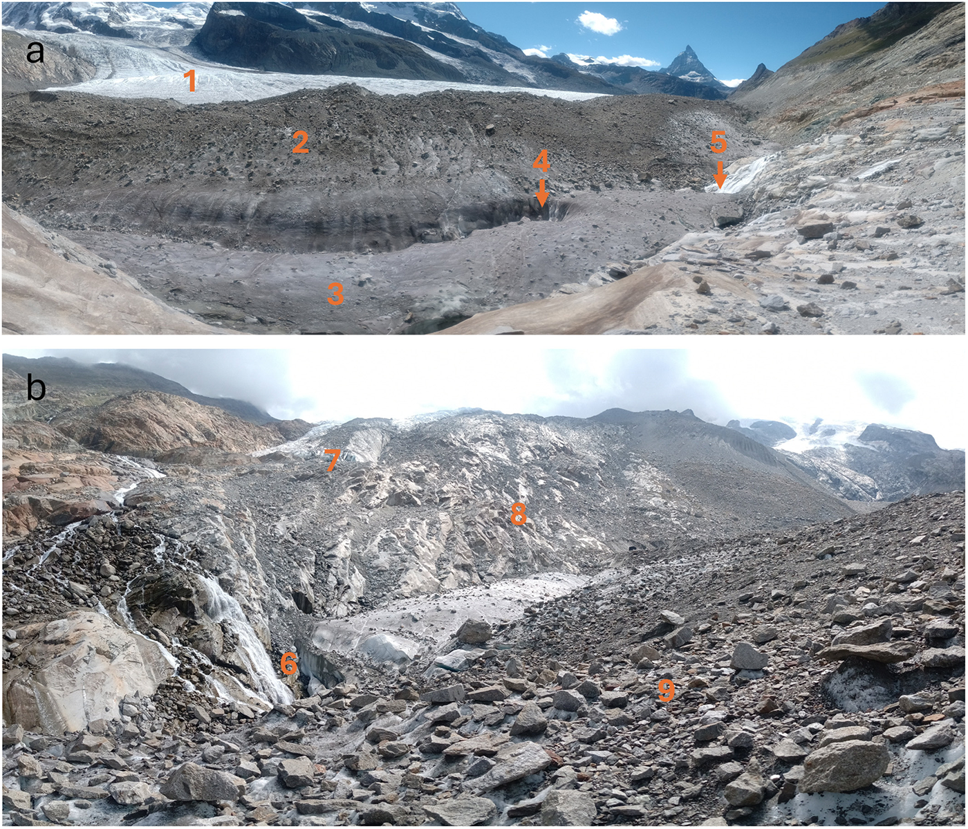
The lake formed on the former confluence of Gornergletscher and Grenzgletscher, which featured a medial moraine at an elevation of 2536 m a.s.l. The lake filled an elongated basin between the moraine on the Grenzgletscher and a rocky slope dividing the present terminus of Gornergletscher, which is located at an altitude of 2590 m a.s.l. (Fig. 6). Based on a Sentinel-2A image acquired on 14 May 2022, the lake reached ∼1.13 km in length and covered an area of 0.08 ± 0.024 km2.
(a) Panorama photograph of the empty lake basin from the North taken on 5 Aug 2023. It shows Grenzgletscher flowing to the right (1), the moraine forming the southern side of the basin (2), the ice surface of the Gornergletscher’s margin (3), a glacier moulin (4) and inflow of a stream from Gornergletscher (5). (b) The view of the basin from the west shows: subglacial inflow entering below the Grenzgletscher (6), disconnected Gornergletscher (7), loose debris material (8), moraine (9).

4.2 Evolution and drainage of the lake
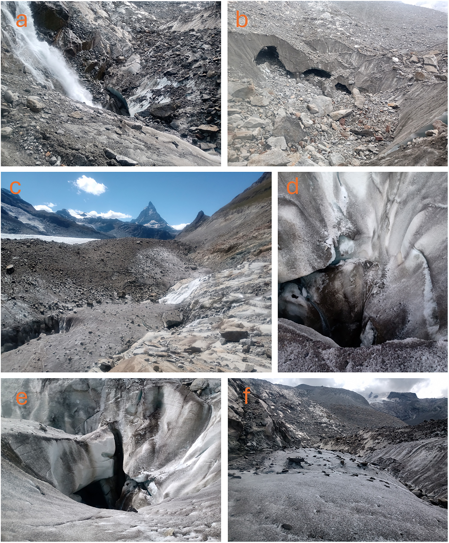
After a period of complete cloud cover, the lake was observed in satellite images on 26 April 2022 as a group of small water ponds. The lake had an elongated shape and grew steadily from the second half of April, extending toward the northwest. The lake began forming in deeper areas, fed initially by clean snowmelt from inflow channels (Fig. 7a and c). The inflow from portals in the east side or the lake basin was probably already inactive (Fig. 7b). By 29 April, the western part turned turbid due to sediment-rich inflow. This is consistent with fine-grained, laminated silt clay sediments documented during the fieldwork, indicative of gradual deposition under calm subaqueous conditions (Fig. 4c). The lake reached full extent (0.1 ± 0.029 km2) at the elevation of 2443.9 m a.s.l. on 19 May and was drained on 26 May (Pandey and Kropáček, Reference Pandey and Kropáček2023).
Drainage features in the empty lake basin: (a) First Inflow to the basin from Gornergletscher; (b) Inactive inflow portals into the basin on its eastern side; (c) Western part of the basin with moraine superimposed on the glacier, a glacier moulin and second inflow from Gornergletscher; (d and e) Glacier moulin; and (f) an inactive drainage channel forming the deepest part of the basin.

A thorough check of Sentinel-2 data revealed that the lake appeared already before 2022 but with a smaller area. On 20 May 2017, the area of the lake was 0.015 ± 0.014 km2, while on 20 May 2018 the area was 0.012 ± 0.030 km2. The smaller pond can be seen on Sentinel-2 L2A satellite imagery of 4 June 2019 with an area of 0.014 ± 0.0042 km2. According to the report of the Swiss Alpine Association, the lake rendered the access trail to Monte Rosa Hut difficult to maintain (Section Monte Rosa, 2026). This led eventually to the construction of an alternative access trail crossing Gornergletscher at higher elevation in 2019. The check of VHR images available in Google Earth platform showed that the supraglacial drainage channel (Figs 5 and 6) existed already in 2016 and only slightly changed in the period 2016–19. The subglacial conduit with inflow from Gornergletscher (Fig. 5b) was active already in 2017. The glacier moulin, however, could be identified only on the orthoimage from 2023. The presence of the drainage features in the basin detected both in VHR images and during the fieldwork indicates that the drainage of the lake was subglacial, through the glacier moulin and a subglacial conduit (Fig. 7d and e).
4.3 Lake volume
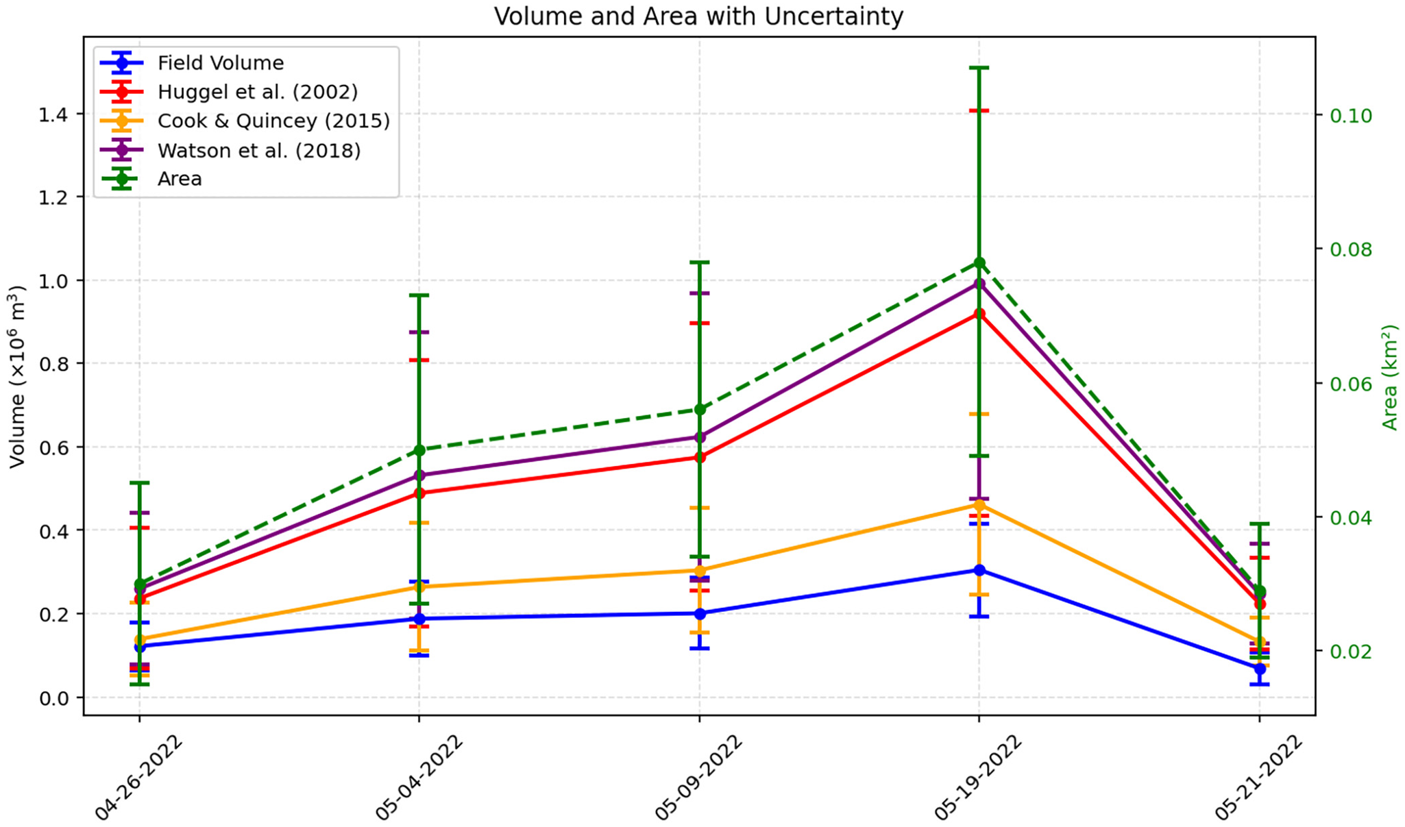
The DEM of the empty basin allowed us to calculate lake volumes for five lake filling stages, given by the available cloud-free satellite images. The comparison of the calculated volumes with volumes derived by the three empirical formulas is shown in (Fig. 8). The comparison of modeled and field-derived volumes shows that all three formulations exhibit a tendency to deviate from measured values, though to varying degrees. The relationship proposed by Cook and Quincey (Reference Cook and Quincey2015) results in an average difference of ∼50%, with a general tendency toward overestimation. In comparison, the approaches of Huggel and others (Reference Huggel, Kääb, Haeberli, Teysseire and Paul2002) and Watson and others (Reference Watson, Quincey, Carrivick, Smith, Rowan and Richardson2018) show substantially larger deviations, consistently overestimating lake volume by ∼76% and 100%, respectively. These differences show the challenges when employing empirical formulas without local calibration and emphasize the significance of field bathymetry measurements.
Comparison of the lake volumes based on the UAV-based DEM and the lake extents derived from satellite data, with estimates from three empirical area–volume formulas: Huggel and others (Reference Huggel, Kääb, Haeberli, Teysseire and Paul2002), Cook and Quincey (Reference Cook and Quincey2015) and Watson and others (Reference Watson, Quincey, Carrivick, Smith, Rowan and Richardson2018).

Figure 8 Long description
Volume and Area with Uncertainty. Legend: Field Volume; Huggel et al. (2002); Cook and Quincey (2015); Watson et al. (2018); Area. All listed series rise from 04-26-2022 to 05-15-2022 and then drop on 05-21-2022. On each date, Watson et al. (2018) is higher than Huggel et al. (2002) and both are higher than Cook and Quincey (2015) and Field Volume. Field Volume is the lowest volume series on all dates. The highest volume value occurs on 05-15-2022 for Watson et al. (2018) at 1.00 and the lowest volume value occurs on 05-21-2022 for Field Volume at 0.08. Area reaches its highest value on 05-15-2022 at 0.075 and its lowest value on 05-21-2022 at 0.03. Horizontal axis label: Date. Horizontal axis values: 04-26-2022, 05-04-2022, 05-09-2022, 05-15-2022, 05-21-2022. Left vertical axis label: Volume (times 10 superscript 6 m superscript 3). Left vertical axis range: 0.0 to 1.4. Right vertical axis label: Area (km superscript 2). Right vertical axis range: 0.02 to 0.10. Field Volume coordinate pairs: (04-26-2022, 0.12), (05-04-2022, 0.18), (05-09-2022, 0.19), (05-15-2022, 0.30), (05-21-2022, 0.08). Huggel et al. (2002) coordinate pairs: (04-26-2022, 0.20), (05-04-2022, 0.50), (05-09-2022, 0.58), (05-15-2022, 0.95), (05-21-2022, 0.18). Cook and Quincey (2015) coordinate pairs: (04-26-2022, 0.15), (05-04-2022, 0.25), (05-09-2022, 0.30), (05-15-2022, 0.45), (05-21-2022, 0.12). Watson et al. (2018) coordinate pairs: (04-26-2022, 0.22), (05-04-2022, 0.55), (05-09-2022, 0.62), (05-15-2022, 1.00), (05-21-2022, 0.20). Area coordinate pairs: (04-26-2022, 0.03), (05-04-2022, 0.05), (05-09-2022, 0.055), (05-15-2022, 0.075), (05-21-2022, 0.03).
4.4 Weather conditions related to lake formation
The winter of 2021–22 was exceptional in the southern Alps. According to the Swiss Meteo periodic report, it ranked as the second mildest, sunniest and second driest winter since records began in 1864. Precipitation was notably sparse in southern Switzerland between December 2021 and March 2022, leading to limited snow accumulation. February temperatures exceeded the 1991–2020 mean by ∼2°C across Switzerland, further contributing to the snow deficit. Subsequently, a low-pressure system moving from southern France on 23 April produced intense precipitation up to 100 mm d−1 in southern Switzerland, with fresh snow depths reaching 30–70 cm. A second episode of rainfall associated with a cold front occurred on 30 April. The meltwater generated from this late-season snow accumulation rapidly filled the lake basin. Temperature records from the Monte Rosa Hut (2883 m a.s.l.), located 2.1 km from the lake, indicated daily means between 3.4°C and 9.4°C from 12 to 18 May (Windfinder, 2022), providing favorable conditions for accelerated snowmelt and filling of the lake basin.
Figure 9 presents the temperature and precipitation anomalies for both lake and no-lake years based on the E-OBS dataset. All lake years show positive thermal anomalies during the key lake-formation period (April–June). In 2017, temperature anomalies are positive in May and June, with a particularly strong anomaly in March; in 2018, positive anomalies occur in April and May; and in 2022, a positive anomaly is observed only in May. In contrast, the no-lake years 2019 and 2021 exhibit negative temperature anomalies in April and May, while 2020, also a no-lake year, shows a strong positive anomaly in the same months. This indicates that high temperatures alone do not guarantee lake formation and that local basin conditions lead to lake formation.
The monthly temperature and precipitation anomalies based on the European Observation dataset for the period 2017–22 showing the various conditions of the lake formation period. The observed lake presence in the basin is indicated by a plus above the X-axis.

Figure 9 Long description
The image A showing 2017. Text: 2017. The horizontal axis shows months: Jan, Feb, Mar, Apr, May, Jun, Jul, Aug, Sep, Oct, Nov, Dec. The left vertical axis label: Temperature anomaly (degree celsius). Range: negative 3.0 to 3.0. The right vertical axis label: Precipitation anomaly (millimeter). Range: negative 12 to 12. A bar series is plotted for temperature anomaly and a line series is plotted for precipitation anomaly. The precipitation anomaly line starts near 0 in Jan, rises to a local high around Mar, then stays near 0 from Apr through Aug, drops below 0 around Sep, rises near 0 around Oct and ends below 0 in Nov and Dec. The temperature anomaly bars include a negative bar in Jan, positive bars in Feb and Mar, small bars near 0 from Apr through Aug, a negative bar in Sep, a positive bar in Oct and a tall positive bar in Dec. A plus symbol is plotted above the horizontal axis near May. The image B showing 2018. Text: 2018. The horizontal axis shows months: Jan, Feb, Mar, Apr, May, Jun, Jul, Aug, Sep, Oct, Nov, Dec. The left vertical axis label: Temperature anomaly (degree celsius). Range: negative 3.0 to 3.0. The right vertical axis label: Precipitation anomaly (millimeter). Range: negative 12 to 12. A bar series is plotted for temperature anomaly and a line series is plotted for precipitation anomaly. The precipitation anomaly line is above 0 in Jan, drops to a low below 0 in Feb, rises above 0 in Mar and Apr, then stays close to 0 from May through Dec with small rises around Sep and Oct. The temperature anomaly bars include a tall positive bar in Jan, negative bars in Feb and Mar and small bars near 0 from Apr through Dec. A plus symbol is plotted above the horizontal axis near May. The image C showing 2019. Text: 2019. The horizontal axis shows months: Jan, Feb, Mar, Apr, May, Jun, Jul, Aug, Sep, Oct, Nov, Dec. The left vertical axis label: Temperature anomaly (degree celsius). Range: negative 3.0 to 3.0. The right vertical axis label: Precipitation anomaly (millimeter). Range: negative 12 to 12. A bar series is plotted for temperature anomaly and a line series is plotted for precipitation anomaly. The precipitation anomaly line is above 0 in Jan, then trends downward toward 0 by Mar, dips below 0 around Apr and May, then stays close to 0 from Jun through Oct and rises above 0 in Nov and Dec. The temperature anomaly bars include a negative bar in Jan, positive bars in Feb and Mar, small bars near 0 from Apr through Aug and multiple tall positive bars from Sep through Dec. The image D showing 2020. Text: 2020. The horizontal axis shows months: Jan, Feb, Mar, Apr, May, Jun, Jul, Aug, Sep, Oct, Nov, Dec. The left vertical axis label: Temperature anomaly (degree celsius). Range: negative 3.0 to 3.0. The right vertical axis label: Precipitation anomaly (millimeter). Range: negative 12 to 12. A bar series is plotted for temperature anomaly and a line series is plotted for precipitation anomaly. The precipitation anomaly line starts above 0 in Jan, declines toward 0 by Mar, dips below 0 around May, rises above 0 around Jun and Jul, stays near 0 around Aug and Sep, drops below 0 around Oct, rises above 0 around Nov and ends near 0 in Dec. The temperature anomaly bars include a large negative bar in Jan, positive bars in Feb and Mar, negative bars in Apr and May, small bars near 0 in Jun and Jul, a positive bar in Sep, a negative bar in Oct, a positive bar in Nov and a negative bar in Dec. The image E showing 2021. Text: 2021. The horizontal axis shows months: Jan, Feb, Mar, Apr, May, Jun, Jul, Aug, Sep, Oct, Nov, Dec. The left vertical axis label: Temperature anomaly (degree celsius). Range: negative 3.0 to 3.0. The right vertical axis label: Precipitation anomaly (millimeter). Range: negative 12 to 12. A bar series is plotted for temperature anomaly and a line series is plotted for precipitation anomaly. The precipitation anomaly line is near 0 in Jan, rises above 0 in Feb, drops below 0 in Mar and Apr, stays below 0 around May and Jun, rises toward 0 around Jul, rises above 0 around Aug, dips below 0 around Sep and ends above 0 around Nov and Dec. The temperature anomaly bars include a positive bar in Jan, negative bars in Feb and Mar, positive bars in Apr and May, small bars near 0 in Jun and Jul, a negative bar in Sep and small bars near 0 in Oct through Dec. The image F showing 2022. Text: 2022. The horizontal axis shows months: Jan, Feb, Mar, Apr, May, Jun, Jul, Aug, Sep, Oct, Nov, Dec. The left vertical axis label: Temperature anomaly (degree celsius). Range: negative 3.0 to 3.0. The right vertical axis label: Precipitation anomaly (millimeter). Range: negative 12 to 12. A bar series is plotted for temperature anomaly and a line series is plotted for precipitation anomaly. The precipitation anomaly line is near 0 in Jan, dips below 0 in Feb, rises above 0 in Mar and Apr, stays near 0 around May and Jun, dips below 0 around Jul, rises above 0 around Aug, dips below 0 around Sep, rises above 0 around Oct and ends near 0 in Nov and Dec. The temperature anomaly bars include positive bars in Jan, Mar and Apr, negative bars in May, Jun and Jul, a positive bar in Aug and negative bars in Sep, Oct and Dec. A plus symbol is plotted above the horizontal axis near May.
Precipitation patterns further support this interpretation. Although the 2017–22 E-OBS data reveal substantial interannual variability in maximum daily precipitation, there is no consistent relationship with lake occurrence. Lake years experienced several moderate to high precipitation events in April and May, but overall precipitation magnitude and frequency were similar to those of no-lake years. In terms of anomalies, both 2017 and 2018 show predominantly negative precipitation anomalies during April–June, apart from a slightly positive anomaly in May 2018. In 2022, precipitation fluctuated strongly, producing alternating positive and negative anomalies; within the lake-formation period, May showed a strong negative anomaly, while April contained the late-month precipitation event noted earlier and June showed positive anomalies. No-lake years also exhibit large precipitation variability, especially in 2021. These patterns indicate that precipitation alone was not a determining factor for lake formation; rather, its timing and interaction with snowpack and melt conditions likely influenced the lake formation.
The temperature data for lake years indicate relatively strong and sustained warm periods, particularly in late spring. Mean maximum temperatures in April, May and June during lake years were distinctly higher 2.71°C, 3.47°C and 2.08°C, compared to 0.79°C, 2.03°C and −1.1°C in the no-lake years (2019–21). Consistently higher mean temperatures were also observed in lake years (T m = 2.75°C) relative to no-lake years (T m = 0.57°C) supporting the conclusion that lake years were generally warmer than no-lake years.
5. Discussion
5.1 The recurrent nature of the new lake
The repeated formation of this short-lived lake represents a recurrent phenomenon, related to both global warming and very local morphological and drainage conditions. There are several notable examples of recurrent floods from glacier-marginal lakes in the Alps that have required technical measures to mitigate their hazard potential. Märjelensee, a large glacier-marginal lake at Grosser Aletschgletscher, drew considerable attention due to its devastating outburst floods throughout the 19th century. The lake’s volume was ∼1 × 10⁶ m3, and its drainage took between 3 and 7 days (Preller, Reference Du Riche Preller1896). It usually drained englacially and, in some years, supraglacially (Schweizer, Reference Schweizer1957). The tunnel constructed in 1895 to control the lake level soon became obsolete as the lake level fell below the tunnel inflow due to glacier downwasting.
A more recent example is the recurrent drainage of the glacier-marginal lake Faverges at Plaine Morte Glacier in the Swiss Alps. This lake, which has drained annually since 2011, reached more than 2 × 10⁶ m3 in the summer of 2018 and drained within 24 hours on 27 July 2018, causing damage in the downstream village of Lenk (Ogier and others, Reference Ogier, Werder, Huss, Kull, Hodel and Farinotti2021). As a flood prevention measure, an 800 m-long channel combined with a short tunnel was constructed in spring 2019 to drain the lake across the glacier toward the west. However, the channel became blocked by snow during the subsequent winter, requiring further technical measures.
Some glaciers can produce dangerous glacial lake outbursts even after long periods of dormancy (Vincent and others, Reference Vincent, Descloitres, Garambois, Legchenko, Guyard and Gilbert2012). In 1892, a sudden outburst from a subglacial lake beneath the Tête Rousse Glacier in Mont Blanc Massif, France, caused a devastating flood that caused 170 casualties in the village of Saint-Gervais (Vincent and others, Reference Vincent, Garambois, Thibert, Lefebvre, Le Meur and Six2010). The lake reappeared in recent years, and in 2010, it was drained as a preventive measure after being detected by radar surveys.
5.2 Factors of lake appearance and drainage
The drainage on 26 May constitutes an early drainage, considering that glacier lake drainages occur typically from end of June to August. For instance, Gornersee used to drain between June and August; similarly, lake Faverges usually drains between mid-June and late August, depending on meltwater accumulation and drainage channel formation (Ogier and others, Reference Ogier, Werder, Huss, Kull, Hodel and Farinotti2021). Märjelensee (Aletschgletscher) experienced periodic outbursts; except for a notable event in January 1883, all documented events occurred between June and October. These summer outbursts were especially frequent during periods when the glacier was at its maximum extent (Haeberli, Reference Haeberli1983). Summer temperature and precipitation are frequently discussed in connection with the formation and drainage of glacial lakes. In the case of the new lake, weather records indicate that after winters with minimal precipitation, late-April snow accumulation associated with passing frontal systems can contribute substantially to lake inflow. In Gornersee, temperature-index melt models and runoff simulations showed that warm spring and early-summer temperatures increase meltwater input, and field observations confirm subglacial drainage once critical pressures are reached (Huss and others, Reference Huss, Bauder, Werder, Funk and Hock2007). In the case of lake Faverges, the filling is largely dominated by melt rather than precipitation, and drainage occurs via supraglacial channels during sustained summer melting (Ogier and others, Reference Ogier, Werder, Huss, Kull, Hodel and Farinotti2021). Historical outburst events at Märjelensee occurred under conditions of gradually increasing temperatures, suggesting that long-term warming trends may have generally favored melt-driven hydrology (Du Riche Preller, Reference Du Riche Preller1896; Schweizer, Reference Schweizer1957). Overall, these cases suggest a recurring scenario in which above-average early summer melt following winters with low snowfall drives the formation of short-lived lakes, although heavy rainfall or rain-on-snow events can accelerate lake filling in some cases (Beniston and Stoffel, Reference Beniston and Stoffel2016; Hock and others, Reference Hock2019). Understanding the drainage mechanism of the new lake is essential to better assess its hazard potential. The lake likely drained via the identified glacier moulin or the subglacial conduits located along the margin of the glacier. Further, the drainage followed sub- or englacial drainage paths. Surface drainage along the glacier margin cannot be excluded but is not likely considering the drainage features at the basin’s bottom. It should be noted that the outburst mechanisms of even well-studied lakes such as Gornersee are not completely understood and remain subject to many uncertainties (Bauder and others, Reference Bauder2008).
The possible outflow from the basin during the fieldworks in 2023 was via conduits at the bottom of the basin and along the boundary between the ice and rock slope, suggesting a subglacial drainage (Figs 5, 6a, 7a and 6b). The outflows from the basin, including the inactive glacier moulin, could be blocked either by ice movement or filling by sediments. There is a large amount of loose debris deposited on the slopes of the basin, making the second scenario likely (Fig. 6b). A blockage of these drainage channels may prevent subglacial outflow and create the favorable conditions of lake formation in the future. According to local and regional media, the lake drainage in 2022 has not caused any damage. However, it is important to note that the discharge of Gornersee has varied significantly from year to year. Given this variability, it is recommended that the lake be monitored for its potential hazard in the event of its future reappearance. Especially in case that the vertical conduits become blocked by the debris material richly available in and around the basin (Fig. 6b), the lake can develop again, as there is plenty of inflow of meltwater from Gornergletscher enhanced by snowmelt during a sudden temperature rise.
5.3 Time lag between lake appearance and fieldwork
The 1 year lag between the appearance of a glacial lake and the subsequent fieldwork introduces several challenges. By the time of the visit, the lake basin was empty. Changes in topography, such as sediment redistribution, ice melt and glacial movement, could modify its shape and some drainage features. Additionally, shifts in drainage pathways and groundwater levels may impact the observed landscape (Winter, Reference Winter2001). Nevertheless, the check of the VHR images indicated that the changes were not substantial. At least the subglacial conduit inflow most likely existed, and the glacier moulin appeared during the drainage in 2022. The appearance of the moulin in 2023, in the year of the fieldwork, can probably be excluded, while its existence prior to 2022 remains uncertain.
6. Conclusions
We documented the formation and unusually early drainage of a new lake within the well-studied Gornergletscher system in the Swiss Alps. The ice-marginal lake basin formed at the former glacier confluence between a moraine superimposed on the glacier and a rock slope earlier covered by ice. Field evidence provided deeper insight into the drainage mechanisms. Based on UAV mapping, we reconstructed bathymetry and estimated volume of the lake over its five stages of evolution for which the delineation of the lake area was allowed by cloud-free satellite images. Estimated volumes were then compared from three widely used empirical area–volume formulas. The results show that the Cook and Quincey (Reference Cook and Quincey2015) scaling provided estimates most closely matching the field‐derived volumes, whereas the others generally overestimated, underscoring the importance of validation of these formulas by in situ data. Comparisons of temperature and precipitation for years of lake appearance (2017, 2018, 2022) and years of no-lake appearance indicate that air temperature is the dominant controlling factor, and hence the lake is likely to reappear under similar thermal conditions, provided the basin will be sealed, for instance by blockage of the outlets by debris or glacier movement.
Importantly, in this case the lake drained completely on 26 May 2022, constituting an early outburst. By contrast, many glacial lake outburst events in the Alps typically occur later in summer, July or August, when melting and hydrologic pressures peak. Taken together, these cases suggest that the lake drainage occurred significantly earlier than typical seasonal lake drainages in the region, suggesting a rare or anomalous glacial hydrological response. However, the early lake drainage of the new lake is consistent with the general shift of drainage of glacial lakes toward an earlier date.
As the glacier continues to retreat, the basin may expand, potentially increasing the risk to downstream settlements. The rapid appearance and sudden drainage of glacial lakes related to thermally driven fast snowmelt represent a threat that should also be considered in other glaciated valleys in the Alps. This also underscores the need for timely monitoring of new lake formation, especially during rapid snowmelt situations. Furthermore, newly formed concave forms at glacier margins should be focused on, as they represent a hazard due to possible fast lake formation.
Acknowledgements
We acknowledge USGS Earth Explorer and Copernicus Open Access Hub for providing open data for this work. We would like to thank Dr. Lukáš Brodský and Daniel Bicák for their help during the UAV data collection. We are grateful to Mr. Jürg Alean for providing the repeat photographs freely for this manuscript. This work was carried out in the framework of the 4EU+ Student Mini Grant entitled Collaborative research on a newly appeared glacial lake in the Alps and 4EU Project ‘Multidisciplinary approaches to estimate evolution of glacial and periglacial areas in the Alps under climate change conditions’.
Funding statement
This work was supported by the Faculty of Science, Charles University, grant: Cooperatio (COOP) and OP JAK programme ‘Natural and anthropogenic geohazards’ (CZ.02.01.01/00/22_008/0004605).
Competing interests
The authors have no relevant financial or non-financial interests to disclose.



 Open access

