





1. Introduction
Critical layers are a prominent feature of wave dynamics. They arise when the governing wave equations become singular, signifying that the physical assumptions made in deriving them – e.g. that the wave dynamics are linear and inviscid – are no longer justifiable (Haynes et al. Reference Haynes, North and Pyle2015). Solutions may be regularised by reintroducing the neglected physics in a thin region – the critical layer – about the singularity. Here, we consider inertia-gravity wave critical layers, which are associated with secular growth in the wave shear, wave breaking, elevated dissipation and enhanced mixing (Kunze Reference Kunze1986; Qu et al. Reference Qu, Thomas and Hetland2021b ). Furthermore, the convergence of the wave momentum flux across the critical layer drives a mean flow response. This forcing is an important component of inertia-gravity wave parametrisations in climate models (e.g. Kruse et al. Reference Kruse, Richter, Alexander, Bacmeister, Heale and Wei2023). There are two predominant mechanisms through which inertia-gravity wave critical layers form, both of which may be classified as wave–mean flow interactions. The first involves the Doppler shifting of wave frequency in a vertically sheared flow. For example, Booker & Bretherton (Reference Booker and Bretherton1967) studied the critical layers of the Taylor–Goldstein equation that form whenever the phase velocity of the waves matches the fluid velocity of the background flow. However, here we are interested in the second mechanism, in which we consider the range of intrinsic frequencies supported by a given background flow. In rotating, stratified flows, the supported range of frequencies has finite upper and lower bounds that depend on the properties of the background flow. Certain frequencies of waves may be supported only in some subset of the entire domain. These waves are trapped and can propagate only so far until they either undergo a reflection or enter a critical layer.
In the ocean, the foremost examples of these critical layer dynamics are found at the base of anticyclones (Kunze Reference Kunze1986), eddies with vertical vorticity,
 $\zeta := \partial v_g/\partial x - \partial u_g/\partial y$
, opposite in sign to the Coriolis frequency
 $f$
. Here, the vertical vorticity of the background flow determines the effective Coriolis frequency
 $f_{\textit{eff}}$
, given for small Rossby number
 $|\zeta / f| \ll 1$
by
 \begin{equation} f_{\textit{eff}} = f + \frac {1}{2}\zeta \end{equation}
(Weller Reference Weller1982; Kunze Reference Kunze1985). In weakly baroclinic flows, the effective Coriolis frequency represents the lower limit of the range of frequencies of freely propagating waves. As a result, sub-inertial waves are supported by anticyclones. However, these waves are trapped in the region of low
 $f_{\textit{eff}}$
both in the horizontal and the vertical. As the vertical vorticity of the background flow decays with depth, the waves’ vertical propagation will stall as they approach a critical level that they cannot cross (Kunze Reference Kunze1986). While amplified wave energy and elevated dissipation at the base of anticyclones, suggestive of critical layers, have been observed (Kunze, Schmitt & Toole Reference Kunze, Schmitt and Toole1995; Joyce et al. Reference Joyce, Toole, Klein and Thomas2013; Lelong, Cuypers & Bouruet-Aubertot Reference Lelong, Cuypers and Bouruet-Aubertot2020; Lazaneo et al. Reference Lazaneo, Thomas, Szuts, Cusack and Chang2024), the fate of this energy has not been conclusively resolved (Kunze et al. Reference Kunze, Schmitt and Toole1995; Thomas et al. Reference Thomas, Moum, Qu, Hilditch, Kunze, Rainville and Lee2024).
Extending this picture to the submesoscale regime where baroclinic effects – i.e. the physics associated with horizontal buoyancy gradients – play a more prevalent role is far from trivial. Not only does this modify the wave dynamics, but it greatly complicates the mathematical treatment of the problem since the waves can no longer be projected onto uncoupled vertical modes, as is typical for the barotropic problem (e.g. Balmforth et al. Reference Balmforth, Llewellyn Smith and Young1998; Rocha, Wagner & Young Reference Rocha, Wagner and Young2018; Asselin et al. Reference Asselin, Thomas, Young and Rainville2020). One approach that has proved very profitable across a number of problems is to consider the ageostrophic dynamics in a two-dimensional (2-D) plane perpendicular to a front. It is generally justified by the inherently anisotropic structure of fronts and filaments. Neglecting the along-front variability precludes some processes such as baroclinic or barotropic instability, as well as the effects of front curvature. However, this is a small price to pay in order to make the problem mathematically tractable. This approach has been widely used to study frontogenesis (Hoskins Reference Hoskins1982; McWilliams Reference McWilliams2017), inertial-symmetric instability (Taylor & Ferrari Reference Taylor and Ferrari2009; Grisouard Reference Grisouard2018), parametric subharmonic instability (Thomas & Taylor Reference Thomas and Taylor2014; Hilditch & Thomas Reference Hilditch and Thomas2023) and inertia-gravity waves (Mooers Reference Mooers1975; Whitt & Thomas Reference Whitt and Thomas2013), to name just a few examples.
In this 2-D setting, the ageostrophic dynamics about a geostrophically balanced background state, including near-inertial waves (NIWs), is described by the time-dependent Sawyer–Eliassen equation (Sawyer Reference Sawyer1956; Eliassen Reference Eliassen1962). Mooers (Reference Mooers1975) investigated the propagation of inertia-gravity waves in this model, and highlighted differences between the barotropic and baroclinic dynamics. First, in baroclinic flows there exists an anomalously low frequency band in which waves with frequencies less than the effective Coriolis frequency may exist. The waves in this band have the properties that their characteristics have the same sign slope, and that when employing ray-tracing, the shallower of these two characteristics, or rays, has the unusual behaviour that the vertical group and phase velocities have the same sign. Furthermore, waves at the minimum frequency have slantwise particle displacements and phase lines. However, under the hydrostatic approximation, the displacements remain aligned with isopycnals as in the barotropic case. Continuing these ray-tracing and group velocity ideas, Whitt & Thomas (Reference Whitt and Thomas2013) argued for the existence of slantwise critical layers whenever isopycnals align with the separatrix – defined in this context as the curve along which the wave frequency is equal to the minimum supported frequency. Qu et al. (Reference Qu, Thomas and Hetland2021b
) employed this theory to show that critical layers for inertial waves – waves with frequency equal to
 $f$
– form over sloping bathymetry, a mechanism with some observational support (Qu et al. Reference Qu, Thomas and Gula2021a
). More generally, enhanced dissipation associated with NIWs has been observed in baroclinic currents (Inoue, Gregg & Harcourt Reference Inoue, Gregg and Harcourt2010; Fer et al. Reference Fer, Bosse, Ferron and Bouruet-Aubertot2018).
Here, we present a mathematical framework that reconciles the baroclinic and barotropic dynamics, allowing us to apply ideas from the vast literature of barotropic wave dynamics to the baroclinic case. Moreover, it elucidates the physics of inertia-gravity wave trapping via both total internal reflections and the formation of slantwise critical layers. The paper is organised as follows. First, in § 2, we derive the Sawyer–Eliassen equation and its key properties, largely following Mooers (Reference Mooers1975). Then the main theoretical thrust of this work – the introduction of a locally rotated coordinate system – is described in § 3. To demonstrate the utility of the rotated coordinate system and gain some intuition, we consider, in § 4, the problem of a wavepacket undergoing total internal reflection in a simple model. Then in § 5, we consider the trapping of NIWs in critical layers in a more complicated background flow representative of the submesoscale – i.e. with
 $O(1)$
Rossby numbers and balanced Richardson numbers. Finally, in § 6, we conclude with a discussion of the implications of our results and directions for future research.
2. The Sawyer–Eliassen equation
The Sawyer–Eliassen equation describes inviscid, linear, ageostrophic motions about a geostrophically and hydrostatically balanced background state in two dimensions. The background flow is defined by a geostrophic velocity
 $V(x,z,t)$
(oriented along the
 $y$
axis) and buoyancy field
 $B(x,z,t)$
, where
 $x,y,z$
are Cartesian coordinates with
 $z$
vertical, and
 $t$
is time. The assumption of geostrophic and hydrostatic balance gives rise to the thermal wind relation
 \begin{equation} \frac {\partial\! B}{\partial x} = f\frac {\partial V}{\partial z}, \end{equation}
but
 $V$
and
 $B$
may otherwise be arbitrary functions of
 $x$
,
 $z$
and
 $t$
. However, we will later restrict attention to steady background flows. Here,
 $f$
is taken to be constant, and the background buoyancy is related to the background density
 $\rho (x,z,t)$
by
 $B := g(\rho _0 - \rho )/\rho _0$
, where
 $g$
is the gravitational acceleration, and
 $\rho _0$
is the Boussinesq reference density.
2.1. Derivation
We linearise the non-hydrostatic, inviscid, adiabatic Boussinesq equations about this background state, and make the assumption that the dynamics are independent of the along-front coordinate
 $y$
. The governing equations are
 \begin{align} \frac {\partial u}{\partial t} - f\!v + \frac {\partial \phi }{\partial x} & = 0, \end{align}
 \begin{align} \frac {\partial v}{\partial t} + u\frac {\partial V}{\partial x} + w\frac {\partial V}{\partial z} + fu & = 0, \end{align}
 \begin{align} \frac {\partial w}{\partial t} - b + \frac {\partial \phi }{\partial z} & = 0, \end{align}
 \begin{align} \frac {\partial b}{\partial t} + u\frac {\partial\! B}{\partial x} + w\frac {\partial\! B}{\partial z} & = 0, \end{align}
 \begin{align} \frac {\partial u}{\partial x} + \frac {\partial w}{\partial z} & = 0, \end{align}
where
 $u,v,w$
are the perturbation velocities,
 $b$
is the perturbation buoyancy, and
 $\phi$
is the perturbation (kinematic) pressure. We introduce a streamfunction
 $\psi$
such that
 $u = -\partial \psi /\partial z$
and
 $w = \partial \psi /\partial x$
, and form an equation for the evolution of the
 $y$
component of the perturbation vorticity due to the thermal wind imbalance:
 \begin{equation} -\!\left (\frac {\partial ^2 \,}{\partial x^2} + \frac {\partial ^2 \,}{\partial z^2}\right )\frac {\partial \psi }{\partial t} = f\frac {\partial v}{\partial z} - \frac {\partial b}{\partial x}. \end{equation}
The evolutions of
 $v$
and
 $b$
are governed by the material conservation of absolute momentum
 $V + v + fx$
and total buoyancy
 $B + b$
, such that after linearising,
 \begin{align} \frac {\partial v}{\partial t} & = -\mathcal{J}(\psi ,V + fx), \end{align}
 \begin{align} \frac {\partial b}{\partial t} & = -\mathcal{J}(\psi ,B), \end{align}
where the operator
 $\mathcal{J}(\psi , {\cdot }) = (\partial {\psi }/\partial x)\, \partial / \partial z - (\partial {\psi }/\partial z)\, \partial / \partial x$
captures the advection of the background flow by the perturbations. Equation (2.3) can then be reduced to a second-order in time equation for the streamfunction that may be written in the concise form
 \begin{equation} \left (\frac {\partial ^2\,}{\partial t^2}\frac {\partial ^2\,}{\partial x_i^2} + \frac {\partial \,}{\partial x_i}A_{\textit{ij}}\frac {\partial \,}{\partial x_{\!j}}\right )\psi = 0, \end{equation}
where the
 $A_{\textit{ij}}$
are the components of
 \begin{align} \unicode{x1D63C}(\boldsymbol{x},t) := \begin{pmatrix} \dfrac {\partial\! B}{\partial z} & -\dfrac {\partial\! B}{\partial x} \\[9pt] -f\dfrac {\partial V}{\partial z} & f\! \left (f + \dfrac {\partial V}{\partial x}\right ) \end{pmatrix}\!, \end{align}
for
 $\boldsymbol{x} := (x,z)^{{\rm T}} \equiv (x_1,x_2)^{{\rm T}}$
, and summation over repeated indicies is understood here and throughout the paper.
Equation (2.5) is the time-dependent, non-hydrostatic Sawyer–Eliassen equation with non-constant coefficients. The assumption that the background flow is in thermal wind balance (2.1) not only makes
 $ \unicode{x1D63C}$
symmetric but also means that
 $\partial\! A_{\textit{ij}}/\partial x_i = 0$
, thus the Sawyer–Eliassen equation can be written as
 \begin{equation} \left (\delta _{\textit{ij}}\frac {\partial ^2\,}{\partial t^2} + A_{\textit{ij}}\right )\frac {\partial ^2 \psi }{\partial x_i\,\partial x_{\!j}} = 0, \end{equation}
where
 $\delta _{\textit{ij}}$
is the Kronecker delta.
Henceforth, we make the assumption that the background flow is steady, thus it is often useful to work in the frequency domain in which the different components are uncoupled. Taking a Fourier transform in time,
 $\hat {\psi } = \int \psi \exp (\textrm{i} \omega t)\,\textrm{d}t$
, or when solving for the normal modes, the Sawyer–Eliassen equation becomes
 \begin{equation} \big (A_{\textit{ij}} - \omega ^2\delta _{\textit{ij}}\big )\frac {\partial ^2\hat {\psi }}{\partial x_i\,\partial x_{\!j}} = 0. \end{equation}
2.2. Alternative formulations in terms of displacements
The mathematical symmetries of the problem, which is invariant under the changes
 $x \leftrightarrow z$
,
 $u \leftrightarrow w$
,
 $f\!v \leftrightarrow b$
and
 $V + fx \leftrightarrow B$
, motivates reinterpreting the problem as purely 2-D in
 $x$
and
 $z$
. To do so, we treat the Coriolis force
 $f\!v$
in the across-front momentum equation analogously to the buoyancy force in the vertical momentum equation. In this 2-D treatment,
 $v$
is considered as not a velocity, but merely the perturbation of a conserved quantity, namely the absolute momentum. Furthermore, the conservation of absolute momentum will give rise to a potential energy in the same way that the conservation of buoyancy gives rise to the gravitational potential energy. Moreover, given the steady background flows, we can dispense with
 $v$
and
 $b$
by working with the displacements
 $X$
and
 $Z$
instead.
We define
 \begin{align} \begin{gathered} \boldsymbol{X} := \begin{pmatrix} X \\ Z \end{pmatrix}\!, \quad \boldsymbol{u} := \begin{pmatrix} u \\ w \end{pmatrix} \equiv \frac {\partial \boldsymbol{X}}{\partial t}, \quad \boldsymbol{b} := \begin{pmatrix} f\!v \\ b \end{pmatrix}\!, \quad \unicode{x1D648} := \begin{pmatrix} f\!\left (f + \dfrac {\partial V}{\partial x}\right ) & \dfrac {\partial\! B}{\partial x} \\[12pt] \dfrac {\partial\! B}{\partial x} & \dfrac {\partial\! B}{\partial z} \\ \end{pmatrix}\!. \end{gathered} \end{align}
Note that the matrix
 $ \unicode{x1D648}$
is proportional to
 $ \unicode{x1D63C}^{-1}$
. With these definitions the conservation of absolute momentum and total buoyancy (2.4) can be written as
 \begin{equation} \frac {\partial \,}{\partial t}\left (\boldsymbol{b} + \unicode{x1D648}\boldsymbol{X}\right ) = \boldsymbol{0}. \end{equation}
Then assuming that the Ertel potential vorticity of the background flow,
 \begin{equation} Q := \left (f + \frac {\partial V}{\partial x}\right )\frac {\partial\! B}{\partial z} - \frac {\partial V}{\partial z}\frac {\partial\! B}{\partial x}, \end{equation}
is non-zero such that
 $\textrm{Det}( \unicode{x1D648}) \equiv f\!Q \neq 0$
, we define the displacements by
 \begin{equation} \boldsymbol{X} := - \unicode{x1D648}^{-1}\boldsymbol{b} \equiv -\frac {1}{f\!Q} \unicode{x1D63C}\boldsymbol{b}. \end{equation}
Expressing the across-front and vertical momentum equations, (2.2a ) and (2.2c ), in terms of the displacements, we have
 \begin{equation} \frac {\partial ^2 \boldsymbol{X}}{\partial t^2} + \unicode{x1D648}\boldsymbol{X} + \boldsymbol{\nabla } \phi = \boldsymbol{0}, \end{equation}
where
 $\boldsymbol{\nabla }$
is the 2-D gradient operator. Integrating the continuity equation (2.2e
) in time introduces an arbitrary function of space
 \begin{equation} \boldsymbol{\nabla \boldsymbol{\cdot }X} = \mathcal{D}(\boldsymbol{x}). \end{equation}
It is tempting to set
 $\mathcal{D}(\boldsymbol{x}) = 0$
as would be appropriate for wave solutions. The Sawyer–Eliassen equation, subject to suitable boundary conditions (e.g. periodic in the horizontal and
 $\psi = 0$
in the vertical), does not admit steady solutions, i.e. a vortical mode. A steady solution to (2.5a
) satisfies
 \begin{equation} \psi \left (\frac {\partial \,}{\partial x_i}A_{\textit{ij}}\frac {\partial \,}{\partial x_{\!j}}\right )\psi = 0\ \implies \iint A_{\textit{ij}}\frac {\partial \psi }{\partial x_i}\frac {\partial \psi }{\partial x_{\!j}}\,\textrm{d}\boldsymbol{x} = 0, \end{equation}
where the integral is taken over the whole domain, and we have integrated by parts. Assuming that
 $ \unicode{x1D63C}$
is positive definite everywhere (see § 3.1), the only solution is
 $\psi$
constant. However, even with
 $u = w = 0$
, the linearised Boussinesq equations admit steady solutions in the form of
 $v$
and
 $b$
perturbations in thermal wind balance. These steady solutions correspond to non-zero
 $X$
and
 $Z$
, and thus a potentially non-zero
 $\mathcal{D}(\boldsymbol{x})$
.
The system (2.12)–(2.13) may be derived from a variational principle with Lagrangian density
 \begin{equation} \mathcal{L} := \frac {1}{2}\left |\frac {\partial \boldsymbol{X}}{\partial t}\right |^2 - \frac {1}{2}\boldsymbol{X}^{{\rm T}} \unicode{x1D648}\boldsymbol{X} + \phi \left (\boldsymbol{\nabla \boldsymbol{\cdot }X} - \mathcal{D}\right ). \end{equation}
Through Whitham averaging (Whitham Reference Whitham1965), i.e. averaging the Lagrangian over wave phase, the dispersion relation and conservation of wave action may be derived. In particular, the slowly varying waveguide theories of Bretherton (Reference Bretherton1968) and Hayes (Reference Hayes1970) that we call upon later are formulated in terms of the phase-averaged Lagrangian. Most usefully, the variational formulation is agnostic to the choice of coordinate system.
Finally, the conservation of energy immediately follows from contracting (2.12) with
 $\boldsymbol{u}$
:
 \begin{equation} \begin{gathered} \frac {\partial \mathcal{E}}{\partial t} + \boldsymbol{\nabla \boldsymbol{\cdot }\mathcal{F}} = 0, \end{gathered} \end{equation}
where
 \begin{equation} \begin{gathered} \mathcal{E} := \frac {1}{2}\left |\boldsymbol{u}\right |^2 + \frac {1}{2}\boldsymbol{X}^{{\rm T}} \unicode{x1D648}\boldsymbol{X}, \quad \boldsymbol{\mathcal{F}} := \boldsymbol{u}\phi . \end{gathered} \end{equation}
As highlighted by Mooers (Reference Mooers1975), this definition of the energy may be interpreted as the sum of a kinetic energy
 $({1}/{2})\left |\boldsymbol{u}\right |^2$
and a potential energy
 $({1}/{2})\boldsymbol{X}^{{\rm T}} \unicode{x1D648}\boldsymbol{X}$
with the desirable property that for wave modes, the kinetic and potential energies satisfy equipartition. We emphasise that in this 2-D framework, the kinetic energy depends only on
 $u$
and
 $w$
. Any contributions from
 $v$
are wrapped up in the potential energy, which in addition to the usual gravitational potential energy also has a horizontal displacement term and a mixed term. Finally, we note that we can write the potential energy in terms of
 $v$
and
 $b$
as
 \begin{equation} \frac {1}{2}\boldsymbol{X}^{{\rm T}} \unicode{x1D648}\boldsymbol{X} \equiv \frac {1}{2}\frac {1}{f\!Q}\boldsymbol{b}^{{\rm T}} \unicode{x1D63C}\boldsymbol{b}. \end{equation}
3. Transformation into principal coordinates
3.1. Diagonalisation
The Sawyer–Eliassen equation, when written in terms of the matrices
 $ \unicode{x1D63C}$
or
 $ \unicode{x1D648}$
, has a remarkably simple form. Its complexity is contained in the spatial variation of the matrices of background gradients. However, these matrices are symmetric, thus may be diagonalised by a rotation
 \begin{equation} \unicode{x1D648} = \unicode{x1D64D} \unicode{x1D63F} \unicode{x1D64D}^{{\rm T}}, \end{equation}
where
 \begin{align} \begin{gathered} \unicode{x1D63F} = \begin{pmatrix} \omega _{\textit{min}}^2 & 0 \\[3pt] 0 & \omega _{\textit{max}}^2 \end{pmatrix}\!, \quad \unicode{x1D64D} = \begin{pmatrix} \cos {\theta } & -\sin {\theta } \\ \sin {\theta } & \cos {\theta } \end{pmatrix}\!, \quad \tan {2\theta } = \frac {-2\dfrac {\partial\! B}{\partial x}}{\dfrac {\partial\! B}{\partial z} - f\!\left (f+\dfrac {\partial V}{\partial x}\right )}. \end{gathered} \end{align}
In general, there is no guarantee that the eigenvalues, which we have suggestively called
 $\omega _{\textit{min}}^2$
and
 $\omega _{\textit{max}}^2$
, satisfy
 $\omega _{\textit{min}}^2 \lt \omega _{\textit{max}}^2$
, or indeed are both positive. In particular, background flows unstable to convective, inertial or symmetric instability will have at least one negative eigenvalue in some region of the domain. This is the Hoskins (Reference Hoskins1974) condition for instability that in some region of the domain the Ertel potential vorticity of the background flow,
 $Q$
, has the opposite sign to the Coriolis parameter:
 \begin{equation} f\!Q \equiv \textrm{Det}( \unicode{x1D648}) \equiv \textrm{Det}( \unicode{x1D63C}) \equiv \textrm{Det}( \unicode{x1D63F}) \equiv \omega _{\textit{min}}^2\omega _{\textit{max}}^2 \lt 0. \end{equation}
However, in this paper, we are interested in the case
 $0 \lt \omega _{\textit{min}}^2 \ll \omega _{\textit{max}}^2$
, implying
 $f\!Q \gt 0$
everywhere. We now use this diagonalisation to define a coordinate system that elucidates the dynamics of the Sawyer–Eliassen equation.
3.2. Coordinate definition
We construct an orthogonal curvilinear coordinate system
 $(\xi ,\eta )$
, the principal coordinates, using the principal axes or eigenvectors of
 $ \unicode{x1D648}$
as a basis. By specifying the unit tangent vectors everywhere, the background flow completely determines the coordinate curves of
 $\xi$
and
 $\eta$
, although we have the freedom to label the coordinate curves however we wish. The covariant basis vectors of the principal coordinate system are given by
 \begin{equation} \begin{gathered} \boldsymbol{{e}}_1 := \frac {\partial \boldsymbol{x}}{\partial \xi } = h_1\begin{pmatrix} \cos \theta \\ \sin \theta \end{pmatrix}\!, \quad \boldsymbol{{e}}_2 := \frac {\partial \boldsymbol{x}}{\partial \eta } = h_2\begin{pmatrix} -\sin \theta \\ \cos \theta \end{pmatrix}\!, \end{gathered} \end{equation}
where
 $h_1$
and
 $h_2$
are the scale factors associated with
 $\xi$
and
 $\eta$
respectively. The introduction of a second coordinate system raises an important notational point. Throughout this paper, we have made – and will continue to make – no distinction between vector or tensor quantities and their representation in the standard Cartesian basis. In many cases, including (3.3), we define quantities through their Cartesian components. Nevertheless, we will be interested in the representation of vector quantities, such as the group velocity, in the principal basis. However, on those occasions, we will be explicit and express the vectors as linear combinations of basis vectors. In particular, we define the normalised basis vectors
 $\hat{\boldsymbol {x}} := (1,0)^{{\rm T}}$
and
 $\hat{\boldsymbol {z}} := (0,1)^{{\rm T}}$
for the Cartesian coordinate system, and
 $\hat{\boldsymbol {\xi }} := \boldsymbol{{e}}_1/h_1$
and
 $\hat{\boldsymbol {\eta }} := \boldsymbol{{e}}_2/h_2$
for the principal coordinate system. We also define the displacements
 \begin{equation} \begin{gathered} \varXi := \boldsymbol{X\boldsymbol{\cdot }\hat {\xi }}, \quad H := \boldsymbol{X\boldsymbol{\cdot }\hat {\eta }}, \end{gathered} \end{equation}
and associated velocities
 \begin{equation} \begin{gathered} u_\xi := \frac {\partial \varXi }{\partial t} \equiv \boldsymbol{u\boldsymbol{\cdot }\hat \xi } \equiv -\frac {1}{h_2}\frac {\partial \psi }{\partial \eta }, \quad u_\eta := \frac {\partial H}{\partial t} \equiv \boldsymbol{u\boldsymbol{\cdot }\hat {\eta }} \equiv \frac {1}{h_1}\frac {\partial \psi }{\partial \xi }, \end{gathered} \end{equation}
in principal coordinates. More details about the principal coordinate system can be found in Appendix A, but we give the major results here. Under this coordinate transformation, (2.12) becomes
 \begin{align} \frac {\partial ^2 \varXi }{\partial t^2} + \omega _{\textit{min}}^2\varXi + \frac {1}{h_1}\frac {\partial \phi }{\partial \xi } &= 0, \end{align}
 \begin{align} \frac {\partial ^2 H}{\partial t^2} + \omega _{\textit{max}}^2H + \frac {1}{h_2}\frac {\partial \phi }{\partial \eta } &= 0. \end{align}
Taking a time derivative, using (3.5) and eliminating the pressure we get the Sawyer–Eliassen (2.5a ) in principal coordinates:
 \begin{equation} \frac {\partial \,}{\partial \xi }\left [\left (\frac {\partial ^2\,}{\partial t^2} + \omega _{\textit{max}}^2\right )\frac {h_2}{h_1}\frac {\partial \psi }{\partial \xi }\right ] + \frac {\partial \,}{\partial \eta }\left [\left (\frac {\partial ^2\,}{\partial t^2} + \omega _{\textit{min}}^2\right )\frac {h_1}{h_2}\frac {\partial \psi }{\partial \eta }\right ] = 0. \end{equation}
Through the coordinate transformation, we have written the Sawyer–Eliassen equation in a form with no mixed derivatives. In the frequency domain, we have
 \begin{equation} \frac {\partial \,}{\partial \xi }\left [\big (\omega _{\textit{max}}^2 - \omega ^2\big )\frac {h_2}{h_1}\frac {\partial \hat {\psi }}{\partial \xi }\right ] - \frac {\partial \,}{\partial \eta }\left [\big (\omega ^2 - \omega _{\textit{min}}^2\big )\frac {h_1}{h_2}\frac {\partial \hat {\psi }}{\partial \eta }\right ] = 0. \end{equation}
This form highlights the change in character of the equation from hyperbolic (permitting wave propagation) to elliptic (no wave propagation) and vice versa, depending on the values of
 $\omega ^2 - \omega _{\textit{min}}^2$
and
 $\omega _{\textit{max}}^2 - \omega ^2$
.
Finally, the conservation of energy becomes
 \begin{equation} \begin{gathered} \frac {\partial \,}{\partial t}\left (h_1h_2\mathcal{E}\right ) + \frac {\partial \,}{\partial \xi }\left (h_2\mathcal{F}_\xi \right ) + \frac {\partial \,}{\partial \eta }\left (h_1\mathcal{F}_\eta \right ) = 0, \end{gathered} \end{equation}
where
 \begin{equation} \begin{gathered} \mathcal{F}_\xi := \boldsymbol{\mathcal{F}\boldsymbol{\cdot }\hat {\xi }} \equiv u_\xi \phi , \quad \mathcal{F}_\eta := \boldsymbol{\mathcal{F}\boldsymbol{\cdot }\hat {\eta }} \equiv u_\eta \phi . \end{gathered} \end{equation}
3.3. Strongly stratified limit
A particularly important limit, due to both its frequent occurrence and practical utility, is the ‘strongly’ stratified limit, i.e. the limit in which
 $\partial\! B/\partial z \gg |\partial\! B/\partial x|$
and
 $\partial\! B / \partial z \gg f(f + \partial V/\partial x)$
. Hence
 $\omega _{\textit{max}}^2 \approx \partial\! B/\partial z$
. In this case, (3.1d
) becomes
 \begin{equation} \tan 2\theta \equiv \frac {2\tan \theta }{1 - \tan ^2\theta } \approx \frac {-2(\partial\! B/\partial x)}{\partial\! B/\partial z} \ll 1 \quad \implies \quad \tan \theta \approx -\frac {\partial\! B/\partial x}{\partial\! B/ \partial z}, \end{equation}
thus the eigenvectors of
 $ \unicode{x1D648}$
and the
 $(\xi ,\eta )$
coordinate curves are aligned with and perpendicular to the local isopycnal slope. In this limit, we recover the hydrostatic results of Whitt & Thomas (Reference Whitt and Thomas2013) that the minimum frequency perturbations are aligned with the isopycnal slope, and furthermore, that the local minimum frequency is given by
 \begin{equation} \begin{gathered} \omega _{\textit{min}}^2 \approx \frac {f\!Q}{\partial\! B/\partial z} \equiv f\!\left (f + \frac {\partial V}{\partial x}\right ) - \frac {(\partial\! B/\partial x)^2}{\partial\! B/\partial z} \equiv f^2 \big (1 + Ro_\ell - Ri_\ell ^{-1}\big ), \end{gathered} \end{equation}
where
 \begin{equation} \begin{gathered} Ro_\ell := \frac {1}{f}\frac {\partial V}{\partial x}, \quad Ri_\ell := \frac {f^2 (\partial\! B/\partial z)}{(\partial\! B/\partial x)^2} \end{gathered} \end{equation}
are the local Rossby number and balanced Richardson number.
The conditions for the background flow to be ‘strongly’ stratified are easily met in much of the world’s oceans even in situations that an oceanographer might not term strongly stratified. If we consider fronts with
 $|\partial\! B/\partial x| \gg f(f + \partial V / \partial x)$
and then impose that the fronts be stable to symmetric instability,
 $f\!Q \gt 0$
, then we are automatically in the strongly stratified limit since the stability criterion implies
 \begin{equation} f\!\left (f + \frac {\partial V}{\partial x}\right )\frac {\partial\! B}{\partial z} \gt \frac {\partial\! B}{\partial x}^2 \implies \frac {\partial\! B}{\partial z} \gg \left |\frac {\partial\! B}{\partial x}\right | \gg f\!\left (f + \frac {\partial V}{\partial x}\right )\!. \end{equation}
That is not to say that weakly stratified conditions do not exist. Exceptions may be found giving rise to gyroscopic waves (e.g. van Haren & Millot Reference van Haren and Millot2005). Despite these exceptions, we only consider the strongly stratified limit in this paper. Furthermore, since in this limit the
 $\eta$
coordinate curves and isopycnals are aligned, we will refer to
 $\xi$
as the along-isopycnal, or just isopycnal, coordinate, and to
 $\eta$
as the diapycnal coordinate. Conversely, we reserve the terms horizontal and vertical for the
 $x$
and
 $z$
coordinates. However, whenever we refer to a velocity as upwards or downwards, it will be with respect to a particular coordinate system.
Finally, we comment on the commonly used buoyancy or isopycnal coordinates where one takes the standard Cartesian coordinate system and makes a change of vertical coordinate. The resulting coordinate system is not orthogonal and retains the horizontal coordinates from Cartesian coordinates. Consequently, while the principal coordinate system shares one coordinate (
 $\eta$
) with buoyancy coordinates, the
 $\xi$
coordinate curves differ from the
 $x$
coordinate curves in buoyancy coordinates. At shallow isopycnal slopes, i.e. small values of
 $\theta$
, this difference is often immaterial but can lead to subtle differences. For example, consider figure 1 in which we plot the
 $\xi$
and
 $\eta$
coordinate curves, which are orthogonal, for an example background flow. However, due to the small aspect ratio – the height of the domain is 60, while the width is 1000 – one has to look closely to differentiate the
 $\xi$
coordinate curves from the
 $x$
coordinate curves. In this case, we have that
 $\xi = x$
on
 $z = 0$
, but that at depth, e.g.
 $z = -60$
,
 $\xi \gt x$
.
4. Total internal reflection
4.1. Ray-tracing in the principal coordinate system
To gain some intuition about the dynamics in principal coordinates, we first assume that the background flow varies on a larger scale than the waves whose behaviour may then be described by ray-tracing theory. Given the wave phase
 $\varTheta$
, the slowly varying wavenumbers are
 $k_\xi := \partial \varTheta /\partial \xi$
and
 $k_\eta := \partial \varTheta /\partial \eta$
. However, we can utilise the slowly varying nature of the scale factors, and define
 $\check {k}_\xi := h_1^{-1}k_\xi$
and
 $\check {k}_\eta := h_2^{-1}k_\eta$
, which allows us to recover the classic inertia-gravity wave dispersion relation
 \begin{equation} \omega ^2 = \omega _{\textit{min}}^2\frac {\check {k}_\eta ^2}{\check {k}_\xi ^2 + \check {k}_\eta ^2} + \omega _{\textit{max}}^2\frac {\check {k}_\xi ^2}{\check {k}_\xi ^2 + \check {k}_\eta ^2} \end{equation}
from (3.8), and write the group velocity as
 \begin{equation} \boldsymbol{c}_g := \frac {\partial \omega }{\partial k_\xi }\boldsymbol{{e}}_1 + \frac {\partial \omega }{\partial k_\eta }\boldsymbol{{e}}_2 = h_1\frac {\partial \omega }{\partial k_\xi }\hat{\boldsymbol {\xi }} + h_2\frac {\partial \omega }{\partial k_\eta }\hat{\boldsymbol {\eta }} = \frac {\partial \omega }{\partial \check {k}_\xi }\hat{\boldsymbol {\xi }} + \frac {\partial \omega }{\partial \check {k}_\eta }\hat{\boldsymbol {\eta }}. \end{equation}
Moreover, standard ray-tracing results from the barotropic case can be generalised to the baroclinic case provided that they are applied in the rotated coordinate system. For example, the oft-used property that upward phase propagation implies downward energy propagation (e.g. Alford et al. Reference Alford, MacKinnon, Simmons and Nash2016) is strictly only true for barotropic flows, and in baroclinic cases, it is possible for the vertical phase and group velocities to have the same sign (Mooers Reference Mooers1975; Whitt & Thomas Reference Whitt and Thomas2013). However, making the coordinate transformation, we see that the more general result is that the diapycnal phase and energy propagation have opposite signs, as we now demonstrate.
Set-up for the variably stratified frontal zone. Principal coordinate curves are contoured in black (
 $\xi$
) and red (
 $\eta$
). Isopycnals are contoured in dashed grey. In accordance with (3.10), the coordinate curves of
 $\eta$
follow isopycnals to very good approximation. Furthermore, although the principal coordinate system is orthogonal, the small aspect ratio of this set-up and submesoscale flows in general mean that the coordinate curves of
 $x$
and
 $\xi$
are very similar when plotted.

4.2. Variably stratified frontal zone
Perhaps the simplest example of a baroclinic flow that supports both hyperbolic and elliptic behaviour is the variably stratified frontal zone. In a frontal zone, we consider a background state with constant horizontal buoyancy gradient
 $\partial\! B/\partial x = f^2\varGamma$
, and impose periodic boundary conditions on the perturbations. Such models are a useful tool for studying a range of processes that occur on scales much shorter than the front width. Here, we allow the stratification to increase with depth, creating an idealisation of the transition between the surface mixed layer and the pycnocline:
 \begin{equation} f^{-2}\frac {\partial\! B}{\partial z} = \varPi _\infty ^2 + \big (\varPi _0^2 - \varPi _\infty ^2\big )\sigma (z + d), \end{equation}
where
 \begin{equation} \sigma (s) = \frac {1}{1 + \textrm{e}^{-s}} \end{equation}
is the logistic function. We take
 $\varGamma = 9$
,
 $d = 50$
,
 $\varPi _0 = 10$
and
 $\varPi _\infty = 30$
such that the upper region,
 $\partial\! B/\partial z = f^2\varPi _0^2$
, is stable (
 $\omega _{\textit{min}}^2 = 0.19f^2$
) and the pycnocline has minimum frequency
 $\omega _{\textit{min}}^2 = 0.9f^2$
.
As the background flow is invariant with
 $x$
, it is straightforward to compute the scale factors analytically. Choosing
 $\partial \xi /\partial x = \partial \eta /\partial z = 1$
on
 $z = 0$
, the Jacobian matrix of the (inverse) coordinate transformation is
 \begin{equation} \begin{pmatrix} \dfrac {\partial \xi }{\partial x} & \dfrac {\partial \xi }{\partial z} \\[9pt] \dfrac {\partial \eta }{\partial x} & \dfrac {\partial \eta }{\partial z} \end{pmatrix} = \begin{pmatrix} 1 & \tan {\theta (z)} \\[3pt] -\tan {\theta _0} & \tan {\theta _0}\cot {\theta (z)} \end{pmatrix}\!, \end{equation}
where
 $\theta _0 := \theta |_{z=0}$
. We label the coordinates along
 $z = 0$
as
 $\xi = x$
and
 $\eta = -\tan \theta _0 (x - L_x)$
. Figure 1 demonstrates the set-up, coordinate curves and the approximate equivalence between isopycnals and the
 $\eta$
-coordinate curves.
4.3. Anomalously low frequency regime
We initialise a wavepacket of the form
 \begin{equation} \begin{gathered} \psi = A\cos (k(x + \alpha ^{-1} z) - \omega t), \quad \alpha = \frac {\varGamma \pm \sqrt {\varGamma ^2 - \left (1 - f^{-2}\omega ^2\right )\left (\varPi _0^2 - f^{-2}\omega ^2\right )}}{\left (\varPi _0^2 - f^{-2}\omega ^2\right )} \end{gathered} \end{equation}
towards the bottom of the weakly stratified upper layer. Here, the amplitude
 $A$
is a slowly varying Gaussian in
 $z$
(figure 2
b). As the background flow is invariant of
 $x$
,
 $k$
will be constant throughout the evolution of the wavepacket. According to ray-tracing theory, the wavepacket will propagate with group velocity
 \begin{equation} \boldsymbol{c_g} = \frac {\partial \omega }{\partial \alpha }\frac {\alpha }{k}\left (\hat{\boldsymbol {x}} - \alpha \hat{\boldsymbol {z}}\right ) = \frac {\pm \alpha \sqrt {\varGamma ^2 - \left (1 - f^{-2}\omega ^2\right )\left (\varPi _0^2 - f^{-2}\omega ^2\right )}}{k\omega \left (1 + \alpha ^2\right )}\left (\hat{\boldsymbol {x}} - \alpha \hat{\boldsymbol {z}}\right ). \end{equation}
The simulation is run for 15 inertial periods using an implicit pseudo-spectral solver for the Sawyer–Eliassen equation (SawyerEliassenSolver.jl, Hilditch Reference Hilditch2025).
Evolution of a wavepacket of frequency
 $\omega _{\textit{min}}^2 = 0.6f^2$
in the variably stratified frontal zone. (a) Hovmöller plot of the streamfunction at
 $x=0$
. The thick black contour is the line
 $\omega _{\textit{min}}^2 = 0.6f^2$
. (b,d) Snapshots of the streamfunction in the Cartesian coordinate system at the start and middle of the simulation. Background buoyancy is contoured in grey. (c,e) Same as (b,d), but a subset of the domain, indicated by dashed black lines in (b,d), plotted in the principal coordinate system. Closed black arrows indicate the direction, but not magnitude, of the group velocity (4.5), and open arrows indicate the direction of phase propagation for the downward (b,c) and upward (d,e) propagating wavepackets. Supplementary movie 1 shows the evolution of
 $u$
and
 $w$
in the two coordinate systems.

We choose
 $\alpha$
such that
 $\omega ^2 = 0.6f^2$
, placing us in the ‘anomalously low frequency’ regime (Mooers Reference Mooers1975; Whitt & Thomas Reference Whitt and Thomas2013), so named because the frequency is less than the effective Coriolis frequency
 \begin{equation} f_{\textit{eff}} = \sqrt {f(f + \partial V/\partial x)}, \end{equation}
which in this case is simply equal to
 $f$
. This is the frequency at which horizontal perturbations oscillate, and consequently, in the anomalously low frequency regime, both characteristics have the same signed slope, i.e.
 $\alpha \gt 0$
, with respect to the Cartesian coordinate system. In our initial conditions, we take the negative square root such that the wavepacket propagates on the shallower of the two characteristics. On this characteristic, we have the unusual behaviour that the vertical group and phase velocities take the same sign – here negative as
 $k \lt 0$
(see figure 2(b) and supplementary movie 1 is available at https://doi.org/10.1017/jfm.2026.11336).
However, when viewed in principal coordinates, this regime displays more familar behaviour. The group velocity is
 \begin{equation} \boldsymbol{c}_g = \frac {\partial \omega }{\partial \alpha }\frac {\alpha }{k}\left (\hat{\boldsymbol {x}} - \alpha \hat{\boldsymbol {z}}\right ) \equiv \frac {\partial \omega }{\partial \alpha }\frac {\alpha }{k}\cos \theta \big [\left (1 - \alpha \tan \theta \right )\hat{\boldsymbol {\xi }} - \left (\tan \theta + \alpha \right )\hat{\boldsymbol {\eta }}\big ]. \end{equation}
We highlight the change in behaviour between the coordinate systems. In the anomalously low frequency regime, the shallow characteristic is shallower than the
 $\eta$
coordinate curves,
 $\alpha + \tan \theta \lt 0$
, thus the group velocity, while downwards in Cartesian coordinates, is upwards in the principal coordinate system (figure 2
c), i.e. the wavepacket is moving into more buoyant water.
The direction of the group velocity is reflected in the phase-averaged energy flux, here defined via an
 $x$
-average. The horizontal
 $\overline {\mathcal{F}_x}$
and along-isopycnal
 $\overline {\mathcal{F}_\xi }$
energy fluxes display the same behaviour – positive on the shallow characteristic, and negative on the steep (figures 3
b,d). However, while the vertical energy flux
 $\overline {\mathcal{F}_z}$
is negative on the shallow characteristic and positive on the steep characteristic (figure 3
c), the diapycnal energy flux
 $\overline {\mathcal{F}_\eta }$
is positive throughout (figure 3
e).
Hovmöller plots of (a) the energy and (b–e) energy fluxes for the variably stratified frontal zone simulation. Here, phase-averaging, denoted by overlines, is achieved via an
 $x$
-average. The thick black contour is the line
 $\omega _{\textit{min}}^2 = 0.6f^2$
.

4.4. Turning point reflection
When the wavepacket reaches the separatrix,
 $\omega _{\textit{min}}^2(z) = \omega ^2$
, it exhibits turning point behaviour and reflects back along the steep characteristic with a rapidly decaying evanescent tail extending beneath the separatrix (figure 2). On the steep characteristic, the reflected wavepacket has a much longer vertical wavelength, which not only results in much more rapid propagation, but also has consequences for the magnitude of the horizontal velocity
 $u$
. While the amplitudes of
 $w$
and hence the streamfunction are approximately equal between the upward and downward propagating wavepackets,
 $u$
is much weaker on the steep characteristic (see supplementary movie 1).
In the principal coordinate system, the phase lines approach the isopycnals, indicating minimum-frequency waves, as the wavepacket approaches the separatrix. Under ray-tracing, a wavepacket can approach the separatrix in two vastly different ways. First, when the separatrix does not align with the isopycnals, as is the case here, the waves reach the separatrix in finite time, with a finite diapycnal wavenumber, and undergo a total internal reflection (Whitt & Thomas Reference Whitt and Thomas2013). Solutions in the vicinity of the separatrix may be found using WKBJ turning point theory. A crucial aspect of total internal reflection is that the along-isopycnal wavenumber becomes zero before switching sign as the wavepacket propagates away on the other characteristic. The isopycnal (diapycnal) group velocity is the familiar odd (even) function of the isopycnal wavenumber, i.e. differentiating the dispersion relation (4.1a ),
 \begin{equation} \begin{gathered} \frac {\partial \omega }{\partial \check {k}_\xi } = \frac {\check {k}_\xi }{\omega }\frac {\omega _{\textit{max}}^2 - \omega ^2}{\check {k}_\xi ^2 + \check {k}_\eta ^2}, \quad \frac {\partial \omega }{\partial \check {k}_\eta } = -\frac {\check {k}_\eta }{\omega }\frac {\omega ^2 - \omega _{\textit{min}}^2}{\check {k}_\xi ^2 + \check {k}_\eta ^2}. \end{gathered} \end{equation}
Therefore, when undergoing a total internal reflection, it is the isopycnal group velocity that changes sign and not the diapycnal group velocity. Again, this is reflected in the energy flux, which displayed a change in sign in the isopycnal component (figure 3 d) but not the diapycnal component (figure 3 e).
It should be noted that this is true only for total internal reflections and not reflections off a domain boundary such as the ocean surface or partial reflections off sharp changes in the background flow. For domain boundaries, the choice of characteristic and corresponding change in group velocity depend on whether the reflection is sub-critical, critical or super-critical. The behaviour of NIWs at the ocean surface in the presence of fronts was detailed by Grisouard & Thomas (Reference Grisouard and Thomas2015). In this simulation, the reflection off the surface is super-critical, or ‘backward’ in the language of Grisouard & Thomas (Reference Grisouard and Thomas2015), and the wavepacket continues propagating upwards in the principal coordinate system. An interesting quirk or weakness of the frontal zone set-up is that the background buoyancy is not continuous. This has two related consequences. First, the wavepacket may continue propagating upwards across diapycnals indefinitely thanks to the periodic boundary conditions that allow the wavepacket to leave the domain at
 $x = L_x$
and instantly reappear at
 $x = 0$
, where the background buoyancy is less (or vice versa). Second, the isopycnals are always sloped (in the Cartesian coordinate system) and never align with the separatrix. As a result the wavepacket is never truly trapped, and the second way of approaching the separatrix, namely in a critical layer, is not realised.
5. Trapped isopycnal modes and critical layers
5.1. Along-isopycnal modes
In order to discuss wave trapping and critical layers, is it helpful to loosen the constraints of ray-tracing. Implicit in the discussions in § 4 and the results of Whitt & Thomas (Reference Whitt and Thomas2013) is the assumption that the background flow is varying slowly such that ray-tracing methods may be applied, and concepts such as the group velocity are clearly defined. In reality, this assumption, at least in the horizontal, is a poor one. The issue is particularly acute in the submesoscale regime, but is also relevant at mesoscales where the spatial extent of the waves may still exceed the eddy length scales. One of the most notable properties of NIWs, and inertia-gravity waves in general, is that under the ray-tracing assumption, their frequency is determined solely by their aspect ratio and not their wavelength. Therefore, to achieve the minimum frequency, it is equally valid to make the diapycnal wavelength very short or the along-isopycnal wavelength very long. It is therefore beneficial to relax the WKBJ assumption in the along-isopycnal direction. However, we will continue to assume that the diapycnal wavelength is short such that we may retain the ray-tracing approximation in
 $\eta$
.
Slowly varying waveguide theory (Bretherton Reference Bretherton1968; Hayes Reference Hayes1970) describes the propagation of a wavepacket in
 $\eta$
. We recall the key results here. After making the WKBJ approximation in
 $\eta$
, the Sawyer–Eliassen equation becomes a second-order ordinary differential equation (ODE) in
 $\xi$
with parametric dependence on
 $\omega$
,
 $\eta$
and the diapycnal wavenumber
 $k_\eta$
:
 \begin{equation} \frac {\partial \,}{\partial \xi }\left [\big (\omega _{\textit{max}}^2 - \omega ^2\big )\frac {h_2}{h_1}\frac {\partial \hat {\psi }}{\partial \xi }\right ] - k_\eta ^2\left [\big (\omega _{\textit{min}}^2 - \omega ^2\big )\frac {h_1}{h_2}\right ]\hat {\psi } = 0, \end{equation}
where
 $\hat {\psi }(\xi ;\eta ,t)$
is the mode structure,
 \begin{equation} \psi (\xi ,\eta ,t) = \hat {\psi }(\xi ;\eta ,t)\,\textrm{e}^{{\rm i}\,\varTheta (\eta ,t)} + \text{c.c.} \end{equation}
This ODE, subject to suitable boundary conditions, defines an eigenvalue problem admitting a discrete spectrum of frequencies
 $\omega _n$
and associated eigenfunctions. That the along-isopycnal modes are discrete is an important part of the slowly varying waveguide theory as it prohibits energy transfer between different along-isopycnal modes as the wavepacket evolves (Bretherton Reference Bretherton1968). Crucially, for each mode, this eigenvalue problem defines a dispersion relation and group velocity
 \begin{equation} \begin{gathered} \omega _n = \omega _n(k_\eta ,\eta ), \quad c_{g,n} := \frac {\partial \omega _n}{\partial k_\eta }. \end{gathered} \end{equation}
Not only does the change of coordinate system allow us to make this partial WKBJ approximation, but the resulting eigenvalue problem is very similar to the Klein–Gordon eigenvalue problem that arises in the study of barotropic background flows (Balmforth et al. Reference Balmforth, Llewellyn Smith and Young1998; Hilditch, Taylor & Thomas Reference Hilditch, Taylor and Thomas2025). In particular, if we focus on the low frequency waves
 $\omega ^2 \ll \omega _{\textit{max}}^2$
, then (5.1) is in Sturm–Liouville form. There are subtle differences between the barotropic problem and (5.1), such as the presence of the non-trivial weight function
 $h_1/h_2$
, but qualitatively the key dynamics are the same.
Notably, we can use scaling arguments to identify an important diapycnal wavenumber
 $k_\eta ^\star$
. Suppose that
 $1 / \beta _\xi$
is the along-isopycnal scale of the background flow. Then we define
 $k_\eta ^\star$
by assuming that the waves have the same along-isopycnal scale, i.e.
 $\partial /\partial \xi \sim \beta _\xi$
:
 \begin{equation} {k_\eta ^\star }^2 := \beta _\xi ^2\left [\!\!\left[\frac {h_2}{h_1}\right ]\!\!\right]^2\frac { [\![(\omega _{\textit{max}}^2 - \omega ^2) ]\!]}{ [\![(\omega ^2 - \omega _{\textit{min}}^2) ]\!]}, \end{equation}
where
 $[\![{\cdot }]\!]$
denotes a scaling. For most of these terms, simply taking the (potentially weighted) mean is sufficient to construct a scaling. In particular, since we are interested in
 $\omega _{\textit{max}}^2 \gg \omega ^2$
, we may define
 $ [\![(\omega _{\textit{max}}^2 - \omega ^2) ]\!]$
to be the mean of
 $\omega _{\textit{max}}^2$
. The only complicated term is
 $ [\![(\omega ^2 - \omega _{\textit{min}}^2) ]\!]$
, since for the low frequency waves,
 $\omega ^2 \sim \omega _{\textit{min}}^2$
. Rather than the mean, the standard deviation of
 $\omega _{\textit{min}}^2$
provides a better scaling. Thus letting
 $\left \langle {\cdot }\right \rangle _\xi$
denote an along-isopycnal average, we have
 \begin{equation} {k_\eta ^\star }^2 := \beta _\xi ^2\left \langle \frac {h_2}{h_1}\right \rangle _\xi ^2\big \langle \omega _{\textit{max}}^2\big \rangle _\xi \left \langle \left (\omega _{\textit{min}}^2 - \big \langle \omega _{\textit{min}}^2\big \rangle _\xi \right )^2\right \rangle _\xi ^{-{1}/{2}}. \end{equation}
This scaling for the diapycnal wavenumber is very useful for heuristically understanding the behaviour of the along-isopycnal modes through analogy with the barotropic problem studied by Balmforth et al. (Reference Balmforth, Llewellyn Smith and Young1998) and Hilditch et al. (Reference Hilditch, Taylor and Thomas2025). The eigenvalue problem (5.1) can be thought of as a competition between the derivatives in the first term, which act to smooth the eigenfunction, and the variations in
 $\omega _{\textit{min}}^2$
, which act to generate spatial variability through refraction. For
 $k_\eta \ll k_\eta ^\star$
, the first term dominates and the solutions are smooth. Conversely, for
 $k_\eta \gg k_\eta ^\star$
, refraction dominates and the solutions display smaller-scale variations.
Finally, slowly varying waveguide theory gives a conservation law for wave action
 \begin{equation} \frac {\partial \,}{\partial t}\mathcal{A}_n + \frac {\partial \,}{\partial \eta } (c_{g,n}\mathcal{A}_n ) = 0, \end{equation}
where
 \begin{equation} \mathcal{A}_n = \int \frac {\overline {\mathcal{E}}_n}{\omega _n}h_1h_2\,\textrm{d}\xi \end{equation}
is the wave action defined in terms of the phase-averaged energy density of the
 $n$
th mode
 $\overline {\mathcal{E}}_n$
. Given the steady background flow, we may multiply
 $\mathcal{A}_n$
in (5.6a
) by
 $\omega _n$
to achieve a conservation law for the phase-averaged mode energy.
5.2. Numerical simulations
5.2.1. Background flow
To illustrate these concepts, we utilise numerical simulations (see supplementary movie 2 for the evolution of the along-front vorticity). We construct a periodic background flow that decays with depth and displays the skewness in vorticity typical of submesoscale flows (Shcherbina et al. Reference Shcherbina, D’Asaro, Lee, Klymak, Molemaker and McWilliams2013). The background flow consists of a filament, i.e. a double-sided front, with a cyclonic region and a broader, weaker anticyclonic region (figure 4). We now give the mathematical details of the background flow construction.
(a) Local Rossby number at the surface for
 $Ro = 0.75$
and three values of
 $q$
. Local Rossby number (b,c) and minus the inverse local Richardson number (d,e) for
 $D = 60$
and
 $D = 30$
in the top part of the domain.

A convenient set of functions for constructing a flow with these properties comprises the Jacobi elliptic functions. These functions are typically given in terms of theta functions, for which we follow the notation of Whittaker & Watson (Reference Whittaker and Watson2000). The theta functions are defined in terms of a parameter
 $q$
called the nome, which we take to be real with
 $0 \lt q \lt 1$
. Choosing a value of
 $q$
fixes the squared elliptic modulus
 $m = \theta _2(0,q)^4 / \theta _3(0,q)^4$
and the complete elliptic integrals of the first and second kind,
 $K(m)$
and
 $E(m)$
, respectively. The Jacobi elliptic functions have period
 $2K(m)$
, thus we define
 $x' := 2K(m)\, x / L_x$
, where
 $L_x$
is the width of the domain. We also define
 $z' := z / D$
, where
 $D$
is a vertical scale. The lateral shear is given by
 \begin{equation} \frac {1}{f}\frac {\partial V}{\partial x} = 2 Ro\, \big (m\,\varLambda (m)\,\textrm{cn}^2(x',m) - 1\big )\sigma (z'), \end{equation}
where
 $\textrm{cn}$
is the elliptic cosine, and
 $\varLambda (m) := K(m) / [E(m) - (1-m)\,K(m)]$
. Oceanographers may recognise the
 $x'$
dependence of (5.7a
) as the functional form of the surface elevation of a cnoidal surface gravity wave (Korteweg & de Vries Reference Korteweg and de Vries1895). The role of the nome
 $q$
or equivalently the squared elliptic modulus
 $m$
is to control the skewness of the lateral shear. As
 $q \to 0$
, the Jacobi elliptic functions tend to sinusoids, and the surface value of
 $f^{-1}\,\partial V / \partial x$
tends to
 $Ro\cos (2\pi x / L_x)$
. Increasing
 $q$
makes the cyclonic region sharper and stronger, with the anticyclonic region becoming broader (figure 4
a). In this paper, we use
 $q = 0.25$
and
 $Ro = 0.75$
such that the lateral shear ranges from
 $-0.75f$
to
 $2f$
.
The horizontal buoyancy gradient is given by
 \begin{equation} \frac {1}{f^2}\frac {\partial\! B}{\partial x} = 2\,Ro\, \frac {L_x}{D}\frac {\varLambda (m)}{2K(m)}\,\textrm{zn}(x',m)\,\sigma (z')\,(1 - \sigma (z')) ,\end{equation}
where
 $\textrm{zn}$
is the Jacobi zeta function, and the vertical buoyancy gradient is
 \begin{equation} \frac {1}{f^2}\frac {\partial\! B}{\partial z} = \varPi ^2 + 2\,Ro\,\frac {L_x^2}{D^2}\frac {\varLambda (m)}{4K(m)^2}\log \varTheta (x',m)\,\sigma (z')\,(1 - \sigma (z'))(1 - 2\sigma (z')), \end{equation}
where
 $\varTheta (x',m) \equiv \theta _4(\pi x / L_x, q)$
is the Jacobi theta function. The other key parameters defining the background flow are the aspect ratio
 $L_x / D$
and the strength of the background stratification
 $\varPi$
. In addition to fixing
 $Ro = 0.75$
, we also fix
 $\varPi = 60$
,
 $L_x = 20 \, 000$
and the domain depth
 $L_z = 400$
. These lengths may be interpreted as having units of metres, in which case the background flow would be representative of an oceanic submesoscale flow. However, the Sawyer–Eliassen equation, being of homogeneous spatial degree, does not require such an interpretation. We vary
 $D$
, the vertical scale, in order to adjust the strength of the baroclinic effects. A useful metric for the strength of these effects is the maximum of the inverse local Richardson number, which varies from 0.1 to 0.62 (see table 1). The local Rossby number and inverse Richardson number for two of the simulations are shown in figure 4.
Simulation parameters.

Finally, we must also decide how to label the
 $\xi$
and
 $\eta$
coordinate curves. We choose
 $\xi = x$
on
 $z = 0$
, and
 $\eta = z$
on
 $x = 0$
. With these choices, the scale factors
 $h_1$
and
 $h_2$
are approximately equal to 1.
5.2.2. Initial conditions
Our initial conditions are a thin slab of across-front velocity,
 \begin{equation} u(x,z)|_{t=0} = \sigma \left (\frac {z + d_s}{\lambda _s}\right )\!, \end{equation}
with
 $d_s = 10$
,
 $\lambda _s = 2$
, and all other variables set to zero. However, these initial conditions introduce a small complication with the boundary conditions. When we numerically solve the Sawyer–Eliassen equation, we impose that
 $\psi$
is zero on the top and bottom boundaries. In addition to imposing a rigid lid (
 $w=0$
) boundary condition, this also imposes the additional constraint that the domain average across-front velocity must vanish. Our initial conditions do not have zero mean, so we must subtract off this part and solve for its dynamics separately. Fortunately, these dynamics are very simple. Taking the domain average of (2.12) and noting that
 $Z = 0$
gives
 \begin{equation} \frac {\partial ^2 X}{\partial t^2} + f^2 X = 0, \end{equation}
thus the dynamics of the domain average component are simply inertial oscillations
 $X = f^{-1}u_0\sin {ft}$
,
 $u = u_0\cos {ft}$
,
 $Z = w = 0$
, where
 $u_0$
is the domain average of the initial condition. This induces
 $v$
,
 $b$
and
 $\phi$
perturbations that inherit their spatial structure from the background flow:
 $v = -(f + \partial V/\partial x)u_0\sin {ft}$
,
 $b = -f^{-1}(\partial\! B/\partial x)u_0\sin {ft}$
and
 $\phi = -Vu_0\sin {ft}$
.
5.3. Critical layer location
The parametric dependence of (5.1), and hence (5.3), on
 $\eta$
introduces the possibility of wave trapping. Typically, ocean flows are surface intensified and decay with depth. While sub-inertial waves may be supported at the surface, at depth where the background flow is negligible, the minimum frequency is
 $f$
. Therefore, there must exist a critical level beyond which the sub-inertial waves cannot pass. We note that there must be a critical level and not a turning point style reflection as in § 4, as a turning point reflection does not involve a change in sign of the diapycnal group velocity, so a wave propagating downwards in buoyancy space will continue to propagate into less buoyant water after undergoing a turning point reflection.
The key question for determining the location of the critical level is: for a given
 $\eta$
level, what range of frequencies will the background flow support? To answer this question, we have the lower bound
 \begin{equation} \omega ^2 \gt \varOmega ^2(\eta ) := \min _\xi \omega _{\textit{min}}^2(\xi ,\eta ). \end{equation}
This lower bound can be seen by considering
 $\int \hat {\psi }^*$
(5.1)
 $\textrm{d}\xi$
, where
 $^*$
denotes complex conjugation, and integrating by parts:
 \begin{equation} k_\eta ^{-2}\int \big (\omega _{\textit{max}}^2 - \omega ^2\big )\frac {h_2}{h_1}\left |\frac {\partial \hat {\psi }}{\partial \xi }\right |^2\textrm{d}\xi = \int \big (\omega ^2 - \omega _{\textit{min}}^2\big )\frac {h_1}{h_2}\left |\hat {\psi }\right |^2\textrm{d}\xi. \end{equation}
If we were to have
 $\omega ^2 \lt \min _\xi \omega _{\textit{min}}^2$
, then the above equation cannot be satisfied as the left-hand side would be positive, while the right-hand side would be negative. Furthermore, we can see that the solution must be weighted towards the region where
 $\omega _{\textit{min}}^2 \lt \omega ^2$
to ensure that the right-hand side remains positive. In general, for fixed mode number
 $n$
, as
 $k_\eta \to \infty$
,
 $\omega _n^2 \to \varOmega ^2(\eta )$
, and the modes become increasingly localised in
 $\xi$
.
We observe the accumulation of energy into the minima of
 $\omega _{\textit{min}}^2$
in our numerical simulations (figure 5). When
 $D$
is large (figure 5
a,b), the energy accumulates in the centre of the domain where the lateral shear
 $\partial V /\partial x$
is minimal. This behaviour is familiar from the mesoscale regime where the accumulation of wave energy at the base of anticyclones is something that has been observed in both models and observations (e.g. Joyce et al. Reference Joyce, Toole, Klein and Thomas2013). However, as we shrink the vertical scale of the background flow and increase the horizontal buoyancy gradients, two things change. First, the isopycnals and hence
 $\eta$
coordinate curves become more curved, and second, we see a greater baroclinic contribution to the local minimum frequency. As the local Richardson number decreases, the structure of the local minimum frequency contours (in the principal coordinate system) change from a single well to a double well structure (figures 5
b,d,f,h). The double well structure forms because the baroclinic contribution to the local minimum frequency is concentrated not at the centre of the anticyclonic region, but on the edges. In particular, if one constructs a separable background flow, i.e.
 $V(x,z) = V_x(x)\,V_z(z)$
, as we did for (5.7), then the baroclinic effects will be strongest at the extrema of
 $V_x(x)$
where the lateral shear is zero. In general, for strongly baroclinic flows, we might expect to find the critical layers forming in fronts and at the edges of dense filaments rather than where the flow is most anticyclonic.
Snapshot at
 $tf/2\pi = 20$
of the energy density in Cartesian and principal coordinates for four different values of
 $D$
. Isopycnals are contoured in light grey, and the local minimum frequency squared,
 $\omega _{\textit{min}}^2$
, is contoured in black with spacing
 $0.1f^2$
. Dashed contours indicate sub-inertial values.

5.4. Localised modes
To further illustrate this localisation of the wave energy, we solve for the lowest eigenvalues
 $\omega _0^2$
and eigenmodes
 $\hat {\psi }_0$
of (5.1) along
 $\eta = 15$
, the approximate location where the wave energy accumulates in the simulations (figures 5
b,d,f,h). The
 $\eta = 15$
curve intersects the surface, thus we have the boundary conditions
 $\hat {\psi } = 0$
at
 $\xi = \xi _a$
and
 $\xi = \xi _b$
, where
 $\xi _a$
and
 $\xi _b$
are the values of
 $\xi$
at which
 $\eta = 15$
intersects the surface. We solve the eigenvalue problem as a function of
 $k_\eta$
(figures 6
a,c,e,g) using a Prüfer shooting method (Pryce Reference Pryce1993). We also mark the value of
 $k_\eta ^\star$
, as defined by (5.5) for each value of
 $D$
, taking
 $\beta _\xi := \pi /(\xi _b - \xi _a)$
, i.e. a sinusoidal scaling. We find that this rough scaling does a good job of predicting the wavenumber at which
 $\omega _0^2(k_\eta )$
changes behaviour (figures 6
a,c,e,g). We also plot the lowest eigenmodes for
 $k_\eta = 0.1, 0.2, 0.3$
(figures 6
b,d,f,h).
Lowest (a,c,e,g) eigenvalues and (b,d,f,h) eigenmodes of (5.1) along
 $\eta = 15$
for (a,b)
 $D = 125$
, (c,d)
 $D = 100$
, (e,f)
 $D = 75$
and (g,h)
 $D = 50$
. The eigenmodes for
 $k_\eta = 0.1$
(red), 0.2 (green) and 0.3 (blue) are plotted as
 $k_\eta\, h_2^{-1}(\xi )\,\hat {\psi }_0(\xi )$
, which is the amplitude of the along-isopycnal component of the velocity (3.5a
). The eigenmodes are normalised such that
 $(1/L_x)\int _{\xi _a}^{\xi _b}\overline {\mathcal{E}}_0h_1h_2\,\textrm{d}\xi = 1$
. Purple lines in (a,c,e,g) mark
 $k_\eta ^\star$
as defined by (5.5). The black lines in (b,d,f,h) are
 $\omega _{\textit{min}}^2(\xi )$
, and in both the eigenvalue and eigenmode plots, the dashed horizontal grey line indicates the theoretical minimum value (5.10) of
 $\omega _0^2$
,
 $\varOmega ^2(\eta =15)$
.

While the shapes of the
 $\omega _0^2(k_\eta )$
curves are remarkably similar for all four values of
 $D$
(figures 6
a,c,e,g), the structure of the eigenmodes varies significantly both as a function of
 $D$
but also as a function of
 $k_\eta$
. The salient variation with
 $D$
is due to aforementioned change in structure of
 $\omega _{\textit{min}}^2(\xi )$
(black lines in figures 6
b,d,f,h) from a single well to a double well. The eigenmodes reflect this change and similarly transition from a single peak to a double peak structure. The variation with
 $k_\eta$
reflects the competition between the smoothing effect of the first term in (5.1) and the refractive effect of the second term. For larger
 $k_\eta$
, refraction becomes more dominant, and the eigenmodes become more localised. However, perhaps the most notable aspect of this eigenmode analysis is how sensitive the eigenmodes are to the parameter values. We are varying both
 $D$
and
 $k_\eta$
by at most a factor of 3, but this is sufficient to make significant, qualitative changes to both the structure of the background flow (in the case of
 $D$
) and the eigenmodes.
5.5. Secular growth in along-front vorticity
To observe the along-isopycnal structure of the waves as they approach the critical level, we look at the along-front vorticity
 \begin{equation} \mu := -\left (\frac {\partial ^2\,}{\partial x^2} + \frac {\partial ^2\,}{\partial z^2}\right )\psi \equiv -\frac {1}{h_1h_2}\left (\frac {\partial \,}{\partial \xi }\frac {h_2}{h_1}\frac {\partial \,}{\partial \xi } + \frac {\partial \,}{\partial \eta }\frac {h_1}{h_2}\frac {\partial \,}{\partial \eta }\right )\psi . \end{equation}
The phase lines of vorticity are aligned with isopycnals and are thus increasingly slanted in physical space as
 $D$
decreases. However, when plotted in principal coordinates the vorticity forms flat bands (figure 7, supplementary movie 2). These bands of vorticity are spread over a wide range of
 $\eta$
values, as indeed to a slightly lesser extent is the energy (figure 5). This is likely a consequence of our localised initial conditions. They project onto a range of frequencies, hence the solution does not accumulate at a single critical level.
Snapshot at
 $tf/2\pi = 20$
of the along-front vorticity
 $\mu$
in Cartesian and principal coordinates for four different values of
 $D$
. Isopycnals are contoured in light grey, and the local minimum frequency
 $\omega _{\textit{min}}^2$
is contoured in black with spacing
 $0.1f^2$
. Dashed contours indicate sub-inertial values.

For NIWs, in particular those approaching a critical level, the vorticity is dominated by the final term of (5.12a ) such that
 \begin{equation} \mu \approx -\frac {1}{h_1h_2}\frac {\partial \,}{\partial \eta }\frac {h_1}{h_2}\frac {\partial \,}{\partial \eta }\psi = \frac {1}{h_1h_2}\frac {\partial (h_1u_\xi )}{\partial \eta } \approx \frac {\partial u}{\partial z}, \end{equation}
where the final approximation follows from the strongly stratified assumption and the smallness of
 $\theta$
. The phase-averaged enstrophy satisfies
 \begin{equation} \overline {\mu ^2} \approx \frac {k_\eta ^2}{h_2^2}\overline {u_\xi ^2} \approx \frac {k_\eta ^2}{h_2^2}\overline {\mathcal{E}}, \end{equation}
where we have used the equipartition of energy to say that
 $\overline {\mathcal{E}} = \overline {|\boldsymbol{u}|^2} \approx \overline {u_\xi ^2}$
. Since the domain integrated energy is conserved, the domain integrated enstrophy will scale like
 $k_\eta ^2/h_2^2$
.
In the numerical simulations, we observe that the domain integrated enstrophy grows faster as the vertical scale is decreased (figure 8). After 10 inertial periods, the domain integrated enstrophy has increased by a factor of 5 for
 $D = 50$
compared to a factor of 2 for
 $D = 125$
. Furthermore, at later times, we observe power-law growth but with different exponents for each simulation. The exponent also increases as the vertical scale decreases. Interestingly, for the largest
 $D$
, the growth is significantly slower than quadratic, but for the smallest
 $D$
, the growth is faster than quadratic. The differing power-law exponents is a signature of the non-trivial dependence on the along-isopycnal structure of the modes. As the mode propagates towards the critical level, not only will the diapycnal wavenumber vary, but so will the eigenmodes. In other words, the entire eigenvalue problem (5.1) has parametric dependence on
 $\eta$
. As a result, the dispersion relation and group velocity (5.3) are sensitive to the details of the background flow. Unfortunately, this means that while it is a relatively simple calculation to determine the location of the critical levels, it is much more difficult to predict the behaviour of the waves as they approach the critical level.
Evolution of the domain integrated along-front enstrophy
 $\mu ^2$
over time for four values of
 $D$
. Power-law fits over
 $tf/2\pi \gt 20$
, shaded in grey, are indicated in the legend.

Critical layers are often associated with elevated mixing as the secular growth in the wave shear leads to shear instabilities. For these instabilities, we are interested in the vertical shear of both the along- and across-front velocities. For a wave with along-isopycnal displacements, i.e.
 $H = 0$
, the across-front perturbation velocity is
 \begin{equation} v = -f^{-1}\omega _{\textit{min}}^2\varXi \cos {\theta } \implies |\hat {v}| \approx \frac {\omega _{\textit{min}}^2}{f\omega }|\hat {u}_\xi |, \end{equation}
where
 $|\hat {v}|$
and
 $|\hat {u}_\xi |$
are the amplitudes of the along-front and along-isopycnal perturbation velocities, respectively, and we have used
 $\cos \theta \approx 1$
. Hence in the critical layer, the waves will be elliptically polarised with the along-front perturbation velocity weaker than the across-front. On the other hand, the along-front geostrophic shear of the background flow preconditions the flow for shear instability. This is a notable difference between the critical layers that form at fronts and those at the base of anticyclones. In the latter case, the vertical shear of the background flow is very weak, so the wave shear alone must be sufficient to trigger a shear instability.
6. Discussion and conclusions
In this work, we considered the trapping of near-inertial waves (NIWs) in baroclinic background flows governed by the Sawyer–Eliassen equation. Introducing a locally rotated coordinate system, in which the new basis vectors align with the principal axes of
 $ \unicode{x1D648}$
, simplifies the mathematical formulation of the problem. The phase lines and particle displacements of minimum frequency waves align with
 $\eta$
coordinate curves. An important and very convenient approximation is that for strongly stratified flows, the principal coordinate system is aligned with and perpendicular to isopycnals, justifying the description of
 $\xi$
and
 $\eta$
as the along-isopycnal and diapycnal coordinates.
The introduction of the principal coordinate system makes it clear that the inclusion of baroclinic effects does not fundamentally alter the dynamics of inertia-gravity waves. Indeed, under a ray-tracing approximation, the mathematical formulations of the barotropic problem and the baroclinic problem in principal coordinates are identical (4.1a
). Perhaps more usefully, the partial WKBJ approximation in the diapycnal coordinate reduces the Sawyer–Eliassen equation to an eigenvalue problem in
 $\xi$
that is analogous to the Klein–Gordon equation for vertical modes in the barotropic case. We can therefore utilise results from the barotropic case to make informed predictions about the baroclinic dynamics. For example, we know that in barotropic background flows, NIW energy will preferentially accumulate in anticyclones even if it is not trapped (e.g. Balmforth et al. Reference Balmforth, Llewellyn Smith and Young1998; Danioux, Vanneste & Bühler Reference Danioux, Vanneste and Bühler2015; Rocha et al. Reference Rocha, Wagner and Young2018). We should therefore expect that NIW energy will accumulate in the regions of low
 $\omega _{\textit{min}}$
; i.e. in strongly baroclinic flows, NIW energy should accumulate in fronts. That being said, while we may use intuition from the barotropic case to inform the qualitative behaviour of NIWs in baroclinic flows, the details of the resulting eigenvalue problem and thus the wave propagation are sensitive to the details of the background flow.
There are notable differences between the critical layers that form in weakly baroclinic and strongly baroclinic flows. First, the location of the critical layer shifts as the baroclinic contributions to the local minimum frequency increase. For sufficiently strong baroclinic flows, the location of the critical layer will be no longer at the base of the anticyclone region, but instead towards the edges where the horizontal buoyancy gradients are strong. Second, the stronger gradients in the background flow mean that the growth rate of the diapycnal wavenumber and hence shear will be larger in the more strongly baroclinic cases. Third, these two effects combine to mean that the NIWs will reach the criterion for shear instability more rapidly in the strongly baroclinic cases. Not only does the wave shear grow more rapidly, but the critical layer has formed in a region where the background flow is already vertically sheared.
Finally, we comment on the broader impacts of the trapping of NIWs in fronts. In addition to the enhanced mixing associated with wave breaking, these waves are efficient at redistributing tracers through shear dispersion. The slantwise orientation of the trapped waves at fronts means that this shear dispersion results in a vertical flux. The NIWs at fronts could therefore play an important role in modifying the vertical distribution of oxygen, nutrients and other tracers in the ocean. Quantifying the role of NIWs in the redistribution of tracers at fronts could be an interesting avenue for future work.
Supplementary movies
Supplementary movies are available at https://doi.org/10.1017/jfm.2026.11336.
Acknowledgements
The authors thank N. Grisouard, E. Atkinson and two anonymous reviewers for their helpful comments on the manuscript.
Funding
J.P.H. and L.N.T. were supported by a grant from the National Science Foundation, award no. OCE-1851450.
Declaration of interests
The authors report no conflict of interest.
Appendix A. Principal coordinate system
We define an orthogonal curvilinear coordinate system using the rotation matrix
 $ \unicode{x1D64D}$
that diagonalises
 $ \unicode{x1D648}$
. The Jacobian matrix of the coordinate change is
 \begin{equation} \unicode{x1D645} = \begin{pmatrix} \dfrac {\partial x}{\partial \xi } & \dfrac {\partial x}{\partial \eta } \\[9pt] \dfrac {\partial z}{\partial \xi } & \dfrac {\partial z}{\partial \eta } \end{pmatrix} = \begin{pmatrix} h_1\cos \theta & -h_2\sin \theta \\[3pt] h_1\sin \theta & h_2\cos \theta \end{pmatrix}\!. \end{equation}
A.1. Consistency conditions
For the coordinate change to be well-defined, the mixed partial derivatives of one set of coordinates with respect to the other must be equal. Enforcing this constraint provides a pair of relationships between the change in angle of the coordinate system and the scale factors:
 \begin{align} \frac {\partial ^2 x}{\partial \eta\, \partial \xi } &= \frac {\partial ^2 x}{\partial \xi\, \partial \eta } \quad \implies \quad \frac {\partial h_1}{\partial \eta }\cos \theta - h_1\sin \theta\, \frac {\partial \theta }{\partial \eta } = -\frac {\partial h_2}{\partial \xi }\sin \theta - h_2\cos \theta\, \frac {\partial \theta }{\partial \xi }, \end{align}
 \begin{align} \frac {\partial ^2 z}{\partial \eta\, \partial \xi } &= \frac {\partial ^2 z}{\partial \xi\, \partial \eta } \quad \implies \quad \frac {\partial h_1}{\partial \eta }\sin \theta + h_1\cos \theta\, \frac {\partial \theta }{\partial \eta } = \frac {\partial h_2}{\partial \xi }\cos \theta - h_2\sin \theta\, \frac {\partial \theta }{\partial \xi }. \end{align}
These maybe reduced to the relations
 \begin{equation} \begin{gathered} \frac {\partial \theta }{\partial \eta } = \frac {1}{h_1}\frac {\partial h_2}{\partial \xi }, \quad \frac {\partial \theta }{\partial \xi } = -\frac {1}{h_2}\frac {\partial h_1}{\partial \eta }. \end{gathered} \end{equation}
A.2. Coordinate curves and scale factors
The coordinate curves of
 $\xi$
are defined by
 \begin{equation} \frac {\textrm{d}\xi }{\textrm{d}s} := \frac {\partial \xi }{\partial x}\frac {\textrm{d}x}{\textrm{d}s} + \frac {\partial \xi }{\partial z}\frac {\textrm{d}z}{\textrm{d}s} = h_1^{-1}\left (\cos {\theta }\,\frac {\textrm{d}x}{\textrm{d}s} + \sin {\theta }\,\frac {\textrm{d}z}{\textrm{d}s}\right ) = 0\ \implies \left .\frac {\textrm{d}x}{\textrm{d}z}\right |_\xi = -\tan {\theta }, \end{equation}
and similarly the coordinate curves of
 $\eta$
are defined by
 \begin{equation} \frac {\textrm{d}\eta }{\textrm{d}s} := \frac {\partial \eta }{\partial x}\frac {\textrm{d}x}{\textrm{d}s} + \frac {\partial \eta }{\partial z}\frac {\textrm{d}z}{\textrm{d}s} = h_2^{-1}\left (-\sin {\theta }\,\frac {\textrm{d}x}{\textrm{d}s} + \cos {\theta }\,\frac {\textrm{d}z}{\textrm{d}s}\right ) = 0\ \implies \left .\frac {\textrm{d}z}{\textrm{d}x}\right |_\eta = \tan {\theta }. \end{equation}
These expressions may be used to integrate the coordinate curves across the domain. Having computed the coordinate curves, it is straightforward to compute the scale factors. For an orthogonal coordinate system, the scale factors are the lengths of the covariant basis vectors
 $\boldsymbol{{e}}_1$
and
 $\boldsymbol{{e}}_2$
(see (3.3)), or one over the length of the contravariant basis vectors,
 $\boldsymbol{{e}}^1 := \boldsymbol{\nabla }\xi$
and
 $\boldsymbol{{e}}^2 := \boldsymbol{\nabla }\eta$
, so
 \begin{align} h_1 :=& \left [\left (\frac {\partial x}{\partial \xi }\right )^2 + \left (\frac {\partial z}{\partial \xi }\right )^2\right ]^{1/2} \equiv \left [\left (\frac {\partial \xi }{\partial x}\right )^2 + \left (\frac {\partial \xi }{\partial z}\right )^2\right ]^{-{1}/{2}}, \end{align}
 \begin{align} h_2 :=& \left [\left (\frac {\partial x}{\partial \eta }\right )^2 + \left (\frac {\partial z}{\partial \eta }\right )^2\right ]^{1/2} \equiv \left [\left (\frac {\partial \eta }{\partial x}\right )^2 + \left (\frac {\partial \eta }{\partial z}\right )^2\right ]^{-{1}/{2}}. \end{align}
A.3. Differential operators
Using the normalised basis vectors, the gradient operator is given by
 \begin{equation} \boldsymbol{\nabla } := \hat{\boldsymbol {x}}\frac {\partial \,}{\partial x} + \hat{\boldsymbol {z}}\frac {\partial \,}{\partial z} \equiv \hat{\boldsymbol {\xi }}\frac {1}{h_1}\frac {\partial \,}{\partial \xi } + \hat{\boldsymbol {\eta }}\frac {1}{h_2}\frac {\partial \,}{\partial \eta }. \end{equation}
If
 $\boldsymbol{a} = a_\xi \hat{\boldsymbol {\xi }} + a_\eta \hat{\boldsymbol{\eta }}$
is a vector field, then its divergence is
 \begin{equation} \boldsymbol{\nabla \boldsymbol{\cdot }a} = \frac {1}{h_1h_2}\left (\frac {\partial (h_2 a_\xi )}{\partial \xi } + \frac {\partial (h_1 a_\eta )}{\partial \eta }\right )\!. \end{equation}


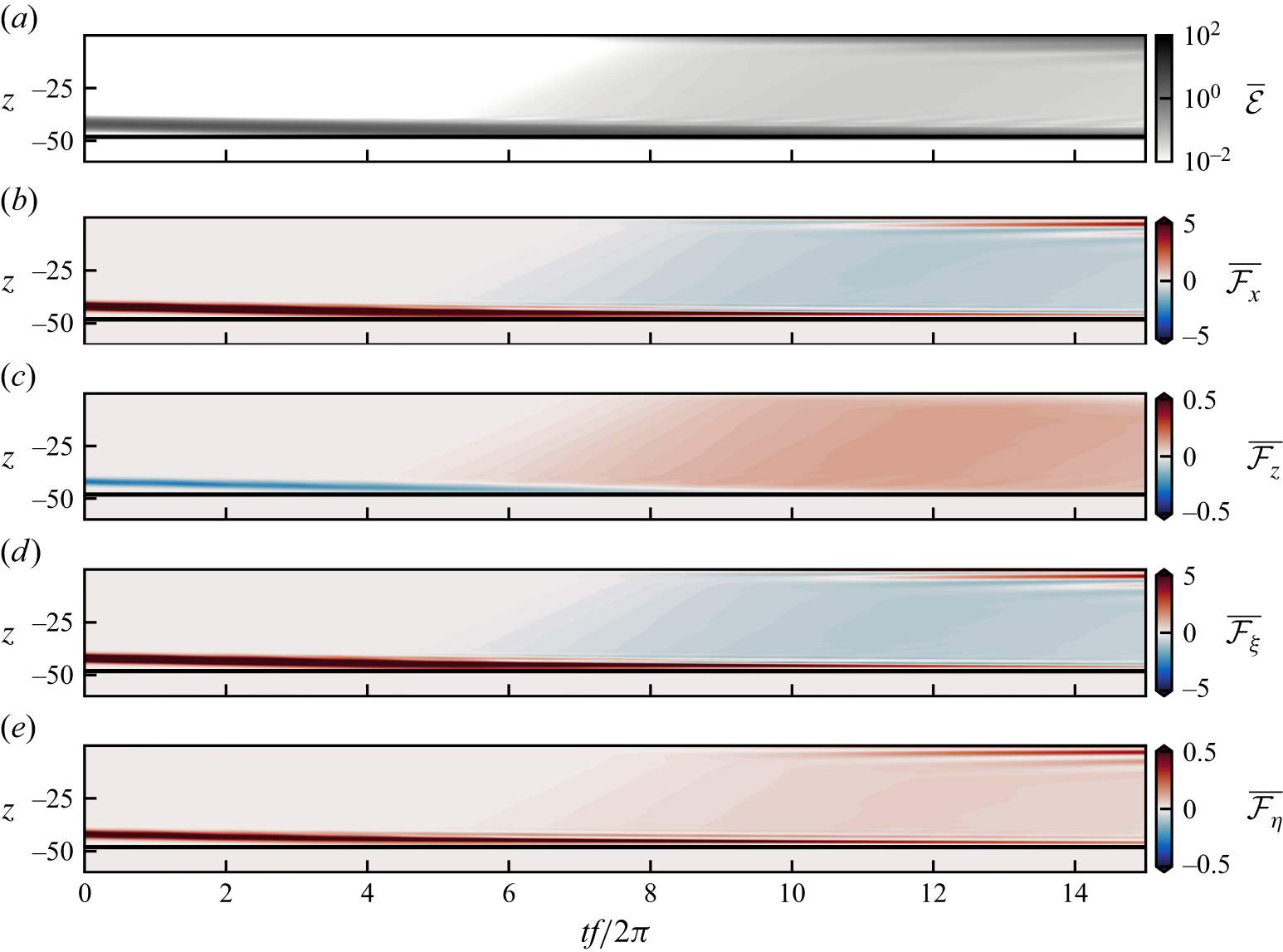


 Open access

