

Introduction
The article analyses the policy preferences of political actors in order to better understand collective policy formulation. In democratic systems, policy decisions rely on majorities formed through negotiations in decision-making processes. To create such majorities in line with their own preferences, actors have an incentive to convince others of their own policy preferences. Similar policy preferences are thus an outcome of strategic positioning in a power game to create majorities. Actors may position themselves given others’ preferences through the exchange of information (Leifeld and Schneider Reference Leifeld and Schneider2012) or mutual learning about the advantages and disadvantages of various policy options (Weible et al. Reference Weible, Pattison and Sabatier2010; Crona and Parker Reference Crona and John2012). Thereby actors create common interpretations or reasoning and influence the policy preferences of those they have been in contact with before.
Despite potential interdependencies between collective actors, there is a lack of research that conceives of policy preferences as an interdependent system. To address this research gap, we study mechanisms behind the formation of policy preferences of collective actors and take into account their interdependent choices. We analyse whether actors’ policy preferences are partly conditional on other actors’ choices, thereby forming a complex, interdependent system of preferences. More specifically, we ask: which joint properties lead actors to adopt similar policy preferences in the actor-instrument network?
The “actor-instrument network” refers to our conceptualisation of actors and their policy preferences as a two-mode network, where policy actors represent the first mode and policy preferences the second mode (for a similar approach see studies on the support/veto of legislative bills by members of parliament, see Zhang et al. Reference Zhang, Friend, Traud, Porter, Fowler and Mucha2008; Harward and Moffett Reference Harward and Moffett2010; Briatte Reference Briatte2016). We conceptualise policy preferences as support for, or rejection of, specific policy instruments. Policy instruments (e.g. bans, charges, information campaigns) are single means through which defined policy goals can be reached (Lasswell Reference Lasswell1958). Collective actors are organisations that participate in policy-making processes, including state-actors with formally assigned regulatory competences, and nonstate actors who contribute to the design or implementation of policies (Schneider Reference Schneider2014). A tie between an actor and a policy instrument indicates a preference (support or rejection) for that instrument by the actor. A complex two-mode actor-instrument network emerges as actors exhibit multiple preferences, and multiple actors can prefer the same policy instrument.
To better understand the mechanisms driving this interdependent system of preferences, we employ a model that specifically accounts for interdependencies of observations, called the exponential random graph model (ERGM) or p* model (Wasserman and Pattison Reference Wasserman and Pattison1996; Robins et al. Reference Robins, Pattison, Kalish and Lusher2007a, Reference Robins, Snijders, Wang, Handcock and Pattison2007b; Cranmer et al. Reference Cranmer, Leifeld, McClurg and Rolfe2017). The use of a network approach over dyadic logistic regression is necessary to model the dependencies between observations and avoid a resulting omitted variable bias because the actors possess mutual relevance and visibility in their instrument choices (Cranmer et al. Reference Cranmer, Leifeld, McClurg and Rolfe2017). While there exists a solid number of studies using ERGMs on one-mode data, fewer applications exist in the field of two-mode networks (but see Jasny Reference Jasny2012; Berardo Reference Berardo2014; Jasny and Lubell Reference Jasny and Mark2015). One contribution of this article is to introduce nonstandard endogenous model terms for the analysis of two-mode network data. Such methodological advances provide us with new tools to address the classic question of social theory about how behaviour (in our case policy preferences) is affected by social relations (Marsden Reference Marsden1981; Granovetter Reference Granovetter1985).
The theoretical contribution of this article consists of disentangling the different mechanisms that may lead actors to select the same policy. Bressers and O’Toole (Reference Bressers and O’Toole1998, Reference Bressers and O’Toole2005) highlight two important aspects of social settings that can influence the choice of instruments in the process of policy formulation. They term the first mechanism “cohesion”, which is about similarity in actors’ policy objectives that frame their choices for policy instruments (see also Jenkins-Smith et al. Reference Jenkins‐Smith, Silva, Gupta and Ripberger2014). For example, actors who have the goal of protecting the environment can be assumed to also share similar policy preferences. The second mechanism captures a relational dimension of policymaking and is called “interconnectedness”. Accordingly, actors who are linked by some sort of interaction in the policy process are more likely to develop similar policy preferences. “Interaction” is a generic term for any type of social relation, which in the case of policymaking involves, for example, information exchange, negotiations, or collaboration between policy actors. The distinction between similar objectives and interactions as two mechanisms influencing preference formation is a puzzling question, from a methodological and theoretical perspective.
Theory
The study of policymaking integrates different levels of analysis as one has to consider both the policy preferences on the individual actor level and their aggregate on the collective-level. How individual-level preferences are translated into collective decisions is a matter of scholarly debate. Actor-level approaches focus on micro-level explanations of policymaking. They claim that actors have intrinsic interests that guide their behaviour or policy preferences (Olson Reference Olson1965). Group-level approaches shift attention away from individual actors to networks of relationships and claim social foundations of policy preferences (Marsden Reference Marsden1981). A network approach is not only an aggregation of policy actors’ attributes, but it also takes into consideration actors’ interdependencies (Sandström and Carlsson Reference Sandström and Carlsson2008; Lubell et al. Reference Lubell, Scholz, Berardo and Robins2012). We explore the dialectical relationship between micro-level and meso-level foundations of preference formation by, first, considering actors’ joint attributes in the form of policy objectives and, second, actors’ interactions in the form of direct collaboration.
Interdependencies of policy preferences
Policymaking can be defined as the process during which actors work towards (a) an agreement upon political goals and (b) the selection of (appropriate) instruments to reach the defined goals (Landry and Varone Reference Landry and Varone2005; Howlett Reference Howlett2009). It is not solely the work of authorities or single actors, but policymaking happens in a complex and intertwined setting that includes various public and private collective entities who aim to transform their preferences into public policy through their participation in the policy-making process (Knill and Tosun Reference Knill and Tosun2012, 41). The increased interest in network-like constellations of policymaking comes along with the recognition that, in most cases, no organisation of government possesses sufficient authority, resources, and knowledge to enact and achieve policy intentions (Sabatier and Jenkins-Smith Reference Sabatier and Jenkins-Smith1993). Instead, policies require the concerted effort of multiple governmental and societal actors (Bressers et al. Reference Bressers, Huitema and Kuks1995, 4). In the study of environmental politics, the network approach is particularly relevant because pollution reduction requires the coordinated action of various sectors and levels across political boundaries. Thus, a networked policy subsystem is best approached through a network lens (Bressers et al. Reference Bressers, Huitema and Kuks1995, 7), which in our case involves a network of actors and their instrument preferences.
The network approach represents a shift of focus away from the policy instruments themselves (and their effects) to the actors participating in the process. Bressers and O’Toole (Reference Bressers and O’Toole1998) expect that network characteristics influence instrument selection (Majone Reference Majone1976). This argumentation is in line with the “logic of appropriateness” according to which actors (involved in policymaking) tend to reproduce existing features of the social system, that is, formal and informal power structures, roles, and institutions, through their policy choices (March and Olsen Reference March and Olsen1989; Sager Reference Sager2009). This logic can best be studied by conceptualising the policy process as a network, and by linking network features such as actors’ attribute similarity in terms of common objectives and their social relations to the choice of policy instruments. Bressers and O’Toole (Reference Bressers and O’Toole1998) employ the term “cohesion” to refer to similar policy objectives that bring actors together or divide them in policy negotiations. With “interconnectedness”, Bressers and O’Toole highlight the relational patterns linking state and nonstate actors, or elected authorities, and target groups. With strong similarity of objectives and high interconnectedness among network members, a wide range of policy instruments is possible as long as they keep the social system intact. Our contribution is to disentangle the two elements, policy objectives and interconnectedness, and to study their individual significance for policy preferences. Thereby, we seek to achieve a fine-grained understanding of the socio-political context in which policy instruments are selected.
Policy objectives
Key to understanding policymaking in general, and policy instrument selection in particular, is to consider the behaviour of those actors involved in formulating policies (Bressers and O’Toole Reference Bressers and O’Toole2005). A central element guiding political actors’ behaviour is their policy objectives, that is, the goals they seek to transform into public policy in order to achieve their desired societal changes. In their work, Bressers and O’Toole distinguish situations in which actors share objectives from those situations where actors exhibit conflictive objectives. In addition, they describe a third type of situation where actors’ objectives are not shared, but are nevertheless compatible and mutually reinforcing. In policy processes where diverse types of actors participate, it is likely to find a distribution of objectives − from conflictive over mutually reinforcing to shared. In order to describe the overall level of similarity of objectives among actors participating in decisionmaking, Bressers and O’Toole (Reference Bressers and O’Toole1998) employ the term “cohesion”. A high level of network cohesion describes a situation where network members, that is, those actors who participate in policymaking, share similar objectives. Cohesion, in turn, increases the probability of concerted instrument preferences.
Other branches of the literature have tried to explain in more detail what drives actors to share or diverge on policy objectives. One explanation is that actors involved in policymaking relate to the world through a set of perceptual filters that supports them in articulating policy objectives (Munro and Ditto Reference Munro and Ditto1997; Munro et al. Reference Munro, Ditto, Lockhart, Fagerlin, Gready and Peterson2002). These filters are termed “beliefs” in the terminology of the Advocacy Coalition Framework (Sabatier Reference Sabatier1999); other scholars refer to “mental models” (Pahl-Wostl Reference Pahl-Wostl2007) or “macroculture”, defined as norms and values shared across actors (Jones et al. Reference Jones, Hesterley and Borgatti1997; Robins et al. Reference Robins, Bates and Pattison2011). Such deeply rooted values or worldviews guide actors’ preferences in the more instrumental decisions of matching policy goals with the instruments to achieve those goals.
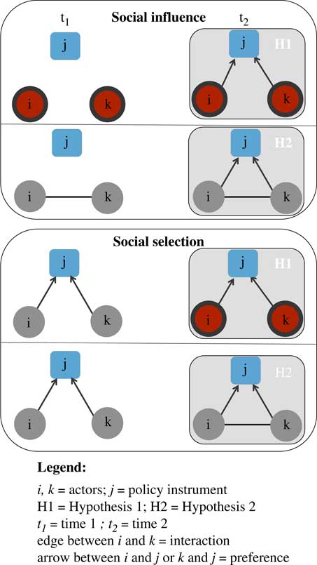
Based on these theoretical underpinnings, we expect that actors relate to a similar set of policy instruments because they exhibit shared or mutually reinforcing objectives. Such shared instrument preferences are irrespective of coordination between actors, but are rather a result of a similar attribute, that is, shared objectives in our case. Our hypothesis as depicted in Figure 1 reads as follows:
(H1) Policy objectives hypothesis: The more similar actors’ objectives are, the more likely they exhibit preferences for a similar set of policy instruments.
Schematic representation of Hypotheses 1 and 2. Note: Hypothesis 1 on common objectives: two actors (circles) with same objective (red/black circle attribute) prefer the same policy instrument (square). Hypothesis 2 on interconnectedness: two actors (circles) interact (tie between actors) and prefer the same policy instrument (square). In this article, we do not horizontally distinguish selection and influence mechanisms, but rather vertically between hypotheses.
Interconnectedness
Network scholars like Marsden (Reference Marsden1981) or Granovetter (Reference Granovetter1985, Reference Granovetter1992) drew attention to social dependencies, where actors’ attitudes are influenced by the attitudes of their social environment. In a similar vein, policy actors are elements of social structures and therefore do not only individualistically form instrument preferences, but rather socially. Interactions among network members are likely to socially influence actors’ attitudes, perceptions, behaviour, and policy preferences. From this perspective, not only do actors’ attributes (e.g., objectives) need to be understood in order to explain policy preferences, but also actors’ ties and their embeddedness in their social environment.
Particular to the political realm is that the structure of social relations reflects both formal hierarchy and informal bargaining processes. The logic of actors’ interactions is framed by macropolitical institutions, which define formal decision-making power, or participation mechanisms (Howlett and Ramesh Reference Howlett and Ramesh1995; Varone Reference Varone1998; Weible and Sabatier Reference Weible and Sabatier2005). However, the structure of policy networks does not only reflect the formal setup of the political (sub)system, but also informal aspects of policymaking. Informal aspects matter for network structures, because policy negotiations also involve actors without formal decision-making power participating in policy negotiations (Börzel Reference Börzel1998; Lubell et al. Reference Lubell, Scholz, Berardo and Robins2012). Actors without formal decision-making power, such as nonstate actors from the science community or interest groups, can participate, for example, in the preparliamentary phase of policy-making processes.
In the political realm, the structure of social relations matters to better understand how actors form their policy preferences. Actors create a social fabric in policy-making processes by initiating connections, for example, by collaborating. As such connections among actors entail crucial information about social structure, the literature elaborates on several indicators of interconnectedness: the degree of inclusion of actors in policy-making processes (Ingold et al. Reference Ingold, Varone and Stokman2013; Ingold Reference Ingold2014), the quality of ties between authorities and target groups (Linder and Peters Reference Linder and Peters1989; Varone Reference Varone1998) or the degree of conflict between opposing coalitions (Weible et al. Reference Weible, Pattison and Sabatier2010). Mutual relations among actors, such as collaboration or reciprocal information exchange, can create a common understanding of the policy-making process (Henry Reference Henry2011; Leifeld and Schneider Reference Leifeld and Schneider2012; Fischer and Sciarini Reference Fischer and Sciarini2016). Actors’ joint understanding of a situation, in turn, can lead to concerted policy preferences in a policy subsystem. Studies also demonstrate that interconnectedness establishes trust and social capital, which can enhance the creation of joint policy preferences (see Berardo and Scholz Reference Berardo and Scholz2010). In this line of thought, we hypothesise as depicted in Figure 1:
(H2) Interconnectedness hypothesis: Actors who interact with each other tend to exhibit a preference for similar policy instruments.
In summary, we observe the local topology (i.e. a structure of nodes and ties) of preference interdependencies as defined by three elements: actors’ attributes (objectives in our case), direct actor-actor interactions and actors’ policy instrument preferences. We analyse whether actors exhibit similar instrument preferences given, on the one hand, mutual policy objectives and, on the other, direct actor-actor interactions. In Hypothesis 1, we study whether the topology of preference interdependencies is paralleled by similar attributes of actors, namely their objectives, independently of coordination between actors. For example, two environmental organisations may both exhibit the objective to promote water protection and, therefore, support the instrument “effluent charge”. Despite their mutual objective, these actors do not necessarily coordinate their actions. Even without any transmission or exchange among actors, preference similarity exists. Similar policy preferences are consequently not a result of imitation or learning between actors in this mechanism, but rather an assortative mixing pattern (Newman Reference Newman2002), where environmental organisations simply tend to support certain instruments, such as effluent charges. In Hypothesis 2, on the other hand, we analyse situations where actors do interact directly and jointly support policy instruments.
Our hypotheses are compatible with two causal mechanisms: social influence and social selection, which are generally confounded in observational studies of social networks (Shalizi and Thomas Reference Shalizi and Thomas2011). Social influence (also known as diffusion or contagion; see also Gilardi Reference Gilardi2016; Lindstädt et al. Reference Lindstäd, Vander Wielen and Green2017) posits that actors share attributes (Hypothesis 1) or collaborate (Hypothesis 2) first and then align their policy preferences in the two-mode network (see temporal pattern t 1 and t 2 in Figure 1). Selection (also known as homophily)Footnote 1 posits that actors have congruent policy instrument preferences in the two-mode network first and develop shared attributes (Hypothesis 1) or collaboration ties (Hypothesis 2) as a consequence. Malang et al. (Reference Malang, Brandenberger and Leifeld2017) demonstrate using a causal inference approach with temporal permutations that a causal identification strategy in this situation is only feasible if the timing of policy instrument preferences is measurable in a temporally fine-grained way on a nearly continuous time scale, which is next to impossible to implement for organisations’ policy instrument preferences. In this article, we do not distinguish between social influence and selection effects in networks (as e.g. in Malang et al. Reference Malang, Brandenberger and Leifeld2017). We rather describe instrument preferences as an interdependent system given attribute similarity (common objectives) or direct ties (interactions) in order to discriminate between the specific patterns in the actor-instrument networks as shown by Hypotheses 1 and 2 in Figure 1. In Figure 1, we focus on the dark shaded actor-instrument networks, which either describe Hypotheses 1 or 2, but we do not incorporate the temporal dimension between t 1 and t 2, that is, between left and right panels of Figure 1.
Case and data
Although our research question regarding the formation of policy preferences is relevant across policy domains, our study concentrates on environmental policy. The interplay between different types of actors is particularly relevant in environmental governance where diverse claims regarding the use and the protection of natural resources have to be balanced in policymaking. The integration of various stakeholders into environmental decisionmaking is often not a normative claim anymore, but an observable reality, namely through the establishment of collaborative governance structures (Lubell and Fulton Reference Lubell and Fulton2007; Bodin and Crona Reference Bodin and Crona2009; Newig and Fritsch Reference Newig and Fritsch2009; Bodin and Prell Reference Bodin and Prell2011; Ostrom et al. Reference Ostrom, Cox and Schlager2014; Fischer and Leifeld Reference Fischer and Leifeld2015). Environmental policy is therefore particularly well suited to analyse interplays between policy actors and the degree to which their exchanges affect the formulation of policy preferences.
More specifically, we take the case of water protection policy in Switzerland where there is growing policy attention to what are called “micropollutants” or “emerging pollutants”, a large quantity of diverse chemicals that have only recently been detected and deemed a concern in water bodies due to improvements in analytical measurement technology (Schwarzenbach et al. Reference Schwarzenbach, Escher, Fenner, Hofstetter, Johnson, Von Gunten and Wehrli2006). Sources of such micropollution include, for example, the use of pharmaceuticals, personal care products, detergents, biocides or plant protection products (Hollender et al. Reference Hollender, Singer and McArdell2008). Due to the large number of substances, sources and entry-paths into the aquatic environment, it is a complex task to develop a pertinent policy response to the issue of micropollutants in water bodies and to choose among the many policy alternatives that exist. It is an ideal case to study policy preferences as the issue is rather new on the political agenda, and different actors involved in policymaking debate about a large variety of instruments that could potentially be introduced (Metz and Ingold Reference Metz and Ingold2014).
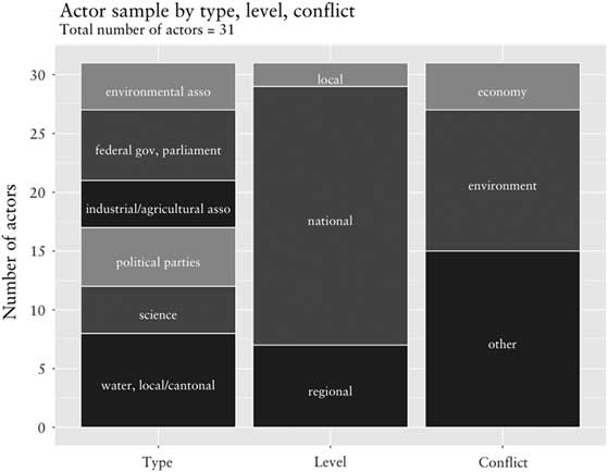
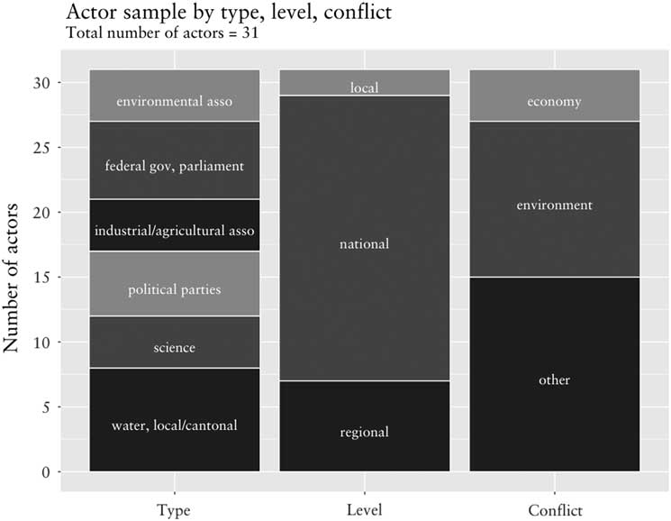
Switzerland is a pioneer in this emerging policy domain, since the issue entered the political agenda in the early 2000s and concrete measures have been debated since then. The present study examines the amendment process of the Swiss Waters Protection Act and Ordinance that took place between 2007 and 2014, during which Swiss policy actors negotiated how to best address micropollutants from point sources of pollution, that is, from household wastewaters. From April to July 2013, we surveyed state and nonstate collective actors, who participated and have a stake in this policy process on micropollutants, including governmental bodies, science, political parties, water, environmental and economic associations. We surveyed policy actors when they (a) participated at least twice in the process of amending the Waters Protection Act and Ordinance (decisional approach), or (b) hold formal regulatory competences in the domain of emerging water pollutants (positional approach, or (c) were considered important by knowledgeable experts in the field (reputational approach) (Laumann et al. Reference Laumann, Marsden and Prensky1983; Knoke Reference Knoke1994). In total, 32 actors (or 31 as one actor exhibits missing data on the objectives variable) replied to the relevant survey questions (see Figure 2 for the precise composition of the actor sample and Online Appendix 1 for the list of actors).
Actor sample by type, level and conflict, n=31.
We surveyed actors’ preferences about 15 policy instruments for the reduction of micropollutants on a four-point Likert scale, where respondents could indicate from 1 to 4 whether they strongly disagreed (1), disagreed somewhat (2), agreed somewhat (3) or strongly agreed (4) with the policy instrument. Table 1 provides an overview about the 15 different regulatory, economic and voluntary policy tools that were surveyed. We generated the list of instruments based on an inventory of instruments in water protection (Metz and Ingold Reference Metz and Ingold2014).
Overview about surveyed instrument preferences

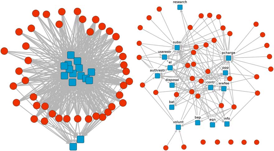
Figure 3 shows the two-mode networks of actors (circles) and their preferences towards the surveyed policy instruments (squares). The data reveals, in the overwhelming majority of cases, positive (agree somewhat) to very positive (strongly agree) results (see left part of Figure 3). Survey respondents agree with many different policy options in principle (see left part of Figure 3), while they have very specific ideas about what types of instruments they reject. The interesting variation thus occurs where respondents indicate that they disagree somewhat or disagree strongly with a policy instrument (see right part of Figure 3). This observation aligns with research focusing on opposition against policy instruments (see, e.g. Kammermann and Dermont Reference Kammermann and Dermont2018). When actors oppose a specific policy instrument (mix), they can potentially block the entire decision-making process. As opposition is crucial to the choice of policy instruments (Keohane et al. Reference Keohane, Revesz and Stavins1998), we focus on policy preferences in the form of rejection rather than agreement. Rejection and support can be modelled interchangeably here because there is no neutral category such that “not rejecting” is equivalent to supporting.
Two-mode network of policy instrument preferences. Note: Support network (“agree somewhat” or “strongly agree”) on the left; rejection network (“disagree somewhat” or “strongly disagree”) on the right. Circles=actors, squares=policy instruments, ties=preferences in the form of support or rejection.
For our independent variables, the survey further included several questions capturing actors’ objectives (Hypothesis 1) and their interconnectedness (Hypothesis 2). In water protection, actors can prioritise addressing the sources of pollution or the “end of the pipe”. We elicited actors’ objectives by asking respondents for their level of agreement, ranging from strongly agree (coded as 4) to strongly disagree (coded as 1), with the five following statements:
∙ Measures should address the sources of pollution.
∙ Measures should be end-of-pipe.
∙ Precautionary measures should be taken to reduce potential risks for humans and the environment (precautionary principle).
∙ It is reasonable to wait with policy measures until the impact of micropollutants is fully understood (risk-based principle).
∙ Policy measures should aim at completely eliminating micropollutants in waters.
Source-directed policy objectives reflect actors’ goal to prevent the release of pollution into water in order to reduce human impact on the environment. End-of-pipe objectives, by contrast, focus on eliminating pollutants after their use and release into water and echo actors’ priority in maintaining current consumption and production patterns. The precautionary principle stands for the goal to adopt policy measures despite existing uncertainties about adverse impacts of micropollutants on humans or the environment. The risk-based principle, by contrast, is in line with the objective that policy action is only needed where risks have been proven. Finally, actors’ objectives could diverge with regard to the level of pollution permitted (or admitted to be unavoidable) in water.
We further collected responses on actors’ policy agenda priorities. Respondents were asked to rate the reduction of micropollutants as a higher priority, equal, or lower priority compared to 10 other water policy issues, that is, (1) ecological status of water bodies, (2) classic “macropollution” such as nutrients/fertilisers, (3) industrial emissions, (4) wastewater treatment, (5) water levels, (6) ground water, (7) drinking water, (8) hydropower, (9) flood protection, (10) water monitoring.
Moreover, with the information about respondents’ actor types (federal-state, political party, regional/water/local, environmental, industrial/agricultural, science), we classified them into two groups. The first group consists of water and green organisations, and the second one of industrial and agricultural organisations.
While the data described above serve as different proxies for policy objectives, the following data capture interconnectedness. We surveyed respondents’ interconnectedness by asking them with whom their organisation closely collaborated during the Swiss policy process on micropollutants between 2007 and 2013. Respondents could check all their collaborators from a list of actors that we previously identified by applying the positional, decisional and reputational approach; respondents could add missing actors to the list. Close collaboration was defined as discussing new findings, developing policy options, exchanging positions, evaluating alternatives. Not only interactions with Swiss actors may be relevant, but also with international actors, for example, during transboundary water basin meetings. We therefore asked respondents to report their memberships in international water basin organisations and then coded their comemberships.
Methodology
We estimate a bipartite (=two-mode) ERGM (Wasserman and Pattison Reference Wasserman and Pattison1996) to explain the policy instrument preferences of actors. A two-mode network or bipartite graph is a network with two separate types of nodes that displays the connections (also known as ties) between the two node types. In our case, 32 policy actors comprise the first node type (or mode), and 15 policy instruments comprise the second mode. Ties in this network are the instrument choices actors make. Within-mode ties are not possible on the dependent variable because a bipartite graph is mathematically defined by between-mode ties. We chose a bipartite network model because the explanandum is the portfolios of instrument preferences the actors collectively hold, not the relations between actors or between preferences. For methodological details on bipartite ERGMs, see Wang et al. (Reference Wang, Sharpe, Robins and Pattison2009). For applications to policy networks, see Berardo (Reference Berardo2014) and Jasny and Lubell (Reference Jasny and Mark2015). To accommodate the bipartite network structure, the normalising constant of the ERGM was adjusted accordingly by the software we employed for estimation, the R package ergm (Hunter et al. Reference Hunter, Handcock, Butts, Goodreau and Morris2008). Goodness of fit was assessed using the xergm package (Leifeld et al. Reference Leifeld, Cranmer and Desmarais2018), and regression tables were created using the texreg package (Leifeld Reference Leifeld2013).
The network we model is policy instrument rejection, as depicted on the right in Figure 3, while the reference group (the nonties) contains all agreement ties depicted on the left in Figure 3. By modelling the sparser relation (rejection) instead of the denser complementary relation (agreement), we count fewer instances of endogenous network statistics such as two-stars and shared partners. This makes the model more easily identifiable without having to redefine the endogenous network statistics for the ERGM. However, since agreement ties are treated as the baseline in the model, this means only a conceptual, but not a substantive change.
The ERGM is a parametric model of the configuration of ties in a given network. Unlike a logistic regression model, the ERGM permits unbiased estimation of parameters for endogenous model terms that specify dependencies between observations (Cranmer et al. Reference Cranmer, Leifeld, McClurg and Rolfe2017). It is important here to take into consideration that the profile of policy instrument preferences of one actor may depend, in part, on the preferences of another actor. We capture these dependencies by constructing respective model terms.
The probability density function of the ERGM is given by
 $$P\left( {N,\,{\bf \btheta }} \right){\equals}{{\exp \left\{ {{\bf \btheta }^{{\rm T}} {\bf h}\left( N \right)} \right\}} \over {\sum_{N^{{\rm {\asterisk}}} \in{\cal N}} \exp \left\{ {{\bf \btheta }^{{\rm T}} {\bf h}\left( {N^{{\rm {\asterisk}}} } \right)} \right\}}}$$
where the θ vector denotes the parameters of the model terms, the h vector contains the model terms and the denominator represents the same sum of weighted statistics as the numerator, over all the network configurations one could have observed (Cranmer et al. Reference Cranmer, Leifeld, McClurg and Rolfe2017). In the analysis, our task is to specify the exogenous and endogenous effects, or h statistics, that contribute to the topology, or structure, of the network.
These network statistics are conveniently specified as sums of subgraph products (see Cranmer et al. Reference Cranmer, Leifeld, McClurg and Rolfe2017 for details). For example, the number of two-stars found in the network can be defined as the sum of the product of local configurations N ij and N kj , where N ij equals 1 if there is a tie from actor i to instrument j and 0 otherwise, and N kj equals 1 if there is a tie from actor k to instrument j and 0 otherwise. Estimation was carried out through Markov Chain Monte Carlo (MCMC) Maximum Likelihood Estimation (Hunter et al. Reference Hunter, Handcock, Butts, Goodreau and Morris2008). Online Appendix 2 contains details about the estimation as well as robustness checks and alternative model specifications.
Model terms
We first introduce the model terms for our independent variables, then for the controls. Our two main variables, policy objectives and interconnectedness, can be operationalised in different ways. For the purpose of clarity, we therefore distinguish three versions of Hypotheses 1 and 2, which in fact capture the same theoretical concept with slight nuances regarding measurement.
These model terms are conceptualised as bipartite homophily terms of the following form:
 $$h_{{{\rm homophily}}} {\equals}\mathop \sum\limits_i \mathop \sum\limits_j \mathop \sum\limits_{k\,\ne\,i} \left( {N_{{ij}} N_{{kj}} f\left( {i, k, X} \right)} \right)$$
where f(i,k,X) is some function of an exogenous actor covariate, which is stored in a square m×m matrix X, and actor indices i and k. We call this a “homophily” term because this model term tests whether a common property, such as a shared attribute or a collaboration tie, contributes to the probability that both actors i and k choose to have ties to the same instrument j.
More technically, this term counts instances of open triangles where both actors i and k are jointly connected to the same policy instrument j through rejection ties, weighted by some shared or joint characteristic as expressed through a function of the exogenous covariate. For example, this model term could be used to count how often two actors who collaborate or who have some shared property jointly reject policy instruments. In other words, this statistic captures the tendency of actors to coreject or cosupport policy instrument preferences when they share certain characteristics, which will be detailed below.
Hypothesis 1a: policy objectives
The first measure of attribute similarity is operationalised through our data on policy objectives. Those objectives frame the more specific instrument preferences held by actors (Bressers and O’Toole Reference Bressers and O’Toole1998; Sabatier Reference Sabatier1999). Let X be a 32×5 matrix with the row actors’ policy objectives on a Likert scale from 1 to 4.
The similarity in environmental policy objectives between actors i and k is defined as the inverse Euclidean distance (i.e. proximity) between rows in the policy objective matrix:
 $$f_{{{\rm objectives}}} \left( {i, k, X} \right){\equals}{1 \over {\sqrt {\sum_l \left( {X_{{il}} {\minus}X_{{kl}} } \right)^{2} } }}$$
where l is the column index of the policy objective matrix and points to a specific objective. In other words, the h homophily model term with f objectives(i,k,X) captures the tendency of two actors i and k with shared objectives to coreject the same policy instruments.
Hypothesis 1b (policy objectives): agenda priorities
Actors differ in terms of the importance they ascribe to the micropollution problem relative to other issues related to water, such as the issues of flood prevention or hydropower. We identified ten issues including (1) ecological status of water bodies, (2) classic “macropollution” such as nutrients/fertilisers, (3) industrial emissions, (4) wastewater treatment, (5) water levels, (6) ground water, (7) drinking water, (8) hydropower, (9) flood protection, (10) water monitoring. We then measured actors’ judgements of each issue’s importance relative to micropollution (1=more important than micropollution; 0=equally important; −1=less important). Each actor has a priority profile over these issues, with one of these three objectives for each issue. This yields a 32×10 issue prioritisation (or “agenda”) matrix A.
The question we would like to answer with regard to issue prioritisation is whether two actors who evaluate the issue of micropollutants as similarly important compared to other water policy issues tend to prefer similar policy instruments. This is accomplished by counting the number of two-stars centred on instrument j weighted by the similarity of priority profiles of actors i and k involved in the k-star. This corresponds to the following function, which is identical to the previous f objectives(i,k,X) function with a new covariate matrix A for the actors’ issue prioritisation or agendas:
 $$f_{{{\rm issue}{\minus}{\rm prioritization}}} \left( {i,\,k,\,A} \right){\equals}{1 \over {\sqrt {\sum_l \left( {A_{{il}} {\minus}A_{{kl}} } \right)^{2} } }}$$
In other words, we compute the inverse of the Euclidean distance of any two row actors in terms of their issue prioritisations and weight any actor-instrument-actor two-path in the rejection graph by the similarity term.
Hypothesis 1c (policy objectives): conflict
We also test whether material interest conflicts lead to diverging evaluations of policy instruments. We accomplish this by defining an explicit conflict line that we expect to be present in the data: if actor i is a water association or environmental association and actor k is an industrial or agricultural association, we expect conflicting opinions on how micropollution should be regulated. To do this, we insert the following function into the bipartite homophily model term defined above. The term captures the tendency of the network to have actor pairs with jointly present rejection ties to an instrument and who have conflicting organisational types:
 $$\eqalignno{ & f_{{{\rm org}{\minus}{\rm type}{\minus}{\rm conflict}}} \left( {i, k, x} \right){\equals}\left[ {x_{i} {\equals}{\rm industry}\,/\,{\rm agriculture}} \right] \cdot \left[ {x_{k} {\equals}{\rm environment}\,/\,{\rm water}} \right] \cr & {\plus}\left[ {x_{i} {\equals}{\rm environment}\,/\,{\rm water}} \right] \cdot \left[ {x_{k} {\equals}{\rm industry}\,/\,{\rm agriculture}} \right] $$
where x denotes a vector of categorical actor types and square brackets are an indicator function that returns 1 if true and 0 otherwise.
We expect a negative coefficient for this model term as the presence of a conflicting actor type configuration should lead to less corejection of instruments than in nonconflicting actor type configurations.
The conflict hypothesis is strongly related to Hypothesis 1a on congruence of objectives. But rather than measuring congruence of objectives or conflict at a more abstract level of values or norms, Hypothesis 1c evaluates how strongly the similarity of objectives matters in terms of the functional roles actors take.
Hypotheses 2a (interconnectedness): collaboration
Let C be a 32×32 binary matrix indicating collaboration between actors i and k. Then including
 $$f_{{{\rm collaboration}}} \left( {i,k,C} \right){\equals}C_{{ik}} $$
in a bipartite homophily model term measures the tendency of actors to reject instruments that other actors with whom they maintain collaboration ties also reject. In other words, this term tests whether actors’ interconnectedness, operationalised through the maintenance of collaboration ties, is associated with similar policy preferences.
The article is about a bipartite, or two-mode, network of actors and instrument preferences as defined in the homophily statistic above. Here, we employ a one-mode network matrix C in the construction of the bipartite model term. Theoretically, this tests whether one-mode collaborations are associated with similar policy instrument preferences in the two-mode network.
Hypothesis 2b (interconnectedness): structural similarity in the collaboration network
If C denotes the 32×32 binary collaboration network matrix, a structural similarity matrix can be computed as follows:
 $$Z{\,\equals\,}CC^{{\rm T}} $$
This matrix denotes how many collaboration partners two actors have in common. It is a measure of similarity in collaboration interactions, and more specifically, in terms of the structural position in the network. Structural similarity in the collaboration network tests whether actors with an overlap in their collaboration profiles are more likely than chance would predict to coreject the same policy instruments:
 $$f_{{{\rm collaboration{\minus}structsim}}} \left( {i,k,Z} \right){\,\equals\,}Z_{{ik}} $$
This is a valuable alternative conceptualisation of interconnectedness because interconnectedness may not only pan out directly through collaboration ties, but may be equally plausible through joint neighbourhoods in the collaboration network. Joint exposure to common collaboration partners may spark the adoption of similar policy instrument preferences (or vice versa).
Hypothesis 2c (interconnectedness): comembership in water basin organisations
Not only direct and indirect collaboration, but also mutual memberships in international water basin organisations can be an indicator of regular contact and interactions between two actors. When actors are members of the same water basin organisation or platform, this significantly increases their chance of regularly exchanging information on policy preferences (Leifeld and Schneider Reference Leifeld and Schneider2012; Fischer and Leifeld Reference Fischer and Leifeld2015). Let B be a 32×2 binary matrix indicating collaboration between actors i and international collaboration partners l. Then we are interested in whether the cooccurrence network BB T exerts any influence on the policy instrument preferences of actors. In other words, is an actor likely to reject (support) an instrument if there are many other actors who also reject (support) the same instrument with whom the focal actor shares international collaboration partners? This tendency is captured by inserting the following quantity into the bipartite homophily model term:
 $$f_{{water{\minus}body}} \left( {i,{\rm }k,{\rm }B} \right){\equals}\mathop \sum\limits_l B_{{il}} B_{{kl}} $$
Endogenous control: edges
The edges term counts the number of edges in the two-mode network. This can be interpreted like a constant in a generalised linear model and serves as a baseline for the probability of edges in any dyad in the network:
 $$h_{{{\rm edges}}} {\equals}\mathop \sum\limits_i \mathop \sum\limits_j N_{{ij}} $$
Including the edges term is necessary in any ERGM, because it controls for the baseline edge probability, in this case the general rate of policy instrument rejection (like the offset α in a linear regression model).
Endogenous control: actor degree 0
Figure 3 (right panel) displays a number of actors that do not reject any policy instruments at all. This is an endogenous property of the network that distinguishes it from a random graph with the same number of nodes and edges. Therefore, we need to control for the number of actors with degree 0 (“isolates”) to avoid omitted variable bias due to an incomplete specification of the endogenous part of the data-generating process:
 $$h_{{{\rm isolates}}} {\equals}\mathop \sum\limits_i \left[ {\mathop \sum\limits_j N_{{ij}} {\equals}0} \right]$$
Endogenous control: instrument two-stars
Some policy instruments receive many rejection ties while others are almost universally accepted. A two-star effect centred on the second mode (policy instruments) tests whether one rejection of an instrument is related to another rejection of the same instrument or, in other words, whether there is a popularity effect at work in which rejections tend to cluster within instruments. This may be the case if some instruments are universally considered poor solutions, for example. The two-star effect is defined as follows:
 $$h_{{{\rm instrument}{\minus}{\rm popularity}}} {\equals}\mathop \sum\limits_i \mathop \sum\limits_j \mathop \sum\limits_{k\,\ne\,i} N_{{ij}} N_{{kj}} $$
Including this term as a control variable is also important to distinguish the bipartite homophily effects defined above from the mere popularity of certain policy instruments.
Endogenous control: geometrically weighted nonedgewise shared partners (GWNSP)
Finally, we control for GWNSP, a typical dependency term for capturing clustering in two-mode networks. This model term computes the tendency of the network to have open two-paths, and it discounts higher numbers of two-paths between the same nodes. A two-path can exist between actors (via one or more instruments) or between two instruments (via one or more actors). GWNSP counts how many such two-paths exist between any given within-mode dyad, computes the aggregated distribution over the whole network, and sums up the counts in a geometrically weighted way by down-weighting higher numbers of shared partners geometrically (here: with an α parameter of 2.0). The definition of GWNSP (following the exposition of Hunter Reference Hunter2007) is
 $$h_{{{\rm GWNSP}}} \left( \alpha \right){\equals}e^{\alpha } \mathop \sum\limits_{i{\equals}1}^{n{\minus}2} \left\{ {1{\minus}\left( {1{\minus}e^{{{\minus}\alpha }} } \right)^{i} } \right\}EP_{i} \left( N \right)$$
where α is the geometric decay parameter (chosen inductively by model fit), and EP i (N) is the number of dyads within the same mode that have exactly i shared partners. This weighted count effectively controls for clustering in the network in the sense that actors share multiple corejections and instruments are corejected by multiple actors. Omitting this endogenous dependency would yield biased estimates of the main hypotheses because homophily terms may be statistically conflated with the general tendency for corejection of instruments if not modelled separately.
Exogenous control variable: degree centrality in the collaboration network
The effects related to collaboration between actors can only be interpreted in a valid way if we control for the number of collaboration ties actors have in the first place (i.e. their activity). Therefore we also include the number of ties, or degree, of any actor:
 $$h_{{{\rm collaboration}{\minus}{\rm degree}}} {\equals}\mathop \sum\limits_i \mathop \sum\limits_j \left( {N_{{ij}} \mathop \sum\limits_k X_{{ik}} } \right)$$
Exogenous control: nonadjacent competence level
Assume g is a vector of ordinal-scaled competence levels of policy actors from 1 (national level) to 3 (local level).
This term tests whether actors at nonadjacent and nonidentical levels (i.e. national and local) have less congruent policy instrument preferences:
 $$f_{{complevel{\minus}nonadjacent}} \left( {i,k,g} \right){\equals}\left[ {\,\mid\,g_{i} {\minus}g_{k} \,\mid\gt\,1} \right]$$
The square brackets denote an indicator function, which returns 1 if the term inside the parentheses is true and 0 otherwise. In this case, the function returns 1 if the absolute distance between the competence levels is larger than 1, that is, if one actor has a competence level of 1 (=national level) and the other one 3 (=local level). The function is inserted into a bipartite homophily model term defined above.
It is plausible that actors at the same level develop shared approaches to dealing with a problem. It is still somewhat plausible that actors of adjacent levels, that is, local and regional or regional and national actors, influence each other’s instrument choices somewhat, respectively. Therefore we control whether a spillover of instrument preferences across nonadjacent levels is implausible in order to yield a clean test for the other hypotheses.
Results
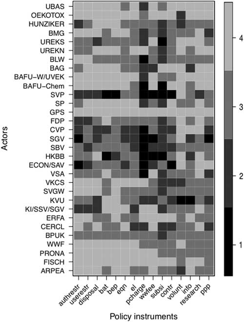
Figure 4 illustrates which types of policy instruments received particularly high rejection rates (squares in black and dark grey coded as 1 and 2) and support (squares in light grey coded as 3 and 4). There are high levels of support with most types of policy interventions, which further illustrates that opposition towards policy instruments is the crucial point of negotiation rather than the support of instruments. Economic instruments (product charges, wastewater fees, subsidies) enjoy the highest rejection rates, while most regulatory and voluntary instruments are far less controversial.
Instrument preferences for 15 policy instruments, from most coercive instruments on the left to least coercive instruments on the right (for an explanation of the surveyed policy instruments, see Table 1). Note: squares in black and dark grey coded as 1 and 2=rejection, squares in light grey coded as 3 and 4=support; 31 surveyed actors are ordered by conflict line. Bottom=advocates of water protection (including: ARPEA to WWF=environmental associations, BPUK to VSA=water and local/cantonal), middle=advocates of economy (including: ECON/SAV to SGV=industry/agricultural associations, CVP and SVP=conservative parties), top=other (including: FDP to SP=political parties, BAFU-Chem to UREKS=federal government and parliament, BMG to UBAS=science).

The actors in Figure 4 are ordered according to conflict lines. Actors who advocate water protection (from ARPEA to VSA) appearing in the bottom part of Figure 4 tend to support a variety of policy instruments with one exception: KVU, the Cantonal Offices for Environmental Protection, rejects voluntary instruments and information campaigns as too “soft”. By contrast, actors who represent industrial and agricultural interests (from ECON/SAV to SGV and conservative parties such as SVP or CVP) reject a greater variety of policy instruments, in particular economic ones such as charges on products containing harmful substances or a wastewater fee.
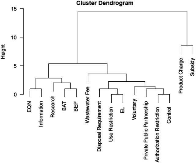
We previously illustrated the distribution of instrument preferences and turn now, in Figure 5, to the patterns behind interdependencies of policy preferences. As the opposition towards one policy instrument may logically preclude the opposition for another, there may be a strong tendency for policy preferences to cluster. Figure 5 shows combinations of instrument preferences in form of corejection as computed by a hierarchical cluster analysis. There is no clear clustering pattern, apart from product charges and subsidies that actors tend to coreject in common. Results indicate that preference formation is not a function of the popularity of certain instruments, but rather the result of more complex social processes.
Preference profiles of actors’ opposition (strongly disagree and disagree somewhat) towards 15 policy instruments, number of actors=31. Note: Dendrogram based on an agglomerative hierarchical cluster analysis with complete linkage of Euclidean distances of the instrument×actor matrix.
In order to understand the structure of preference interdependencies given common objectives or direct interactions, we estimated two models. The first model includes all hypotheses except for Hypothesis 1a (“policy objectives”). The second model includes all model terms. The reason for this is that to include Hypothesis 1a, it is necessary to drop one of the 32 actors because one actor exhibits missing data on this variable, and ERGMs can only be estimated if there are no missing data. The predictive (within-sample) performance, as indicated by the area under the receiver-operating characteristic curve (AUC-ROC) and the area under the precision-recall curve (AUC-PR), is identical in the two models, as are the substantive results.
The findings in Table 2 show that there are interdependencies between actors’ policy preferences. We observe significant patterns for actors sharing multiple policy preferences (a positive effect for nonedgewise shared partners), meaning that actors tend to reject multiple policy instruments in common, rather than just one. Together with the negative two-stars coefficient, the results indicate that actors do not reject instruments independently of the preferences of other actors, but they rather tend to reject several policy instruments jointly. If an instrument is rejected by one actor, it tends to be rejected by other actors, too, but only if actors agree on rejecting several instruments jointly. There is thus a considerable social dimension in developing policy instrument preferences.
Results for the bipartite exponential random graph model with standard errors in parentheses

Note: AUC=area under the curve.
***p<0.001, **p<0.01, *p<0.05.
In order to explain this complex, interdependent system of preferences we analysed actors’ similarities in policy objectives. Our first operationalisation of Hypothesis 1 on policy objectives does not yield any significant results. The same holds true for our second operationalisation capturing agenda priorities that actors attribute to the issue of micropollutants. These results indicate that actors do not tend to align their preferences with others who are similar in terms of policy objectives or agenda priorities. By contrast, ideological conflict lines between water or environmental organisations, on the one hand, and industrial or agricultural organisations, on the other, systematically shape the topology of instrument preferences. In line with our expectations, actors who are divided by a conflict line are less likely to exhibit interdependent policy preferences. A conflict line between actors advocating the use of water resources and actors advocating the protection of them reduces their odds of corejecting policy instruments. Overall, we find mixed evidence for the policy objectives hypothesis. A conflict line divides actors along environmental and economic objectives. This conflict line is the only significant factor operationalising Hypothesis 1 that is associated with the corejection of policy instruments.
We find significant results for actors’ interconnectedness in the form of collaboration ties. Whether actors collaborate with each other is significantly associated with their instrument preferences. In our case of water protection policy, actors collaborated, for example, within working groups that the Federal Office for the Environment initiated in the framework of its “Strategy Micropoll” as of 2007. Those groups were composed of diverse actors including cantons, operators of treatment plants, drinking water associations, science and industry. Within those groups, actors discussed the water issue at hand and exchanged their positions on policy options thereby creating common interpretations of the problem and solutions. The policy process provided further opportunities for collaboration during the elaboration of the draft legal revision, consultations or parliamentary debates. In sum, actors who participated in the policy process had numerous occasions to collaborate and develop shared instrument preferences.
We do not only expect that collaboration induces shared instrument preferences (Figure 1, social influence, lower panel), but also that shared prior instrument preferences may lead to collaboration (Figure 1, social selection, lower panel). An actor is more likely to reject a policy instrument if the actor collaborates with a number of actors who also reject the same instrument, and two actors likely collaborate if they have shared policy instrument preferences. Our results further corroborate the hypothesis according to which collaboration and instrument preferences interrelate in policy networks (Zafonte and Sabatier Reference Zafonte and Sabatier1998; Fischer and Sciarini Reference Fischer and Sciarini2016).
We also tested whether actors who occupy similar positions in the collaboration network – that is, have the same shared contacts – (structural similarity) corejected the same instruments, but this is not the case. Indirect influence through shared collaborators does not play a role for the development of policy instrument preferences. Moreover, joint memberships in water basin organisations do not stimulate deliberation to the extent that shared memberships in these forums lead to shared policy instrument preferences, while controlling for actual collaboration between actors. Overall, there is support for the interconnectedness hypothesis, but only through direct collaboration, not through shared contacts or joint forum participation.
We also tested the three mechanisms within each hypothesis separately (see Models 2b–2f in Online Appendix 2) to avoid statistical problems with multicollinearity among predictors of the same theoretical category. Moreover, we tested one group of hypotheses at a time in a separate model specification to rule out multicollinearity between Hypotheses 1 and 2 (Model 2g in Online Appendix 2). These modifications did not change the conclusions substantively, which indicates that these are indeed complementary hypotheses rather than substitutes.
Conceptualising policy instrument preferences as a two-mode, rather than one-mode, network helps disentangling policy objectives from interconnectedness because modelling a one-mode projection of instrument preference similarity among actors would likely remove variation at the level of instruments that generates differences between policy objectives and interconnectedness. This more thorough approach therefore suggests that elements from both actors’ objectives and their interconnectedness play a role in the interdependent structure of policy instrument choices among actors.
Regarding the exogenous control variables, results are significant for the activity (i.e. centrality) of actors in the collaboration network. Well-connected actors are less likely than expected by chance to coreject policy instruments. There is no compelling evidence for shared instrument preferences when actors are geographically close to each other. Similarly to collaboration, this control variable models the proximity between actors. Geographical proximity, however, does not considerably impact actors’ interdependent choices. Results for competence levels (nonadjacent refers to local versus national level) are not significant. Actors of adjacent levels do not tend to prefer similar policy instruments. The endogenous control variable “actor degree: 0” indicates that there are more isolates in the actor-instrument network, that is, actors who do not reject any instrument, than expected by chance in networks of this size.
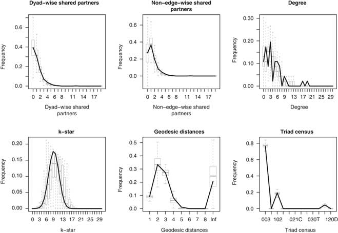
Figure 6 displays endogenous goodness of fit diagnostics for our Model 2, which illustrate that we capture the endogenous properties of the network very well. The six panels show common auxiliary network statistics in the observed network (the black lines) and in 500 simulations from the estimated model (the grey boxplots). As the boxplot medians are usually very close to the observed statistics, we seem to have properly captured network dependence.
Endogenous goodness of fit diagnostics for Model 2. (Model 1 is very similar.) Note: The six panels show common auxiliary network statistics in the observed network (the black lines) and in 500 simulations from the estimated model (the gray boxplots). The close match between the observed network and the simulations based on the model indicate that the model reproduces key features of the network topology adequately, which means that any omitted variable bias due to unmodelled dependence is largely eliminated (cf. Cranmer et al. Reference Cranmer, Leifeld, McClurg and Rolfe2017). The diagram was created using the xergm package (Leifeld et al. Reference Leifeld, Cranmer and Desmarais2018).
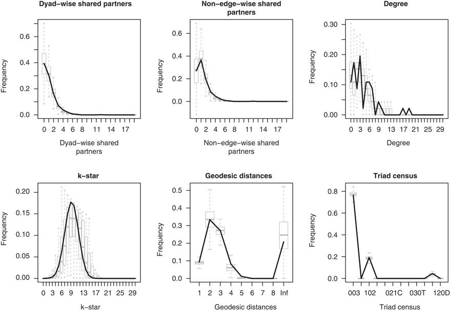
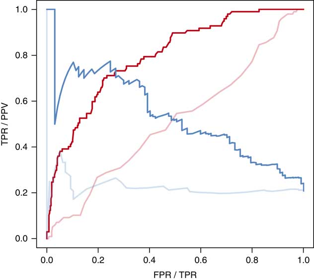
Figure 7 shows ROC curves (red curve from bottom left to top right) and PR curves (blue curve from top left to bottom right), with the light-shaded curves representing a null model for comparison. Both curves indicate a much better model fit in terms of classification performance of dyads than the null model, which means that the model has quite some explanatory value. The MCMC diagnostics (not reported here) indicate convergence, with a slight but yet unproblematic skewness for the isolates term.
Within-sample predictive fit. Receiver-operating characteristic (ROC) curves (red curve from bottom left to top right) and precision-recall (PR) curves (blue curve from top left to bottom right), with the light-shaded curves representing a null model for comparison. Note: ROC and PR are two alternative measures for model fit that indicate to which extent simulations based on the model can reproduce the location of ties in the network (Leifeld et al. Reference Leifeld, Cranmer and Desmarais2018). ROC curves trending towards the upper left corner indicate a good within-sample predictive performance of the model (=high true positive rate and low false positive rate of the simulated networks in terms of tie prediction). PR curves trending towards the upper right corner indicate a good within-sample predictive performance (=high precision and high recall of the rejection ties in the observed network). Both curves show a large difference between a null model and Model 2.
Online Appendix 2 contains additional model specifications, which rule out the possibility of multicollinearity (Model 2a), consider alternative explanations like the clustering of instruments into overarching instrument categories (Models 2b–2e), the special role of decisionmakers like governmental actors and parties and their instrument choices (Model 2f), geographical clustering of policy preferences (Model 2g), actor type homophily as a variable that may cluster actors’ preferences (Model 2h), and assess the outcomes of a different estimation technique (Model 2i). In short, none of these qualifications changes the main substantive results presented here, with the possible exception of clustering instrument preferences by overarching categories: if one assumes that every instrument is an indicator of a more general policy approach and if one controls for clustering within these approaches (regulatory, market-based and information-based, see Table 1), then in this one model specification, interconnectedness drops out of significance because the additional clustering takes away some of the residual variance that can be modelled using our main hypotheses. Conflict lines, however, still remain significant predictors of instrument preferences.
Discussion and conclusion
In order to understand how policy actors strategically position themselves in water protection given the choices of others, we studied actors’ preferences for policy instruments as an interdependent system. We modelled the social interdependencies by conceptualising policy preferences as a two-mode network of actors and their instrument preferences for pollution reduction measures. By fitting an ERGM, we studied the mechanisms behind the formation of policy preferences. Thereby the article contributes to the literatures on collective decisionmaking, policy preferences, and networks. Our first contribution is that we find evidence for network interdependencies between actors’ policy preferences through considerable clustering in the actor-instrument network. The two-mode network lens offers a particularly sound approach to the study of preference formation as it has the ability to capture the complex and interdependent system of actors and their preferences.
The network dependence at work might take the form of diffusion of preferences among actors. However, causality cannot be disentangled in a cross-sectional study (and usually not with temporal data unless they are nearly continuously observed; see Malang et al. Reference Malang, Brandenberger and Leifeld2017). Consequently, it may be plausible that factors like collaboration are not solely the cause, but also a consequence of similar preferences. Future research should adopt a fine-grained longitudinal perspective on instrument preferences in order to examine the temporal pattern of policy instrument diffusion and separate it from social selection. To achieve this goal, either advances in the temporal measurement of organisational preferences or experimental design will be necessary.
Our second contribution is that we empirically studied the relationship between individual-level and group-level foundations of preference formation. On the individual level, we considered actors’ attributes in the form of shared objectives (as in Hypothesis 1), and on the group level, we considered relational effects trough collaboration (Hypothesis 2). With regard to relational effects, we observe that interconnected actors, who collaborate with each other, tend to exhibit interdependent policy preferences (confirmation of Hypothesis 2). Pertaining to attribute-based effects, we find that instrument preferences are partly conditional on others who exhibit similar functional roles and responsibilities (partial confirmation of Hypothesis 1). This is a form of political homophily or heterophily (McPherson et al. Reference McPherson, Smith-Lovin and Cook2001). However, we do not find any evidence for political homophily in the form of shared policy objectives or agenda priorities. Homophily effects in the form of shared beliefs are well-documented (Zafonte and Sabatier Reference Zafonte and Sabatier1998; Gerber et al. Reference Gerber, Henry and Lubell2013; Calanni et al. Reference Calanni, Siddiki and Weible Cand Leach2014; Ingold and Fischer Reference Ingold and Fischer2014). The cited studies find evidence that actors who share beliefs tend to collaborate, but they do not investigate the consequences of collaboration on preference formation. Our results contribute to closing this gap by analysing both the role of underlying objectives and collaboration in preference formation. Findings indicate that actors’ objectives defined by their functional roles (as operationalised by Hypothesis 1c), and actors’ interconnectedness (as operationalised by Hypothesis 2a), play a role in shaping the collective preferences of a nascent policy domain. As alternative operationalisations of interconnectedness (Hypotheses 2b–2c) and policy objectives (Hypotheses 1a–1b) did not yield significant results, we conclude that those variables operate through specific mechanisms. With our study, we contribute to conceptual precision around these mechanisms.
Policy decisions are not merely in the hands of selected public officials or authorities, but take place in a governance structure involving different public and private actors. In such complex settings, agreement upon which instruments to select and which ones to reject represents an important precondition to successfully produce policy outputs and overcome collective action problems. Future research should investigate in a longitudinal design whether actors use their collaboration ties as a mechanism of preference coordination and compromise settlement. If this were not the case, that is, if actors formed their instrument preferences on the basis of their own fixed objectives only, producing policy outputs would be very difficult where actors with conflicting objectives participate in decisionmaking. But, our results indicate that not only functional roles, but also interconnectedness matters for the formation of policy preferences. Hence, actors can overcome their differences and successfully agree on policies when they initiate connections and exchanges during policy negotiations. In summary, where policy preferences depend both on fixed roles (as indicated by Hypothesis 1c) and collaboration (Hypothesis 2a), policymaking is both a function of who participates in policymaking and a matter of negotiation and, hence, compromise-seeking.
Finally, our results indicate that deliberation, if it matters in policy instrument preference formation, is constrained to direct collaboration between actors rather than international forums. Future research should seek to evaluate the precise relationship between coordination through policy forums and direct collaboration between actors and the consequences for preference formation.
Supplementary material
To view supplementary material for this article, please visit https://doi.org/10.1017/S0143814X18000181
Data
Replication materials are available at https://dataverse.harvard.edu/dataset.xhtml?persistentId=doi:10.7910/DVN/SX7ESZ
Acknowledgements
The authors would like to thank the Swiss National Science Foundation for their generous support (grant number CR21I1L_146336, “CrossWater – Transboundary Micropollution Regulation in Europe: The Definition of Appropriate Management Scales – An Interdisciplinary Approach”; grant number 105217_140395, “How to explain instrument selection in complex policy processes”; and grant number 149410, “Overlapping Subsystems: Identification and Integration of Fragmented Games in Swiss Water Politics”). The authors are grateful for insightful comments by Hans Bressers and the members of the Policy Analysis and Environmental Governance group at University of Berne including Laurence Brandenberger, Laura Herzog, and Lorenz Kammermann. Three anonymous reviewers provided thoughtful inputs and helped to improve our article. A previous version of this article was presented at the European Conference on Social Networks, 14–17 June 2016, Paris. The authors would like to thank conference discussants and panel members for their helpful thoughts on our article.