2.1. The LES method

In this work, the transient flow field surrounding a wind turbine is computed using LES. The governing equations are the filtered incompressible Navier–Stokes equations,

(2.1) \begin{align}&\qquad\qquad\qquad\qquad \frac {\partial \tilde {u}_i}{\partial x_i}=0, \end{align}

(2.2) \begin{align}& \frac {\partial \tilde {u}_i}{\partial t}+\tilde {u}_j\frac {\partial \tilde {u}_i}{\partial x_j}=-\frac {1}{\rho }\frac {\partial \tilde {p}}{\partial x_i}+\nu \frac {\partial ^2\tilde {u}_i}{\partial x_j\partial x_j}-\frac {\partial \tau _{ij}}{\partial x_j}+\widetilde {f_i}, \end{align}

where the subscripts $i$ and $j\,(=$ 1, 2, 3) denote the directions in the Cartesian coordinate system, $\tilde {u}_i$ represents the filtered velocity component in the $i$ th direction, $\rho$ is air density, $\tilde {p}$ stands for the filtered pressure, $\nu$ is air kinematic viscosity, $\tau _{ij}=\widetilde {u_i u_j} - \tilde {u}_i \tilde {u}_j$ is the subgrid-scale stress tensor, and $\tilde {f}_i$ is the filtered body force characterising the effects of a wind turbine on the flow.

In the present study, we employ a high-fidelity opensource pseudospectral code LESGO (Stevens, Graham & Meneveau Reference Stevens, Graham and Meneveau2014) in the present study, which has been widely used in simulations of ABL (Porté-Agel et al. Reference Porté-Agel, Meneveau and Parlange2000; Yang et al. Reference Yang, Chen, Hu and Abkar2022), wind turbine flow (Li et al. Reference Li, Zhi, Ge and Zhang2021; Narasimhan, Gayme & Meneveau Reference Narasimhan, Gayme and Meneveau2022) and wind farm flow (Calaf, Meneveau & Meyers Reference Calaf, Meneveau and Meyers2010; Liu & Stevens Reference Liu and Stevens2021). In this code, the governing equations are discretised by the pseudospectral method in the streamwise and spanwise directions, and the second-order central finite difference method is used in the vertical direction. The time advancement is conducted using a second-order accurate Adams–Bashforth scheme. The scale-dependent Lagrangian dynamic Smagorinsky model is used to calculate the subgrid-scale stress (Bou-Zeid, Meneveau & Parlange Reference Bou-Zeid, Meneveau and Parlange2005). In our previous studies (Wang et al. Reference Wang, Wang, Hu, Kong and Cheng2021), the code has been well validated by comparison with the numerical simulation results conducted by Stevens, Martinez-Tossas & Meneveau (Reference Stevens, Martinez-Tossas and Meneveau2018) and the wind tunnel measurements carried out by Chamorro & Porté-Agel (Reference Chamorro and Porté-Agel2010).

2.2. Actuator line model

The ALM is adopted to represent the effects of the wind turbine on flow (Sørensen & Shen Reference Sørensen and Shen2002). According to previous studies (Ivanell et al. Reference Ivanell, Mikkelsen, Sørensen and Henningson2008; Troldborg et al. Reference Troldborg, Sorensen and Mikkelsen2010; Sørensen Reference Sørensen2011; Martínez-Tossas et al. Reference Martínez-Tossas, Churchfield and Leonardi2014; Martínez-Tossas & Meneveau Reference Martínez-Tossas and Meneveau2019), the ALM is a suitable approach to forecasting unsteadiness and turbulent structures in the wake of wind turbines. It can accurately predict the instability of tip vortices under uniform inflows, similar to the actuator surface model (Yang et al. Reference Yang, Hong, Barone and Sotiropoulos2015), while with a significantly lower computational cost (Li et al. Reference Li, Zhang and Zhao2022c ). In the ALM, a wind turbine blade is represented by an actuator line consisting of a force distribution that extends from the hub to the tip of the blade. This continuous actuator line is divided into a finite number of blade elements or segments, with some crucial attributes associated with each element, including the airfoil type, chord length and twist angle. A look-up table for the lift and drag coefficients of the airfoil at different angles of attack should be established in advance. The local lift and drag coefficients at each blade element can be calculated depending on the local wind velocity and angle of attack. Then the local aerodynamic forces are projected into the filtered Navier–Stokes equations as body forces.

In the ALM, the lift and drag forces at each blade element are calculated as

(2.3) \begin{equation} {L}=\tfrac {1}{2}C_L\rho V_{\textit{rel}}^{2}cw, \quad {D}=\tfrac {1}{2}C_D\rho V_{\textit{rel}}^{2}cw, \end{equation}

where $L$ and $D$ are the lift and drag forces acting on each blade element, $C_L$ and $C_D$ are the lift and drag coefficients corresponding to the local angle of attack, $V_{\textit{rel}}$ is the local relative velocity between the wind and the blade, $c$ is the chord length of the airfoil and $w$ is the width of the blade element. To avoid numerical oscillations during the computation, the body force needs to be smoothly projected into the surrounding fluid cells by means of a three-dimensional Gaussian function (Troldborg et al. Reference Troldborg, Sorensen and Mikkelsen2010) ,

(2.4) \begin{equation} f=\frac {{F}}{\pi ^{{3}/{2}} \varepsilon ^3}\exp \left [ -\left ( \frac {d}{\varepsilon } \right )^2 \right ], \end{equation}

where $f$ is the smoothed body force, $F$ is the body force of each element, $\varepsilon$ is the projection radius of the Gaussian function and $d$ is the distance from the centre of a blade element to a point in the flow.

To clarify the uncertainties that affect the characteristics of the wake, we consider the impact of a nacelle in our simulations, as it may significantly alter the wake (Abraham, Dasari & Hong Reference Abraham, Dasari and Hong2019). In the present study, the nacelle is modelled similarly to the actuator disk model, with the body forces derived from the nacelle model incorporated into the momentum equation. The body force $f_{nac}$ is

(2.5) \begin{equation} f_{nac}=\tfrac {1}{2}\rho U_{nac}^{2}C_{D,nac}A_{nac}, \end{equation}

where $U_{nac}$ represents the axial velocity in front of the nacelle, $C_{D,nac}$ is the drag coefficient of the cylinder and $A_{nac}$ refers to the projected area of the nacelle in its rotational plane. For further information on the current implementation of the nacelle model, one can refer to the study by Stevens et al. (Reference Stevens, Martinez-Tossas and Meneveau2018).

Although wind turbine towers can affect the asymmetry of the wake, particularly in the bottom of the near wake (Santoni et al. Reference Santoni, Carrasquillo, Arenas-Navarro and Leonardi2017; Abraham et al. Reference Abraham, Dasari and Hong2019), their influence is relatively weak in the far-wake region compared with the unstable hub vortices generated by the nacelle. Schümann et al. (Reference Schümann, Pierella and Sætran2013) found that when turbines operate within the wakes of upstream turbines, the tower vortices become negligible in the far wake and are considerably weakened in the near wake. Furthermore, due to the relatively small size of a tower compared with that of a turbine rotor, a higher grid resolution is needed to resolve the flow close to the tower, which is computationally much more prohibitive. Considering that the main objective of this study is to quantitatively assess the impact of TSR on wake meandering, as well as our limited computational resources, the presence of a tower is not considered in the present numerical simulations.

2.3. Concurrent precursor method

The concurrent precursor method of Stevens et al. (Reference Stevens, Graham and Meneveau2014) is adopted to generate the inflow under the ABL condition. Two simulations are conducted concurrently. The first simulates a flow without a wind turbine using a periodic condition and imposing a pressure gradient in the streamwise direction, and it is termed the precursor domain. The second one conducts a simulation with a wind turbine, and is referred to the main domain. The sizes of the two domains are exactly the same. The flow field at the end of the precursor domain (the fringe region) is transferred to the main domain as an inflow in the absence of turbine wake. Additionally, placing the fringe region at the end of the domain aims to preclude unnecessary oscillations and ensure a smooth transfer. It is also noted that the grid spacing and time step for both domains are the same, allowing the direct transfer of the flow field without the need for interpolation.

In the concurrent precursor method, the velocity in the fringe region of the main domain is determined as

(2.6) \begin{equation} {\mathbf{u}(x,y,z,t) = {w}(x)\cdot \mathbf{u}_{{pre}}(x,y,z,t) + (1-{w}(x))\cdot \mathbf{u}_{\textit{LES}}(x,y,z,t)}, \end{equation}

in which, $\mathbf{u}_{{pre}}$ is the velocity field of the precursor domain, $\mathbf{u}_{\textit{LES}}$ is the velocity field of the main domain before transfer, $w(x)$ is a weighting function defined as

(2.7) \begin{equation} w(x) = \begin{cases} \dfrac {1}{2} \left [ 1 - \cos \left ( \pi \dfrac {x - L_s}{L_{pl} - L_s} \right ) \right ], & \text{if } x \gt L_s \text{ and } x \lt L_{pl}, \\ 1, & \text{if } x \gt L_{pl} \text{ and } x \lt L_x, \end{cases} \end{equation}

where $L_s=7L_x/8$ , $L_{pl}=L_x-1/4L_f$ , $L_f=L_x/8$ and $L_x$ is the streamwise length of the domain.

2.4. Simulation set-up

In this study, the simulation is carried out within a rectangular domain, as shown in figure 1. The size of the computational domain is $L_x\times L_y\times L_z=25D\times 5D\times 5D$ , where $L_x, L_y$ and $L_z$ are the lengths of the computational domain in the streamwise $(x)$ , spanwise $(y)$ and vertical $(z)$ directions, respectively. A three-blade horizontal-axis wind turbine is used, i.e. the standard NREL 5 MW wind turbine, with a rotor diameter of 126 m and a rated wind speed of 11.4 m s⁻¹. In the present study, the nacelle is modelled as a drag-only actuator disk (Wu & Porté-Agel Reference Wu and Porté-Agel2011; Aitken et al. Reference Aitken, Čosić, Mirocha and Lundquist2014; Stevens et al. Reference Stevens, Martinez-Tossas and Meneveau2018). Two nacelle models of different sizes are analysed: one with a diameter of 2.5 m ( $\sim 0.02D$ ) and the other with a diameter of 25 m ( $\sim 0.2D$ ). The length of the nacelle is 1 m. The wind turbine is located in the centre of the $x{-}y$ plane with $4D$ downstream of the inlet in the $x$ direction.

Figure 1.

Schematic diagram of the simulation domain.

In this study, two distinct inflow conditions are invoked: a uniform inflow and an ABL inflow. Under the uniform inflow, the lateral boundaries of the simulation domain are subject to a stress-free condition. In the streamwise direction, the flow is driven by a pressure gradient and a periodic condition is applied to the inlet and outlet boundaries. A uniform inflow of $U_{\infty }= 11.4$ m s⁻¹ in accordance with the design-rated wind speed is introduced at the inlet. The wind turbine is placed at $z=2.5D$ from the bottom of the domain, i.e. the middle of the domain height. The flow in the fringe region, i.e. the last $4D$ in the streamwise direction, is enforced to the uniform inflow. Under the ABL inflow, the periodic boundary condition is adopted in the streamwise and spanwise directions combined with the concurrent precursor method, while the upper boundary in the vertical direction is assigned a stress-free condition, and the lower boundary is equipped with an equilibrium wall model (Porté-Agel et al. Reference Porté-Agel, Meneveau and Parlange2000; Bou-Zeid et al. Reference Bou-Zeid, Meneveau and Parlange2005). In addition, the friction velocity is 0.4 m s⁻¹, and the boundary layer thickness $\delta$ = 1000m, which serves as the reference velocity and the length scales, respectively. The simulation covers a domain with the wind turbine positioned at $z=90$ m from the bottom surface. The mean flow velocity at the turbine centre is approximately 11.4 m s⁻¹. The inflow characteristics of the precursor simulation is not given a priori but obtained from the simulation results a posterior under the ABL condition. In the precursor simulation, a pressure gradient was applied in the main flow direction to generate a fully developed ABL. At this stage, periodic boundary conditions were applied in both the $x$ and $y$ directions. The total kinetic energy in the flow was monitored to ensure that the turbulent boundary layer achieved a fully developed state before the collection of the flow data. The magnitude of the mean pressure gradient is determined by the friction velocity, as it is balanced by the wall friction.

A uniform Cartesian grid is employed with a resolution of 5 m $\times$ 5 m $\times$ 5 m, and the total number of grids in the simulation domain is $N_x\times N_y\times N_z=630\times 126\times 126$ . In order to maintain a smooth application of the body force, the time step $\Delta t$ is kept a constant 0.025 s in the simulation. This ensures that the movement of the blade tip does not cross over one grid cell during each time step. The turbine blade is discretized into 60 elements, meeting the minimum requirement of 40 actuator elements per blade of the ALM method (Martínez-Tossas et al. Reference Martínez-Tossas, Churchfield and Leonardi2014). To avoid numerical oscillations throughout the computation, $\varepsilon$ is set to 12.5, which is more than twice the grid size, in accordance with Troldborg, Sorensen & Mikkelsen (Reference Troldborg, Sorensen and Mikkelsen2007).

The TSRs investigated in the present study range from 5 to 8, with TSR = 7 being the optimal TSR with the highest efficiency of wind energy harvesting. In the uniform inflow cases, we sampled the flow field once it was fully developed and became statistically stationary after the initial transient with an interval of 0.25 s, which leads to a sampling frequency of 4 Hz for the subsequent statistical analysis. More specifically, the data used in the present study were sampled in a total of $\Delta T=1500$ s and $N=6000$ instantaneous snapshots. In the ABL inflow cases, the flow was fully developed and reached a statistically stationary state at $t=45\,000$ s after the initial transient. Consequently, it was sampled with an interval of 0.25 s and a sampling frequency of 4 Hz for subsequent statistical analysis. Specifically, the data utilised in this study were sampled from $t=4\,45\,500$ s to 4 48 000 s ( $\Delta T=2500$ s), resulting in a total of 10 000 instantaneous snapshots.

Figure 2(a) shows the mean streamwise velocity profile at the inlet of the main domain under the ABL condition. It can be seen that the mean velocity distribution in the logarithmic layer ( $z\lt 0.2\delta$ ) is well fitted by the logarithmic law. Figure 2(b) displays the profile of the turbulence intensity $TI$ at the inlet, which is defined as

(2.8) \begin{equation} TI = \frac { \sqrt { \overline {u^{\prime 2}} + \overline {v^{\prime 2}} + \overline {w^{\prime 2}} } }{ \overline {U}}, \end{equation}

where $\overline {u^{\prime 2}}$ , $\overline {v^{\prime 2}}$ , $\overline {w^{\prime 2}}$ are the intensities of the velocity fluctuations in the $x$ , $y$ and $z$ directions, respectively, $\overline {U}$ is the mean velocity of the inflow. It can be seen that the turbulent intensity of the inflow at the hub height is approximately 12 %.

Figure 2.

Profiles of the mean streamwise velocity and turbulence intensity under the ABL inflow.

Figure 3.

Two-point correlation coefficients (a) and the integral scales (b) of the streamwise velocity fluctuation at different heights in the precursor domain.

To further inspect the turbulence characteristics in the freestream, we compute the two-point correlation coefficient and the integral scale of the flow in the precursor domain, as depicted in figure 3. The two-point correlation coefficient of the streamwise flow velocity fluctuation is defined by

(2.9) \begin{equation} R_{u^\prime u^\prime }(\Delta x) = \frac {\overline { u^\prime (x,y,z) \, u^\prime (x+\Delta x,y,z) }}{\sigma _{u^\prime (x,y,z)} \, \sigma _{u^\prime (x+\Delta x,y,z)}}, \end{equation}

where $u^\prime$ is the streamwise velocity fluctuation, the overline denotes ensemble average, $\sigma _{u^\prime }$ is the standard deviation of the streamwise velocity fluctuation. Figure 3(a) shows the two-point correlation coefficient of the streamwise flow velocity fluctuation along the streamwise direction at different heights ( $z$ = 15 m to 280 m). Then, the streamwise integral scale can be obtained by (Pope Reference Pope2000)

(2.10) \begin{equation} L_u = \int _{0}^{\infty } R_{u^\prime u^\prime }(\Delta x) \, \mathrm{d}\Delta x. \end{equation}

Figure 3(b) displays the streamwise integral scales at different heights, which is approximately 0.03 $\delta$ at the hub height.

3.1. Basic characteristics

To analyse the basic characteristics of wake meandering, the mean velocity deficit, instantaneous velocity deficit and vorticity distribution of the wake under the uniform inflow in the $x$ - $y$ plane at the hub height are presented in figure 4, in which the optimal TSR = 7 is chosen as a representative case. In figure 4(a), the time-averaged field of the streamwise velocity deficit, i.e. $\overline {\Delta {u}}=U_{\infty }-\overline {\tilde {u}}$ , is shown. It can be seen that the mean velocity deficit distribution of the wake is straight and nearly symmetrical along the streamwise central line. There is a noticeable velocity deficit in the area of $0\lt x\lt 9D$ , and the wake slowly recovers at $x\gt 9D$ , where the wake expands and the velocity deficit gradually diminishes. Figure 4(b) portrays the instantaneous streamwise velocity deficit distribution $\Delta u=U_{\infty }-{\tilde {u}}$ in the wind turbine wake at $t=1500$ s. The red dash–dotted line represents the geometric centre of the wind turbine wake, which is extracted using the Gaussian fitting method (Li et al. Reference Li, Zhang and Zhao2022b ),

(3.1) \begin{equation} \Delta u(x,y)=\Delta u_c\left ( x \right ) \exp \!\:\left [ -\frac {\left ( y-y_c\left ( x \right ) \right ) ^2}{2\sigma ^2\left ( x \right )} \right ], \end{equation}

where $\Delta u_c$ is the peak of the velocity deficit after the Gaussian fitting, $\sigma (x)$ is the standard deviation of the Gaussian distribution fitted with the velocity profile and $y_c(x)$ is the geometric centre of the wake, defined as the spanwise position corresponding to $\Delta u_c(x)$ . It can be seen that the instantaneous turbine wake is very similar to that of the mean velocity deficit distribution within the near wake region of around $0\lt x\lt 6D$ , i.e. the wake is straight and no meandering motion can be observed. In the downstream of $6D\lt x\lt 9D$ , the wake starts meandering gradually and demonstrates slight meandering amplitudes. When the wake propagates to the far wake region of $x\gt 9D$ , substantial lateral motions of the wake become prominent, signifying a distinct meandering motion in the wind turbine wake. Figure 4(c) depicts the vorticity distribution of the wind turbine wake identified using the $Q$ criterion (Hunt, Wray & Moin Reference Hunt, Wray and Moin1988), in which $Q$ is the second invariant of the flow velocity gradient tensor. There are obvious tip and root vortices that can be observed in the near-wake region of $x\lt 9D$ . These tip and root vortices almost have no meandering motions within the near-wake region. At $x\gt 9D$ , the vortices become unstable and their fluctuation amplitudes increase as they go downstream. Eventually, the vortices merge and disintegrate.

Figure 4.

Contours of (a) mean velocity deficit $\overline {\Delta u}$ , (b) instantaneous velocity deficit $\Delta u$ at $t=1500 {\rm s}$ and (c) the second invariant of velocity gradient tensor $Q$ in the $x{-}y$ plane across the turbine hub at TSR = 7.

To examine the evolution and meandering amplitudes of the turbine wake quantitatively, several probing points are placed in the flow field. They are at six locations of $x/D=0,3,6,9,12$ and 15 along the wake centreline behind the turbine rotor in the downstream, and six locations at the tip and half of the blade of $y/D=0.25$ and 0.5 in the spanwise and $x/D=0,12$ and 15 in the streamwise, as shown by the symbols in figure 4(b). Statistical analysis of the spanwise velocity fluctuation at these points is conducted, and their power spectral density functions $\psi _{v'}$ are presented in figure 5 and figure 6.

Figure 5.

Power spectral densities of spanwise velocity fluctuation $\psi _{v^\prime }$ at different streamwise locations of the wake centreline with TSR = 7.

In figure 5, the power spectral densities of the spanwise velocity fluctuations $\psi _{v'}$ at the points of $y/D=0$ along the wake centreline are presented. It can be seen that there is a pronounced peak in the low-frequency range for all sampling points except $x/D$ = 0. Specifically, the peak in $\psi _{{v'}}$ has a frequency of $f_k=0.0156$ Hz ( $St=0.17$ ) corresponding to the characteristic frequency of the wake meandering. The peak power spectral density and broadband spectral energy continuously grow with increasing downstream length $x$ and gradually saturate at approximately $x/D\gt 9$ , indicating that both the low-frequency wake meandering and broadband turbulence have been fully developed.

Figure 6.

Power spectral densities of spanwise velocity fluctuation $\psi _{v^\prime }$ at different spanwise locations with TSR = 7: (a) $x/D$ = 0; (b) $x/D$ = 12; (c) $x/D$ = 15.

On the other hand, two distinct peaks are observed at a higher frequency of $f_n=0.21$ Hz ( $St=2.32$ ) at $x/D=0$ , which is the same as the rotation frequency of the rotor, as well as its second harmonic, accompanied by a higher energy band between $f_n$ and $2f_n$ . As displayed in figure 6(a), the amplitudes of the two higher frequency peaks grow from $y/D=0$ to $y/D=0.5$ . This corresponds to the tip vortices so that the peak amplitude is greater when the sample point is closer to the blade tip. In the downstream of $x/D=12$ and $x/D=15$ , the peaks of the power spectral density functions $\psi _{v^\prime }$ at $y/D=0$ , $y/D=0.25$ and $y/D=0.5$ are well collapsed to the characteristic frequency $f_k=0.0156$ Hz ( $St=0.17$ ) of wake meandering, as shown in figures 6(b) and 6(c). Nevertheless, at $x/D=15$ , the spectral energy in the high-frequency bands of $\psi _{v^\prime }$ is significantly higher than that at $x/D=12$ , suggesting that the broadband turbulence is still developing and the turbulence kinetic energy is transferred from the low-frequency large-scale structures to the high-frequency small-scale structures through the energy cascade process. Indeed, it is evident that the spectrum at $x/D=15$ exhibits an inertial range that more closely adheres to the $-5/3$ power law compared with that at $x/D=12$ .

3.2. Effects of TSR

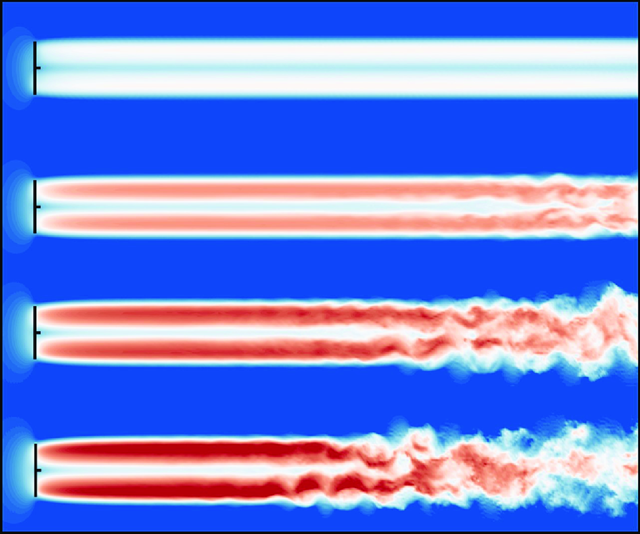
Figures 7(a), 7(c), 7(e) and 7(g) show the instantaneous distributions of the wake velocity deficit of wind turbines with TSR = 5, 6, 7 and 8 under the uniform inflow. It indicates that significant wind turbine wake meandering occurs in all cases except TSR = 5, which may be attributed to the limitation of the domain size. The effect of simulation domain size at TSR = 5 is dissected in Appendix A. The wake meandering is more intense and starts earlier as the TSR increases, as depicted by the arrows in figure 7, which agrees with previous observations (Troldborg et al. Reference Troldborg, Sorensen and Mikkelsen2010; Felli et al. Reference Felli, Camussi and Felice2011; Sherry et al. Reference Sherry, Nemes, Lo Jacono, Blackburn and Sheridan2013; Kleusberg et al. Reference Kleusberg, Schlatter and Henningson2020) in the instability and breakdown of tip vortices, while here we demonstrate that a higher TSR also triggers an earlier onset of wake meandering. Figures 7(b), 7(d), 7(f) and 7(h) display the vorticity distributions of the wind turbine wake with TSR = 5, 6, 7 and 8 at the same time. When TSR = 5, the wake structure consists mostly of dominant blade tip vortices and less intense root vortices. These vortices are relatively stable and do not exhibit significant mixing or interaction until a distance of $x/D$ = 15. As shown in figures 7(d), 7(f) and 7(h), the wake structure becomes more unstable as TSR grows. At TSR = 6, 7 and 8, the tip vortices and root vortices can be mixed in the distant wake region, which occurs earlier with increasing TSR.

Figure 7.

Instantaneous velocity deficit fields in the $x{-}y$ plane across the turbine hub with different TSRs at $t=2000$ s and the corresponding vorticity distributions: (a,b) TSR = 5; (c,d) TSR = 6; (e,f) TSR = 7; (g,h) TSR = 8.

Figure 8.

Instantaneous wake vortex identified by the $Q$ -criterion: (a) TSR = 5; (b) TSR = 6; (c) TSR = 7; (d) TSR = 8. The colour represents the flow velocity magnitude.

Figure 9.

Streamwise evolution of one-point statistics of the streamwise velocity fluctuation $u^\prime$ and the spanwise velocity fluctuation $v^\prime$ in the centreline of the wake. (a) The variance $V({{u}^\prime })$ , (b) the skewness $S({{u}^\prime })$ , (c) the kurtosis $K({{u}^\prime })$ , (d) the variance $V({{v}^\prime })$ , (e) the skewness $S({{v}^\prime })$ and (f) the kurtosis $K({{v}^\prime })$ .

Figure 10.

Power spectral densities of the spanwise velocity fluctuation $\psi _{v^\prime }$ at different locations along the wake centreline with TSR = 5, 6, 7 and 8, respectively: (a) TSR = 5; (b) TSR = 6; (c) TSR = 7; (d) TSR = 8.

To further understand the impact of TSR on the three-dimensional features of the turbine wake, we also leverage the $Q$ -criterion to identify the wake vortex, as depicted in figure 8. It is seen that the near-wake vortex predominantly comprises tip and root vortices. When TSR = 5, the wake structure remains fairly stable. As the TSR grows, the vortices approach one another and interact at varying downstream distances, ultimately leading to the breakdown of vortices and oscillations in the wake. Specifically, at TSR = 7 and 8, the vortex structure in the wake exhibits strong volatility and instability, accompanied by significant large-scale intermittency characteristics. The wake-meandering phenomenon intensifies, with its onset increasingly nearing the turbine rotor, accompanied by a substantial increase in amplitude. These results correspond to the wind turbine wake characteristics illustrated in figure 7, collectively suggesting that TSR is a pivotal parameter that influences the wake mending phenomenon. Moreover, the findings demonstrate that vortex shedding and wake vortex instability are the primary mechanisms responsible for wake meandering under the uniform inflow.

Figure 9 shows the streamwise variation of the time-averaged one-point statistics of the streamwise velocity fluctuation $u^\prime$ and the spanwise velocity fluctuation $v^\prime$ along the wake centreline at different TSRs, namely the variance $V({u^\prime })$ and $V({v^\prime })$ , the skewness $S({u^\prime })$ and $S({v^\prime })$ and the kurtosis $K({u^\prime })$ and $K({v^\prime })$ . Figures 9(a) and 9(d) illustrate the streamwise evolution of $V({u^\prime })$ and $V({v^\prime })$ . When TSR = 5, the value of $V({u^\prime })$ becomes very close to zero throughout the wake and $V({v^\prime })$ has the same pattern. This indicates that the flow velocity fluctuations in the wake are very small, and the wake meandering is not obvious. However, we can speculate on instability and wake meandering in the far wake region, as demonstrated in Appendix A. When TSR = 6, $V({u^\prime })$ and $V({v^\prime })$ start to gradually rise at nearly $x/D = 15$ . When TSR = 7 and 8, the increase in $V({u^\prime })$ starts around $x/D = 9$ , and $V({v^\prime })$ starts to increase around $x/D = 9$ and $x/D = 6$ , respectively. Furthermore, a distinct peak can be observed in both $V({u^\prime })$ and $V({v^\prime })$ for the case of TSR = 8. After the peak, the variances gradually decrease and become stable downstream, indicating the full development of the wake. The peak locations of $V({u^\prime })$ and $V({v^\prime })$ move towards the wind turbine as the TSR grows, demonstrating that the wake recovers more and more quickly. It should be noted that when TSR = 5 and 6, the wake development is significantly slow and does not reach a fully developed state due to the limited size of the simulation domain. Figures 9(b) and 9(e) show the variations in skewness $S({u^\prime })$ and $S({v^\prime })$ along the wake centreline. It can be seen that they are almost zero for all TSRs, which indicates that the wakes are symmetric. Figures 9(c) and 9(f) present the streamwise variations of kurtosis $K({u^\prime })$ and $K({v^\prime })$ along the centreline of the wake. The values of $K({u^\prime })$ and $K({v^\prime })$ are approximately 3 throughout the wake for all TSRs, suggesting that the distributions of $u^\prime$ and $v^\prime$ are close to a Gaussian distribution. The above results indicate that TSR substantially influences the evolution and growth rate of the wake meandering. However, it has little effect on the Gaussian nature of the wake.

The evolutions of the power spectral density of spanwise velocity fluctuation $\psi _{v^\prime }$ at different TSRs along the wake centreline are shown in figure 10. When TSR = 5, as shown in figure 10(a), there are three distinct peaks in the high-frequency range of $\psi _{v^\prime }$ . These peaks correspond to the rotor rotation frequency $f_n$ = 0.15 Hz ( $St=1.66$ ) and its double and triple harmonics. It aligns with the earlier observation that there is no significant occurrence of a large-scale oscillation in the wake at this TSR up to $x/D=17$ . Instead, the flow is mainly shaped by the vortices shed at the tips and roots of the turbine blades. For the other TSRs, the low-frequency peak associated with the large-scale wake meandering can be detected in $\psi _{v^\prime }$ . Without a nacelle, the frequency of this peak remains unchanged regardless of TSR, measuring 0.0156 Hz with a corresponding Strouhal number $St$ = 0.17, close to the simulation results of Foti et al. (Reference Foti, Yang, Guala and Sotiropoulos2016) with $St=0.15$ , and not very far from many measurement results, e.g. $St=0.1-0.3$ in (Medici & Alfredsson Reference Medici and Alfredsson2006), $St=0.23$ in Okulov et al. (Reference Okulov, Naumov, Mikkelsen, Kabardin and Sorensen2014) and $St=0.2-0.3$ in Biswas & Buxton (Reference Biswas and Buxton2024). It is seen that with increasing TSR, the appearance of a low-frequency peak is promoted, which is consistent with the findings in figures 7 and 9. In addition, a recent study of De Cillis et al. (Reference De Cillis, Cherubini, Semeraro, Leonardi and De Palma2022b ) analysed the wind turbine wake by SP-DMD and identified the most dynamically correlated coherent structures in the wake. It is found that the maximum amplitude DMD modes mainly composed of tip vortices, which frequency is three times that of wind turbine rotation frequency similar to the present finding with a different method. Other selected modes exhibit low frequencies of large-scale flow structures, aligning with wake meandering. These findings are highly relevant to the present results, especially the characteristics of tip and root vortices.

3.3. Effects of the ABL inflow

Figures 11(a), 11(c), 11(e) and 11(g) illustrate the instantaneous wake velocity deficits in the $x{-}y$ plane at the hub height of the wind turbine with TSR = 5, 6, 7 and 8 under the ABL inflow, respectively. It reveals that under the ABL inflow, the wind turbine wake exhibits a much earlier meandering and a notable increase in the amplitude of wake oscillations compared with the uniform inflow cases. Additionally, as the wake advances towards the far wake region, a reduction in velocity deficit can be observed, indicating a gradual recovery of the wake. In particular, an increase in TSR correlates with an increased recovery of wake velocity. The vorticity fields in the $x{-}y$ plane at the hub height of the wind turbine with various TSRs are presented in figures 11(b), 11(d), 11(f) and 11(h). It can be seen that the vortical structures in the wake are much more complex under the ABL inflow than under the uniform inflow. At TSR = 5, due to the low rotational speed of the wind turbine, the shear effect on the flow is relatively weak, as are the tip and root vortices, leading to the wake structure being predominantly dominated by the freestream turbulence. As the TSR increases, the tip and root vortices are increasingly stronger, which gradually mix in the wake and interact with the vortical structures of the ambient turbulence.

Figure 11.

Instantaneous velocity deficit fields in the $x{-}y$ plane across the turbine hub at different TSRs under the ABL inflow and the corresponding vorticity distributions: (a,b) TSR = 5; (c,d) TSR = 6; (e,f) TSR = 7; (g,h) TSR = 8.

Figure 12.

Streamwise evolution of one-point statistics of the streamwise velocity fluctuation $u^\prime$ and the spanwise velocity fluctuation $v^\prime$ in the centreline of the wake under the ABL inflow: (a) the variance $V({{u}^\prime })$ ; (b) the skewness $S({{u}^\prime })$ ; (c) the kurtosis $K({{u}^\prime })$ ; (d) the variance $V({{v}^\prime })$ ; (e) the skewness $S({{v}^\prime })$ ; (f) the kurtosis $K({{v}^\prime })$ .

Figure 12(a) and 12(d) show the streamwise evolution of the variances $V({{u}^\prime })$ and $V({{v}^\prime })$ at various TSRs, respectively. It is seen that, as the TSR increases, the value of $V({{u}^\prime })$ gradually increases, which can be attributed to the increasing interaction between the tip/root vortices and the freestream turbulence with increasing rotation speed of the wind turbine. This interaction intensifies the velocity fluctuations within the wake. Furthermore, at $x \approx 3D$ , there is an abrupt increase in the variances, suggesting the onset of a meandering under the ABL inflow. The magnitude of $V({{v}^\prime })$ is observed to be less than that of $V({{u}^\prime })$ . Figures 12(b) and 12(e) display the streamwise evolution of the skewness $S({{u}^\prime })$ and $S({{v}^\prime })$ along the wake centreline. It can be observed that, at all TSRs, the skewness essentially fluctuates around zero. Figures 12(c) and 12(f) present the evolution of the kurtosis $K({{u}^\prime })$ and $K({{v}^\prime })$ along the wake centreline. It is seen that at all TSRs, the kurtosis fluctuates around 3. Therefore, from the results of skewness and kurtosis, one can find that the wake velocities under the ABL inflow also follow the Gaussian distribution approximately.

Figure 13.

Power spectral densities of the spanwise velocity fluctuation $\psi _{v^\prime }$ and the corresponding premultiplied spectra at different locations along the centreline of turbine wake at TSR = 5, 6, 7 and 8 under the ABL inflow, respectively: (a,e) TSR = 5; (b,f) TSR = 6; (c,g) TSR = 7; (d,h) TSR = 8. The line colours are the same as those in figure 10.

To further clarify the characteristics of the wake meandering under the ABL inflow, we perform spectral analysis of the spanwise velocity fluctuations at various streamwise locations of the wake centreline. The results are depicted in figure 13. Spectral analysis reveals that the turbulent kinetic energy within the wake structure is predominantly concentrated in the low-frequency range. The spectra $\psi _{v^\prime }$ follow the $-5/3$ law at all TSRs, indicating that the turbine wake under the ABL inflow exhibits features of fully developed turbulence. To extract the dominant frequency of the wake more clearly, premultiplied spectra are further shown in figure 13(e–h). The results indicate that the premultiplied spectra display a consistent peak with a frequency of 0.0029 Hz ( $St=0.03$ ) and independent of TSR. The observation aligns with the results obtained under the uniform inflow, although with a much-reduced value of the characteristic frequency. This may be attributed to the fact that the energetic eddies in the turbulent inflow are of low frequency, which interact with the tip/root vortices in the wake, thereby influencing and leading to a decrease in the peak frequency associated with the wake meandering. Actually, we also analysed the spectra of inflow velocity and found that the peak frequency is 0.0058 Hz ( $St=0.06$ ) which is twice that in the wake. Furthermore, we find that the effects of the precursor domain size on the dominant frequency of the wake meandering can be neglected, as detailed in Appendix B.

3.4. The TSR dependence of wake meandering frequency

As we have mentioned before, there exists a controversy over the TSR effect on the characteristic frequency of wake meandering. Medici & Alfredsson (Reference Medici and Alfredsson2006, Reference Medici and Alfredsson2008) and Biswas & Buxton (Reference Biswas and Buxton2024) found a decreasing trend of $St$ with TSR, while Okulov et al. (Reference Okulov, Naumov, Mikkelsen, Kabardin and Sorensen2014) observed a constant $St$ . Biswas & Buxton (Reference Biswas and Buxton2024) suspected that the result of Okulov et al. (Reference Okulov, Naumov, Mikkelsen, Kabardin and Sorensen2014) may be affected by the long-arm-like nacelle. The present simulation results for the wind turbine without a nacelle support the finding of Okulov et al. (Reference Okulov, Naumov, Mikkelsen, Kabardin and Sorensen2014), i.e. the $St$ of wake meandering is independent of TSR. Furthermore, we also conduct simulations of wind turbines with a nacelle of different sizes, and the results are shown in the figure 14. Figure 14(a) illustrates the variation of $St$ of wake meandering with TSR under the uniform inflow for three cases: no nacelle; a small nacelle (diameter $\sim 0.02D$ ); a large nacelle (diameter $\sim 0.2D$ ). The characteristic frequency and $St$ of $\psi _{v^\prime }$ are independent with TSR in the cases of no nacelle and a small nacelle, while exhibiting an increasing trend first and then a decreasing trend with TSR in the case of a large nacelle. Figure 14(b) depicts the variation of $St$ of the wake meandering with TSR under the ABL inflow for two scenarios: one without a nacelle and the other with a large nacelle (diameter $\sim 0.2D$ ). The trend of variation of $St$ with TSR is consistent with the results under the uniform inflow condition. That is, without a nacelle, $St$ remains constant, and in the presence of a large nacelle, $St$ increases first and then decreases with TSR. It is also seen that the $St$ of the wake is much smaller under the ABL inflow than under the uniform inflow, which is 0.03 without a nacelle. We found that the $St$ corresponding to the peak frequency of the inflow turbulence is 0.06, which is approximately twice that of the wake. Therefore, the low-frequency wake under the ABL condition is probably caused by the large-scale inflow turbulence, suggesting that the atmospheric turbulent structures in the inflow overwhelm the tip/root vortex as the dominant mechanism of wake meandering under the ABL condition. In conclusion, the TSR dependence of $St$ can be affected by the presence of a large nacelle. Moreover, although the flow structures and the characteristic frequency of the wake are quite different under the two inflow conditions, the general trend of $St$ with TSR remains consistent regardless of whether a nacelle is included or not.

Figure 14.

Variations of the Strouhal number of wake meandering against TSR for the cases with and without a nacelle: (a) The uniform inflow; (b) the ABL inflow.

4.1. Proper orthogonal decomposition analysis

The spatial distributions and temporal evolution characteristics of the energy-containing modes in a turbine wake can be effectively investigated using the proper orthogonal decomposition (POD) method. The POD technique, initially suggested by Lumley (Reference Lumley1967) for the detection of energetic structures in flow fields, is an effective method to reduce the dimensionality of the problem. This is achieved by separating the spatial and temporal characteristics of the flow field, requiring only minimal computational resources. Applying the usual POD approach directly to our LES, which consists of $10 \times 10^6$ grid nodes, would be excessively expensive. To tackle this challenge, we employ the snapshot POD method pioneered by Sirovich (Reference Sirovich1987), which involves performing a singular value decomposition on the flow field via a sequence of snapshots. This variant of the POD technique has gained significant popularity over the past several decades and has become a common choice for analysing flows in various applications (Rowley & Dawson Reference Rowley and Dawson2017; Taira et al. Reference Taira, Brunton, Dawson, Rowley, Colonius, McKeon, Schmidt, Gordeyev, Theofilis and Ukeiley2017).

In the snapshot POD method, the time series of the velocity deficit fluctuation is decomposed into a linear combination of discrete spatial modes and time coefficients, as

(4.1) \begin{equation} \Delta {{u}}^\prime \left ( x,y,z,t \right )=\sum _{i=1}^n a_i\left ( t \right ){\phi _i\left ( x,y,z \right )}, \end{equation}

where $\Delta {{u}}^\prime$ is the fluctuation of $\Delta {u}$ ( $\Delta {{u}}^\prime =\Delta {u}-\overline {\Delta {u}}$ ); $\phi _i$ represents the $i$ th POD mode, where $i=1, 2, 3,\ldots ,n$ is the mode number; $a_i(t)$ is the time coefficient corresponding to each mode, reflecting the temporal evolution characteristics of the spatial mode. Here $a_i(t)$ can be determined using the following projection method, as

(4.2) \begin{equation} a_i(t)=\langle {\Delta u'}\left (x, y , z, t\right ), \phi _i\rangle . \end{equation}

Here the bracket $\langle \cdot \rangle$ is the inner product. The ordering of $\phi _i$ is dictated by their corresponding eigenvalues $\lambda _i$ , where the magnitude of these eigenvalues signifies the corresponding energy contribution of the $i$ th mode.

4.1.1. The uniform inflow cases

To more intuitively illustrate the relative significance and cumulative impacts of various modes on the total energy of the wake, we normalised the energy of the first 20 POD modes at various TSRs, as shown in figure 15. The left-hand axis presents the energy contributions, defined as the ratio of $\lambda _i/\sum {_{i=1}^{N}}\lambda _i$ , while the right-hand axis illustrates the cumulative energy contributions, as the ratio of $\sum {_{i}}\lambda _i/\sum {_{i=1}^{N}}\lambda _i$ . Among all TSRs, the lower-order modes (with $i\leqslant 6$ ) display a clear step-like distribution, which is a typical characteristic of quasiperiodic signals. It is also worth noting that among the POD modes, the energy contribution of the first two modes, $\lambda _1$ and $\lambda _2$ , is almost equal and significantly higher than the other modes. Therefore, we identify these two modes as the dominant modes in the subsequent analysis.

Figure 15.

Energy contributions and cumulative energy ratios corresponding to the first 20 POD modes at different TSRs under the uniform inflow: (a) TSR = 5; (b) TSR = 6; (c) TSR = 7; (d) TSR = 8.

Figure 16.

Vorticity distributions of the first two POD modes (a,c,e,g) $\phi _1$ and (b,d,f,h) $\phi _2$ at different TSRs under the uniform inflow: (a,b) TSR = 5; (c,d) TSR = 6; (e,f) TSR = 7; (g,h) TSR = 8.

Figure 16 illustrates the spatial vorticity distributions of the first and second POD modes at various TSRs in the $x{-}y$ plane at the hub height. It is evident that the first two modes exhibit a high degree of similarity. The similarity arises from the fact that a single POD mode is insufficient to capture a particular flow structure. However, by slightly shifting a POD mode along the flow direction while maintaining the same spatial distribution, it is generally possible to characterise a specific flow structure. When TSR = 5, the primary POD modes are observed to consist of stable tip and root vortices, which closely resemble the original flow field. Nevertheless, the structures of the dominant POD modes exhibit distinct spatial properties for TSR = 6, 7 and 8. As the downstream distance increases, the two groups of root and tip-vortex structures gradually become unstable and finally mix in the far wake region. Furthermore, there is noticeable dissipation in the cases of TSR = 7 and 8. A similar phenomenon was also observed by De Cillis et al. (Reference De Cillis, Cherubini, Semeraro, Leonardi and De Palma2021). Under the uniform inflow, they identified that the mode of highest energy in the near wake is predominantly comprised of high-frequency tip and root vortices. As the wake propagates downstream, low-frequency modes associated with the mutual inductive instability of the tip vortices emerge. Ultimately, in the far wake region, the low-frequency POD modes are restored, and this change is speculated to be closely related to the mutual inductance instability during the vortex pairing process. The findings further support that the evolution of tip and root vortices is instrumental in the wake meandering phenomenon under uniform inflow condition.

Figure 17.

Streamwise velocity deficit distributions of the first two POD modes in the $y{-}z$ planes at various streamwise locations under the uniform inflow: (a) TSR = 5; (b) TSR = 6; (c) TSR = 7; (d) TSR = 8.

Figure 17 presents the instantaneous streamwise velocity deficit distributions of the first two POD modes in the $y{-}z$ planes at various streamwise locations ( $x/D$ = 3, 9 and 15). Similarly to what is shown in figure 16, the first two POD modes demonstrate a considerable level of resemblance. At TSR = 5, no significant large-scale flow structures are apparent and overall flow scales remain very small due to tip and root vortices. At TSR = 6, large-scale flow structures develop at $x/D$ = 15. Furthermore, at TSR = 7 and 8, the large-scale structures emerge earlier. In the far wake region, the mixing of vortical structures is marginal and diffusion is more apparent, finally resulting in a fully developed turbulent state. The increase in TSR leads to an upstream shift in the mixing phenomena of the flow structures in the first two POD modes, consistent with the findings in § 3.2.

Figure 18.

The time coefficients $a_1(t)$ and $a_2(t)$ of the first two POD modes with (a,c,e,g) different TSRs and (b,d,f,h) the Lissajous graphs drawn by crossing $a_1(t)$ and $a_2(t)$ under the uniform inflow: (a,b) TSR = 5; (c,d) TSR = 6; (e,f) TSR = 7; (g,h) TSR = 8. The envelope of $a_1(t)$ at TSR = 7 is also shown as the red dashed line in (e).

Figure 18 displays the temporal coefficients of the first two POD modes, denoted by $a_1(t)$ and $a_2(t)$ , at different TSRs. Furthermore, the Lissajous diagrams produced by $a_1(t)$ and $a_2(t)$ are also displayed. It is evident that $a_1(t)$ and $a_2(t)$ are two functions that exhibit a phase shift. The circle of the Lissajous curve always indicates a phase difference of approximately $\pi /2$ between $a_1(t)$ and $a_2(t)$ . This phase difference guarantees that the POD modes are orthogonal in space. Meanwhile, the discrepancy in the time coefficients reflects the temporal development of the flow structures. Furthermore, the Lissajous graph of TSR = 7 exhibits a more organised structure, and the evolution of the time coefficient is more regular compared with the other cases. These results suggest that the flow structures observed in the dominant POD modes $\phi _1$ and $\phi _2$ exhibit the highest level of regularity when the wind turbine works at the optimal TSR. This TSR is the most efficient for the wind turbine being studied, specifically with the wind speed at which it is rated. Thus, it can represent the highest level of efficiency in the use of wind power, as seen from a design point of view. The waveforms of $a_1(t)$ and $a_2(t)$ also show an obvious modulation of the amplitude with TSR = 7, that is, the amplitude of the time coefficient is varied in proportion to a low-frequency carrier signal (the envelope). The phenomenon of amplitude modulation has been found in inner–outer interactions of wall-bounded turbulent flows (Marusic, Mathis & Hutchins Reference Marusic, Mathis and Hutchins2010). The current discovery serves to further illustrate the extensive presence of this phenomenon in fluid flows. However, the physical origin of the amplitude modulation in wind turbine wake meandering remains elusive. The frequency of the carrier envelope signal is 0.0027 Hz, corresponding to a Strouhal number of $St=0.03$ , which is much lower than that of wake meandering. Therefore, further work is needed to elucidate the physics of this phenomenon.

4.1.2. The ABL inflow cases

Figure 19 presents the contribution of the first 20 POD modes to the total energy at different TSRs under the ABL inflow. It is apparent that the energy contributions from the first two modes, $\lambda _1$ and $\lambda _2$ , consistently contribute a substantial portion of the total energy at different TSRs. At TSR = 8, the energy of the wake is more concentrated in the first two modes, while the energy proportions of the higher-order modes are much less than those at the smaller TSRs. Furthermore, an analysis of the cumulative energy proportion indicates that the first 20 POD modes collectively account for over 80 % of the total energy for all TSRs. Compared with the uniform inflow cases, the energy difference in a pair of POD modes, e.g. mode 1 and mode 2, increases under the ABL inflow. This observation can be attributed to the multiscale nature of the flow structures in the wake, which result in uneven energy distributions of the POD mode pairs, further illustrating the intricate dynamic characteristics of the wake under the ABL inflow.

Figure 19.

Energy contributions and cumulative energy ratios corresponding to the first 20 POD modes at different TSRs under the ABL inflow: (a) TSR = 5; (b) TSR = 6; (c) TSR = 7; (d) TSR = 8.

Figure 20.

Vorticity distributions of the first two POD modes (a,c,e,g) $\phi _1$ and (b,d,f,h) $\phi _2$ at different TSRs under the ABL inflow: (a,b) TSR = 5; (c,d) TSR = 6; (e,f) TSR = 7; (g,h) TSR = 8.

Figure 20 illustrates the vorticity distributions of the first and second POD modes under the ABL inflow. The structure of the modes exhibits complex multiscale characteristics. Specifically, at TSR = 5, the tip and root vortices are not distinctly observable due to the relatively weak shear effect with this small TSR. The wake structure is significantly influenced by the inflow, resulting in an insignificant difference in the vorticity distribution compared with the free stream turbulence. At the other TSRs, after the airflow passes over the wind turbine, relatively clear vortical structures can be observed in the near-wake region, where the root vortices merge with the tip vortices in the downstream. As the tip and root vortices interact with the freestream turbulence, the wake structure is gradually mixed into a fully developed state. Overall, compared with the uniform inflow cases, the turbine wakes under the ABL inflow are more affected by the freestream turbulence, leading to much more complex structures.

To further investigate the evolution of the wake structures under the ABL inflow, figure 21 displays the streamwise velocity deficit distributions of the first two POD modes in the $y{-}z$ planes at various streamwise positions ( $x/D$ = 3, 9 and 15), which reveal significant large-scale features of the wake. Compared with the uniform inflow cases, the velocity distributions of the POD modes in the wind turbine wake under the ABL inflow do not exhibit pronounced small-scale vortical structures. This discrepancy can be primarily attributed to the energetic large-scale eddies of the ABL inflow.

The modal time coefficients reflect the temporal evolution of the dominant flow structures. Figures 22(a), 22(c), 22(e) and 22(g) show the evolution of the time coefficients $a_1(t)$ and $a_2(t)$ of the first two POD modes at different TSRs under the ABL inflow. It is seen that the amplitude and frequency of the POD modal time coefficient at the optimal TSR of TSR = 7 are the largest. The Lissajous graphs drawn by the cross-plot of $a_1(t)$ and $a_2(t)$ are depicted in figures 22(b), 22(d), 22(f) and 22(h). It can be discerned that the Lissajous plots gradually tend towards circularity, suggesting that the phase difference between $a_1(t)$ and $a_2(t)$ is approximately $\pi /2$ . This phase difference manifests the orthogonality of the POD modes in space, thereby illustrating the efficacy of the modal decomposition. In contrast to the uniform inflow cases, no obvious amplitude modulation phenomenon is observed in the ABL inflow cases.

Figure 21.

Streamwise velocity deficit distributions of the first two POD modes in the $y{-}z$ planes at various streamwise locations under the ABL inflow: (a) TSR = 5; (b) TSR = 6; (c) TSR = 7; (d) TSR = 8.

Figure 22.

The time coefficients $a_1(t)$ and $a_2(t)$ of the first two POD modes at (a,c,e,g) different TSRs and (b,d,f,h) the Lissajous graphs drawn by crossing $a_1(t)$ and $a_2(t)$ under the ABL inflow: (a,b) TSR = 5; (c,d) TSR = 6; (e,f) TSR = 7; (g,h) TSR = 8.

4.2. The spectral POD analysis

Via the POD analysis in § 4.1, we can extract the prevailing flow structures in the turbine wake. Nevertheless, the POD method has a restriction in that the modes are obtained and ordered according to their energy contribution, rather than frequency. In fact, a single POD mode always consists of multiple frequencies, and hence the mode obtained by the POD approach is multiscale. In this subsection, the spectral POD (SPOD) technique is utilised to analyse the turbine wake. The SPOD method overcomes the limitations of the conventional POD and offers a further understanding of the flow patterns at specific frequencies. The SPOD algorithm was initially introduced by Lumley (Reference Lumley1967), first implemented by Picard & Delville (Reference Picard and Delville2000) and more recently revisited by Towne, Schmidt & Colonius (Reference Towne, Schmidt and Colonius2018). This method enables the decomposition of flow fields into distinct frequencies and ensures that the resulting flow structures are primarily related to a single frequency.

Figure 23.

Colour maps of the energy proportions of the dominant SPOD modes $\lambda _{i}^{( f_j )}/\varSigma _i\lambda _{i}^{( f_j )}$ under the uniform inflow, with the characteristic frequency marked by a white stripe: (a) TSR = 5; (b) TSR = 6; (c) TSR = 7; (d) TSR = 8.

Figure 24.

Vorticity distributions of the first two SPOD modes at the characteristic frequency of the meandering wake under the uniform inflow: (a,b) TSR = 5; (c,d) TSR = 6; (e,f) TSR = 7; (g,h) TSR = 8.

The SPOD method is briefly described as follows. The method initially performs a blockwise Fourier transform on the time series of $\Delta {u}^\prime ( x,y,z,t )$ to obtain $ \widehat {\Delta u^\prime } ( x,y,z,f )$ in the frequency domain. Subsequently, the conventional POD approach is applied to the cross-spectral density matrix $(\widehat {\Delta u^\prime })(\widehat {\Delta u^\prime })^{H}$ ( $H$ is conjugate) at a particular frequency $f_j$ to ensure that each mode corresponds solely to a single frequency. The SPOD approach, like the POD method, extracts the flow field at each frequency $f_j$ and assigns the mode that represents the flow structures as $\phi _{i}{ ( f_j )}$ , arranging them according to the corresponding energy contributions $\lambda _{i}{ ( f_j )}$ .

4.2.1. The uniform inflow cases

Figure 23 shows the colour spectrum of the energy ratio of each SPOD mode under the uniform inflow. The characteristic frequency is marked with a white stripe. It can be seen that the energy is usually concentrated in low-order modes near the characteristic frequency, except TSR = 5. This concentrated distribution is most obvious at the characteristic frequency, and the energy corresponding to the dominant mode accounts for more than 50 %, and obvious bright spots appear in the spectrum. The wake structure characterised by the dominant mode is the main reason for the significant periodic motion at the characteristic frequency.

Figure 25.

Colour maps of the energy proportions of the dominant SPOD modes $\lambda _{i}^{( f_j )}/\varSigma _i\lambda _{i}^{( f_j )}$ under the ABL inflow: (a) TSR = 5; (b) TSR = 6; (c) TSR = 7; (d) TSR = 8.

Figure 24 illustrates the vorticity distribution of the first and second SPOD modes at the characteristic frequency under different TSRs. The vorticity distributions of the dominating SPOD modes have evident similarities to those of the POD modes, albeit with a slightly reduced magnitude. The reason is that a POD mode always consists of multiple frequencies. The characteristic frequency component comprises the greatest amount of energy and exerts the greatest influence on the wake. Like the findings of the POD analysis, complex flow structures develop at the location corresponding to the onset of wake meandering and progressively shift upstream as the TSR increases. The size of the meandering wake increases with distance from the turbine rotor. Furthermore, as the wake propagates downstream, the tip and root vortices gradually mix, leading to an increased lateral oscillation. As the wake develops farther downstream, the mixing of vortex structures becomes saturated and starts to dissipate in the far wake region. The findings indicate that under uniform inflow, wake meandering is mainly dominated by endogenous mechanisms (such as tip and root vortices), which is consistent with the study of De Cillis et al. (Reference De Cillis, Cherubini, Semeraro, Leonardi and De Palma2022a ) using a different method. They revealed the flow characteristics under various frequencies selected by the SP-DMD method. In the high-frequency mode, the tip vortices dominate in the near wake region, exhibiting harmonics associated with these vortices. In the intermediate-frequency mode, the flow characteristics are predominantly localised within the wake regions of the tower and nacelle, displaying a refined spatial structure. The low-frequency modes are associated with the spatial structure of the medium-length scale, mainly distributed in the far wake region, with their evolutionary trends corroborating the findings presented in this study.

4.2.2. The ABL inflow cases

Figure 25 illustrates the colour spectrum map that depicts the energy contribution of the SPOD modes. It can be seen that the energies across different frequencies at a specific SPOD mode are not as concentrated as those under the uniform inflow. This widening of the spectral energy indicates that the ABL inflow intensifies the multiscale characteristics of the turbine wake, leading to a significant modification of the overall energy distribution. Moreover, at a specific frequency, the SPOD mode energy is also not concentrated in the low-order modes but much more spread than the uniform inflow cases, which further indicates the multiscale features of the wakes. The above observation suggests that, under the ABL inflow, freestream turbulence may instigate more intricate flow patterns, consequently affecting the development of the wake flow.

Figure 26.

Vorticity distributions of the first two SPOD mode at the characteristic frequency of the meandering wake at different TSRs under the ABL inflow: (a,b) TSR = 5; (c,d) TSR = 6; (e,f) TSR = 7; (g,h) TSR = 8.

Figure 26 displays the vorticity distribution of the first and second SPOD modes at the characteristic frequency ( $f = 0.0029$ Hz) with different TSRs. An increase in TSR is correlated with heightened tip and root vortices. It can be attributed to the stronger shear effect caused by the accelerated rotation of the wind turbine at a higher TSR, which enhances the interaction between the wind turbine and the surrounding flow. Furthermore, compared with the uniform inflow cases, it is apparent that the flow structures within the wake under the ABL inflow consistently exhibit more complex multiscale characteristics. Specifically, the flow structure scale is increased and extends beyond the confines of the far wake region to encompass the entire flow field, and the wake also exhibits the meandering phenomenon much earlier. This observation indicates that, under the influence of atmospheric turbulence, the impact of high frequency modes such as tip vortices on the wake is weakened, while the large-scale structures in the incoming flow increasingly contribute to the wake meandering. This finding aligns with De Cillis et al. (Reference De Cillis, Cherubini, Semeraro, Leonardi and De Palma2022a ) using a different method, who analysed the turbine wake by the SP-DMD method. Their results reveal that the low frequency modes are correlated with the large-scale flow structures, which are distributed throughout the whole region, resulting in a significant increase in the flow scale. The higher frequency modes exhibit finer flow structures, but the dynamic correlation of endogenous structures, such as tip vortices, is significantly weakened. The above results suggest that, with wake evolving downstream under turbulent inflow, the prominent role of high-frequency structures such as tip vortices are replaced by low-frequency large-scale structures, which further drive the wake meandering. In addition, compared with the POD results, the characteristics of the tip and root vortices are more distinct in the SPOD analysis. This is mainly due to the fact that SPOD can better capture frequency-dependent flow characteristics.

5.1. The SINDy algorithm

The task of identifying dynamic systems from data has always posed significant challenges in mathematical physics, particularly within the subject of fluid dynamics. Common approaches involve imposing constraints on the system’s prior control equation structure, such as the Galerkin projection method, or making assumptions based on heuristic models and optimising parameters to align with the data. However, concurrently identifying model structures and parameters is more difficult because of the enormous number of potential permutations and combinations of model structures. The SINDy approach (Brunton et al. Reference Brunton, Proctor and Kutz2016) overcomes this difficulty by disregarding the thorough exploration of numerous alternative model structures and instead using multiple dynamic systems,

(5.1) \begin{equation} \dot {\boldsymbol{x}}=f(\boldsymbol{x}), \end{equation}

where the dynamic equation $f(\boldsymbol{x})$ is sparse in function space. Convex- $l_1$ canonical sparse regression, usually referred to as parameter sparsity penalty, is employed to tackle the key associated terms in dynamic systems. This method will penalise the number of terms in dynamic equations and can be well extended to large-scale problems. It is important to understand that the vector $x$ represents the state of the system. The procedure of the SINDy algorithm is presented in the following.

First, collect time series data to form a data matrix, i.e.

(5.2) \begin{equation} \boldsymbol{X}=[\begin{array}{lll} \boldsymbol{x}\left (t_1\right ) & \boldsymbol{x}\left (t_2\right ) & \cdots \boldsymbol{x}\left (t_m\right ) \end{array}]^{\rm{T}}. \end{equation}

Here $T$ represents the transposition of the matrix. One can generate an approximate derivative matrix according to $\boldsymbol{X}$ as

(5.3) \begin{equation} \dot {\boldsymbol{X}}=[\begin{array}{lll} \dot {\boldsymbol{x}}\left (t_1\right ) & \dot {\boldsymbol{x}}\left (t_2\right ) & \cdots \dot {\boldsymbol{x}}\left (t_m\right ) \end{array}]^{\rm{T}}. \end{equation}

Based on the data of $\boldsymbol{X}$ , build a candidate nonlinear function library $\boldsymbol{\Theta }$ :

(5.4) \begin{equation} \boldsymbol{\Theta }(\boldsymbol{X})=[\begin{array}{llllllll} 1 & \boldsymbol{X} & \boldsymbol{X}^2 & \cdots & \boldsymbol{X}^d & \cdots & \sin (\boldsymbol{X}) & \cdots \end{array}]. \end{equation}

Among them, the column vector of the matrix $\boldsymbol{X}^d$ is the time series of polynomial combinations of all elements in the state matrix $\boldsymbol{X}$ . Then the dynamic system of equation (5.1) can be approximately represented by the data matrix in (5.3) and (5.4) as

(5.5) \begin{equation} \dot {\boldsymbol{X}}=\boldsymbol{\Theta }(\boldsymbol{X}). \end{equation}

We assume that the solution of the following equation (5.6) accurately fits (5.5), and each column of the coefficient matrix $\boldsymbol{\Xi }$ is the coefficient vector that determines the active term in the function library $\boldsymbol{\Theta }$ to the $k$ th element of $\boldsymbol{x}$ . To use as few terms as possible in $\boldsymbol{\Xi }$ , the convex- $l_1$ regularised sparse regression is solved to identify the model, where

(5.6) \begin{equation} \boldsymbol{\Xi }_k=\underset {\boldsymbol{\Xi }_k^{\prime }}{\operatorname {argmin}}\left \|\dot {\boldsymbol{X}}_k-\boldsymbol{\Theta }(\boldsymbol{X}) \dot {\boldsymbol{\Xi }}_k\right \|_2+\lambda \left \|\dot {\boldsymbol{\Xi }}_k\right \|_1, \end{equation}

where $\lambda$ serves to balance the sparsity and accuracy of the unknown system. The sparse vector $\boldsymbol{\Xi }_k$ can be finally synthesised into a nonlinear dynamic system model as

(5.7) \begin{equation} \dot {x}_k=\boldsymbol{\Theta }(\boldsymbol{x}) \boldsymbol{\Xi }_k. \end{equation}

It should be noted that $x_k$ is the $k$ th element of $x$ , and $\boldsymbol{\Theta }(x)$ is the row vector of the symbolic function of $\boldsymbol{X}$ , which is different from the data matrix $\boldsymbol{\Theta }(\boldsymbol{X})$ .

Applying sparse regression to determine the simplest nonlinear model in the library $\boldsymbol{\Theta }$ is a straightforward and precise technique that involves convex optimisation. Using the conventional regression method involves performing regression on every possible sparse nonlinear structure, resulting in a traversal search that requires significant processing resources. The SINDy algorithm avoids the need for an exhaustive search by using modern convex optimisation and machine learning techniques. It is important to mention that if the library $\boldsymbol{\Theta }$ contains only linear terms and the term that promotes sparsity is set to $\lambda$ = 0, then the procedure is simplified to the DMD decomposition. A key advantage of the SINDy algorithm is its ability to discover the reduced model that includes only the necessary nonlinear terms, thus generating an interpretable model and preventing overfitting.

5.2. Reduced-order modelling of the meandering wake

To identify the basic motion of the wake, low-pass and band-pass filtering of the wind turbine wake are performed. The cutoff frequency of the low-pass filtering, $f_c = f_k$ = 0.0156 Hz, is in line with the characteristic meandering frequency of the wake under the uniform inflow. Figures 27(a), 27(c) and 27(e) show the results of the low-pass filtering, with the centre of the wake marked by a red dotted line. It is evident that the meandering features of the wake can be recovered by low-pass filtering, and the geometric centre of the wake agrees with the original LES data. To further identify the wake, band-pass filtering is applied. The centre frequency $f_d$ is the same as $f_k$ , and the bandwidth is set to 0.004 Hz. Figures 27(b), 27(d) and 27(f) display the flow field after the band-pass filtering. It can be seen that all small-scale structures are completely filtered out. This suggests that the wake-meandering motion is mostly driven by the flow structure at the characteristic frequency.

Figure 27.

Filtered wind turbine wake under the uniform inflow. (a,c,e) Low-pass filtering; (b,d,f) band-pass filtering; (a,b) TSR = 6; (c,d) TSR = 7; (e,f) TSR = 8.

The POD modal coefficient $a_i(t)$ can be used as the system state vector $\boldsymbol{x}$ approximately in (5.1). It has been established, meanwhile, that the time coefficients of the POD modes are composed of multiple frequencies. However, the meandering phenomenon is mostly attributable to the flow structure at the characteristic frequency. However, the wake of the wind turbine exhibits distinct characteristics in the frequency domain. As a result, this flow structure cannot be precisely described by the POD approach at a particular frequency. Rather, we choose to construct a ROM with the SPOD results.

In contrast to the POD approach, the SPOD method decomposes the flow field from a frequency domain perspective, while making it impossible to immediately extract the time-varying feature of a mode. As a result, additional processing is required for the modal decomposition results. Therefore, a technique analogous to the POD that uses projection to determine the time coefficient is utilised to calculate the coefficient of a SPOD mode in the frequency domain as

(5.8) \begin{equation} \boldsymbol{A}_{j}=\sqrt {n_{\textit{blk}}} \boldsymbol{\Lambda }_l^{1 / 2} \boldsymbol{\Psi }_l^*, \end{equation}

where $\boldsymbol{A}_{j}$ is the coefficient of the SPOD mode at each frequency $f_j$ , $n_{\textit{blk}}$ is the number of blocks for Fourier transform and $\boldsymbol{\Lambda }_l$ is the eigenvalue matrix of the cross-spectral density matrix at each frequency $f_j$ , $\boldsymbol{\Psi }_l^*$ is the matrix which contains the SPOD modes (Nekkanti & Schmidt Reference Nekkanti and Schmidt2021). In the following, we omit the frequency index $j$ . Then $\boldsymbol{A}$ can be written in a matrix form by

(5.9) \begin{equation} \boldsymbol{A}=\left [\begin{array}{cccc} a_{1}(t_1) & a_{1}(t_2) & \cdots & a_{1}(t_{n_{\textit{blk}}}) \\ a_{2}(t_1) & a_{2}(t_2) & \cdots & a_{2}(t_{n_{\textit{blk}}}) \\ \vdots & \vdots & \ddots & \vdots \\ a_{n_{\textit{blk}}}(t_1) & a_{n_{\textit{blk}}}(t_2) & \cdots & a_{n_{\textit{blk}}}(t_{n_{\textit{blk}}}) \end{array}\right ]. \end{equation}

Here, the column vector of $\boldsymbol{A}$ is the expansion coefficient of SPOD mode in the frequency domain. According to the conclusion of low-pass filtering and band-pass filtering that the flow structure at the characteristic frequency of the wake meandering plays a leading role in the wake meandering motion, the expansion coefficient vector $a_k$ at the characteristic frequency $f_k$ is inversely Fourier-transformed and the time evolution characteristic coefficient $c(t)$ of the SPOD mode is obtained,

(5.10) \begin{equation} c_k(t)=\int _{\infty }^{-\infty } a_k(t) e^{j 2 \pi \kappa t} {\rm d}f, \end{equation}

here, $\kappa$ is the wavenumber. In the following, $c_k(t)$ is used as the state vector of the system.

Table 1.

The coefficients of the dynamical systems (5.11).

In this study, we adopt the first 4000 snapshots of the LES data under the uniform inflow as input, and the model is constructed by combining the SPOD and SINDy algorithms. The last 2000 snapshots are utilised as a test set to verify the accuracy of the model. In the present study, the time coefficients corresponding to the first six modes are employed to construct the ROM. In other words, the main motion characteristics of the flow field are captured in a space stretched by six orthogonal basis functions. The dynamical equations of the ROM are given as follows, where $\omega _k=2\pi f_k=0.098$ rad s⁻¹, $f_k=0.0156$ Hz is the characteristic frequency of wake meandering and the coefficients $b_1 \sim b_{11}$ are displayed in table 1:

(5.11) \begin{equation} \begin{aligned} &\dot {c}_1(t)= b_1\cos (\omega _kt)(\cos (b_2t)+\sin (b_3t))+ \ b_4\sin (\omega _kt)(b_3\cos (b_3t)-b_2\sin (b_2t)),\\ &\dot {c}_2(t) = b_1\cos (\omega _kt)(\cos (b_2t)+\sin (b_3t))+ \ b_4\sin (\omega _kt)(b_3\cos (b_3t)-b_2\sin (b_2t)),\\ &\dot {c}_3(t)= b_5\sin (b_7t) + b_6\cos (\omega _kt),\\ & \dot {c}_4(t) = b_5\sin (b_7t) + b_6\cos (\omega _kt),\\ & \dot {c}_5(t) = b_8\cos (\omega _kt)(\cos (b_9t)+\sin (b_{10}t))+ \ b_{11}\sin (\omega _kt)(b_{10}\cos (b_{10}t)-b_9\sin (b_9t)),\\ & \dot {c}_6(t) = b_8\cos (\omega _kt)(\cos (b_9t)+\sin (b_{10}t))+ \ b_{11}\sin (\omega _kt)(b_{10}\cos (b_{10}t)-b_9\sin (b_9t)).\ \end{aligned} \end{equation}

It can be seen that the dynamical equations of $c_1$ and $c_2$ , $c_3$ and $c_4$ , $c_5$ and $c_6$ are the same, respectively. Interestingly, some physics of wake meandering can be explicitly revealed by the ROM. For example, the dynamical equation of $c_1$ (or $c_2$ ) can be reformulated as $\dot {c}_1 = A(t)\cos (\omega t) + B(t)\sin (\omega t)$ , where $A(t)=A_1\sin (b_2 t)+A_2\cos (b_3 t)$ , $B(t)=B_1\sin (b_3 t)+B_2\cos (b_2 t)$ , and $A_1$ , $A_2$ , $B_1$ , $B_2$ are constants related to $\omega$ and $b_1 \sim b_4$ . This reformulation implies that the dominant frequency of the wake dynamics is $f_k=\omega /(2\pi )$ , and its amplitude is modulated by sinusoidal waves with frequencies of $f_2=b_2/(2\pi )$ and $f_3=b_3/(2\pi )$ . For TSR = 7, the carrier envelope frequency is 0.0027 Hz according to the LES result, which is between $f_2=0.0037$ Hz and $f_3=0.00095$ Hz from the ROM. Thus, both the dominant frequency of the wake and the phenomenon of amplitude modulation can be well extracted from the explicit form of the ROM.

Figure 28.

Predictions of the instantaneous wake by the proposed ROM under the uniform inflow: (a) TSR = 6; (b) TSR = 7; (c) TSR = 8.

The instantaneous velocity deficit distributions predicted by the present ROM at time $t$ = 1500s at TSR = 6, 7 and 8 are shown in figure 28. It can be seen that the predicted velocity deficit and the filtered LES results shown in figure 27 are very close, demonstrating an excellent prediction of the present model. The SPOD modes at the characteristic frequency are retained in the ROM by truncating the high-frequency components in the frequency domain. The low-frequency wake characteristics are thus preserved in the ROM. Furthermore, this frequency reduction guarantees the accuracy of the ROM and prevents the introduction of an excessive number of degrees of freedom.

In addition, we leverage the DWM model (Larsen et al. Reference Larsen2007) to predict the wake meandering characteristics of the NREL 5 MW wind turbine. The engineering tool FAST.Farm (Jonkman & Shaler Reference Jonkman and Shaler2021) is designed to forecast the power performance and structural loads of wind turbines located on wind farms. Built upon the OpenFAST framework, it is capable of predicting the aero-hydro-servo-elastic dynamics of wind turbines while incorporating considerations for wake deficit and meandering through the application of the DWM model. The predictive results generated by the DWM model are compared with those obtained from the proposed ROM. The simulation settings of FAST.Farm are aligned with those of LES. However, it is necessary to delineate the wind turbine and wake areas into high- and low-resolution segments, with the dimensions of the high-resolution area specified as 1.2D in length, width and height. Furthermore, the InflowWind module within OpenFAST is employed to generate a uniform wind field as a foundational input condition. Ultimately, the simulation results in a horizontal cross-section at a height of 90 m are analysed to elucidate the distribution characteristics of the turbine wake.

Figure 29.

Predictions of the instantaneous streamwise velocity deficit profiles by the proposed ROM at $t$ = 2375 s: (a) TSR = 6; (b) TSR = 7; (c) TSR = 8.

Figure 30.

Comparision of the predicted instantaneous streamwise velocity deficit by the present ROM and the DWM model with LES results at $x = 15D$ of the wake centreline: (a) TSR = 6; (b) TSR = 7; (c) TSR = 8.

The velocity deficit profiles of the wake at $t$ = 2375 s and various streamwise locations from the LES results and the predictions of the two wake models, i.e. the proposed ROM and the DWM model, are shown in figure 29. The velocity-deficit profiles in all three cases exhibit a trend of wake recovery downstream, while the rates and patterns of recovery are different. The occurrence of wake meandering significantly accelerates the recovery of the wake. In the near-wake region, the wake remains stable and closely resembles the time-averaged flow field. The prediction results from both the proposed ROM and the DWM model demonstrate qualitative agreement with the LES results. Nevertheless, when the wake evolves into a meandering motion within the far-wake region, characterised by substantial velocity fluctuations, a discrepancy arises between the predictions of the DWM model and the results from LES, highlighting the limitations of the DWM model in accurately simulating the intricate dynamic behaviour of the meandering wake. In contrast, the present ROM can accurately predict the instantaneous wake, particularly its meandering characteristics.

The temporal variation of the streamwise velocity deficit in the far wake region of $x = 15D$ at the centreline of the wake is shown in figure 30. Firstly, it is seen that the streamwise velocity in the wake significantly fluctuates, which can severely impact the downstream wind power production quality. Furthermore, the DWM model seems to overestimate the velocity deficit in comparison to the LES results. In contrast, the proposed ROM can accurately predict instantaneous velocity deficits in the turbine wake. Therefore, the proposed ROM can be useful in optimising the layout of wind farms and raising the quality of wind power generation.

The high accuracy of the present ROM shown above is not inconceivable, since the model is trained based on the wake data of TSR = 6–8. To test the generalizability of the ROM, we further apply it to predict the wake at TSR = 5 under the uniform inflow with an extended simulation domain. The model coefficients of the dynamical equations (5.11) at TSR = 5 are obtained by linear extrapolation of those at TSR = 6–8 in table 1. The results are detailed in Appendix C, from which one can see that the prediction by the present ROM is still very accurate, thus confirming the generalisation ability of the ROM at different TSRs. However, it should be noted that it may be questionable to directly apply the proposed ROM to other wind turbines, as the SPOD modes of turbine wake may be different.

The primary limitation of the current ROM is its inability to effectively predict wake flow under ABL inflow conditions. This is because a broad range of energetic flow scales must be included in the ROM. For example, reduced-order modelling of turbulent channel flow using POD and Galerkin projection usually requires tens to hundreds of modes to resolve more than 90 % of flow energy (Podvin Reference Podvin2009; Hamilton, Tutkun & Cal Reference Hamilton, Tutkun and Cal2017). For SPOD, Schmidt et al. (Reference Schmidt, Towne, Rigas, Colonius and Bres2018) found that the leading SPOD mode at each frequency contains only 10 %–20 % of flow energy in a turbulent jet and more than fifty modes are required to capture 95 % of the energy at each frequency. De Cillis et al. (Reference De Cillis, Cherubini, Semeraro, Leonardi and De Palma2022a ) highlighted that under turbulent inflow, the structures produced by endogenous mechanisms (such as tip and root vortices) lose their dynamic significance, being supplanted by large-scale coherent structures of inflow turbulence. Through SP-DMD, they found that the wake meandering phenomenon is instigated by existing exogenous flow fluctuations within the ABL. Consequently, the development of an accurate and practical ROM for wind turbines under ABL conditions should incorporate the effects of atmospheric turbulence. In light of this, we leave the ROM of the turbine wake under ABL inflow in future studies.