Motivation

Precise and reliable sea-ice maps are valuable for shipping activity, environmental monitoring and climate-change surveys. Synthetic aperture radar (SAR) is currently considered one of the most important remote sensors for acquiring high-resolution, weather- and daylight-independent sea-ice information, especially in Arctic areas where in situ data are limited (Reference BarberBarber, 2005). At present, no ice service has reported using automatic segmentation or classification algorithms operationally throughout the year, as all algorithms still require some form of human guidance. However, the Canadian Ice Service is considering operational use of the automated MAp Guided Ice Classification (MAGIC) developed by Reference Leigh and WangLeigh and others (2014). Automatization of the segmentation and/or classification process will make sea-ice map production more efficient; the maps will be less subjective and probably more detailed (Reference Clausi and DengClausi and Deng, 2003; Reference MoenMoen and others, 2013). Consequently there is a need for improved automatic segmentation and classification approaches to ice charting and monitoring (Reference Clausi and DengClausi and Deng, 2003; Reference OchilovOchilov and Clausi, 2010; Reference Kwon, Li and WongKwon and others, 2013; Reference Zakhvatkina, Alexandrov, Johannessen and SandvenZakhvatkina and others, 2013). Reference OchilovOchilov and Clausi (2012) and Reference KarvonenKarvonen (2012) present automated methods, which are close to being operational. The key issue is whether the algorithms are robust and reliable in terms of producing consistent ice charts under changing environmental conditions and varying viewing geometry. We have yet to see studies producing ice maps from extensive archives of SAR data throughout a whole annual cycle. However, MAGIC is automatically and accurately mapping ice and water in dual-polarization SAR scenes. This paper presents a preliminary investigation towards such extensive studies, but in addition to ice/water discrimination (e.g. MAGIC) we also seek to distinguish the ice types in the scenes.

A full-polarimetric radar transmits and receives both linear horizontal (H) and vertical (V) polarized electromagnetic waves. Amplitude and phase information of the backscattered signal are recorded for four transmit/receive polarizations (HH, HV, VH and VV), commonly referred to as quad-pol. Dual-pol scenes contain two polarimetric channels (e.g. HH and HV). In operational ice-charting services dual-pol scenes are preferred because of their wide areal coverage (e.g. the RADARSAT-2 ScanSAR Wide mode can have a swath width of ∼500 km). Quad-pol scenes have smaller swath width (∼25 km), but are more detailed than dual-pol scenes. Thus, it is important to explore quad-pol scenes in order to understand the polarimetric signatures of sea ice and their relationship to physical sea-ice characteristics. Discrimination of sea-ice types has conventionally been accomplished using various combinations of linearly polarized backscatter coefficients (Reference GuptaGupta and others, 2013).

Radar backscatter of sea ice depends on physical ice properties (e.g. dielectric constant, temperature, snow cover and surface roughness) and sensor parameters (e.g. frequency, angle of incidence, polarization and noise) (Reference Hallikainen and WinebrennerHallikainen and Winebrenner, 1992; Reference Tucker, Perovich and GowTucker and others, 1992; Reference WackermanWackerman, 1992). Some physical properties may not be distinguished by SAR, and sensor configurations can change the backscattering. These can cause ambiguous class signatures and need to be taken into account when interpreting the image.

Throughout this paper we use the word ‘segmentation’ to describe the task of dividing an image into non-contiguous segments/areas with similar statistical properties. The segmentation is done pixel-wise, where each pixel is assigned to an unknown class. Such a class usually contains several individual segments. The result of this process is also referred to as a ‘segmentation’. We further define ‘classification’ as the task of assigning each pixel or unknown class to a labelled class (actual ice type). In supervised classification, described in a later section, the first process of dividing the image into unknown classes is not needed, as the pixels are directly labelled by classification rules based on the reference.

The preliminary analyses presented here and by Reference MoenMoen and others (2013) are important elements towards our main goal, which is to develop an automatic algorithm for operational ice charting. Reference MoenMoen and others (2013) investigate how quad-pol scenes can be automatically segmented using statistical and polarimetric properties of the backscattered radar signal. Although detailed quad-pol images are too small to be considered for operational use, studying them may help us understand the physics underlying SAR imaging of sea ice. This is highly relevant as the amount of in situ data is limited, particularly in the High Arctic. We also believe that such investigations will contribute to a better understanding of single- and dual-pol images, which may help in selecting the optimal channel combinations for a given application. Future satellites may possibly capture wideswath quad-pol scenes. If so, quad-pol studies like this will be highly relevant and may even motivate such a design.

This paper builds on the results of Reference MoenMoen and others (2013). Our main objective here is to investigate the transferability of information obtained from one scene to two scenes obtained on consecutive days. The scenes are acquired under slightly varying weather conditions and different incidence angles. Such information is not directly transferable, so we have included a pre-processing step, i.e. incidence-angle correction, as described below. We examine both unsupervised segmentation (Reference Doulgeris and EltoftDoulgeris and Eltoft, 2010; Reference Doulgeris and OuwehandDoulgeris, 2013; Reference MoenMoen and others, 2013) and supervised classification results obtained by an automatic algorithm. Reference MoenMoen and others (2013) describe the segmentation and classification of the middle of our three scenes. The unknown classes of this scene have been manually labelled using relevant in situ data and expert knowledge, hence it is used as a reference to classify the two other scenes. The two scenes are segmented into unknown classes. These classes are labelled using two different strategies. The first approach is to manually match the unknown classes with the classes of the reference data. The second strategy uses distance measures to automatically assign the unknown classes to the statistically nearest reference class. We have also performed a pixel-wise supervised classification, where each pixel is assigned to the statistically nearest class in the reference. The consistencies between all results are compared, and the effects of changing incidence angles and meteorological conditions are discussed.

This work is intended to support operational ice analysis, but is not sufficiently mature to use the World Meteorological Organization (WMO) sea-ice codes. The WMO code allows a finer separation between different ice types than our classification does. In contrast, our classifications additionally include deformation, which is not considered in the WMO code.

Study Area and Satellite Scenes

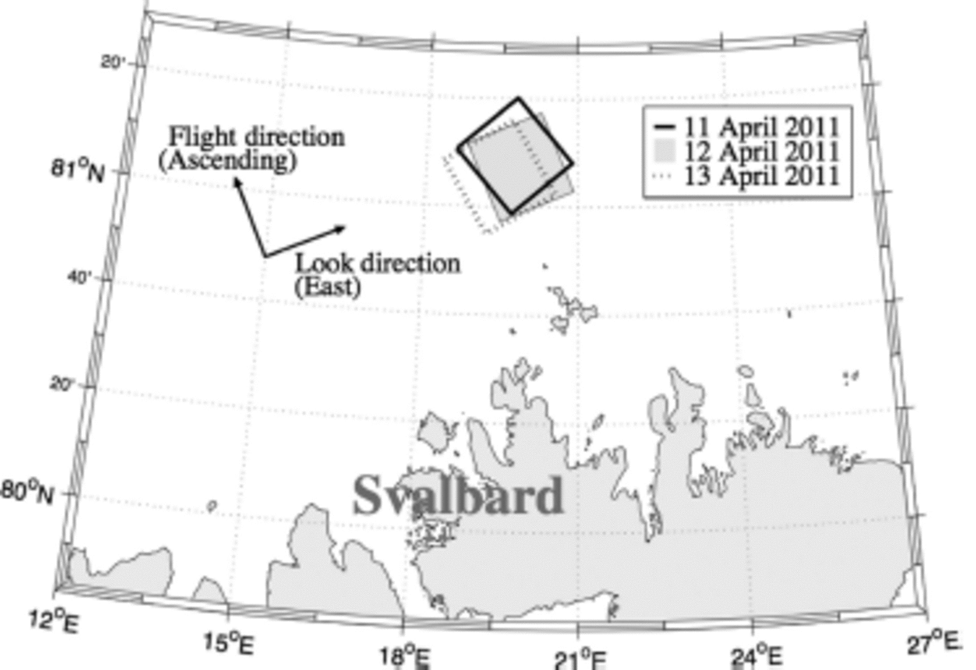
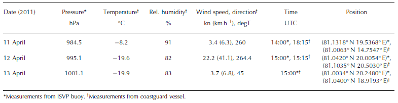
This study is based on three fine quad-pol satellite images acquired by the Canadian C-band SAR satellite, RADAR-SAT-2. The scenes are located north of Svalbard (Fig. 1) and were obtained on three consecutive days during April 2011. The entire scenes, not just the intersection, are utilized in the following analysis. Acquisition time, position, incidence angle and resolutions for each scene are given in Table 1 . The study area comprises first-year drifting sea ice at various stages of development and open and refrozen leads (Reference Renner, Hendricks, Gerland, Beckers, Haas and KrumpenRenner and others, 2013). In situ observations were collected from the bridge of the Norwegian coastguard vessel Svalbard and an Iridium Surface Velocity Profiler (ISVP) buoy deployed on an ice floe. Coincident observations, from 11–13 April 2011, are listed in Table 2 . The distance between the centre point of the respective scene and the vessel was 82, 11 and 19 km on 1 1, 12 and 13 April, respectively. On 12 April the ship was within the scene.

Fig. 1.

Locations of the RADARSAT-2 images.

Table 1.

Information about the satellite scenes. CIA is the centre incidence angle. IACF is the incidence-angle correction factor. The resolutions are ground resolutions and the numbers in parentheses are the resolution after the averaging operation in Eqn (2)

The scene acquired on 12 April 2011 coincides with various in situ data, such as helicopter-borne thickness measurements, positions from different GPS trackers, a bridge-based sea-ice observation log of the sea-ice conditions and optical photographs. Further details regarding this scene are described by Reference MoenMoen and others (2013). No precipitation was observed between the acquisition times of the first and the last scene.

The polarimetric intensity channel combinations, |HH-VV|, 2|HV| and |HH+VV|, are assigned to the red, green and blue channels, respectively (Fig. 2), to produce what is commonly known as a Pauli image (Reference Lee and PottierLee and Pottier, 2009). The satellite scenes are provided in slant range, thus the width of the Pauli images varies due to different incidence angles. The images are ∼28 km across on the ground. The geographical overlap of the scenes is good (Fig. 1), but ice drift causes problems when comparing multiple SAR scenes. Some structures in the ice cover are recognizable in two or more of the Pauli images. Examples of structures that may be traced by visual inspection are indicated by the arrows in Figure 2.

Fig. 2.

Pauli images of the three scenes (11-13 April 2011, left to right) and examples of visually identified matching structures. The images are shown in slant range geometry and are ∼28 km across on the ground.

In compacted pack ice and freezing conditions, the most deformed and thickest ice classes are expected to remain stable on a daily or shorter timescale under stable atmospheric conditions. Thus, their SAR signatures are expected to remain largely unchanged. Given the low air temperature (Table 2), the thin-ice and open-water classes are likely to change the most due to new ice formation. Wind can substantially alter the ice cover, due to increased dynamics leading to deformation and opening of leads. The latter then provides areas for new ice formation. The study area was dominated by compacted pack ice with very little open water, reducing the freedom of ice movement. However, the substantial variation in wind speed and direction (Table 2) suggests that both divergent and convergent ice motion took place between acquisition of the first and last SAR scenes. We also find evidence of such ice motion in the Pauli images of 11 and 12 April 2011; the images indicate the opening of a lead between the two image acquisitions. In the following we refer to the scenes acquired on 1 1, 12 and 13 April 2011 as S11, S12 and S13, respectively.

Table 2.

Information about collected in situ data: barometric pressure; air temperature; relative humidity; wind speed and wind direction. The wind direction is in degrees true north (degT)

Methods

Radiometric correction

Radiometric correction of remotely sensed data involves calibration of the digital images to improve the consistency of the backscatter magnitudes across different incidence angles. The sensor-specific backscatter generally decreases with increasing incidence angle (Reference OnstottOnstott, 1992; Reference GillGill and Yackel, 2012; Reference Gupta, Barber and IsleifsonGupta and others, 2014). Thus, it is essential that such incidence-angle effects are taken into account prior to quantitative image analysis to ensure comparability between multiple datasets. In this study, we performed a radiometric correction on the complex scattering coefficients in all channels. The coefficients used in this study are standard sigma0 calibrated single-look complex (SLC) matrices, as output from the PolSARpro v.4.2 software (Polarimetric SAR data processing and educational toolbox; Reference PottierPottier and others, 2009; Reference Pottier and FamilPottier and Ferro-Famil, 2012). The scattering coefficients are subscripted with the associated receive-and-transmit polarization. The scattering vector, which in our case is from linear full-polarimetric data, is given by s = [SHH, 12 (SHV + SVH),S V V ], where we assume reciprocity (SHV — SVH). The operator () defines the ordinary transpose operation, and the factor 1 j 2 ensures that the averaged cross-pol term preserves the power contained in the individual original cross-pol terms. The radiometrically corrected scattering vector, s_rc, is obtained from the uncorrected scattering vector, s, by multiplying the square root of the sine ratio of the centre incidence angle of the image to be corrected, 6 , and a reference incidence angle, θ_ref

(Reference SunSun and others, 2002):

(1)

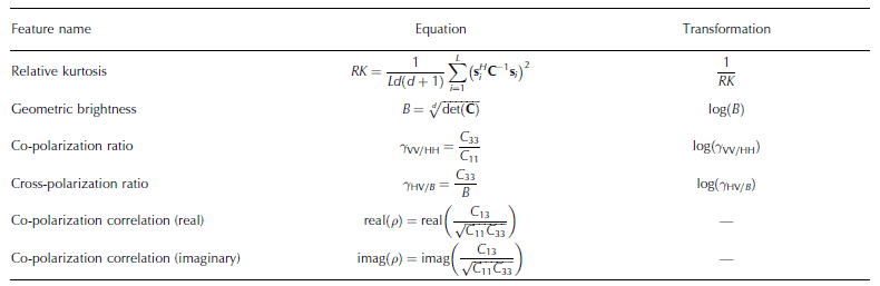
We perform the correction directly on the scattering vectors, not the intensities, hence we include the square root. This type of correction only affects the brightness feature (Table 3), as it is divided away in all the other features.

In this study all scenes are corrected to reference angle, θ_ref = 40.0°, which is the centre incidence angle of the reference.

The square-root factor (incidence-angle correction factor, IACF) for each scene is shown in Table 1. By correcting all range lines of each image by the same amount, using a fixed 6, we introduce an error, because strictly speaking 6 should vary across each image. The scenes are ∼28 km in ground range, and the largest angular width is 1.9°. The error introduced by this approximation is <2% across the range, which we find acceptable given the class brightness variability.

Table 3.

Features from the extended polarimetric feature space (EPFS) method. The transformations to make the features Gaussian-like are listed in the right column. L is the number of pixels in the stepping window, d is the dimension of the scattering vectors. s and C are the scattering vector and the polarimetric covariance matrix, respectively. C_ij is the C-matrix entry of row i and column j

Automatic segmentation

We calculate the polarimetric covariance matrix, C, by averaging over L = 21 x 21 = 441 pixels, each represented by a radiometrically corrected scattering vector, s, defined above. The averaging is done with a stepping window:

(2)

The operator ()^H defines the Hermitian transpose operator. From the polarimetric covariance matrix and the radio-metrically corrected scattering vectors we calculate six features using the extended polarimetric feature space (EPFS) method (Reference Doulgeris and EltoftDoulgeris and Eltoft, 2010; Reference Doulgeris and OuwehandDoulgeris, 2013). Five of these features are basic polarimetric parameters that have been used in many similar studies. The sixth, the relative kurtosis, is a statistical measure of the shape of the intensity distribution. The names and equations of the features are shown in Table 3. (More information about the features and their interpretation with respect to sea ice is given by Reference MoenMoen and others (2013).) Using simple transformations on all elements in the extracted feature vector set (Table 3) we can make them more Gaussian-like, i.e. the probability density functions (PDFs) are nearly symmetric and have Gaussian bell shapes. This enables the use of a simple yet efficient algorithm, i.e. the mixture-of-Gaussians segmentation algorithm, which makes it suited for operational use.

The segmentation algorithm divides and smooths the satellite image into a predefined number of classes. We constrain the algorithm to find seven classes; the reasoning for this is explained in the following subsection. The algorithm will always split the worst-fitted class first, hence we minimize the total fitted error. Contextual smoothing is an image-smoothing approach which considers the labels of the neighbouring pixels in the labelling of a given pixel. The smoothing process makes the segmentation less speckled and thus easier to interpret. Feature extraction, the automatic segmentation algorithm and contextual smoothing are explained in more detail by Reference Doulgeris and EltoftDoulgeris and Eltoft (2010), Reference Doulgeris and OuwehandDoulgeris (2013) and Reference MoenMoen and others (2013). In the following we assume that the same classes are present in all three scenes.

Reference

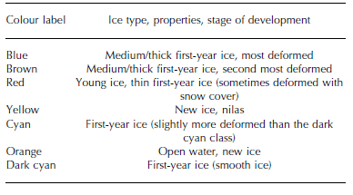
The S12 scene is chosen as the reference because of its accompanying in situ data. Reference MoenMoen and others (2013) segmented the scene into five classes, but they revealed one class to be bimodal (mixed) and therefore suggested increasing the number of classes. In this study, we have used the same algorithm and increased the number of classes to seven. This was necessary to obtain classes with smooth and unimodal histograms for all features. Each class was labelled using suitable ancillary data and the expert knowledge described by Reference MoenMoen and others (2013). The ice experts were able to label only four ice classes, so labelling seven classes was not trivial. Although the classes are not visually distinguishable in photographs, Pauli images, etc., they are statistically distinguishable using the polarimetric data. In this study the remaining three classes were labelled using statistical analysis of polarimetric features, together with a physical interpretation of these features. The class labels and associated ice types are given in Table 4. The ice types are based on WMO stage-of-development definitions (CIS, 2005).

Table 4.

Class labels and associated ice types. The colours refer to those in the segmentations (Fig. 3)

Manual matching and automatic labelling

After segmentation, S11 and S13 were manually labelled by matching them visually to the classification of the S12 scene and by comparing the segmentations and Pauli images. Using the same segmented scenes as for the manual matching, we used statistical Gaussian distance measures to automatically label classes. This test was performed to check whether a particular distance measure was preferable when labelling the unknown classes. The transformation of the features (Table 3) justifies the use of Gaussian distance measures. Three different distance measures based on mean values and/or covariance matrices from multivariate Gaussian distributions (Eqns (3-5)) were tested on the assumed multivariate Gaussian feature vector. They are all straightforward calculations and hence suited for operational use. In addition we tested the Kullback-Leibler distance (Eqn (6)) derived under the complex Wishart model (Reference GoodmanGoodman, 1963). It has a simple mathematical form and uses the complete information contained in the polarimetric covariance matrices (Eqn (6)), which is why we also test it. Ni and Nj are two normal distributions with means μ _i and μ _j and covariance matrices Σ _i and Σ _j , respectively. Σ is the mean of Σ _i and Σ _j . kΣ is the dimension of Σ and is equal to 6. Ci and Cj are the polarimetric covariance matrices for class i and j, respectively. kC is the dimension of C and is equal to 3. The operator tr defines the trace of a matrix, () is the inverse and () is the transpose operation.

Mahalanobis distance (Reference Theodoridis and KoutroumbasTheodoridis and Koutroumbas, 2009)

(3)

Multivariate Gaussian Bhattasharyya distance (Reference Theodoridis and KoutroumbasTheodoridis and Koutroumbas, 2009)

(4)

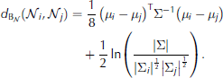
Multivariate Gaussian Kullback–Leibler distance (Reference HersheyHershey and Olsen, 2007)

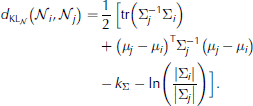
Symmetric multivariate Gaussian Kullback–Leibler distance

(5)

Complex-Wishart Kullback–Leibler distance (Reference FreryFrery and others, 2014)

(6)

The manually matched images of S11 and S13 (Fig. 3a and c) were used to evaluate the automatic labelling because, ideally, the results based on the same scene should match. The same automatic labelling procedure was applied for each distance measure. A 7 x 7 distance matrix, with each column representing the unknown test class and each row corresponding to a class in the reference data, was used to identify the nearest classes. We used a sequential approach, taking the best match first, i.e. the test class corresponding to the minimum distance was assigned to the corresponding reference class. The corresponding row and column were removed and the row and column of the new minimum distance were located. This step was repeated until all classes were labelled.

Results

Manual matching and automatic labelling

The manually matched labels are shown in Figure 3. The colours of the segmented image are chosen arbitrarily to be visually distinct and do not represent WMO colour coding. In the following, it is important to note that (1) the S11 and S13 scenes only partly overlap with the reference scene and (2) the images have different ground resolutions. The S12 and S13 scenes look consistent, the main structures are recognizable and have the same labels in both images. The 511 scene appears substantially different, so its labels do not easily match those of the S12 scene. Only a few structures are recognizable and have the same label in the S11 and 512 images (e.g. areas indicated by white arrows in the Pauli images (Fig. 2)).

Fig. 3.

Automatically segmented, manually matched results for 11-13 April 2011, left to right. See Table 4 for labels. The manually matched images of 11 and 13 April 2011 were used to evaluate the automatic labelling. The images are shown in slant range and represent ∼28km across on the ground.

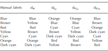
Table 5 shows the results of automatic labelling of the automatic segmentation of the S11 scene, together with the manually matched labels. The automatic labelling of the S11 scene performed by the Mahalanobis distance, d _M, agrees best with the manual matching: all classes match except the yellow and brown ones. The labelling result calculated from the Bhattasharyya distance, d _BN, has no classes equal to the manual matching.

Table 5.

The manually matched labels and the corresponding automatic labelling of the automatic segmentation of 11 April 2011. dM is the Mahalanobis distance, dBN is the multivariate Gaussian Bhattasharyya distance, dKLN is the multivariate Gaussian Kullback–Leibler distance and dKLW is the complex Wishart Kullback–Leibler distance

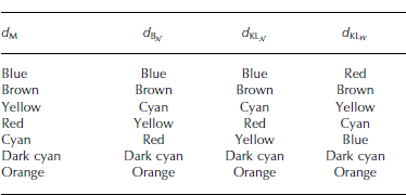
The automatic labelling of the S13 image is identical to the manual matching (Fig. 3) for all distance measures, but the distance priority in which the classes are assigned is different for each distance measure (Table 6). The manually matched blue class of the S13 image and the blue class in the reference data are the nearest classes in all distance measures, except for the complex Wishart Kullback–Leibler distance (Eqn (6); Table 6). This is not surprising given the totally different data domain of that measure.

Table 6.

The automatic labelling of the automatic segmentation of 13 April 2011. Each column represents the order in which the classes were assigned by the distance measures. d _M is the Mahalanobis distance, d _BN is the multivariate Gaussian Bhattasharyya distance, d _KLN is the multivariate Gaussian Kullback– Leibler distance and d _KLW is the complex Wishart Kullback–Leibler distance

Supervised classification

The results of the supervised classification are shown in Figure 4. Few similar structures (e.g. those indicated in Fig. 2) are recognizable from the two supervised classified scenes. The structures in the supervised classification of the S11 scene do not resemble those in the Pauli image nor those in the automatic segmentation. The new ice/nilas (yellow) dominates, followed by the most deformed first-year ice (blue, Table 4).

Fig. 4.

Supervised classifications of the 11 and 13 April 2011 scenes, using the S12 scene (Fig. 3b) for reference. The colours correspond to those in Figure 3. The labels are given in Table 4. The images are shown in slant range and are ∼28 km across on the ground.

Contrarily, the supervised classification of the S13 scene contains similar structures to those in the Pauli image and the automatic segmentation and appears to be reasonable, but not exactly the same. The most notable difference compared with the automatic labelling is that the open water/new ice (orange) is absorbed into the new ice/nilas (yellow) and the number of pixels in the second most deformed first-year ice (brown) increases at the expense of several other classes.

Discussion

Prior to all segmentations and classifications, we made assumptions regarding the ice conditions: the same classes are present in all three scenes, no new classes evolved and no classes disappeared. However, the predefined seven classes may develop into other existing classes (e.g. open water can freeze and become new ice, smooth ice can be exposed to rafting and become more deformed, the ice pack can break up and create open leads). Considering the prevailing weather conditions, we find this a reasonable assumption because our selection of classes should cover the listed potential changes. However, in general, this assumption does not hold and must be considered when implementing an operational algorithm. Wet snow, slush and flooding of the ice are changes that will weaken our assumption, as these changes are known to affect the backscattering and are not covered in any of our ice classes. Multi-year ice is also known to have a different scattering signature to other ice types. We have not included the aforementioned classes as they were not present in any of our scenes.

Our study here is limited in time and space, using only three scenes acquired within 3 days. Looking over a different timescale and/or into a different region will involve adjusting the number and composition of the selected classes; this is a challenge for the future.

In contrast to the manual matching of the S13 scene, the manual matching of the S11 scene was difficult, possibly due to the few visually identifiable structures in both the image and the reference scene (Fig. 2). However, some manually matched classes, such as the smooth first-year ice (dark cyan), new ice/nilas (yellow) and open water/new ice (orange), should be fairly well matched (corresponding areas marked by the white arrows in Fig. 2 are labelled the same colour in Fig. 3).

Our results show that automatic segmentation and labelling works quite well for S13, but poorly for S11. All distance measures agree on the (automatic) labelling of S13; none agree for S11. Even though the automatic labelling and the manual matching agree to some extent, it is not necessarily the correct labelling. One disadvantage of the automatic labelling procedure is that there will always be a nearest class, which does not necessarily correspond to the manual matching. This will be the case if, for instance, the class properties have evolved and/or the desired classes of the actual image are not represented in the reference image. The polarimetric features are not expected to be stable through the seasonal cycle. How each class property changes with feature, incidence angle, season and area will be highly relevant in future studies.

The automatic segmentation is based on numerical values from each scene individually, while the supervised classification works pixel-wise, based on values transferred from the reference scene. If the statistics between the three days were unchanged, the automatic labelling and the supervised classification of the same days would be identical. They are evidently not, because the statistics have changed.

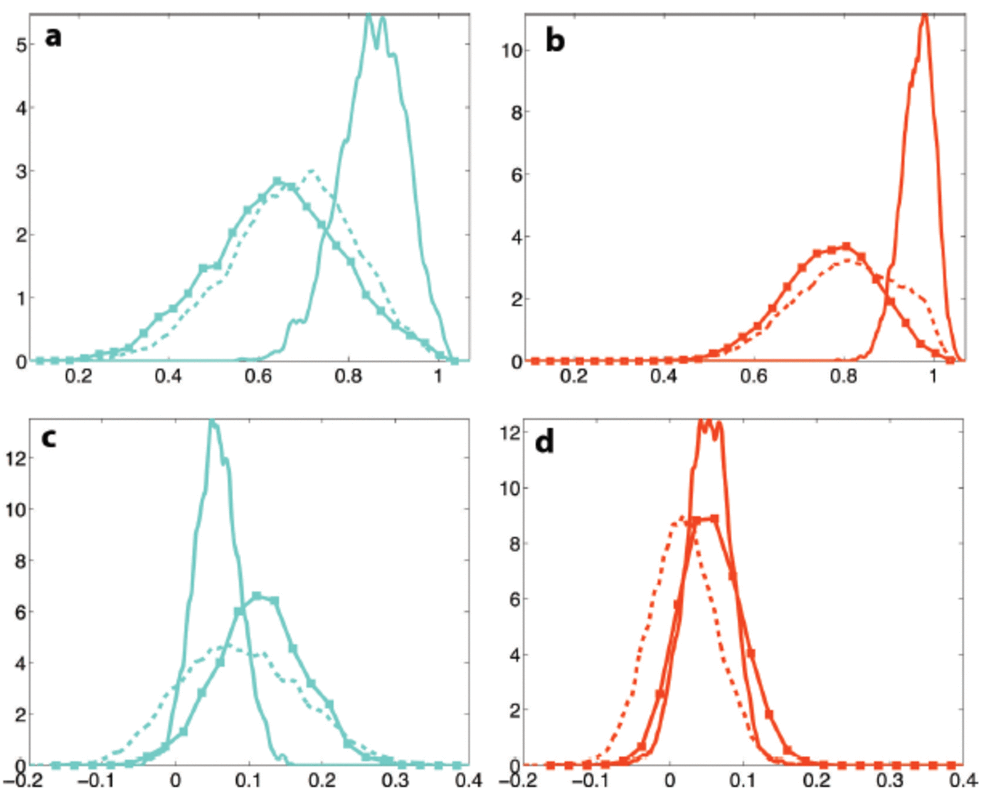
The S11 scene is obviously problematic. This is supported by the PDFs of each class and each feature. Figure 5 shows two classes from S12 and S13 that are quite well aligned, whereas the classes from S11 are shifted. The same is also true for other classes from the S11 scene. We see that statistical class properties (mean value and variance) change differently with different features and incidence angles (Fig. 5 and 6). This could be one reason for the disagreement of the automatic labelling of S11.

Fig. 5.

Examples of probability distributions for the relative kurtosis (a, b) and the imag(p) (c, d) features. The left column (a, c) represents the cyan class, and the right column (b, d) is the red class. The solid curves represent 11 April, the dashed curves 12 April and the solid curves with squares 13 April, all from 2011.

Fig. 6.

Examples of probability distributions for the log brightness feature. The top row (a–c) shows the brightness not radiometrically corrected. The bottom row (d–f) shows the radiometrically corrected brightness feature. The left column (a, d) represents the cyan class, the middle column (b, e) is the red class and the right column (c, f) is the blue class. The solid curves represent 11 April, the dashed curves 12 April and the solid curves with squares 13 April, all from 2011.

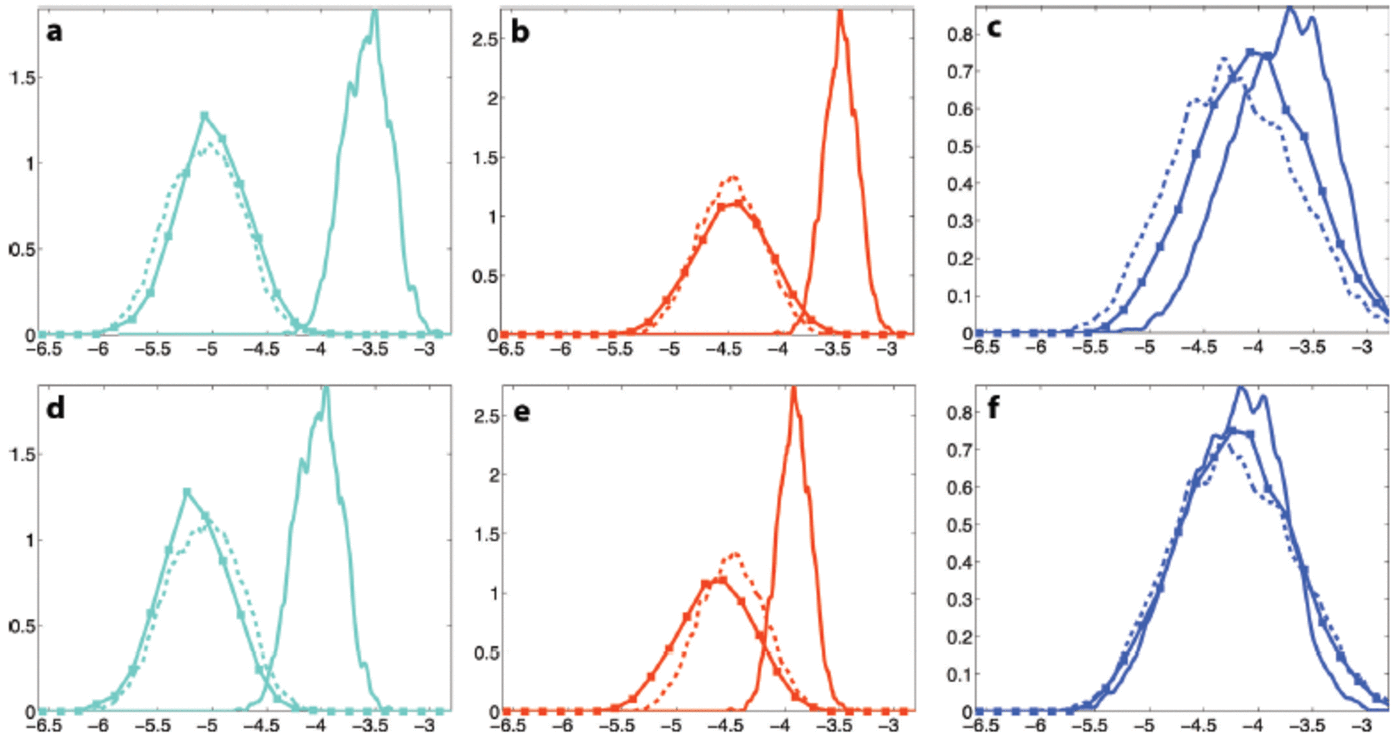
Incidence-angle correction (radiometric correction) adjusted the misalignment to some extent for some classes. Recall that this type of correction only affects the brightness feature. Figure 6 illustrates three different effects of the radiometric correction. For three of the seven classes the correction made the alignment between S12 and S13 worse (e.g. the young ice class (red); Fig. 6b and e). However, the shift is not significant with respect to the class variation. Our results show that the performance of the automatic labelling and the supervised classification of S13 using corrected data are very good (Fig. 3c; Table 6). The correction did not make any substantial difference for the second smoothest first-year ice (cyan) of S13 (e.g. Fig. 6a and d), i.e. the PDF is shifted a small amount to the right, but the overlap with the S12 PDF stays approximately the same. For two classes, most deformed (blue) and smooth first-year ice (dark cyan) the correction of S13 was very good (Fig. 6c and d). As seen in Figure 6, the S11 most deformed ice (blue) is also very well aligned with the reference data. This is the only class in the S11 image that is well aligned with the reference class after correction. In the S11 image the radiometric correction improves the alignment of five of the seven classes (e.g. Fig. 6b and e, 6a and d). However, the improvement is not sufficient to make the automatic labelling and the supervised classification work. The second most deformed first-year ice (brown) in the S11 image shows no difference in overlap before and after correction, similar to the results of the S13 cyan class shown in Figure 6a and d.

Incidence-angle correction (radiometric correction) adjusted the misalignment to some extent for some classes. Recall that this type of correction only affects the brightness feature. Figure 6 illustrates three different effects of the radiometric correction. For three of the seven classes the correction made the alignment between S12 and S13 worse (e.g. the young ice class (red); Fig. 6b and e). However, the shift is not significant with respect to the class variation. Our results show that the performance of the automatic labelling and the supervised classification of S13 using corrected data are very good (Fig. 3c; Table 6). The correction did not make any substantial difference for the second smoothest first-year ice (cyan) of S13 (e.g. Fig. 6a and d), i.e. the PDF is shifted a small amount to the right, but the overlap with the S12 PDF stays approximately the same. For two classes, most deformed (blue) and smooth first-year ice (dark cyan) the correction of S13 was very good (Fig. 6c and d). As seen in Figure 6, the S11 most deformed ice (blue) is also very well aligned with the reference data. This is the only class in the S11 image that is well aligned with the reference class after correction. In the S11 image the radiometric correction improves the alignment of five of the seven classes (e.g. Fig. 6b and e, 6a and d). However, the improvement is not sufficient to make the automatic labelling and the supervised classification work. The second most deformed first-year ice (brown) in the S11 image shows no difference in overlap before and after correction, similar to the results of the S13 cyan class shown in Figure 6a and d.

Our results show that the performed radiometric correction is not sufficient when the incidence-angle difference between scenes is large, and examples show that even with similar incidence angles, the correction can worsen the alignment of some PDFs. However, we conclude that the advantages of performing the correction are greater than the disadvantages.

A good incidence-angle correction is essential for consistent results using data covering the same area, but with different incidence angles. To improve the correction may require correcting differently for each channel and/or (more problematic) each class. This is an important future research topic. However, total compensation for the incidence angle will be impossible, as it varies with ice type (Reference Makynen, Manninen and SimilaMakynen and others, 2002) and possibly also with polarization.

The three scenes have different incidence angles, and thus different ground resolutions. In our study we have averaged the scenes by the same amount. The consequence is that the smoothing level on the ground is different in each scene; ice structures clearly visible in one scene may not appear in another scene. Preliminary results indicate that adjusting the amount of averaging such that the ground resolution is similar in all scenes improves the alignment of the PDFs for each class (e.g. Fig. 5 and 6).

It is possible that the incidence angle of the S11 scene is too different to be corrected according to the centre incidence angle and compared with the reference scene. Applying the correction per range line was thought to give only slight improvements, but this needs to be confirmed in future studies.

The wind speed on 12 April 2011 was very high, compared with the other days (Table 2). This will most likely affect two main processes: the ridging of sea ice, leading to increased deformation, and the opening of leads. The latter, combined with the low air temperature, may cause formation of new smooth ice (e.g. nilas, grey ice). We have seen that the open-water/new-ice (orange) class almost disappears in the supervised classification of the S13 scene (Fig. 4). The explanation could be that the open water/new ice (orange) from S12 has evolved and become frozen, i.e. new ice/nilas (yellow). In situ measurements from 12 April 2011 indicate that leads may freeze quite fast. In Figure 3 the proportion of deformed ice/ridges (blue) is larger in the S11 than the S12 image, but the amount of new ice/nilas (yellow) is approximately the same. The supervised classification (Fig. 4) indicates a lot more both new ice/nilas (yellow) and deformed ice/ridges (blue) in the S11 than the S12 image. According to the weather conditions we would expect more deformed ice and opening of leads in the S12 image than the S13 image. We do not believe that the problems regarding the S11 scene are related to evolution of ice classes; they are more likely to be due to incidence-angle effects.

Conclusion

At present, no automatic methods for classification of radar images of sea ice are robust enough to be used throughout the year. We have investigated two methods for classification of polarimetric radar images of sea ice. The algorithms were assessed in terms of their ability to produce consistent results under varying environmental conditions and viewing geometry. The presented work is limited both in time and space, hence definite conclusions are not possible.

We have shown that automatic segmentation looks reasonable for all three scenes individually. The main structures are recognizable in both the Pauli (Fig. 2) and the segmented image (Fig. 3). However, when we attempt to use the S12 image as reference data to label the unknown classes of the test scenes, S11 and S13, the results differ. The manually matched labels and the automatic labelling are identical for all distance measures tested for the S13 image. For the S11 scene none of the distance measures used for automatic labelling harmonize completely with the manually matched labels. The Mahalanobis distance is the best-performing distance measure. It matches the labels of the S13 image perfectly, and five of seven labels of the S11 image.

The supervised classification is reasonable for S13, but very poor for S11. We suggest the problem with the S11 scene is mainly related to incidence-angle effects (e.g. brightness and resolution).

The two test scenes were radiometrically corrected to the centre incidence angle of the reference data, but the correction of the S11 scene does not fully account for the differences. The radiometric corrections are just a first-order approximation, but we conclude that the advantages of performing the correction are greater than the disadvantages. A good incidence-angle correction is essential for comparing scenes acquired at different angles, but as our dataset is not suitable for such an investigation we leave this for future studies. However, we suggest that an improved incidence-angle correction could be accomplished by correcting each channel, or even each class, independently. The latter is supported by our study. The performed incidence-angle correction affects the classes differently (Fig. 6). Yet, correcting each class individually is obviously impossible without a priori information on the corresponding ice types.

In this study we had to assume that the classes did not change between the scenes. The number of classes in each scene is an important issue. Future research should try to automatically determine the number of classes. Other relevant topics in future studies are how sea-ice class properties change with feature, area, etc.

Under similar incidence-angle conditions the proposed automatic labelling method gives reasonable results and has the potential to be developed into an operational algorithm. However, the presented results are only valid for winter conditions. Preliminary analysis, i.e. supervised classification, of three other overlapping scenes from the same period and area gives results similar to the S13 supervised classification. Structures clearly recognizable in the Pauli images are also visible in the supervised classifications. The centre incidence angles are in the range 30–45° and the weather conditions appear reasonably stable (<5°C).