II. THE MULTI-SOURCES SYSTEM

To illustrate how WPT works, a receiver is placed in different configurations at a given distance with a given orientation, above a conventional flat transmitter represented by a single turn coil.

The effect of receiver's disposition on the WPT efficiency is expressed by the coupling factor of which the value describes the amount of energy transferred from a transmitter toward a receiver:

(1) $$k = \displaystyle{{\emptyset _r} \over {\emptyset _t}} = \displaystyle{{n_r} \over {n_t}} \displaystyle{\zsint B_r cos(\theta _r ) \cdot \partial A_r \over \zsint B_t \cdot \partial A_t}, $$

where B _r is the received magnetic flux density at a given point across the receiver area; θ _r is the receiver orientation angle; n _r the number of turns at the receiver; A _r the receiver cross-sectional area. Terms with the subscripts “t” correspond to the transmitter side.

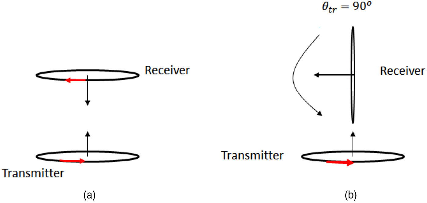
Figure 1(a) shows a conventional system where both transmitter and receiver have similar areas and are placed close to each other. Such a configuration provides a magnetic flux density more or less constant over A _r and the magnetic field lines are parallel to the receiver's axis. Consequently, equation (1) becomes

(2) $$k_1 = \displaystyle{{n_r} \over {n_t}} \displaystyle{\zsint {B_r \cdot \partial A_r} \over \zsint {B_t \cdot \partial A_t}}. $$

Fig. 1.

(a) Conventional receiver disposition, (b) our receiver disposition.

By applying equation (1) to the configuration presented in Fig. 1(b) the coupling factor becomes:

(3) $$k_1 = \displaystyle{{\emptyset _r} \over {\emptyset _t}} = \displaystyle{{n_r} \over {n_t}} \displaystyle{\zsint {B_r cos(90^\circ ) \cdot \partial A_r} \over \zsint {B_t \cdot \partial A_t}} = 0.$$

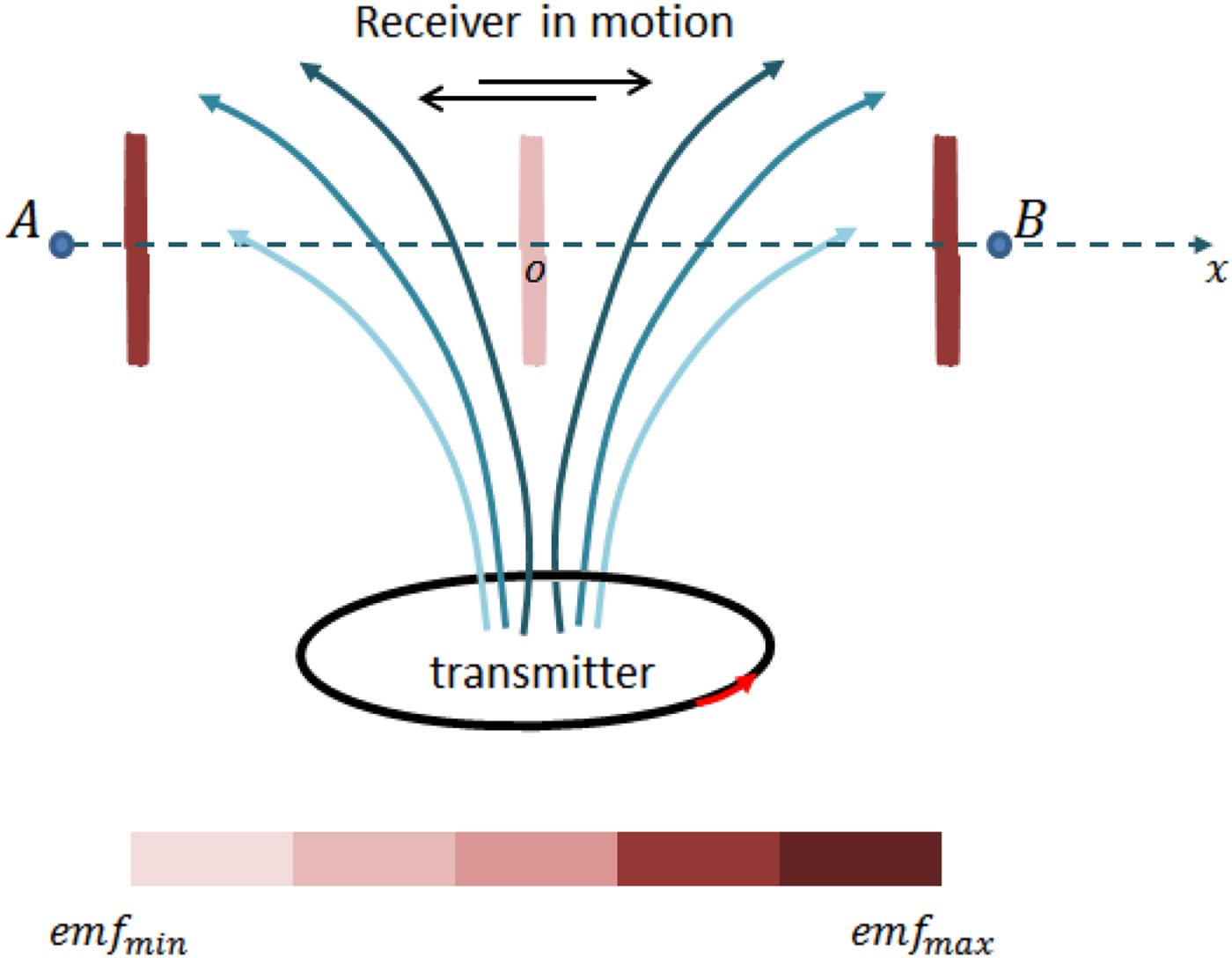
In other words, the receiver's does not collect any field line and there will be no power transferred to the receiver. The comparative study in [Reference Waffenschmidtt and Staring9] shows how the area difference between the transmitter and the receiver as well as the distance separating them affects the coupling factor value. For this purpose, the authors have considered concentric and flat coils for both transmitter and receiver. However, as soon as the receiver starts moving as in [Reference Ye, Yan, Wang and Ma12], the leakage field intensity increases and the magnetic flux density becomes a function of the x-coordinate.

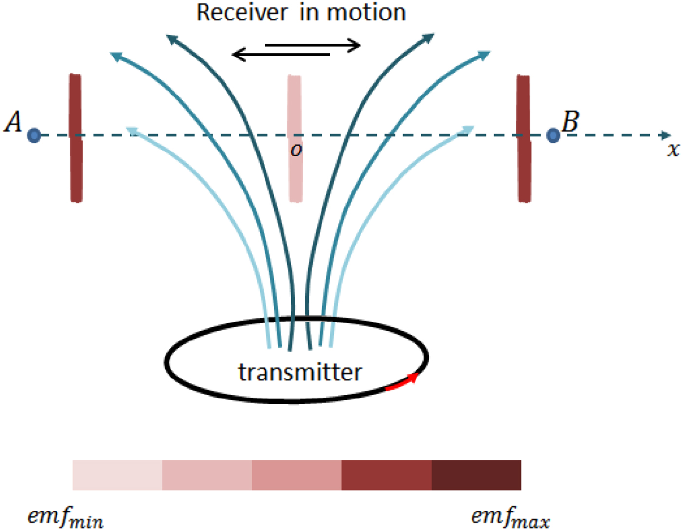
Figure 2 shows a rough distribution of magnetic field lines between two points A and B and where a receiver similar to the one in [Reference Ye, Yan, Wang and Ma12] is moving back and forth. It can be observed that the induced emf varies according to the receiver's position and decreases each time the receiver approaches the center “o”. The coupling factor expression becomes:

(4) $$k_3 = \displaystyle{{n_1} \over {n_t}} \displaystyle{\zsint {B(x) \cdot cos(\theta _r ) \cdot \partial A_r} \over \zsint {B_t \cdot \partial A_t}} \ll k_3. $$

Fig. 2.

Magnetic field lines along a non-parallel oriented path.

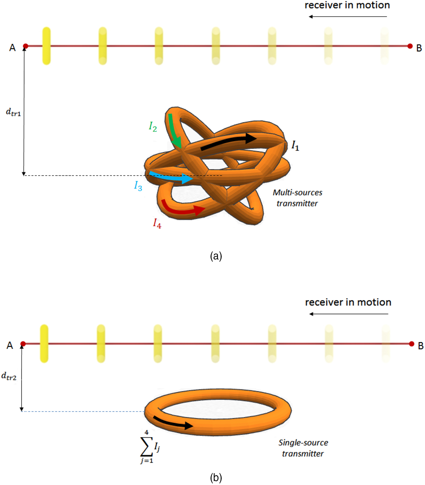
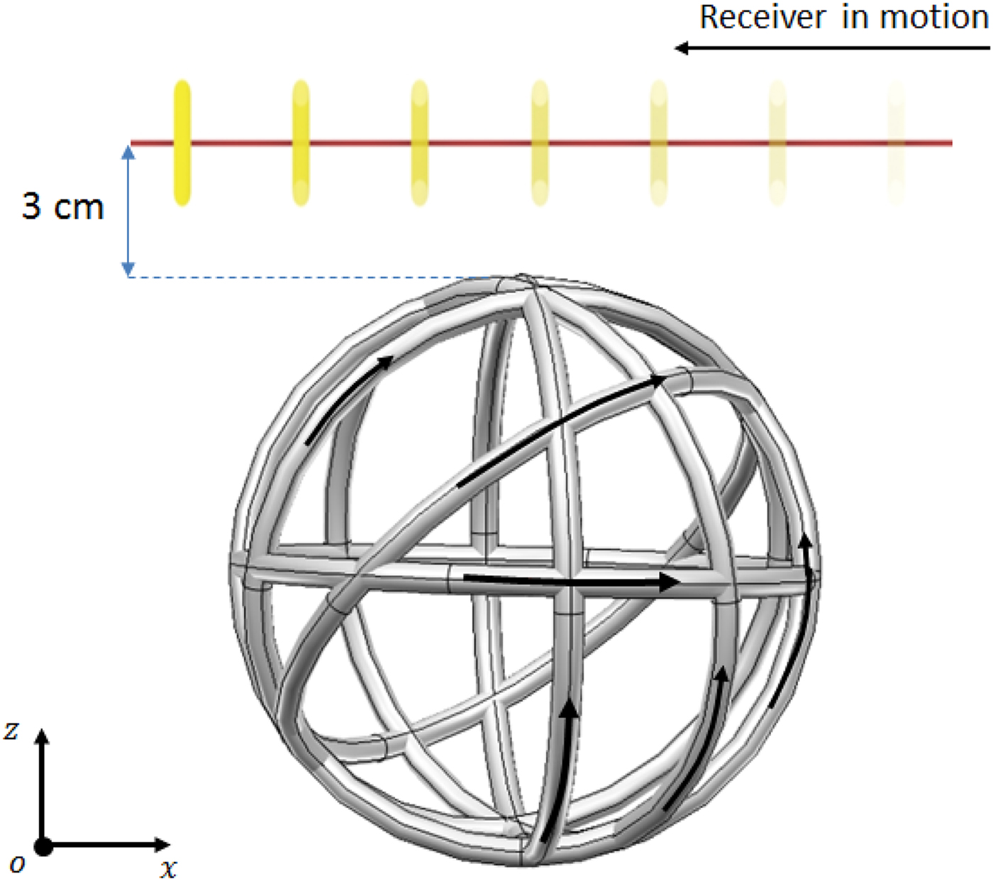
The WPT system studied in this paper is dedicated to applications where the shift angle between transmitter and receiver respective axes is constraining. For this purpose, the proposed transmitter topology presented here is shown in Fig. 3. Such a topology allows a more efficient energy re-distribution so that the receiver always sees the same magnetic flux.

Fig. 3.

(a) Receiver in motion above a concentric multi-source transmitter, (b) receiver in motion above a conventional transmitter.

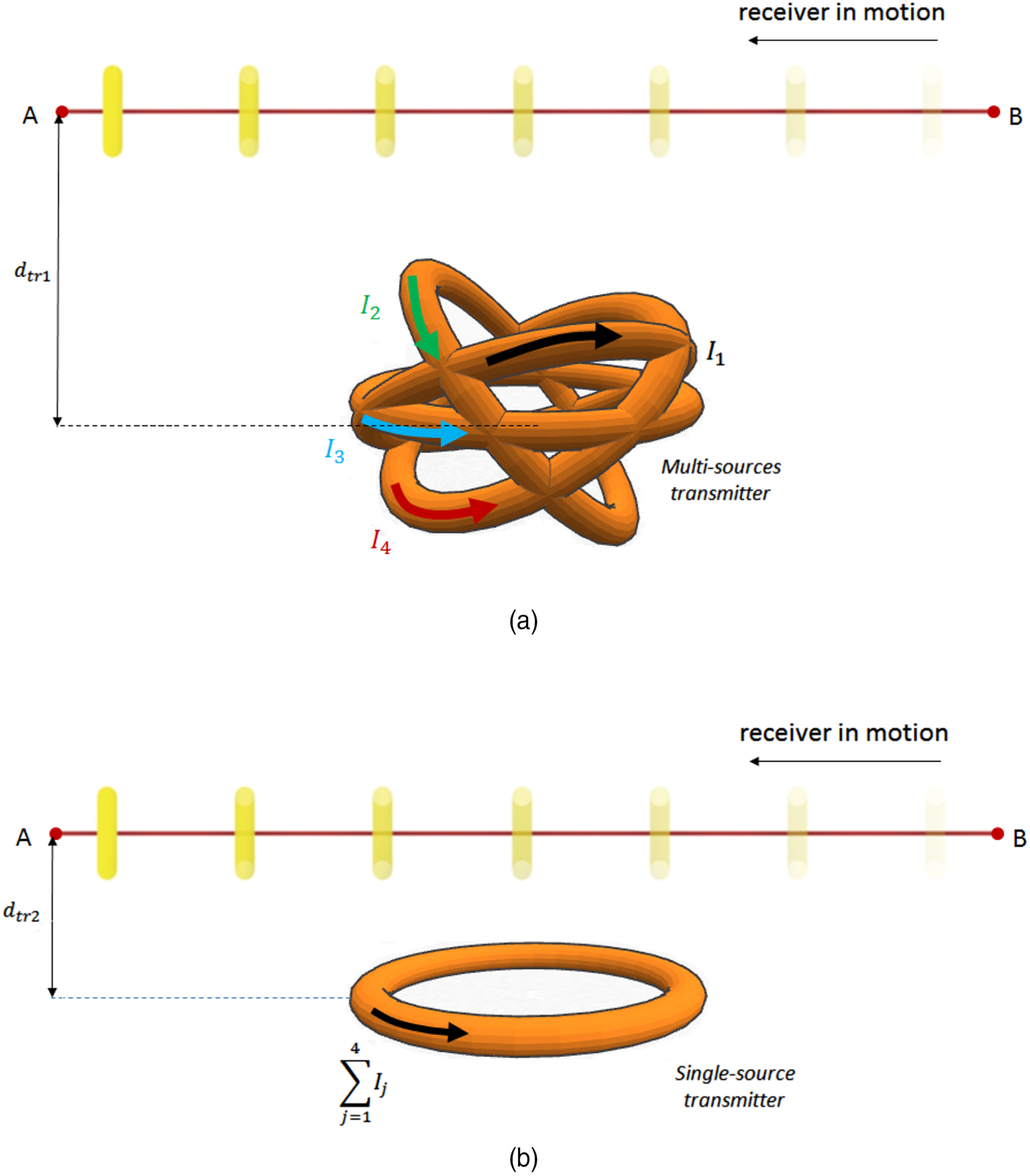
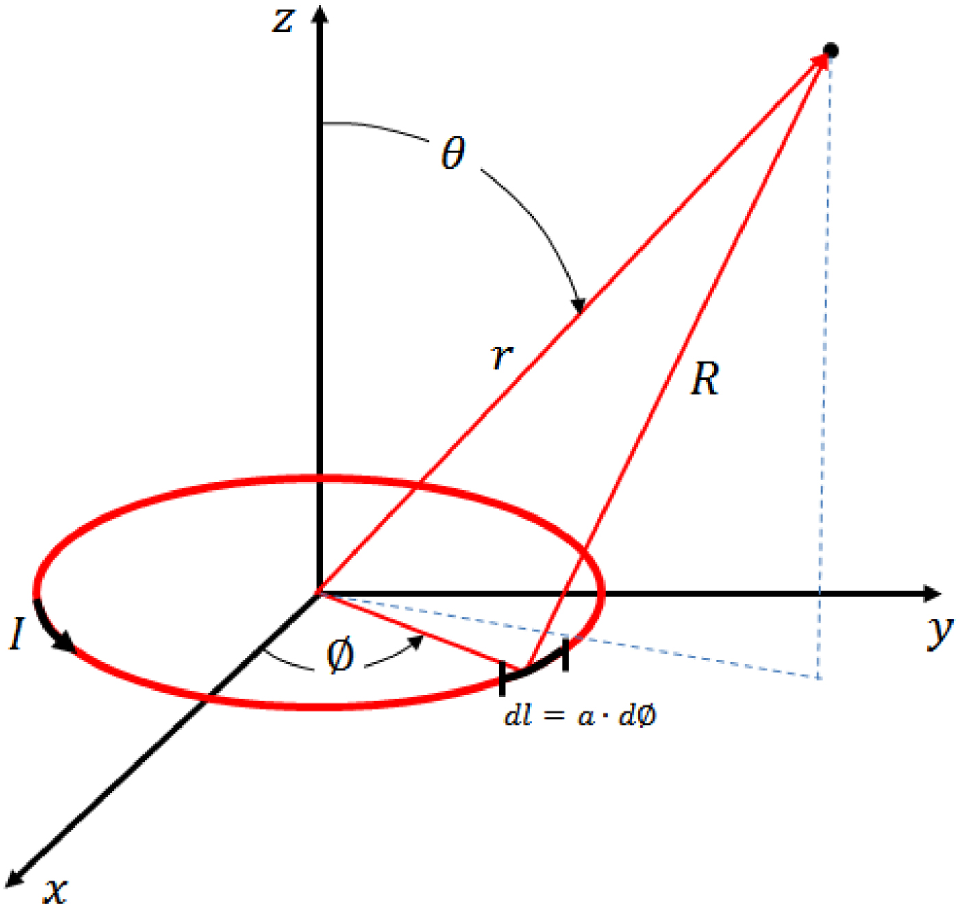
The transmitter-to-receiver distance of the multi-source transmitter $d_{tr_1} $ is expressed as following: $d_{tr_1} = d_{tr_2} + max(r_i \cdot sin(\theta _i ))$ ; where r _i is the source i radius; $d_{tr_2} $ is the transmitter-to-receiver distance of a conventional transmitter;θ _i is the source i spherical orientation angle shown in Fig. 4. For the design of such systems, the inverse problem widely used in electromagnetic characterization is solved. This gives the sources currents needed to provide the required magnetic field value along the receiver's path (with minimum transmitted energy). Then, obtained systems are compared with the conventional single-source flat transmitters. At this matter, it is worth it to mention that the total current injected in a multi-source transmitter is the same current injected in one conventional transmitter.

Fig. 4.

Magnetic dipole.

III. SYSTEM DESIGN

In this paper, a design methodology for more efficient perpendicular WPT systems is presented. For this purpose an inverse problem-based characterization method is used and where the parameters of each source are obtained by minimizing the error between the total magnetic field emitted by the transmitter in question and the magnetic field needed along the receiver's path. The function describing this error is expressed as follows:

(5) $$\varepsilon (\vec P) = \mathop \sum \limits_{j = 1}^{N_p} \vec H_{mod}^j - \vec H_{def}^j, $$

$\vec H_{mod}^j $ is the magnetic field emitted by the transmitter's model at point J; $\; \vec H_{def}^j $ is the magnetic field defined at point J; $\; \vec P$ is the parameters vector; ε the fitness function representing the minimized error). In order to maximize the coupling factor, the magnetic field component parallel to the receiver's path must be the same along the entire receiver's path. To achieve this, a number of calculation points N _p is considered and along which the fitness function $\varepsilon (\vec P)$ is minimized in terms of the parameters vector $\vec P$ .

A) The characterization method

As stated above, the key point in this work consists of finding a better energy distribution by using different sources rather than one source as it is the case in conventional transmitters. The model used to predict the magnetic field distribution for such a configuration and which assumes a constant current along the source is the magnetic dipole, which is based on Legendre functions:

Thus, the source circumference must remain well below the wavelength (here 2π · a ≤ (λ/20); a is the dipole radius). Thus, the magnetic field emitted by the magnetic dipole “i” at a point “j” along the receiver's path is described as follows [Reference Beghou, Costa and Pichon18]:

(6) $${\vec H}_{mod\;j} ^i = B_{LG \;j}^i \cdot B_{CC \;j}^i \cdot {\vec H}_{cyl\;j} ^i. $$

Where

$$\vec H_{cyl\;j} ^i = \left[ {\matrix{ {\displaystyle{{k \cdot z{ ^{\prime}}_j} \over {4\pi \cdot \rho { ^{\prime}}_j \cdot \sqrt {a \cdot \rho { ^{\prime}}_j}}} \left[ { - L_1 + \displaystyle{{a^2 + \rho { ^{\prime}}_j ^2 + z{ ^{\prime}}_j ^2} \over {\left( {a - \rho { ^{\prime}}_j} \right)^2 + z{ ^{\prime}}_j ^2}} L_2} \right]} \cr 0 \cr {\displaystyle{k \over {4\pi \sqrt {a \cdot \rho { ^{\prime}}_j}}} \left[ {L_1 + \displaystyle{{a^2 - \rho { ^{\prime}}_j ^2 - z{ ^{\prime}}_j ^2} \over {\left( {a - \rho { ^{\prime}}_J} \right)^2 + z{ ^{\prime}}_j ^2}} L_2} \right]} \cr}} \right] \times I^i $$

is the magnetic field in a cylindrical local-coordinates system and where L ₁ and L ₂ are Legendre functions [Reference Abramowitz and Stegun19]. B _LG is the transformation matrix from local to global coordinates system and B _CC is the transformation matrix from cylindrical to Cartesian coordinates and I ⁱ is the current in source i. Then, if we write the magnetic field as:

(7) $$\vec H_{mod\;j} ^i = A_j^i \cdot I^i. $$

With the expression of matrix $A_j^i $ :

$$A_j^i = B_{LG \;j}^i \cdot B_{CC \;j}^i \left[ {\matrix{ {\displaystyle{{k \cdot z{ ^{\prime}}_j} \over {4\pi \cdot \rho { ^{\prime}}_j \sqrt {a \cdot \rho { ^{\prime}}_j}}} \left[ { - L_1 + \displaystyle{{a^2 + \rho { ^{\prime}}_j ^2 + z{ ^{\prime}}_j ^2} \over {\left( {a - \rho { ^{\prime}}_j} \right)^2 + z{ ^{\prime}}_j ^2}} L_2} \right]} \cr 0 \cr {\displaystyle{k \over {4\pi \sqrt {a \cdot \rho { ^{\prime}}_j}}} \left[ {L_1 + \displaystyle{{a^2 - \rho { ^{\prime}}_j ^2 - z{ ^{\prime}}_j ^2} \over {\left( {a - \rho { ^{\prime}}_j} \right)^2 + z{ ^{\prime}}_j ^2}} L_2} \right]} \cr}} \right];$$

and the total magnetic field emitted by the set of N sources at the same point J is expressed as:

(8) $$\vec H_{mod\;j} = \mathop \sum \limits_{i = 1}^N A_j^i \cdot I^i. $$

The magnetic field emitted at P points along the receiver's path becomes then:

(9) $$\vec H_{mod} = \left[ {\vec H_{mod_1} \cdots \vec H_{mod_P}} \right].$$

(10) $$\vec H_{mod} = \left[ {\matrix{ {\mathop \sum \limits_{i = 1}^N \left. {A_1^i} \right \vert _x \cdot I^i} \quad {\mathop \sum \limits_{i = 1}^N \left. {A_2^i} \right \vert _x \cdot I^i \;} \quad { \ldots \mathop \sum \limits_{i = 1}^N \left. {A_P^i} \right \vert _x \cdot I^i} \cr {\mathop \sum \limits_{i = 1}^N \left. {A_1^i} \right \vert _y \cdot I^i \;} \quad {\mathop \sum \limits_{i = 1}^N \left. {A_2^i} \right \vert _y \cdot I^i} \quad { \ldots \mathop \sum \limits_{i = 1}^N \left. {A_P^i} \right \vert _y \cdot I^i} \cr {\mathop \sum \limits_{i = 1}^N \left. {A_1^i} \right \vert _z \cdot I^i} \quad {\mathop \sum \limits_{i = 1}^N \left. {A_2^i} \right \vert _z \cdot I^i} \quad { \ldots \mathop \sum \limits_{i = 1}^N \left. {A_P^i} \right \vert _z \cdot I^i} \cr}} \right].$$

Such an equation provides a system with 3P equations:

(11) $$\left\{ \matrix{ \left. \mathop{H}\limits^ {\to} _{mod _{1}} \right \vert _x = \left. {A_1^1} \right \vert _x I^1 + \left. {A_1^2} \right \vert _x I^2 +... + \left. {A_1^N} \right \vert _x I^N \cr \left. \mathop{H}\limits^ {\to} _{mod _{1}} \right \vert _y = \left. {A_1^1} \right \vert _y I^1 + \left. {A_1^2} \right \vert _y I^2 +... + \left. {A_1^N} \right \vert _y I^N \cr \left. \mathop{H}\limits^ {\to} _{mod _{1}} \right \vert _z = \left. {A_1^1} \right \vert _z I^1 + \left. {A_1^2} \right \vert _z I^2 +... + \left. {A_1^N} \right \vert _z I^N \cr. \cr. \cr. \cr. \cr \left. \mathop{H}\limits^ {\to} _{mod _{P}} \right \vert _x = \left. {A_P^1} \right \vert _x I^1 + \left. {A_P^2} \right \vert _x I^2 +... + \left. {A_P^N} \right \vert _x I^N \hfill\cr \left. \mathop{H}\limits^ {\to} _{mod _{P}} \right \vert _y = \left. {A_P^1} \right \vert _y I^1 + \left. {A_P^2} \right \vert _y I^2 +... + \left. {A_P^N} \right \vert _y I^N \hfill \cr \left. \mathop{H}\limits^ {\to} _{mod _{P}} \right \vert _z = \left. {A_P^1} \right \vert _z I^1 + \left. {A_P^2} \right \vert _z I^2 +... + \left. {A_P^N} \right \vert _z I^N \hfill } \right.$$

While only N equations are required to solve this problem. This is why the number of available equations must be 3P ≥ N. However, by assuming the receiver's path to be parallel to the x-coordinates axis, we notice that only the x-component $\vec H_x $ of the magnetic field contributes to emf induction:

(12) $$emf = - \displaystyle{{d(B_x (t) \cdot A_r )} \over {dt}},$$

where emf: electromotive force or induced voltage across the receiver; B _x (t) is the average magnetic flux density over the receiver's area in the time domain; A _r is the receiver's area.

Thus, only the x-component $\vec H_{def \;x} $ has to be set for the problem resolution; and equations related to z- and y-components are not needed anymore. Moreover, including them requires setting values for $\left. {\vec H_{def}} \right \vert_{x,y} $ which will considerably reduce the solutions space. This is why a number of calculation points P = N is considered to provide enough equations for problem resolution. Thus, the sources current vector is obtained by achieving the following operation:

(13) $$\vec I = A^{ - 1} \cdot \left. {\vec H_{mod}} \right \vert _x. $$

With

$$A = \left[ {\matrix{ {\left. {A_1^1} \right \vert _x} & \ldots & {\left. {A_1^N} \right \vert _x} \cr. & \ldots &. \cr {\left. {A_P^1} \right \vert _x} & \ldots & {\left. {A_P^N} \right \vert _x} \cr}} \right].$$

Thus, by considering the ideal case, the expression of the sources current vector becomes:

(14) $$\vec I = \left[ {\matrix{ {\matrix{ {\matrix{ {\matrix{ {I_1} \cr {I_2} \cr. \cr}} \cr. \cr}} \cr. \cr}} \cr {I_N} \cr}} \right] = \left[ {\matrix{ {\left. {A_1^1} \right \vert _x} & \ldots & {\left. {A_1^N} \right \vert _x} \cr. & \ldots &. \cr {\left. {A_P^1} \right \vert _x} & \ldots & {\left. {A_P^N} \right \vert _x} \cr}} \right]^{ - 1} \times \left[ {\matrix{ {H_{def} ^1} \cr {H_{def} ^2} \cr. \cr. \cr. \cr {H_{def} ^N} \cr}} \right].$$

The elements constituting this current vector represent the different currents to be injected in the corresponding magnetic field sources.

B) The optimization

In this work, spherical orientation angles ϕ and θ have been considered as optimization parameters. These parameters bring a non-linear behavior to the magnetic field expression and make the fitness function in equation (5) full of local optimums, especially when the number of sources becomes important. For this purpose, a simple GA which is a stochastic global optimization method is used to minimize the fitness function given in equation (5). In [Reference Michalewicz20], it is shown that the higher is the scheme's order; the lower is its survival probability. In addition, it remains very important not to exceed the maximum mutation probability which is a function of the precision required for each optimization parameter:

(15) $$prob_{mut} \lt prob_{mut \;max} = \displaystyle{1 \over {l_i}}. $$

prob _{mut max} the maximum mutation probability, l _i the length of individuals in the population). Then, optimization is performed by assuming a minimum energy constraint under which the total current delivered to the multi-source transmitter is minimized $min(sum\; \vec I)$ . At the end of the process, source currents are obtained for the optimum orientation angles θ and φ. For a set of six sources, the precision required for each parameter has been set to 0.17^o for θ and 0.35^o for φ which leads to a maximum mutation probability of p _{mu max}  = 0.0083. If p _mu  = p _{mu max} all population individuals will undergo mutation. In order to preserve the population evolution, it has been decided that only 10% of the population undergoes the mutation. 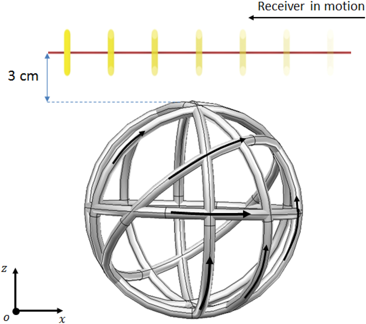Thus $p_{mu} = p_{mu \; max} \cdot 10{\rm \%} $ and crossover probability is set to p _cross  = 0.7. Table 1 shows the different dimensions, path lengths and heights for which system design has been achieved. (Here the term height refers to the z-coordinate of the receiver's path if we assume that this path is parallel to the x-coordinate axis as shown in Fig. 5.)

Fig. 5.

Transmitter topology.

Table 1.

Design conditions

Optimization results presented in this section correspond to systems designed to provide a magnetic field with a magnitude of 2 A/m along the receiver's path. Here, a receiver with a radius of 4 mm similar to those found in micro-robots applications is considered. Table 2 shows the parameters of the designed systems when a path of 8 cm is considered. For this purpose, only systems using sets of six sources are presented (parameters listed in the table are shown in Fig. 4):

Table 2.

The transmitter's parameters

The topology of the multi-source transmitter corresponding to the first line of Table 2 is shown in Fig. 4:

Table 3 shows the parameters of the designed systems when a path of 12 cm is considered (parameters listed in the table are shown in Fig. 4).

Table 3.

The transmitter's parameters

C) Model's frequency limit

The validity of the model proposed here depends on both frequency and distance. These two parameters are involved in the expression of the magnetic potential vector:

(16) $$\vec A = \displaystyle{{\mu _0} \over {4\pi}} \int \limits_l \displaystyle{{\vec i(r)} \over R}e^{ - jkR} dl,$$

where k = (2π/λ) is the wave number and λis the wavelength.

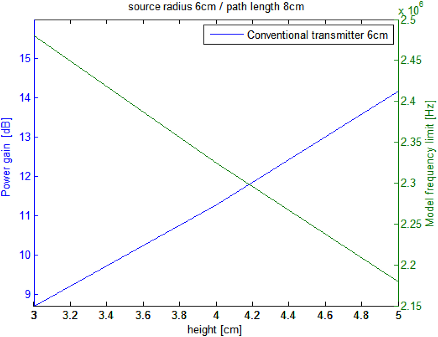
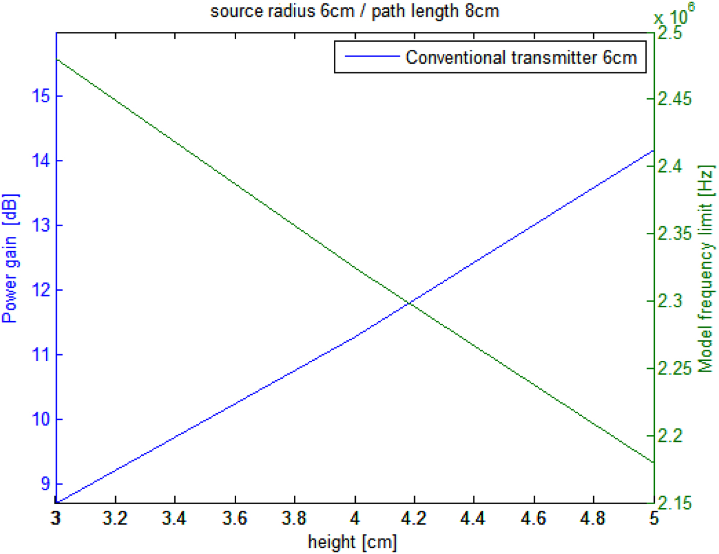
The frequency which is present in the exponential term e ^−jkR makes the calculation of the integral above impossible for a magnetic dipole. However, the evolution of this term shows that for a given maximum source-to-receiver distance real(e ^−jkR ) ≈ 1 as long as the operation frequency is lower than the frequency limit. While for higher frequencies, the real part starts decreasing and introduces an error in the magnetic field estimation. Consequently, the model's frequency limit will be represented by the green line in Figs 8–11 of which the values have been obtained according to the kR coefficient expression:

(17) $$\eqalignno{kR &= \displaystyle{{2\pi} \over \lambda} \cdot \max \left( {\sqrt {(z + 2 \cdot r_s \cdot \sin (\theta ))^2 + \left( {r_s \cdot \cos (\theta ) + \displaystyle{{l_p} \over 2}} \right)^2}} \right) \cr& = 0.001,}$$

wherez is the receiver height, r _s is the source radius, and l _p is the path length.

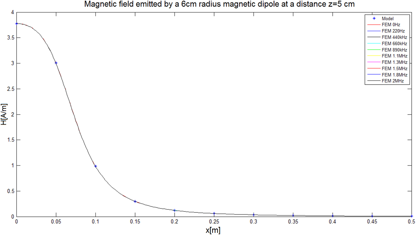
Thus, the frequency limit for a 6 cm radius transmitter placed at 5 cm from the receiver's path is equal to 2.15 MHz. Model validation of this configuration has been achieved using the FEA tool COMSOL for a transmitter of a 6 cm radius and 1 A current. The emitted magnetic field norm has been compared at a distance of z  =  5 cm and a path length of 50 cm along the x-axis (Fig. 6):

Fig. 6.

Magnetic field norm emitted at a distance of z  =  5 cm along a 50 cm path length using both model and finite elements simulation for a frequency range going from 0 Hz to 2 MHz.

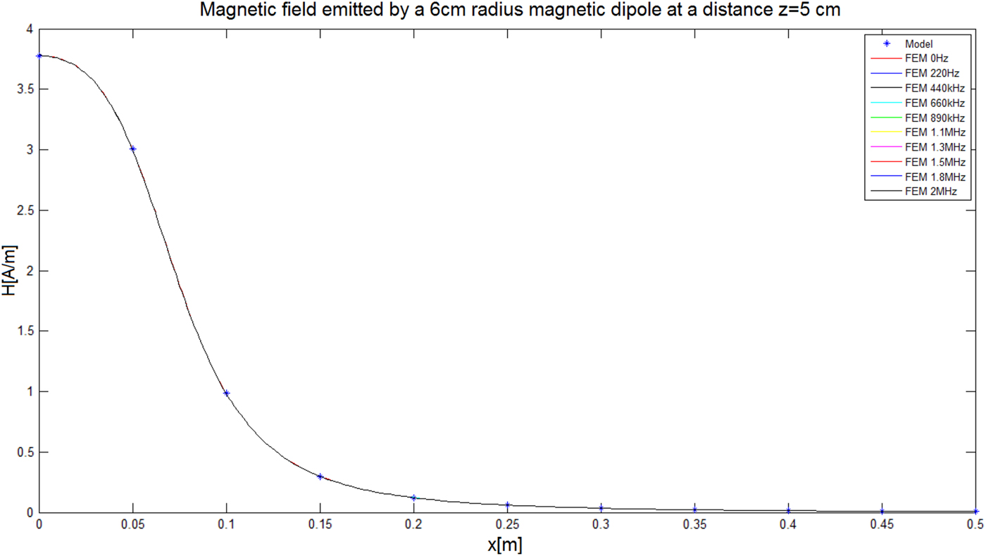
This comparison shows clearly that the suggested model in Section II is usable and results presented in the following section can be considered as reliable.

IV. DESIGN RESULTS

Receiver's dimensions in medical applications are usually small compared with the transmitter's size. Thus according to equation (1), the coupling factor (WPT efficiency) will drastically fall. This is why, in order to estimate the performance of the designed systems, the single-source-to-multi-source power gain has been estimated. Figure 8 shows this gain evolution when sources have a radius of 6 cm:

(18) $$G_{dB} = 10 \cdot log\left( {\displaystyle{{P_m} \over {P_s}}} \right) = 20 \cdot log\left( {\displaystyle{{V_m} \over {V_s}}} \right)$$

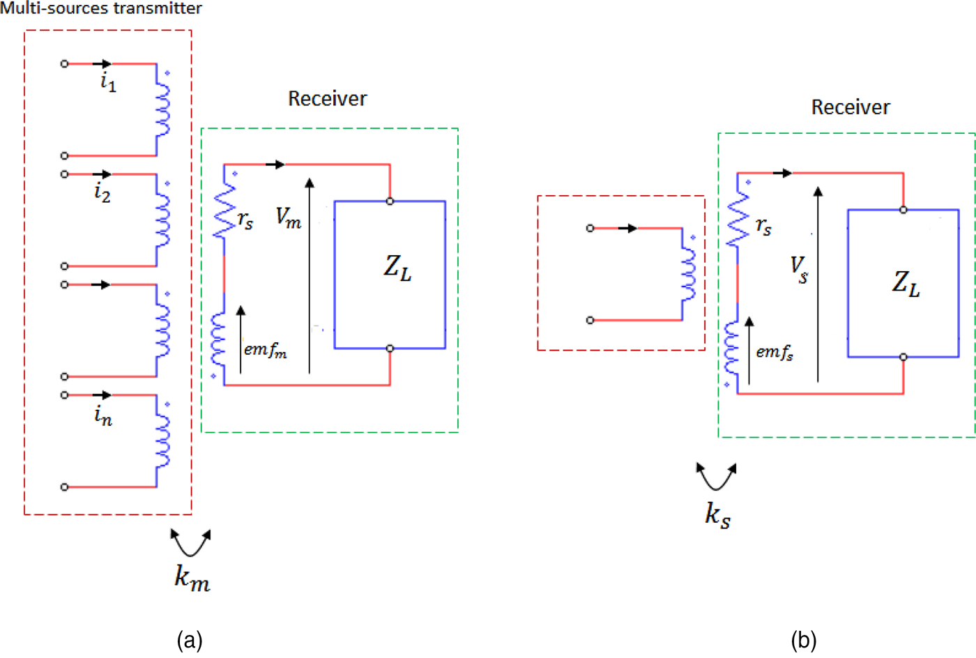
P _m and V _m are respectively the power and the voltage across the load when using a multi-source transmitter. While the same terms with the subscript “s” correspond to the single-source transmitter. The receiver's equivalent circuits in both configurations are presented in the figure below (Fig. 7):

Fig. 7.

(a) Schematic representation of the multi-source transmitter equivalent circuit, (b) schematic of conventional transmitter equivalent circuit.

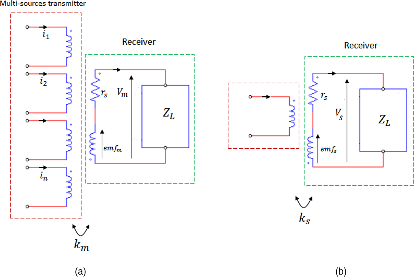
By neglecting the receiver's coil resistance r _r the voltage across the load becomes:V _m  = emf _m and V _s  = emf _s . By considering sinusoidal currents at the transmitter, the induced emf can be written:

(19) $$emf_m = - j\omega \cdot B_m \cdot cos(\theta _m ) \cdot A$$

and

$$\; emf_s = - j\omega \cdot B_s \cdot cos(\theta _s ) \cdot A.$$

By considering the receiver path parallel to (ox):

(20) $$emf_m = - j\omega \cdot B_{mx} \cdot A = V_m $$

and

(21) $$emf_s = - j\omega \cdot B_{sx} \cdot A = V_s. $$

For gain estimation, the power is calculated for transmitters with the same radius. However, the current injected within the single-source conventional transmitter is equal to the sum of the currents flowing in each source of the multi-source transmitter:

(22) $$G_{dB} = 20 \cdot log\left( {\displaystyle{{B_{mx}} \over {B_{sx}}}} \right).$$

Figure 8 shows the gain evolution obtained with transmitters containing six sources of 6 cm radius each along an 8 cm length path in terms of its height. It shows clearly how a set of sources improves the power transfer. For instance, we observe that the power gain is enhanced up to 14 dB at a height of 5 cm when a multi-source transmitter is used. The green line represents the frequency limit of the transmitter's model.

Fig. 8.

Power gain for a multi-source transmitter of 6 cm radius over a path of 8 cm.

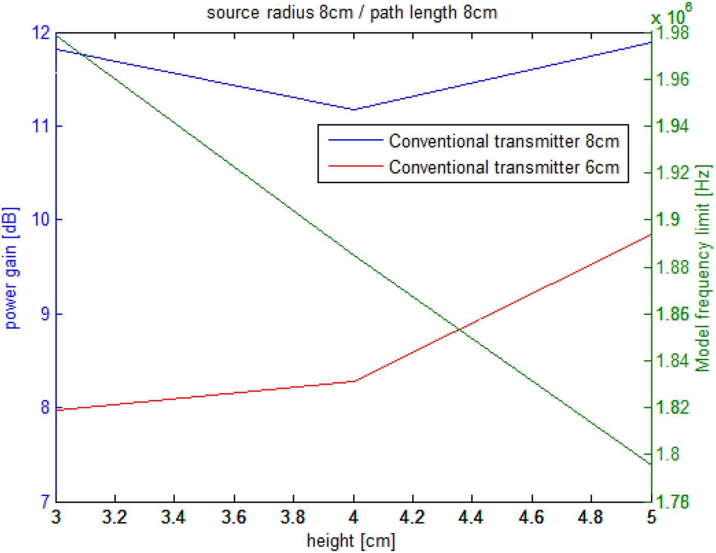
While Fig. 9 shows the evolution of the power gain as well as the frequency limit for transmitters containing six sources of 8 cm radius along an 8 cm length path in terms of its height. Even though the maximum gain has decreased, we notice that a bigger source provides a more or less constant gain over the considered heights. The curve in red represents the power gain when the new current sum is injected within a conventional transmitter of a 6 cm radius. This curve shows that power transfer gain reaches 10 dB.

Fig. 9.

Power gain for a multi-source transmitter of 8 cm radius over a path of 8 cm.

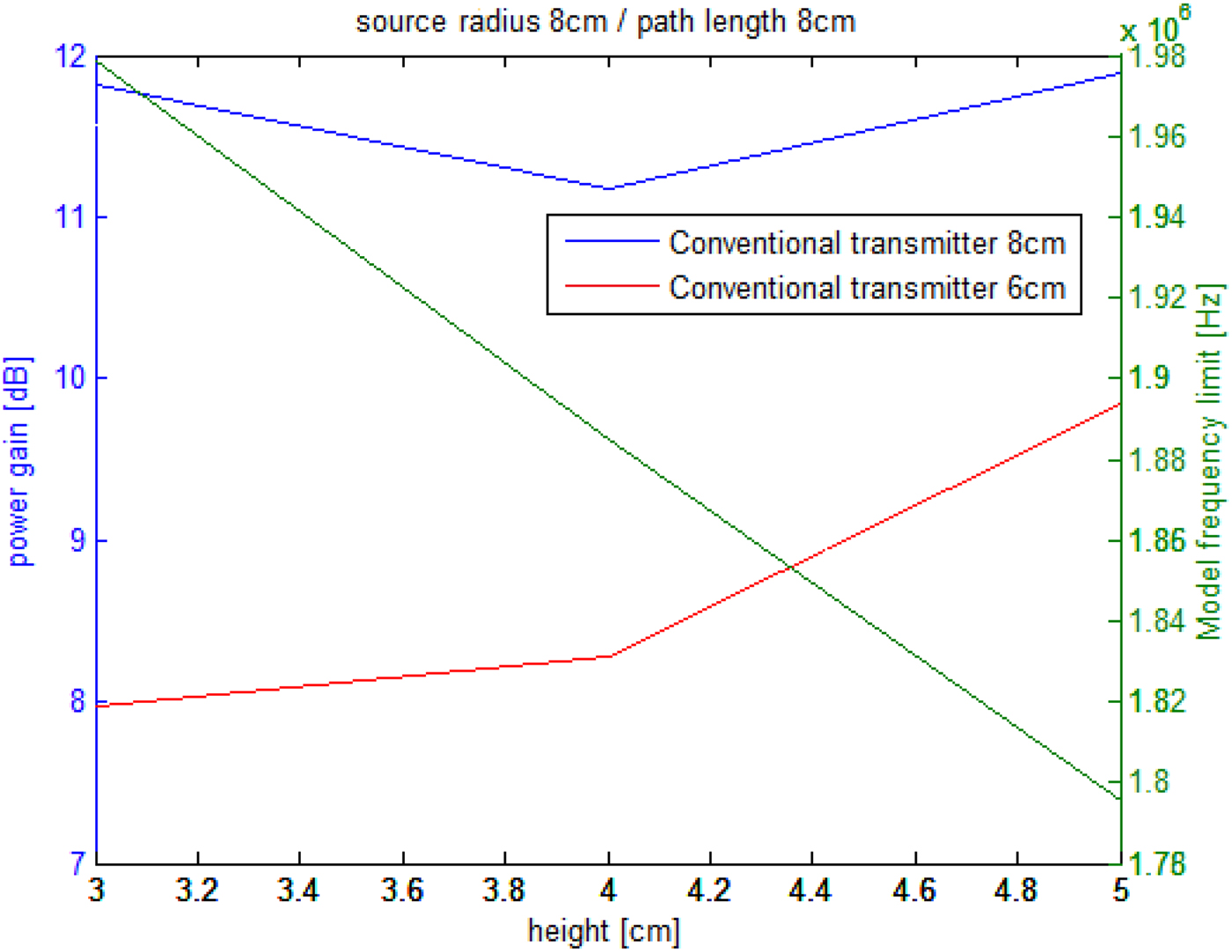
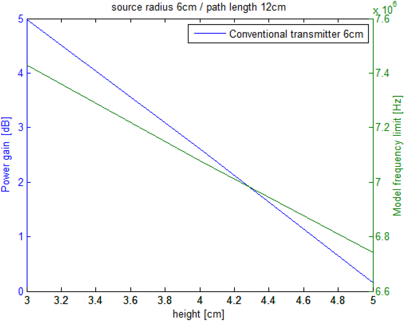
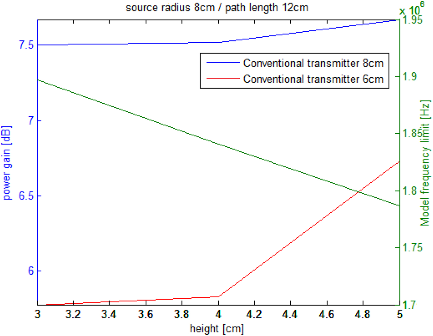
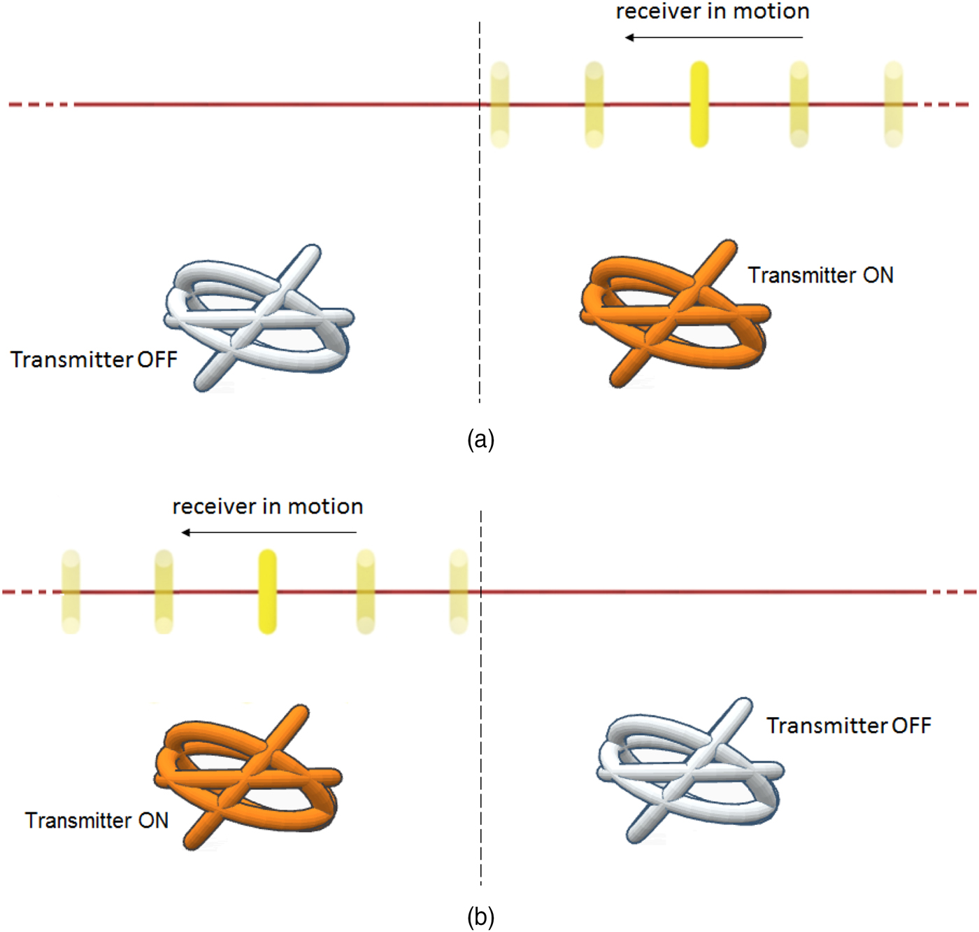
Figure 10 shows the gain evolution for a path length of 12 cm. it appears that using a transmitter containing sources of 6 cm radius does not provide a good enough gain. Indeed, when the receiver path is placed at 5 cm height, the gain is 0 which means that the multi-sources transmitter transfers the same power as a conventional single-source transmitter (Fig. 11). However, the transmitter containing sources with a radius of 8 cm provides an interesting power gain which enhances the power transfer up to 7.6 dB at 5 cm height. This result implies that for a longer path it is recommended to use a larger source. However, increasing the dimensions of the system every time the path gets longer may not be the best solution. This is why the association of different multi-source transmitters shown in Fig. 12 is suggested. Transmitters in such a configuration are activated alternatively depending on the receiver's position. This way, a transmitter is turned ON when the receiver is moving along its corresponding section. Thus, from the obtained results; an association of multi-source transmitters containing sources of 6 cm radius over an infinite length path; enhances the power transfer up to 5 dB (see Fig. 12).

Fig. 10.

Power gain for a multi-source transmitter of 6 cm radius over a path of 12 cm.

Fig. 11.

Power gain for a multi-source transmitter of 8 cm radius over a path of 12 cm.

Fig. 12.

Association with series of multi-source transmitters for an infinite length path.

V. LOSS DISCUSSION

Even though the work presented here treats about transmitter's design, it is worth it to mention that the transmitter in question does not affect the WPT system (converter  +  transmitter  +  receiver) overall efficiency. On the contrary, it helps to decrease it. If we consider resonant converters and where conduction losses represent a serious problem (switching losses being considerably reduced and considered negligible at high-power levels); this concept allows to considerably reduce them.

By considering that conduction losses depend on the current square, splitting the current through different sources will divide the total conduction losses by the number of sources (roughly) which makes the conduction losses much lower than in a conventional system.

This represents the other big advantage of the concept presented here and makes its implementation more interesting.