2. MODEL SELECTION CRITERIA FOR MOMENT CONDITION MODELS

Our notation closely follows Andrews and Lu (2001). Let g(X;γ) be the collection of moment conditions under consideration. Let b be the model selection vector that selects the elements of γ ∈ R^p to be estimated, i.e., a p-dimensional vector of 0 and 1's where 1 indicates that the corresponding parameter element is to be estimated. Similarly, let c be the r-dimensional moment selection vector that selects the moment conditions in g(·) ∈ R^r to be used in the estimation. Let γ_b ≡ b% * %γ denote the subvector of γ that is estimated and let g_c(·) ≡ c% * %g(·;γ) denote the subvector of g(·) that is used in estimation, where % * % denotes Hadamard (element-by-element) product.

In what follows, we refer to (b,c) as a pair of moment and model selection vectors. We use |c| (resp. |b|) to denote the total number of moments (resp. parameters) selected by the pair (b,c). Furthermore, τ_c denotes the |c|-dimensional vector of Lagrange multipliers corresponding to the g_c(·) moment conditions selected by c in the construction of the GEL function described subsequently. Finally, |c| − |b| is the number of overidentifying restrictions, and throughout we assume that the model is identified. This in particular requires the necessary condition that |c| − |b| ≥ 0.

We follow Andrews and Lu (2001) in defining the following sets. Let

denote the space of (b,c) vectors, which can be viewed as the “parameter space” in the moment and model selection procedure. Furthermore, define the set

where Eg_c(·;γ_b) denotes the population value of the empirical moment g_c(X;γ_b). In other words,

is the set of “feasible” vectors (b,c) that select only models and moments that equal zero asymptotically for some parameter vector. Finally,

In short,

is the set of “feasible” selection vectors (b,c) that maximize the quantity |c| − |b|, the number of overidentifying restrictions. Also let

denote the common values of |c| − |b| for all the elements of

.

In the rest of the paper we restrict attention to the case when

is a singleton. This implies that the GEL-MSC estimator

defined in the next section converges to a constant and allows for the usual asymptotic distribution for the postselection parameter estimates. When

is not a singleton, although the consistency result of Proposition 1 continues to hold,

may still be random in the limit and the asymptotic distribution for the postselection parameter estimates can be rather involved. Pötscher (1991) provides a detailed analysis of this important difference.

2.1. Generalized Empirical Likelihood-Based Model Selection Criteria

The GEL-MSC estimator,

, minimizes GEL-based MSC over

. The criterion function is defined as

where the GEL function (Newey and Smith, 2000) is defined as

Both h(·), a strictly increasing function, and the sequence κ_n are specified by the researcher. The carrier function ρ(v) is a function of a scalar v that is concave on its domain

, an open interval containing 0. It is normalized so that ρ(0) = 0, [dtri ]ρ(0) = −1, and [dtri ]²ρ(0) = −1, where [dtri ]ρ(·) and [dtri ]²ρ(·) correspond to the first and second derivatives of ρ(v), respectively. Therefore the GEL-MSC is the usual GEL criterion function, augmented by a penalty function that varies with the number of overidentifying restrictions and also with the number of observations.

The GEL function nests several special cases of interest: when ρ(v) = log(1 − v) the GEL function corresponds to the EL function; for ρ(v) = 1 − e^v it corresponds to the ET estimator; and a quadratic ρ(·) corresponds to the continuous updating estimator. Discussions of these estimators can be found in Newey and Smith (2000). Throughout the paper we assume that the data X_t are stationary and ergodic. The following assumptions on h(·) and κ_n are necessary for the consistency of the GEL-MSCs.

Assumption 1. h(·) is a strictly increasing function and κ_n → ∞ as n → ∞ and κ_n = o(n).

As in Andrews and Lu (2001), examples of GEL-MSCs that satisfy Assumption 1 include analogs of the Bayesian information criterion (BIC) and Hannan and Quinn information criterion (HQIC) based on GEL, both of which use h(x) = x:

2.2. Consistency of GEL Model Selection Criteria

A moment and model selection estimator

is defined to be consistent if

with probability converging to 1. In the following we give a set of assumptions under which the GEL-MSC estimator

provides a consistent moment and model selection estimator. These assumptions allow for both random sampling and dependent data.

Assumption 2. For each

,

(1) γ_b ∈ Γ_b, Γ_b is compact, τ_c ∈ Λ_c, and Λ_c is compact and contains a neighborhood of 0.

(2) There exist interior points γ* ∈ Γ_b and τ* ∈ Λ_c for each (b,c) such that

and

.

(3)

, where we denote

In particular, note that for

, we can take τ_c* = 0.

The interior point condition (2) requires that the moment condition model is not too misspecified and cannot be ruled out ex ante. For example, it can be violated if g(X_t;γ_b) > 0 with probability 1 for all γ_b ∈ Γ_b. The following lemma gives a set of sufficient conditions for Assumption 2.

LEMMA 1. Assumption (2) holds if condition (1) of Assumption 2 is satisfied and the following conditions are met for each (b,c):

A sufficient condition for the uniqueness of τ_c(γ_b) in condition (2′) of Lemma 1 is that the matrix Eg_c(X_t;γ_b)g_c(X_t;γ_b)′ is strictly positive definite for all (b,c) and γ_b ∈ Γ_b, because this implies that Eρ(τ_c′g(X_t;γ_b)) is strictly convex in τ_c for each γ_b. Sufficient conditions for condition (3′) of Lemma 1, which also imply condition (1′), are as follows: (i) g(X_t;γ_b) is uniformly continuous in γ_b; (ii) sup_{γb∈Γb,τc∈Λc}|ρ(τ_c′g(X_t;γ_b))| < ∞; (iii) X_t are independent and identically distributed (i.i.d.). Condition (ii) is satisfied if g(X_t;γ_b) is uniformly bounded.

Although beyond the results of this paper, much weaker conditions for uniform convergence using empirical process theory can be used to accommodate nonsmooth g_c(X_t;γ_b) (see, e.g., Andrews, 1994). Moreover, these weaker conditions can potentially allow for more general cases such as unbounded values of ρ(τ_c′g(X_t;γ_b)) for some realizations of X_t, which is important in the context of EL with unbounded moment functions. Consistency results under general conditions are developed by Newey and Smith (2000), who also exploit the concavity properties of the carrier function to bypass uniform convergence conditions and obtain

-consistency in one step.

Assumption 2 ensures that with probability converging to 1,

. This together with the next assumption will ensure also that

with probability converging to 1.

Assumption 3. For each

.

Sufficient conditions for Assumption 3 are developed in Kitamura and Stutzer (1997), Christoffersen, Hahn, and Inoue (2001), Chernozhukov and Hansen (2001), and Newey and Smith (2000), among others. Kitamura and Stutzer (1997) assume smooth moment functions. Chernozhukov and Hansen (2001) and Christoffersen et al. (2001) use empirical process theory (for nonsmooth quantile moment functions, see, e.g., Andrews, 1994). For completeness we collect some of these conditions used in the aforementioned papers in the following lemma.

LEMMA 2. Suppose that for each

, there exists a unique γ_b* ∈ Γ_b such that Eg_c(X_t;γ_b) = 0 if and only if γ_b = γ_b*. Assume that

and that the following conditions are satisfied:

Then Assumption 3 holds and

.

Note that although Lemmas 1 and 2 assume uniqueness of (γ_b*,τ_c*), this is not directly used in Assumptions 2 and 3. It is possible to relax these conditions to allow for nonunique γ_b*,τ_c*, i.e., models that are not point identified. These results are, however, beyond the scope of the paper. For correctly specified models, the results for

in Newey and Smith (2000) allow for unidentified moment conditions.

Given these conditions, the next proposition introduces the notion of consistency for GEL-based MSC.

Proposition 1. Under Assumptions 1–3, we have, with probability converging to 1,

for the pair

. In short, we say that the GEL-based MSC is consistent.

Other transformations of the GEL function can also be used to form MSCs. For example, because log(1 − x) = −x + o(x), the GEL-MSC may be redefined as

with corresponding conditions on κ_n. In particular, in the case of exponential tilting,

corresponds to the KLIC from the implied distribution to the true distribution in Kitamura and Stutzer (1997).

2.3. Time Series Data

The results of the previous section apply to both random sampling data and dependent data. For time series data, under suitable stationarity, ergodicity, and weak dependence conditions, condition (3) of Lemma (2) typically holds with (see, e.g., Andrews, 1991; Newey and West, 1987)

For i.i.d. data, S = Ω_c(γ_b*) and the GEL estimator

is as efficient as the optimally weighted GMM estimator for

. For time series data, although the GEL-MSC in the previous section is still consistent by Proposition 1, the estimator

is typically less efficient than the optimally weighted GMM.

To achieve efficiency with dependent data, the blocking methods of Kitamura and Stutzer (1997) (in the special case of ET) and Smith (1997) can be used to smooth the observations in constructing the GEL function. These authors define the blockwise GEL objective function as

and the blocks are constructed so that

. In what follows, we briefly discuss the modifications needed when Q_n(γ_b,τ_c) is used in place of Q_n(γ_b,τ_c) in constructing consistent GEL-MSCs. We only outline the results based on Kitamura and Stutzer (1997) and Smith (1997) and refer the reader to these papers for the complete set of stationary and weak dependence conditions and other regularity conditions that validate the blockwise GEL approach.

When

. On the other hand, for misspecified models in which

. Furthermore, when

Following the logic of Proposition 1, consistent MSC can be defined as before by minimizing

over (b,c), where the condition on κ_n is now modified to κ_n /K → ∞ and κ_n /n → 0.

2.4. Testing Procedure

Given the general consistency result of GEL-based MSC, we also describe the GEL analogs of two algorithms proposed in Andrews (1999) and Andrews and Lu (2001) to choose (b,c) consistently. In the following discussion we will focus on Q_n(γ_b,τ_c) rather than Q_n(γ_b,τ_c).

2.4.1. Downward testing procedure.

Andrews and Lu (2001) define the downward-testing model selection procedure as follows. Starting with vectors

for which |c| − |b| (the number of overidentifying restrictions) is the largest, perform tests (described in detail subsequently) with progressively smaller |c| − |b| (therefore the name “downward” testing) until a test is found that cannot reject the null hypothesis that the moment conditions considered are all correct for the given model. (Note that for each value of |c| − |b|, tests are carried out for each (b,c) in

with this value of |c| − |b|.) Let

denote the number of overidentifying restrictions (i.e., |c| − |b|) for this first test found to not reject the null. Given

, the downward testing estimator

is the vector that maximizes GEL_n(b,c) over

with

.

More formally, consider the GEL statistic:

. Under Assumptions 2 and 3, if the moment conditions are correctly specified (in the sense that τ_c* = 0 for the limit GEL problem min_γb max_τc[Eρ(τ_c′g(X_t;γ_b))]), then GEL_n(b,c) = O_p(1).

²

For random sampling data typically GEL_n(b,c), as defined in (1), converges in distribution to χ_|c|−|b|² under correct specification, although for consistent model selection we only need GEL_n(b,c) = O_p(1).

The downward-testing procedure looks for the first acceptance among

of the test whose rejection region is defined by

where χ_k²(α_n) denotes the (1 − α_n)th quantile of the chi-squared distribution with k = |c| − |b| degrees of freedom. The following consistency result can be shown for the downward-testing estimators

, which is analogous to Theorem 2 in Andrews and Lu (2001).

Proposition 2. If the sequence of critical values satisfies for each k

then under Assumptions 2 and 3,

.

2.4.2. Upward testing procedure.

The GELs can also be applied to the upward-testing procedure described in Andrews (1999). Starting with vectors

that have the smallest number of overidentifying restrictions |c| − |b|, we perform tests (analogous to those described for the downward-testing procedure previously) with progressively more overidentifying restrictions (i.e., larger |c| − |b|; therefore the name “upward testing”) until we find that all tests with the same value of |c| − |b| reject the null hypothesis that the moment conditions considered are all correct. Let

denote the largest value such that for all

, there is at least one

with |c| − |b| = k for which the null hypothesis is not rejected. Given

, we take the upward testing estimator

to be the vector that minimizes GEL_n(b,c) over

.

It is necessarily true that the upward testing procedure described here will never select a pair (b,c) with more overidentifying restrictions than the downward testing procedure; i.e.

To avoid selecting a pair (b,c) with too few overidentification conditions, an additional assumption (as in Andrews, 1999) is made to ensure consistency of

.

Assumption 4. For each

such that

, there exists (b,c) with |c| − |b| = k for which

.

Without this condition, the inequality (2) may hold strictly, even asymptotically. Note that this additional condition can be ensured by proper choice of the parameter space

for the selection vector (b,c). Under this additional condition, we state the following proposition.

Proposition 3. With probability converging to 1,

.

2.5. Analogy with Parametric Likelihood Model Selection Procedure

Andrews (1999) shows that the J-statistic-based MSC is analogous to standard MSC (such as the BIC, Akaike information criterion [AIC], and HQIC) often employed in parametric model selection procedures. When we use GEL to formulate the MSC, this analogy is very transparent because, in this case, an explicit likelihood- (or information-) based rationale also underlies the moment selection procedure, just as in the fully parametric case.

Andrews (1999) notes that his J-statistic MSC is analogous to the parametric MSC in the sense that, among correct models, this criterion would choose the more tightly specified model. Equation (6.6) in Andrews (1999) shows an equivalence result between the problem of maximizing the number of moment conditions (i.e., minimizing the number of excluded moment conditions) and minimizing the number of parameters, among correctly specified models. In this section, we show an analogous equivalence for GEL-based MSCs.

Under correct specification GEL is asymptotically equivalent to GMM estimation using the optimal weighting matrix. The use of GEL-based MSC also provides a transparent proof of this equivalence result by avoiding the issues associated with choosing the optimal weighting matrix in GMM estimation, which arise when considering the J-statistic.

Following Andrews (1999), we simplify notation by assuming that all the models under consideration are correctly specified, and we focus on the moment selection problem (involving the moment selection vector c and the associated Lagrange multipliers τ_c). Therefore, in the discussion that follows, we let

, the vector whose elements are all 1, and γ_b = γ throughout, and we assume that g_c(·) is sufficient for identification of γ. Our goal is to show the equivalence between

where g_c(·) is the subvector of g(·) selected by c, and

where g_−c(·) is the subvector of the totality of moment conditions g(·) that are excluded by the selection vector c. Here μ is of dimension r − |c|, where r is the total number of moment conditions under consideration. This equivalence is analogous to equation (6.6) in Andrews (1999) and implies that the moment selection problem can alternatively be viewed as a model (i.e., parameter) selection problem, with the augmented parameter vector (γ,μ)′.

The equivalence of (3) and (4) is easy to demonstrate; indeed, let

solve (3), i.e., satisfy the first-order conditions

Then it follows that

and

solves the problem in (4). Indeed, one can easily verify that the first-order conditions for problem (4), which can be written as

are necessarily satisfied at these parameter values. It is also immediately obvious that at these parameter values the two GEL functions are identical:

which is analogous to equation (6) in Andrews (1999). Thus the analogy between generalized empirical likelihood-based moment and model selection procedures and Andrews' J-statistic based procedures is complete. The use of GEL-based MSC allows us to generalize the likelihood-based rationale underlying the usual MSC for parametric models to semiparametric models in which the data-generating process is only partially specified via population moment restrictions.

3. MONTE CARLO EXPERIMENTS

In this section we report the results from a simple Monte Carlo study designed to compare MSC based on the J-statistic as proposed by Andrews (1999) and Andrews and Lu (2001) and also on two special cases of the GEL statistic: empirical likelihood and exponential tilting. Formally, these criteria are written as

using the same notation as in the previous sections.

Appropriate choices of the h(·) function and the sequence of constants, κ_n, deliver the BIC, AIC, and HQIC MSC. We also consider the choice of h(·) as the identity mapping and sequence of constants as

, which we refer to as root n information criterion (RNIC).

The model is specified by the set of equations

where u_t, η_t, and φ_t are all independently distributed N(0,1) random variables, truncated at −2 and 2. Both z_t and f_t are candidate instruments. By considering alternative values for the coefficient α the analysis can accommodate homoskedastic and heteroskedastic error structures. To this end, values of zero and a small positive constant are considered. The fact that E [f_tu_t] ≠ 0 implies that moment conditions constructed from the instrument f_t are invalid. Moment conditions are constructed from the following five possible instrument groups.

M1. constant, cos(z) + sin(z).

M2. constant, z, cos(z) + sin(z), cos(z).

M3. constant, cos(z) + sin(z), sin(f).

M4. constant, z, cos(z) + sin(z), cos(z), sin(f).

M5. constant, cos(z) + sin(z), cos(f), sin(f).

The econometrician is assumed to know that the M1 moment conditions are valid and seeks to determine the verity of the remaining moment conditions for estimation. In the preceding notation, M2 instruments are the true (b⁰,c⁰), M1 instruments are other consistent (b,c), and the remaining instrument groups contain inconsistent (b,c). Therefore, this model that we use for the Monte Carlo experiments satisfies the condition that

is a singleton. This is a case in which the limiting distribution of the postselection (for consistent MSCs) estimator is known to be the same as if (b⁰,c⁰) are picked a priori (see, e.g., Pötscher, 1991).

In the subsequent tables, these three groupings of instruments will be referenced by the abbreviations OC, Truth, and IC, respectively. The sin(·) and cos(·) functions are utilized as a convenient way to generate instruments. Following the suggestions in Andrews and Lu (2001), we have chosen the moment conditions in these models so that (i) there is a noticeable difference in efficiency between the estimators that use all the correct moment conditions and the estimators that use only those moment conditions that are known to be correct and (ii) there are noticeable biases in the estimators that use incorrect moment conditions. This setup allows for gains to be exploited from a good moment selection procedure. It is clear that the exercise can be generalized to allow also for “model selection” over sets of possible regressors.

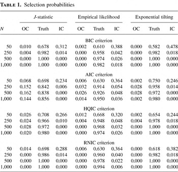
Following Andrews and Lu (2001), we assess the relative performance of these MSC by comparing the probability with which the three MSCs select the true (b⁰,c⁰); other consistent (b,c); and inconsistent (b,c). MSC that have both a high probability of selecting the true model and a low probability of selecting inconsistent models are preferred. The performance of postselection estimators is assessed by comparison of the bias and root mean squared errors (RMSEs) of the estimated slope coefficient of each model. The rejection rates for a 5% t-test that each of these parameter estimates is equal to the true value of unity are also computed. These statistics are reported for estimation based on each of the five instrument sets and for each of the four MSC, to give a total of nine postselection model results. Because there are three estimation methods—GMM, EL, and ET—we report postselection results for a total of 27 models. Results based on the proposed EL- and ET-based MSC relative to the GMM-based approach are of most interest. The results based on each of the five possible instrument groups are presented for comparison, with the infeasible estimator resulting from the use of M2 giving the “ideal” benchmark. The results are based on 500 repetitions for four sample sizes, N = 50, 250, 500, and 1,000.

Table 1 details the probabilities of selecting the true, other consistent, and inconsistent models under assumption of a homoskedastic error structure (α = 0). For each estimation method, results are collected by each of the four proposed penalty functions (BIC, AIC, HQIC, and RNIC). Considering the BIC and

criteria, it is clear that the J-MSC outperforms both the MSCEL and MSCET for the smaller sample sizes. The probability of selecting the true model is higher by 5% and the probability of selecting a misspecified model lower by up to 10%. As the sample size increases the discrepancy between the J-MSC and MSCET vanishes, whereas the MSCEL has slightly higher probability of selecting an inconsistent model. Under the AIC criterion, the MSCET outperforms both J-MSC and MSCEL at all sample sizes. The gains are of the order of 10%, though they are somewhat smaller when compared to MSCEL at larger sample sizes. The inconsistency of the AIC selection procedure is immediate from the J-MSC results (though interestingly, in the context of this model, the inconsistency of the AIC criterion seems to be small under EL- and ET-based methods and AIC appears able to distinguish the correct model with high probability). Finally, for HQIC, J-MSC again performs better in the smallest sample size, whereas MSCET is marginally better as N increases. For all models, we note that the MSC appear to perform reasonably well for sample sizes above 250.

Selection probabilities

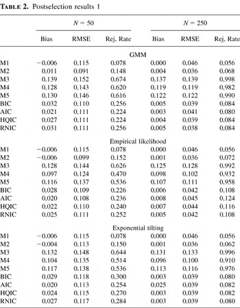
Table 2 presents the bias, RMSEs, and rejection rates of the postselection estimates of the model's slope coefficient for the two smallest sample sizes. To clarify notation, for each estimation method (GMM, EL, and ET), the results based on each of the five instrument groups are labeled M1–M5, whereas those postselection results arising from the four MSC are labeled by the corresponding penalty term: i.e., BIC, AIC, HQIC, and RNIC.

Postselection results 1

Considering the results obtained under GMM, it is immediate that misspecification can lead to poor postselection results. If estimates are based on any of the incorrectly specified models (M3–M5) then the bias is some 10 times greater than the infeasible estimator (M2), with a corresponding deterioration in the RMSEs. For such models, the rejection rate in small sample size (N = 50) for a 5% t-test that the slope coefficient is equal to the true value of unity is likely to be rejected over 60% of the time. Thus, misspecification can clearly lead to erroneous conclusions. In contrast, for the MSC, we note that the performance of the postselection estimators is much closer to the infeasible estimator. The bias is approximately three times that under M2, whereas the RMSEs are marginally higher. Correspondingly, the rejection rates of a 5% t-test are reduced for each of the MSC relative to misspecified models to about 20%. Of the four selection criteria, the AIC seems to perform best in small sample sizes (N = 50), even though it is theoretically inconsistent. This does not appear too surprising, given the finite-sample bias and size distortion when N = 50 and the fact that the selection probabilities for AIC compare very favorably to other MSCs in this small sample size of N = 50. In addition, the post-AIC estimators are still consistent, and the distortion in the sampling distribution might not be significant for the model we consider and for small sample sizes. For larger sample sizes, however, AIC clearly does not perform quite as well as other consistent MSCs, even though the discrepancy appears marginal. As the sample size increases to 250, the differences between results based on the true model and those based on each of the four selection criteria are remarkably small. The biases are comparable, whereas the RMSEs and rejection rates are slightly higher.

For the EL- and ET-based results, the same broad patterns of results are observed. However, comparison of these results to those obtained under GMM suggests that the former have smaller bias and comparable RMSEs for the smallest sample size, though a slightly higher rejection rate under ET. For the N = 250 sample, ET seems to perform better than EL. The bias is half as much and the RMSEs somewhat smaller. Relative to GMM, ET seems to perform marginally better.

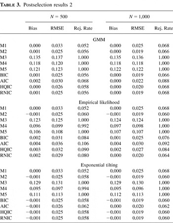
Finally, Table 3 presents an identical set of results to those in Table 2 but for the sample sizes N = 500 and 1,000. Consistent with the results of Table 1, as N increases from 250 to 1,000 the bias is essentially eliminated for GMM- and ET-based models and the RMSEs fall at a rate consistent with the increase in sample size. For both larger sample sizes the ET-based results are marginally better than the GMM-based results, whereas the EL-based results are somewhat worse. For ET and GMM the BIC, HQIC, and RNIC MSC nearly always select the true model for the largest sample size. As expected, for large N the rejection rates go to 1 for misspecified models and are in the neighborhood of 5% for the infeasible model and all MSC-based selection models.

Postselection results 2

We also study the performance of selection probabilities and postselection estimators in a heteroskedastic version of the preceding model. The Monte Carlo results for a heteroskedastic case are not reported given their similarity to the homoskedastic results, but they can be obtained at the Web address www.princeton.edu/^∼doubleh.