II. SYSTEM MODELING AND OUTPUT POWER ANALYSIS

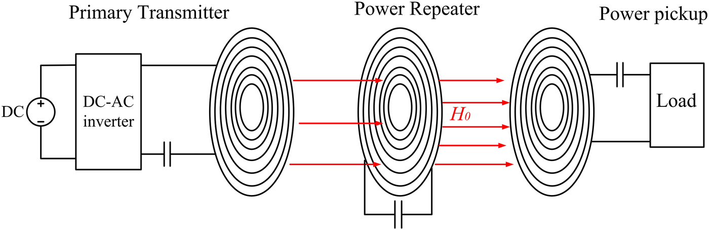
Figure 1 shows a layout of an IPT system with a primary transmitter, a passive power repeater, and a power pickup. The power repeater is placed between the primary coil and the power pickup coil for relaying the magnetic field generated by the primary coil to the pickup coil. The primary transmitter contains a DC power supply, a DC–AC inverter, and a primary coil which is series tuned with a capacitor to the nominal frequency. The power repeater is formed by a lumped coil tuned using a capacitor to the frequency of interest. A pickup coil, a load resistor, and a tuning capacitor are in series connected to form the power pickup, and the pickup coil is tuned to the nominal frequency.

Fig. 1.

An overview of a typical layout of an IPT system with a passive power repeater.

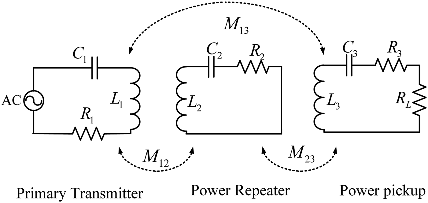
The equivalent steady-state circuit model of the IPT system is shown in Fig. 2. The DC power supply and DC–AC inverter is modeled as a constant voltage source. The transmitting coil is modeled as an inductor L ₁ with an Equivalent Series Resistance (ESR) R ₁, and a capacitor C ₁ is added to tune the transmitting coil. The coil of the power repeater is modeled as an inductor L ₂ with an ESR R ₂, and it is tuned with a capacitor C ₂. The power pickup coil is modeled as an inductor L ₃ with an ESR of R ₃, and it is in series connected with a tuning capacitor C ₃ and load resistor R _L. Inductors L ₁ and L ₂ are magnetically linked by mutual inductance M ₁₂. The mutual inductance M ₂₃ magnetically links inductors L ₂ and L ₃, and the mutual inductance M ₁₃ magnetically links inductors L ₁ and L ₃.

Fig. 2.

The equivalent system steady-state circuit model.

The Kirchhoff's voltage law (KVL) is applied to each resonant circuit of the system:

(1)$$\eqalign{& j\omega M_{12}I_2 + j\omega M_{13}I_3 + (X_1j + R_1)I_1 = V_s \cr & j\omega M_{12}I_1 + j\omega M_{23}I_3 + (X_2j + R_2)I_2 = 0 \cr & j\omega M_{13}I_1 + j\omega M_{23}I_2 + (X_3j + R_3 + R_L)I_3 = 0.} $$

where I ₁, I ₂, and I ₃ are the currents going through the primary coil, the coil of power repeater, and the load resistance, respectively, V _s is the input voltage, X ₁, X ₂, and X ₃ are the reactances of the resonant circuit of primary transmitter, the power repeater, and the power pickup, respectively, and they are represented as

(2)$$\eqalign{& X_1 = \omega L_1 - \displaystyle{1 \over {\omega C_1}},\quad X_2 = \omega L_2 - \displaystyle{1 \over {\omega C_2}}, \cr & X_3 = \omega L_3 - \displaystyle{1 \over {\omega C_3}}.}$$

As both the primary coil and the pickup coil are tuned to the nominal frequency, X ₁ and X ₃ equal to zero. So (2) can be simplified as (3):

(3)$$\eqalign{& j\omega M_{12}I_2 + j\omega M_{13}I_3 + R_1I_1 = V_s \cr & j\omega M_{12}I_1 + j\omega M_{23}I_3 + (X_2j + R_2)I_2 = 0 \cr & j\omega M_{13}I_1 + j\omega M_{23}I_2 + (R_3 + R_L)I_3 = 0.} $$

By simultaneously solving three equations in (3), the output current is achieved as (4):

(4)$$I_3 = - \displaystyle{{M_{12}M_{23}V_s\omega ^2 + j\omega M_{13}V_s(R_2 + X_2j)} \over \matrix{M_{12}^2 \omega ^2(R_3 + R_L) - 2jM_{12}M_{13}M_{23}\omega ^3 + (R_2 + X_2j)M_{13}^2 \omega ^2 \hfill \cr + R_1M_{23}^2 \omega ^2 + R_1(R_3 + R_L)(R_2 + X_2j) \hfill} }.$$

By substituting the amplitude of I ₃ into (5), the output power is obtained as (6):

(5)$$P_o = \left \vert {I_3} \right \vert ^2R_L,$$

(6)$$P_o = \displaystyle{{V_s^2 \omega ^2({(M_{13}X_2 - M_{12}M_{23}\omega )}^2 + M_{13}^2 R_2^2 )R_L} \over \matrix{\left( { - 2M_{12}M_{13}M_{23}\omega ^3 + X_2M_{13}^2 \omega ^2 + R_1X_{{2}}(R_3 + R_L)} \right)^2 \hfill \cr \eqalign{&+ \big( M_{12}^2 (R_3 + R_L)\omega ^2 + M_{13}^2 R_2\omega ^2 + M_{23}^2 R_1\omega ^2 \cr &+ R_1R_2(R_3 + R_L) \big)^2} \hfill} }.$$

Equation (6) shows the relationship between the output power and the reactance X ₂ of the power repeater. For given mutual inductances between the coupled coils, ESRs of coupled coils, load resistance, and a system operating frequency, the relationship between the output power of an IPT system and the reactance of power repeater can be achieved by using optimization tools such as MATLAB.

III. EFFECT OF POWER REPEATER TUNING ON OUTPUT POWER

A) Determining the critical tuning capacitance between enhancing and reducing the output power

The output power of the IPT system without the passive power repeater is set to be the reference for determining whether the output power is enhanced and reduced by the power repeater. For the IPT system without the passive power repeater, the system equation (7) can be derived by applying KVL to the primary and pickup resonant circuits:

(7)$$\eqalign{& j\omega M_{13}I_{3 - noR} + R_1I_{1 - noR} = V_s \cr & j\omega M_{13}I_{1 - noR} + R_3I_{3 - noR} = 0.} $$

where I _1−noR and I _3−noR are the current going through the primary coil and the load resistance of the IPT system when there is no passive power repeater.

By simultaneously solving two equations in (7), I _3−noR is obtained. Multiplying the square of the amplitude of I _3−noR by the load resistance R _L, the output power of the IPT system without the power repeater is obtained as

(8)$$P_{o - noR} = \displaystyle{{(M_{13}^2 R_LVs^2\omega ^2)} \over {{(\omega ^2M_{13}^2 + R_1R_3 + R_1R_L)}^2}}.$$

The power ratio between P _o and P _o−noR is represented as

(9)$$r = \displaystyle{{P_o} \over {P_{o - noR}}}.$$

The output power is enhanced by the power repeater when the ratio is larger than 1, and the output power is reduced when the ratio is smaller than 1. By substituting (6) and (8) into (9) and solving (9) when it equals to 1, the critical reactance X _2−cr which sets up the boundary between increasing or decreasing of the system output power is obtained as (10). By substituting (10) into (2), the corresponding tuning capacitance is obtained as (11):

(10)$$X_{2 - Cr} = \displaystyle{\matrix{M_{12}^2 M_{23}^2 \omega ^2 + M_{13}^2 R_2^2 \hfill \cr - \left( \matrix{M_{13}^2 \left( \matrix{\left( \matrix{M_{12}^2 \omega ^2(R_3 + R_L) + M_{13}^2 R_2\omega ^2 \hfill \cr + M_{23}^2 R_1\omega ^2 + R_1R_2(R_3 + R_L) \hfill} \right)^2 \hfill \cr + 4M_{12}^2 M_{13}^2 M_{23}^2 \omega ^6 \hfill} \right) \hfill \cr /\left( {M_{13}^2 \omega ^2 + R_1(R_3 + R_L)} \right)^2 \hfill} \right) \hfill} \over \matrix{2M_{12}M_{13}M_{23}\omega \hfill \cr - \left( {4M_{12}M_{13}^3 M_{23}\omega ^3/M_{13}^2 \omega ^2 + R_1(R_3 + R_L)} \right) \hfill} },$$

(11)$$C_{2 - Cr} = \displaystyle{1 \over {\omega ^2L_2 - \left( {\displaystyle{\matrix{M_{12}^2 M_{23}^2 \omega ^2 + M_{13}^2 R_2^2 \hfill \cr - \left( \matrix{M_{13}^2 \left( \matrix{\left( \matrix{M_{12}^2 \omega ^2(R_3 + R_L) + M_{13}^2 R_2\omega ^2 \hfill \cr + M_{23}^2 R_1\omega ^2 + R_1R_2(R_3 + R_L) \hfill} \right)^2 \hfill \cr + 4M_{12}^2 M_{13}^2 M_{23}^2 \omega ^6 \hfill} \right) \hfill \cr /\left( {M_{13}^2 \omega ^2 + R_1(R_3 + R_L)} \right)^2 \hfill} \right) \hfill} \over \matrix{2M_{12}M_{13}M_{23} \hfill \cr - \eqalign{&\big(4M_{12}M_{13}^3 M_{23}\omega ^2/M_{13}^2 \omega ^2 \cr &+ R_1(R_3 + R_L)\big)} \hfill} }} \right)}},$$

$$\eqalign{A & = \left( {M_{12}^2 R_2(R_3 + R_L) + M_{23}^2 R_1R_{2{\rm \;}}} \right)M_{13}^4 \cr & \quad+ {\rm \;} \left( {\displaystyle{{M_{12}^4 {(R_3 + R_L)}^2} \over 2} + \displaystyle{{M_{23}^4 R_1^2} \over 2}} \right)M_{13}^2,}$$

$$\eqalign{B & = - M_{12}^2 M_{23}^2 R_1^2 (R_3 + R_L)^2 - M_{13}^2 (M_{12}^2 R_1R_2(R_3 + R_L)^2 \cr & \quad + M_{23}^2 R_1^2 R_2 (R_3 + R_L)),}$$

$$\eqalign{C & = (M_{12}^2 M_{13}^2 \omega ^2 + M_{23}^2 R_1^2 )(M_{12}^2 (R_3 + R_L)^2 + \omega ^2M_{13}^2 M_{23}^2 ) \cr & \quad \times \left( \matrix{(M_{12}^4 M_{13}^2 \omega ^4 + 4\omega ^2M_{12}^2 M_{13}^2 R_2R_1 + {\rm \; }\omega ^2M_{12}^2 M_{23}^2 R_1^2 \hfill \cr + {\rm \; }4M_{13}^2 R_1^2 R_2^2 )(R_3 + R_L)^2 + (8\omega ^2M_{13}^4 R_1R_2^2 + {\rm \; }4\omega ^2M_{13}^2 M_{23}^2 R_1^2 R_2 \hfill \cr + 4\omega ^4M_{12}^2 M_{13}^4 R_2)(R_3 + R_L) + {\rm \; }M_{13}^2 \omega ^4(2M_{13}^2 R_2 + M_{23}^2 {\rm R}_1)^2 \hfill \cr + M_{12}^2 M_{13}^4 M_{23}^2 \omega ^6) \hfill} \right),} $$

$$D = M_{12}M_{13}M_{23}( - M_{13}^4 \omega ^4 + R_1^2 (R_3 + {\rm \;} R_L)^2).$$

Equation (11) shows the critical tuning capacitance which sets up the boundary between increasing and decreasing the output power. By setting (9) to larger than 1 and solving the equation, it is found that the output power is enhanced when the tuning capacitance of a passive power repeater is smaller than the critical capacitance. The output power is found to be reduced when the tuning capacitance of a passive power repeater is larger than the critical tuning capacitance by solving (9) when it is set to be smaller than 1. The finding of the critical tuning capacitance can help to choose the right range of tuning capacitances of passive power repeaters for increasing the output power of the IPT systems.

B) Determining the optimal tuning capacitances

Equations (6) and (8) are substituted into (9), and then the first differentiation of (9) is set as

(12)$$\displaystyle{{dr} \over {dX_2}} = 0.$$

By solving (12), the optimal reactances X _2−op1 and X _2−op2 of a passive power repeater are obtained as (13):

(13)$$\eqalign{& X_{2 - op1} = \displaystyle{{3\omega M_{12}M_{23}} \over {2M_{13}}} - \displaystyle{{(2\omega ^3A - 2\omega B + \sqrt C )} \over {2D}} \cr & X_{2 - op2} = \displaystyle{{3\omega M_{12}M_{23}} \over {2M_{13}}} + \displaystyle{{(2\omega B - 2\omega ^3A + \sqrt C ),} \over {2D}}} $$

where the representations of A, B, C, and D are presented above.

To check whether the two optimal capacitances are for achieving the maximum output power, equation (9) is differentiated with respect of X ₂ again. By substituting X _2−op1 and X _2−op2 into the second differentiation, respectively, it is found that neither of the second differentiations equal to zero, which indicates X _2−op1 and X _2−op2 are not inflection points. Therefore, one of them is for achieving maximum output power, and the other one is for obtaining minimum output power.

To determine the optimal tuning capacitance for achieving the maximum output power, the output powers P _op1 and P _op2 are obtained by substituting X _2−op1 and X _2−op2 into (6), respectively. By subtracting P _op1 by P _op2, (14) is obtained:

(14)$$\eqalign{& P_{op1} - P_{op2} \cr & \quad \quad = \displaystyle{{R_LV_{\rm s}^2 \omega ^3\sqrt C } \over {{\left[ \matrix{((\omega ^2M_{13}^2 + R_1 (R_3 + R_L{\rm )})(\omega ^2M_{12}^2 (R_3 + R_L{\rm )}^2 \hfill \cr + \omega ^2M_{13}^2 R_2 + \omega ^2M_{23}^2 R_1 + R_1R_2 (R_3 + R_L{\rm )}) \hfill} \right]}^2}}.}$$

Equation (14) shows the difference between P _op1 and P _op2, and it is found to be positive, which indicates X _2−op1 is the reactance for achieving maximum output power, and X _2−op2 is the reactance for obtaining minimum output power. By substituting X _2−op1 and X _2−op2 into (2), the corresponding tuning capacitances are obtained as in (15):

(15)$$\eqalign{& C_{2 - P\max } = \displaystyle{1 \over \matrix{\omega ^2L_2 - ((3\omega ^2M_{12}M_{23}/2M_{13}) \hfill \cr - ((2\omega ^3A - 2\omega B + \sqrt C ) \hfill \cr /2M_{12}M_{13}M_{23}( - M_{13}^4 \omega ^4 + R_1^2 (R_3 + {\rm \; }R_L)^2))) \hfill} }, \cr & C_{2 - P\min } = \displaystyle{1 \over \matrix{\omega ^2L_2 - ((3\omega ^2M_{12}M_{23}/2M_{13}) \hfill \cr + ((2\omega ^3A - 2\omega B + \sqrt C ) \hfill \cr /2M_{12}M_{13}M_{23}( - M_{13}^4 \omega ^4 + R_1^2 (R_3 + {\rm \; }R_L)^2))) \hfill} }.} $$

Equation (15) gives the optimal tuning capacitances corresponding to the maximum and minimum output powers. The maximum output power can be achieved when the tuning capacitance of power repeater equals C _2−Pmax, and the minimum output power can be obtained when the tuning capacitance is C _2−Pmin.

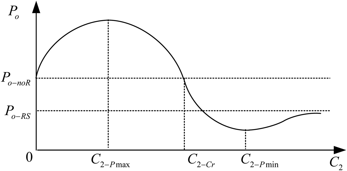
These two optimal tuning conditions are also related to power enhancing and reducing characteristics of the power repeater. Combining the finding of the range of tuning capacitance for increasing and reducing the output power, Fig. 3 is plotted to illustrate the general relationship between the output power and the tuning capacitance of a passive power repeater, and key tuning capacitances are labeled in the plot. Compared to the original IPT system without a passive power repeater, the output power P _o of the IPT system with a passive power repeater can be higher when the tuning capacitance of power repeater C ₂ is smaller than the critical tuning capacitance C _2−Cr; and lower when C ₂ is larger than C _2−Cr. The maximum and minimum output powers are obtained at C _2−Pmax and C _2−Pmin, respectively. P _o approaches P _{o−R S} as shown in Fig. 3 when the tuning capacitance increases to infinite, corresponding to the situation when the power repeater is short circuited. This research focuses on enhancing the output of the IPT system, so the tuning capacitance of the power repeater is smaller than the critical tuning capacitance C _2−Cr.

Fig. 3.

Illustrations of the general relationship between the output power and the tuning capacitance of the power repeater.

IV. EXPERIMENTAL VERIFICATION

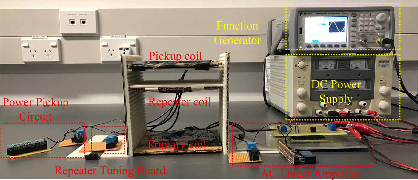
The experimental setup is shown in Fig. 4. This setup includes a DC power supply, a waveform function generator, an AC linear power amplifier, a frame for holding coupled coils, and a power pickup circuit. The function generator inputs an AC voltage signal with an amplitude of 500 mV and a frequency of 200 kHz into the AC linear power amplifier. The voltage gain of the linear power amplifier was set to be 10 to generate a voltage with an amplitude of 5 V across the terminals of the resonant circuit of the primary transmitter. The resonant frequency of the primary resonant circuit was tuned at 200 kHz. The power repeater was set by connecting a lumped coil with a tuning board which was used to manually change the tuning capacitance. The pickup was built by connecting a lumped pickup coil, a tuning capacitor, and a load resistor in series, and the power pickup was tuned at 200 kHz. The primary coil, the coil of the power repeater, and the pickup coil were made by using telephone cables with 10 turns, with an inner radius of 31.25 mm and an outer radius of 60 mm, and ferrite bars were added at the bottom of the primary and pickup coils. They were placed in the frame which includes two vertical holders with a height of 153 mm and two plates with dimensions of 150 mm  ×  150 mm. Each vertical holder has 25 even distributed slots on it, and each plate has a tongue on each side. The plates can be put in different vertical positions by being slid into different slots on the holders. The primary coil was placed at the bottom of the frame, and the pickup coil was placed 130 mm away from the primary coil.

Fig. 4.

The experimental setup.

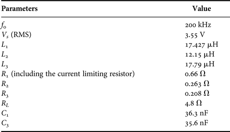
Table 1 shows the practical measured circuit parameters.

Table 1.

The practical system and circuit parameters.

Please note the current limiting resistor is added in the circuit to protect the power amplifier for testing purposes, particularly under fully series tuned conditions which can lead to a very high current. Its resistance is chosen to be very small (making the total ESR of the primary resonant circuit less than 1 Ω) to ensure the normal circuit operation is not much affected. This resistor can be removed in the final system.

In the experiment, the root mean square (RMS) value of input voltage across the resonant circuit of the primary transmitter and the RMS value of the output voltage firstly measured when the power repeater was not added into the system. Then, the power repeater was placed at three different positions which are 40, 80, and 104 mm away from the primary coil, respectively. At each position, the coupling coefficient k ₁₂ between the primary coil and the coil of power repeater and the coupling coefficient k ₂₃ between the coil of power repeater and the pickup coil were measured. By substituting the inductances in Table 1 and the measured k ₁₂, k ₂₃, and k ₁₃ in (16), the mutual inductances M ₁₂, M ₂₃, and M ₁₃ were calculated, respectively for each position. The C _2−Pmax and C _2−Cr for each position were calculated by substituting M ₁₂, M ₂₃, and M ₁₃ and system and circuit parameters in (15) and (11), respectively. Table 2 shows the measured k ₁₂ and k ₂₃, the calculated M ₁₂ and M ₂₃, and the predicted C _2−Pmax and C _2−Cr of the three positions:

(16)$$M = k\sqrt {L_aL_b}, $$

where M is the mutual inductance between two coupled coils, L _a and L _b are the inductances of two coupled coils, respectively, and k is the coupling coefficient between two coupled coils.

Table 2.

The measured coupling coefficients, calculated mutual inductances, predicted critical tuning capacitances, and optimal tuning capacitances for obtaining the maximum output power.

Table 2 shows that C _2−Pmax is smaller than C _2−cr for all three positions. Therefore, the tuning capacitance of the power repeater was manually varied from a tuning capacitance smaller than C _2−Pmax to a tuning capacitance larger than C _2−Cr at each position. Both the RMS values of the output voltage and the input voltages across the resonant circuit of the primary transmitter were measured for all tuning capacitances within the range of the variation.

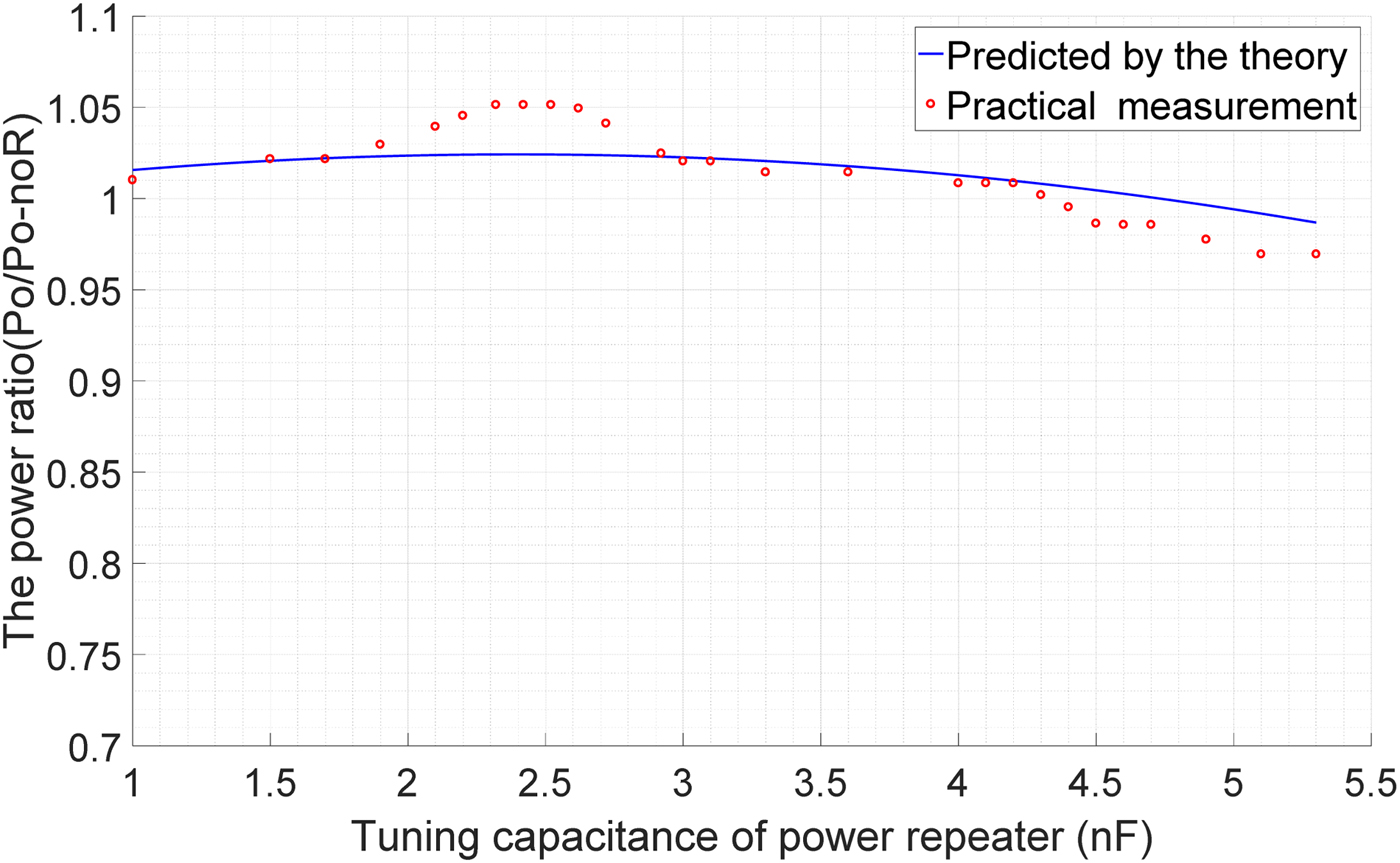
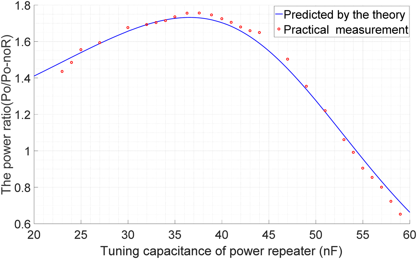
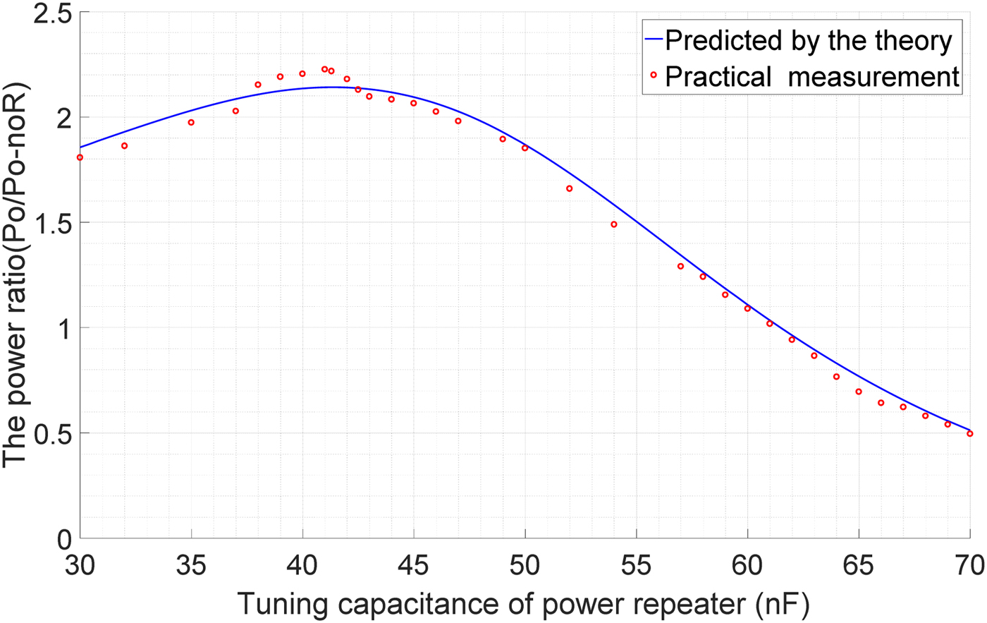
Due to the reflected effects from the passive power repeater and the power pickup, the RMS value of the input voltage from the AC power linear amplifier slightly changed when the tuning capacitance was manually varied. The input voltage was calibrated by dividing 3.55 V which is the input voltage when the power repeater was not added into the system for each measurement. The measured output voltage was calibrated by dividing the ratio between the input voltage and 3.55 V, and the output power was calculated by using the calibrated output voltage. The ratios between the output power of the IPT system with and without the passive power repeater were obtained. Figures 5–7 show measured and predicted output power ratios in relation to the tuning capacitance of the passive power repeater when the passive power repeater was placed at 40, 80, and 104 mm away from the primary coil, respectively.

Fig. 5.

The measured and predicted output power ratios at tuning capacitances within the range between 1 and 5.3 nF when the passive power repeaters is placed 40 mm away from the primary coil.

Fig. 6.

The measured and predicted output power ratios at tuning capacitances within the range between 20 and 60 nF when the passive power repeater is placed 80 mm away from the primary coil.

Fig. 7.

The measured and predicted output power ratios at tuning capacitances within the range between 30 and 70 nF when the passive power repeater is placed 104 mm away from the primary coil.

Figure 5 shows that the measured output power ratios are in good agreement with the predicted power ratios when the passive power repeater was placed 40 mm away from the primacy coil. The maximum measured power ratio of 1.05 was achieved when the tuning capacitance of power repeater is between 2.3 and 2.5 nF, and the predicted tuning capacitance is 2.43 nF which is 5.65% larger than 2.3 nF. The measured critical tuning capacitance for enhancing and reducing the output power is 4.3 nF which is 10% smaller than its predicted value of 4.73 nF.

Figure 6 shows that the measured power ratios are consistent with the predicted power ratios when the passive power repeater was placed 80 mm away from the primary coil. The output power was maximized by around 71.9% at 37.6 nF which is 2.73% larger than the predicted tuning capacitance of 36.6 nF. The measured critical tuning capacitance is 54 nF which is 0.55% smaller than its predicted value of 54.3 nF.

Figure 7 shows that the measured power ratios are in good agreement with the predicted power ratios when the passive power repeater was placed 104 mm away from the primary coil. The output power was maximized by 122% when the tuning capacitance equals to 41 nF which is 1% off from the predicted capacitance of 41.4 nF, and output power ratio is approximately equal to one when the tuning capacitance is 61 nF which is 0.66% smaller than the predicted tuning capacitance of 61.4 nF.

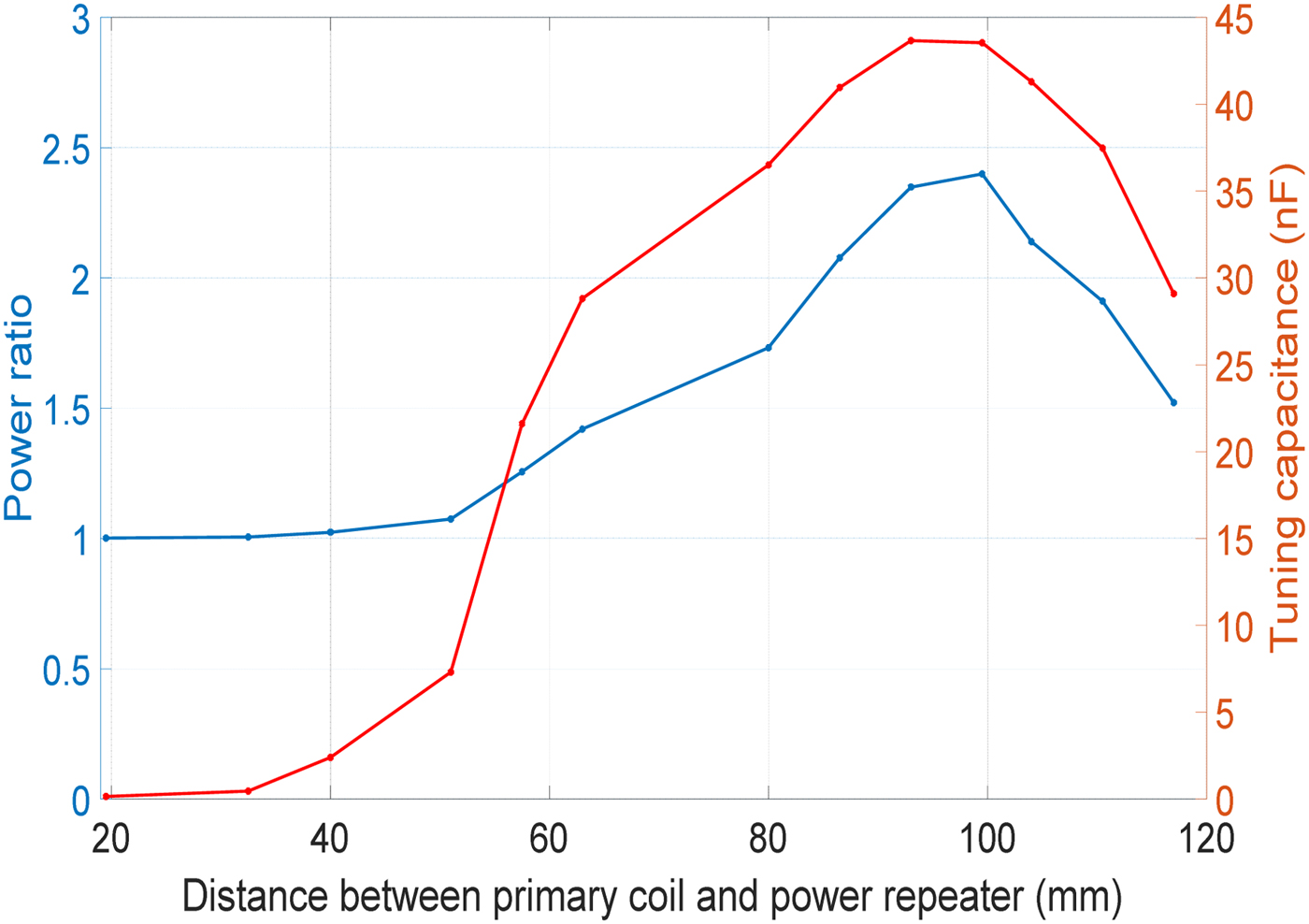
Figures 5–7 show the maximum power transfer ratio changes with the position of the power repeater. The position of a power repeater with a fixed tuning condition has been determined for maximum power transfer efficiency in [Reference Kiani, Jow and Ghovanloo24, Reference Niu, Wang, Chu and Gu25], and the analytical result in relation to the position was obtained by ignoring the mutual inductance between the primary coil and pickup coil. The relationship between the system output power and the position of the power repeater becomes more complicated in the system presented in this paper after considering the mutual inductance between the primary coil and pickup coil. Furthermore, to obtain the maximum power transfer, the tuning capacitance of the power repeater needs to be varied away from the nominal tuning capacitance at different positions of the power repeater. To obtain the relationship between the output power and the position of the power repeater, the mutual inductances M ₁₂ and M ₁₃ at 13 positions between the primary coil and the power repeater are practically measured, then the maximum output power ratios (with respect to the output power without using a power repeater) are calculated for each position, as shown in Fig. 8, together with the tuning capacitance variations.

Fig. 8.

The relationship between the power ratio and distance between the primary coil and power repeater.

It can be seen from Fig. 8 that the maximum output power increases with the increase of the distance between the primary coil and the power repeater until it reaches about 100 mm, and then the output power decreases when the repeater approaches the power pickup. The power ratio reaches the maximum value of about 2.4 when the tuning capacitance of the power repeater is close to 43 nF.