2. DATA SOURCES

This paper combines two methodological and data approaches: social tables from 1850 to 1950 and modern household surveys from 1960 to 2010. These two approaches permit us to obtain direct estimates for income inequality—measured with the Gini index—since they provide a description of the population structure and income distribution. However, while both approaches use pre-tax incomes, their unit of analysis is not fully equivalent. In particular, social tables combine data on the number of people in different classes—occupational groups—and the estimated average incomes linked to them, while modern household surveys offer information on income per person or household instead of groups. For this reason, social tables cannot register as much detail as that reported by modern household surveys such as data on family formation. Therefore, it should be noted that inequality values for periods prior to 1950 based on social tables are subject to a higher measurement error when compared with those coming from household surveys. Nevertheless, in the absence of household surveys or fiscal data, social tables appear as the best source of information on income distribution prior to the 20^th century, and in combination with modern surveys, serve us well to draw long-run inequality trends and allow for the identification of specific patterns such as the Kuznets curve. In what follows, I present details on data and the sources applied for the estimation of inequality at different periods from these two alternative approaches.

I use social tables to measure Brazil's inequality between 1850 and 1950. Traditionally, social tables have been used to estimate inequality in particular benchmark years (Lindert and Williamson Reference Lindert and Williamson1982, Reference Lindert and Williamson1983; Milanovic et al. Reference Milanovic, Lindert and Williamson2010)Footnote ⁴. In order to explore countries' income distribution for longer periods, some authors built dynamic social tables where both population and income shares oscillate annually (Rodríguez Weber Reference Rodríguez Weber, Bértola and Williamson2017; Gómez León and de Jong Reference Gómez León and de Jong2019)Footnote ⁵. Unfortunately, the construction of dynamic social tables (which interpolate population between census benchmark years) is not feasible for the case of Brazil. This is because of the long periods between censuses (the census of 1872 was only followed by the one in 1920) and the significant changes in the occupational structure after the abolition of slavery (in 1888)Footnote ⁶. Hence, as a midway approach, I take the population structures reported in the population censuses as fixed, while associated incomes fluctuate annually (Bértola et al. Reference Bértola, Castelnovo, Reis and Willebald2007; Gómez León Reference Gómez León2019). Therefore, for the period 1850-1898, I use the census of 1872; from 1899 to 1930, the 1920 census; and for 1940 and 1950, the censuses carried out in those years.

Annual income data for each professional category has been compiled from different sources: censuses (Diretoria Geral de Estatística, 1872; 1926; 1950; 1956), Historical Statistics (Instituto Brasileiro de Geografía e Estatística, 1990) and official information on nominal wages provided by Lobo (Reference Lobo1978). The latter, already used by Arroyo Abad and Astorga (Reference Arroyo Abad and Astorga2017) and Gómez León (Reference Gómez León2019), while mostly reflecting living standards in Rio de Janeiro, represents the only available source to capture income differences across a comprehensive number of occupational groups for a long span of time in BrazilFootnote ⁷. Since these data limitations are likely to underestimate inequality levels, when possible, nominal wages from Lobo have been adjusted with municipal data on the list of voters, associated wages and occupations (Klein Reference Klein1995; Nunes Reference Nunes2003; Monasterio Reference Monasterio2010) and with national official censuses (Diretoria Geral de Estatística, 1872; 1895; 1926; 1950; 1956)Footnote ⁸. Additional data on landowners and slaves come from unpublished work by Henry Willebald and Leonardo Monasterio. See Data Appendix for details.

It should also be noted that social tables in general have the limitation of assuming equal average income per social class, thus neglecting potential variation within groups. Thus, potential inequalities within groups should be considered by introducing as much disaggregation within professional groups as possible. In this case, Brazil's censuses allow for distinctions to be made by gender (male and female) and condition (free and slave) within each occupational category (across agriculture, industry and services sectors). Meanwhile income data disaggregated by social characteristics (gender and condition) are obtained from a range of sources and estimated under conservative assumptions. For instance, there is evidence that females' earnings in industry were 60 per cent of male earnings according to the information provided by the census of 1920 (Diretoria Geral de Estatística 1926). Likewise, municipal data from Klein (Reference Klein1995), Nunes (Reference Nunes2003) and Monasterio (Reference Monasterio2010) permit us to infer the distribution of workers in urban and rural areas and their relative income differencesFootnote ⁹.

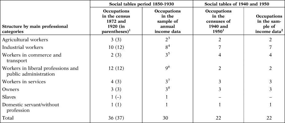
Despite the abovementioned limitations, the resulting social tables offer a broad description of Brazil's population and income distribution across seven main work categories detailed in Table 1. The main difference between the periods of 1850-1930 and 1940 and 1950 is the reduction of occupations from 36 to 22Footnote ¹⁰. This is due to the absence of more disaggregated data for the category of liberal professions and public administration in the censuses of 1940 and 1950. As discussed above, a smaller sample of groups leads to minimising the internal dispersion of this particular professional group, which might, in turn, result in the underestimation of total inequality in 1940 and 1950. Nevertheless, the inclusion of a higher number of occupations within this category would contribute to reinforcing, but not to modifying, rising inequality trends between 1930 and 1950, which, as discussed in Sections 4 and 5, is mostly driven by an increasing concentration of income in the top part of the distribution.

TABLE 1

NUMBER OF OCCUPATIONS IN THE CENSUSES AND IN THE SAMPLE OF INCOMES BY PERIOD

Source: See Tables A1.1 and A1.2 in the Appendix.

¹ Occupations in the censuses of 1872 and 1920 can be found in Tables A1.1 and A1.2 of the Data Appendix.

² Occupations in the sample of income data for 1940 and 1950 coincide with those appearing in the census.

³ Horticulturist journey man.

⁴ Blacksmith, carpenter, construction worker, dressmaker, distiller, machine worker, press workers and miner.

⁵ Retailer, chemist and machine worker.

⁶ Doctor, government administrator, judge, lawyer, nun, priest, sexton, surgeon and teacher.

⁷ Artist, domestic services and nurse.

⁸ Agriculture, industry and services.

Inequality estimates after 1950 (computed from direct access to nationally representative household surveys) have been taken from All the Ginis dataset (ALG)Footnote ¹¹. For the case of Brazil, the ALG combines and homogenises information from individual studies (Ferreira et al. Reference Ferreira, Leite and Litchfield2008, Table 1) and three different datasets (LIS, SEDLAD and WIDER)Footnote ¹².

3. REVISITING BRAZIL'S HISTORICAL INEQUALITY

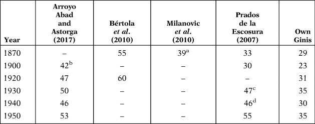
Existing quantitative studies of Brazil's historical inequality before 1950 (measured as Gini coefficients) illustrate two alternative evolutions of Brazilian income distribution (Table 2)Footnote ¹³. On the one hand, benchmark estimations based on social tables from Bértola et al. (Reference Bértola, Castelnovo, Rodríguez and Willebald2010) show a Gini close to 55 as early as 1870 that continued to increase during the 20^th century. On the other, the Gini obtained from social tables by Milanovic et al. (Reference Milanovic, Lindert and Williamson2010) and the so-called pseudo-Ginis estimated by Prados de la Escosura (Reference Prados De La Escosura, Hatton, O'Rourke and Taylor2007) report lower inequality levels for 1870Footnote ¹⁴. Similarly, computations on Brazil's inequality across occupational groups by Arroyo Abad and Astorga (Reference Arroyo Abad and Astorga2017) show a Gini of 42 as late as 1900. Crucially, this second view questions the notion of persistent high inequality levels in Brazil, which would have started to increase from the 20^th century.

TABLE 2

BRAZIL'S INEQUALITY ESTIMATES (1870-1950)

Sources: Arroyo Abad and Astorga (Reference Arroyo Abad and Astorga2017), Bértola et al. (Reference Bértola, Castelnovo, Rodríguez and Willebald2010), Milanovic et al. (Reference Milanovic, Lindert and Williamson2010) and Prados de la Escosura (Reference Prados De La Escosura, Hatton, O'Rourke and Taylor2007).

Notes: Original estimations are in years: ^a1872, ^b1902, ^c1929 and ^d1938. This table summarises Brazil's inequality estimates for matching benchmark years. For the complete series on pseudo-Ginis, see Prados de la Escosura (Reference Prados De La Escosura, Hatton, O'Rourke and Taylor2007). Arroyo Abad and Astorga (Reference Arroyo Abad and Astorga2017) also provide series on inequality between occupational groups between 1902 and 1950.

Evidence from the Ginis developed in this paper supports this line by showing increasing inequality trends from 1900 onwards. My lower values might be linked to limited information on income dispersion within occupational groups as well as on property incomes. That is, the underestimation of the internal dispersion within groups is likely to reduce inequality levels. Yet, there is evidence that in very stratified societies, such as Brazil during 19^th century, inequality trends tend to be mostly driven by differences between groups (Milanovic et al. Reference Milanovic, Lindert and Williamson2010, p. 259)Footnote ¹⁵. Moreover, since wealth is disproportionally concentrated among the richest, the undervaluation of property incomes also tends to reduce inequality values. However, it does not necessarily affect trends. In particular, for the case of Brazil, Arroyo Abad and Astorga (Reference Arroyo Abad and Astorga2017, p. 361) found that inequality trends when including property incomes in the top part of the distribution moved in line with those considering labour incomes onlyFootnote ¹⁶. This supports the plausibility of Brazil's inequality trends obtained from social tables.

Additionally, the estimation of a lack of persistent high inequality in Brazil finds additional support in the Inequality Possibility Frontier concept developed by Milanovic (Reference Milanovic2006), who theorised about the existence of a maximum attainable inequality that increases with mean overall incomeFootnote ¹⁷. In this sense, there is evidence that increasing inequality values in Brazil for the first half of the 20^th century went along with increasing mean incomes and decreasing extraction ratios Footnote ¹⁸. Nonetheless, Brazil's recent experience for the early 21^st century suggests a picture of increasing mean incomes along with decreasing inequality and poverty reduction (Côrtes Neri Reference Côrtes Neri2010; Ferreira et al. Reference Ferreira, Messina, Rigolini, López Calva, Lugo and Vakis2013). These different patterns can be further discussed by exploring the existence and completion of a Kuznets curve.

4. VALIDATING KUZNETS’ HYPOTHESIS

Since Kuznets' (Reference Kuznets1955) seminal article on Economic growth and income inequality, interest in the relationship between processes of development and distribution of income has rapidly flourished, with a large part of the debate centred on testing the inverted-U relationship conjectured by Kuznets. There are two phases in the transition from a pre-industrial society to a post-industrial one that help to explain this shape. The initial upward trend is explained by the transference of labour from a low productive and relatively egalitarian agricultural sector to a higher productive and more unequal industrial sector, along with the increasing migration to the cities from the countryside and, thus, by a growing weight of a more inegalitarian urban population. The downward part takes place with the completion of this transference and with growing political power of urban masses demanding more protective legislation, progressive taxation and developed welfare systems.

When testing this hypothesis empirically, some authors validated the inverted-U relationship for developed countries (van Zanden Reference van Zanden1995; Williamson Reference Williamson2010), while the evidence for developing countries is more ambiguous (Ahluwalia Reference Ahluwalia1976; Anand and Kanbur Reference Anand and Kanbur1993; Deininger and Squire Reference Deininger and Squire1998; Kanbur Reference Kanbur and Kochhar2011)Footnote ¹⁹. Notably, most empirical investigation of the relationship between development and inequality has been based on cross-country data. In this sense, Ahluwalia (Reference Ahluwalia1976) and Kanbur (Reference Kanbur and Kochhar2011) agree that dynamic processes, such as those hypothesised in Kuznets (Reference Kuznets1955), should be examined and confirmed in explicit historical contexts and for particular countries. The contribution by Prados de la Escosura (Reference Prados De La Escosura2008) on the investigation of the Kuznets curve in Spain between 1850 and 2000 is a good example. For Latin American countries, we can find some discussion for the cases of Argentina and Uruguay (Bértola Reference Bértola2005), and for Brazil and Chile (Milanovic Reference Milanovic2016). However, to test this hypothesis more rigorously, I test the presence of the Kuznets curve in Brazil with regression analysis (Ahluwalia Reference Ahluwalia1976; Deininger and Squire Reference Deininger and Squire1998; Barro Reference Barro2000; Williamson Reference Williamson2010; Milanovic Reference Milanovic2018), as well as on the basis of inequality time series and on the evolution of inequality against contemporary values of GDP per capita (Prados de la Escosura Reference Prados De La Escosura2008; Milanovic Reference Milanovic2016).

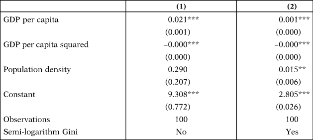
In Table 3, I use OLS regressions with Gini as the dependent variable, and this is explained by GDP per capita (as a measure of national development), the square of GDP per capita (to test the existence of an inverted relationship), population density (as an additional control) and an error termFootnote ²⁰. Essentially, if a Kuznets curve exists, one would expect GDP per capita to be positive and its square to be negative with both measures being statistically significant. Results in Table 3 (column 1) are supportive of the existence of a Kuznets curve in Brazil. GDP per capita is positive and statistically significant (0.021; 95 per cent CI: from 0.019 to 0.022) and its quadratic form displays the expected negative sign and is also statistically significant (−0.000; 95 per cent CI: from −0.001 to −0.000)Footnote ²¹. Population density displays a positive sign, but it is not statistically significant once controlling for per capita GDP (0.290; 95 per cent CI: from −0.121 to 0.701). Its positive sign can be explained in a Lewis (Reference Lewis1954) model context where a surplus of labour from the countryside permitted the more productive sector to absorb a growing urban labour force while maintaining wages at subsistence levels, thus, widening the gap between owners and workers and, thus, increasing inequality. The baseline results are robust to a semi-logarithm transformation (column 2) with all variables maintaining their respective signs while showing higher significance levels (1 per cent level for GDP and its quadratic form, and 5 per cent level for population density)Footnote ²².

TABLE 3

INEQUALITY-DEVELOPMENT RELATIONSHIP IN BRAZIL, 1850-2010

Source: For inequality data see text.

Notes: GDP per capita data are from Maddison Project Database 2013. Population density was computed as population (in thousands) from Maddison Project Database 2013 divided by Brazil's current area (in km²). The semi-logarithm Gini is calculated as f(logs). Missing years in the data are due to a lack of Gini data. Robust standard errors are in parentheses, ***P < 0.01, **P < 0.05, *P < 0.1.

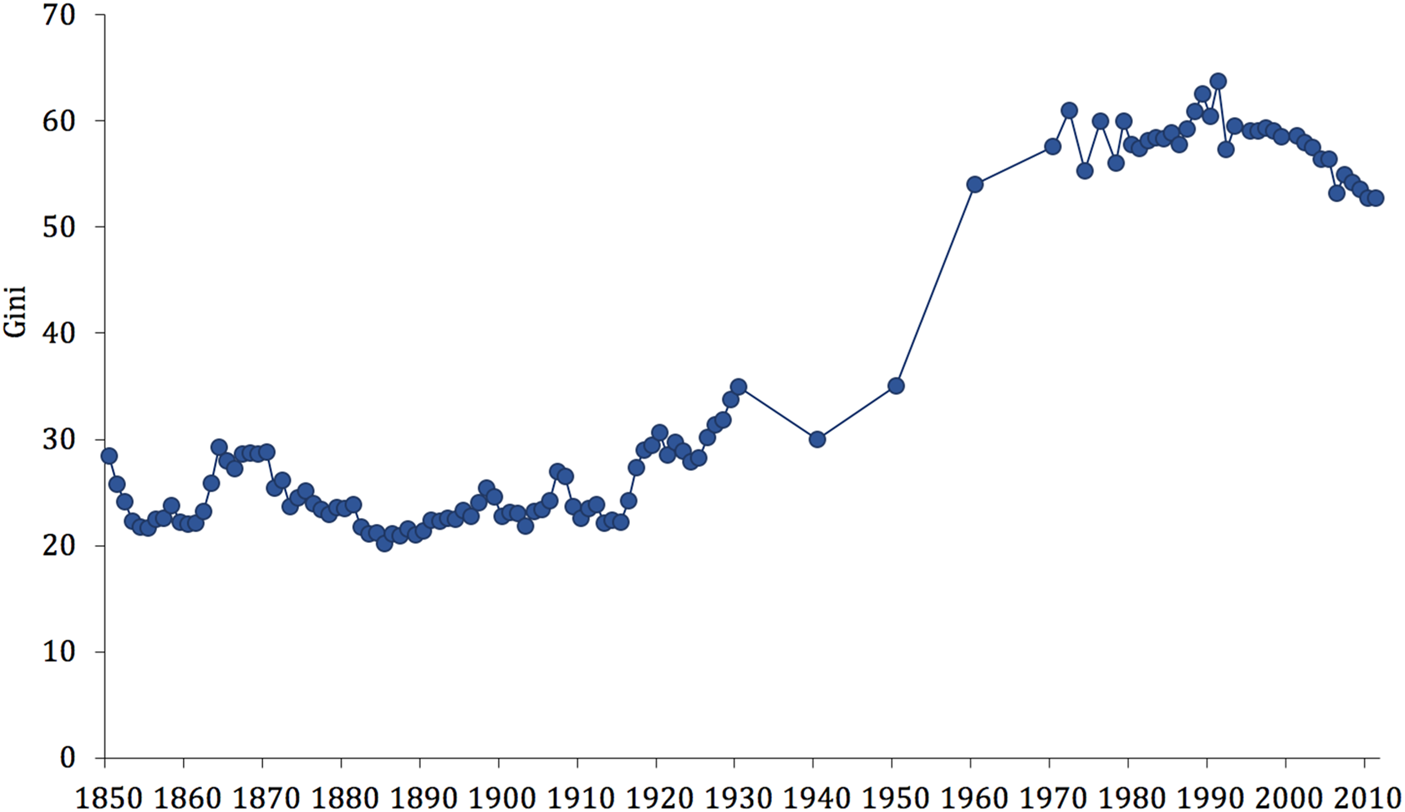
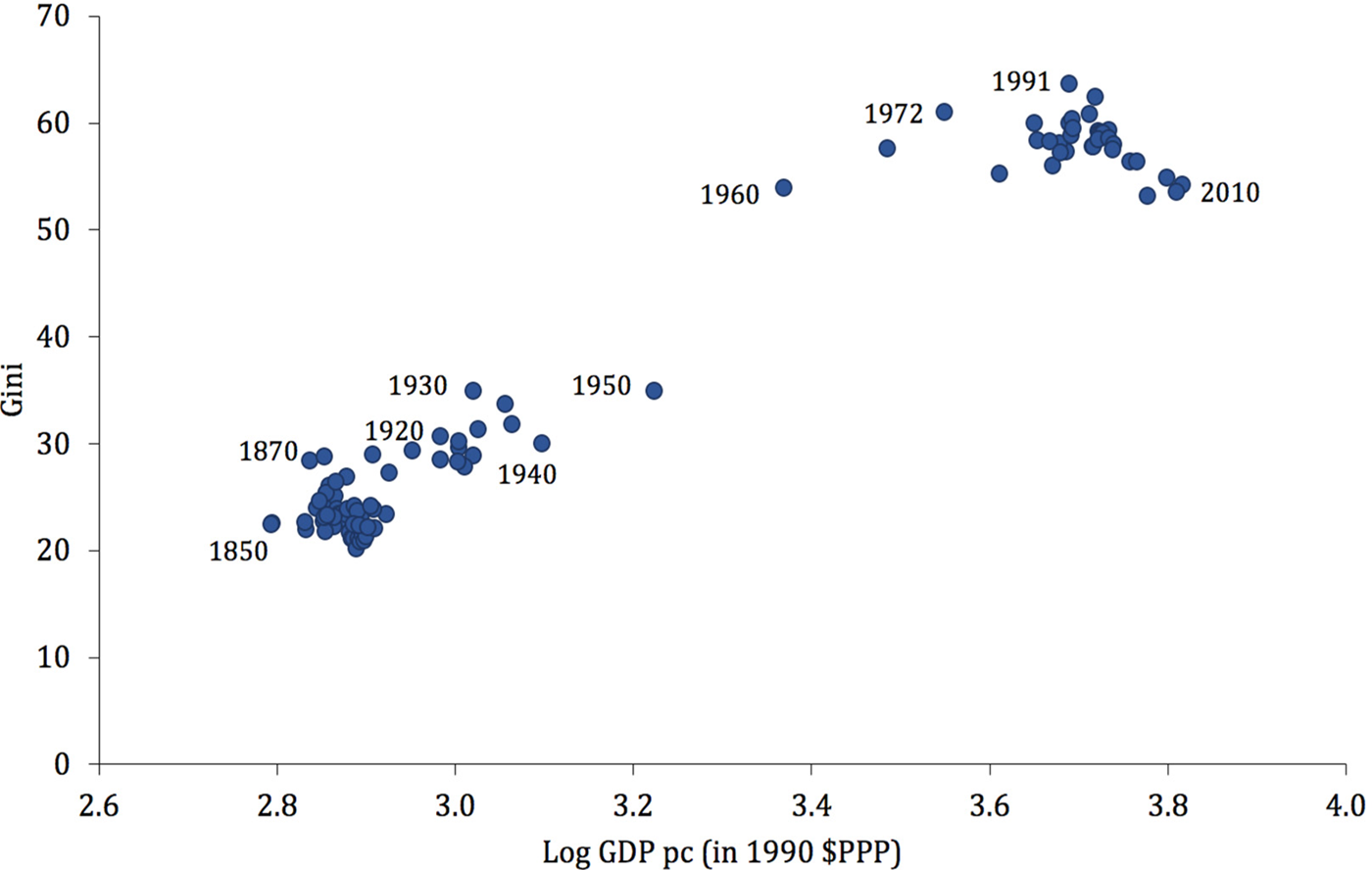
Next, in Figures 1 and 2, I show the evolution of inequality across time and against contemporary GDP per capitaFootnote ²³. In both cases it is possible to observe a curve pattern with increasing inequality from the late 19^th century, remaining at a high plateau between the 1970s and 1990s, and declining afterwards. The long-term shape (1850-2010) coincides with that suggested in Milanovic (Reference Milanovic2016, p. 82). Meanwhile, short-term trajectories are in line with those observed by Prados de la Escosura (Reference Prados De La Escosura, Hatton, O'Rourke and Taylor2007) and Arroyo Abad and Astorga (Reference Arroyo Abad and Astorga2017), showing increasing inequality between 1900 and 1950.

FIGURE 1

THE DEVELOPMENT OF THE GINI INDEX IN BRAZIL, 1850-2010.

Sources: From 1850-1950 Gini estimates obtained from social tables; from 1960 to 2010 Gini estimates from All the Ginis (ALG) Dataset. GDP per capita from Maddison Project Database 2013.Notes: Gini coefficients expressed in percentages.

FIGURE 2

GINI VS. GDP PER CAPITA (IN NATURAL LOGARITHMS) IN BRAZIL, 1850-2010.

Sources: From 1850-1950 Gini estimates obtained from social tables; from 1960 to 2010 Gini estimates from All the Ginis (ALG) Dataset. GDP per capita from Maddison Project Database 2013.Notes: Gini coefficients expressed in percentages.

Interestingly, in both figures, the concave shape supports the hypothesis, as advanced in Section 3, that low inequality values during the 19^th century were linked to low income levels associated with an essentially rural society, which prevented the Kuznets curve from taking offFootnote ²⁴. The rise in inequality, starting from the early 20^th century, came along with increasing GDP per capita. During this period, the boom of coffee exports as well as new investments and initiatives in favour of industry created a favourable economic climateFootnote ²⁵. Meanwhile, people who had previously arrived from Europe and Asia to fill Brazil's coffee fields and the internal migrants from poorer north-eastern regions moved to the expanding urban cities in the south-east (Lobo Reference Lobo1978, p. 469; Goldsmith Reference Goldsmith1986, p. 146; Luna and Klein Reference Luna and Klein2006, p. 172). Therefore, both economic and social factors suggest that the increase in inequality during the early 20^th century was linked to a process of modernisation and urbanisation, which converged on the emergence of an urban middle class (Iglesias Reference Iglesias1994, p. 33; Owensby Reference Owensby1999, p. 132; Gómez León Reference Gómez León2019, p. 493).

From the beginning of the ISI era (in the 1930s), both inequality and GDP per capita continued to increaseFootnote ²⁶. During this period, the industrial sector became the engine of Brazil's economic growth while the process of urbanisation, especially after WWII, accelerated (Goldsmith Reference Goldsmith1986; Luna and Klein 2006)Footnote ²⁷. However, the state control under Vargas' Estado Novo (1930-1945) also involved the implementation of co-opted unions and the repression of labour movements (Skidmore Reference Skidmore1967, p. 40; Chacón Reference Chacón1977, p. 56; Luna and Klein Reference Luna and Klein2014, p. 10). In this sense, increasing inequality during this period might be explained by the aforementioned Lewis (Reference Lewis1954) model, where a more elastic supply of labour, in tandem with authoritarian industrial relation policies, ensured high industrial profits at low labour costs (Wolfe Reference Wolfe1993, pp. 89-90)Footnote ²⁸.

Despite the lack of annual data on income distribution, the results based on benchmark estimates suggest that the relationship between GDP per head and inequality remained positive between the 1950s and 1970s. These were Brazil's ISI golden years, when the economy grew at an annual rate of 8.2 per cent (Luna and Klein Reference Luna and Klein2006, p. 138). However, during this time the fast-growing labour force contributed to wage gaps between workers, under-unemployment and an unequal distribution of the benefits of this growth (Bulmer-Thomas Reference Bulmer-Thomas2003, p. 307). Political factors also played an important role during this period. According to Frankema (Reference Frankema2010, p. 363), when urban labour force growth accelerated, the internal stability of labour unions was undermined and much of the political attention focused on the trade-off between formal wage levels and employment creationFootnote ²⁹. Following the military coup of 1964, sharp reductions in real wages, the prosecution of worker movements, and the concentration of income in the upper deciles all contributed to worsen Brazil's income distribution (Morley Reference Morley2001, p. 113; Bulmer-Thomas Reference Bulmer-Thomas2003, p. 316; Luna and Klein Reference Luna and Klein2006, p. 17).

In the 1980s, during the so-called «lost decade», Brazil reached a plateau of stagnant GDP per head and high inequality levels. This decade was marked both politically by the path to democracy (Mainwaring Reference Mainwaring1986), and economically by the transference from a traditional interventionist development model to a liberalisation process (Luna and Klein Reference Luna and Klein2006)Footnote ³⁰. During these years, foreign debt and especially high inflation destabilised Brazil's economy with a regressive impact on the income distribution, with the poor suffering particularly (Bulmer-Thomas Reference Bulmer-Thomas2003, p. 404; Ferreira et al. Reference Ferreira, Leite and Litchfield2008, p. 24)Footnote ³¹. Yet, after peaking in 1990, Brazil's inequality reached a turning point. From this point on, Brazil seems to have started a downward Kuznets curve phase, wherein economic growth and declining inequality went hand-in-hand. Potential explanations for the timing and drivers of such a reversal are discussed in the following section.

5. BRAZIL'S ECONOMIC GROWTH DISTRIBUTION

What was behind the reversion of the Kuznets curve? Why did it not take place during earlier years of economic growth? The hypothesis suggested here, as conjectured by Kuznets (Reference Kuznets1955, p. 24), points towards the importance of political initiatives that help to promote economic growth while alleviating the potential dislocating effects associated with it (thus creating opportunities for more vulnerable groups)Footnote ³². In this sense, there is evidence to suggest that the turning point (in the 1990s) matches a period in which both market-oriented reforms as well as distribution policies started to be implemented in Brazil (Ferreira et al. Reference Ferreira, Leite and Litchfield2008; Barros et al. Reference Barros, Carvalho, Franco, Mendoça, López Calva and Lustig2010; Gasparini et al. Reference Gasparini, Cruces, Tornarolli and Mejía2011). This strategy made it possible to reduce inequalities and absolute poverty and increase the size of a new middle classFootnote ³³.

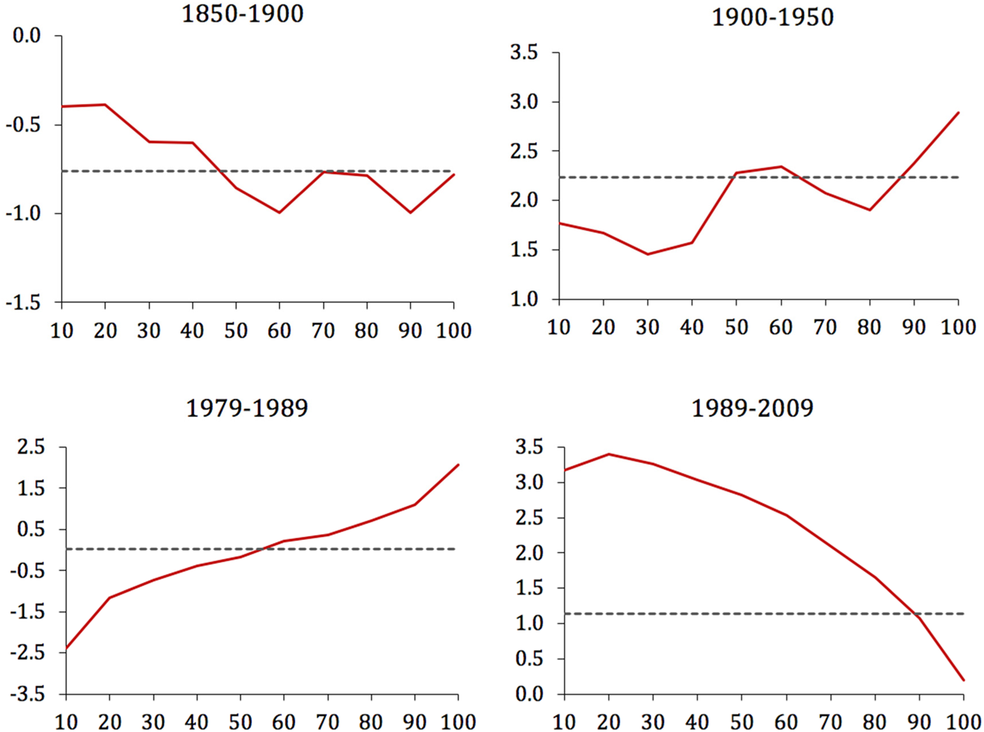
Looking at how economic growth was distributed in Brazil at different periods might help to validate this hypothesis. In this regard, the construction of growth incidences curves (GICs), introduced by Ravallion and Chen (Reference Ravallion and Chen2003) and extensively used by other scholars (e.g. Ferreira et al. Reference Ferreira, Messina, Rigolini, López Calva, Lugo and Vakis2013; Lakner and Milanovic Reference Lakner and Milanovic2013; Milanovic Reference Milanovic2016), can shed new light. Essentially, GICs display compound growth rates in average real incomes for particular parts of the distribution between two benchmark yearsFootnote ³⁴. In so doing, they show how periods of economic expansion or economic downturn affect different segments of the populationFootnote ³⁵. An upward trend suggests that the highest part of the distribution benefitted relatively more during a specific period (and thus represents an increase in inequality), while a downward trend suggests the opposite. Figure 3 shows GICs for Brazil in four main periods: 1850-1900; 1900-1950; 1979-1989 and 1989-2009. The y-axes show average annual compound growth rates in real incomes (expressed in percentages) between benchmark yearsFootnote ³⁶. The x-axes plot deciles of Brazil's income distribution.

FIGURE 3

BRAZIL'S INCOME GROWTH DISTRIBUTION.

Source: See Section 2.Notes: The y-axes show average annual compound growth rates of real incomes (expressed in per cent) at different percentiles of the distribution (drawn on the x-axes) between two benchmark years. Solid red lines show GICs. The straight dashed lines show overall average annual growth rates of real incomes.

Between 1850 and 1900, mean real incomes fell, while losses were similar across the distribution (around −0.8 per cent); the lower 50 per cent being slightly less affected than the rest. During this period, structural changes, including the abolition of slavery and the arrival of European immigration (Leff Reference Leff1982, pp. 52-53; Iglesias Reference Iglesias1994, p. 12; Sánchez Alonso Reference Sánchez Alonso2007, p. 406), together with a deceleration of the economy (Leff Reference Leff1982, p. 84; Goldsmith Reference Goldsmith1986, p. 90), helped the deconcentration of incomes (Gómez León Reference Gómez León2019, p. 489)Footnote ³⁷. The fall in inequality during this period seems to be linked to the stagnation or even decline of salaries in industry, commerce, public administration and liberal professions (placed above the 50th percentile). Importantly, low inequality levels linked to a context of economic deceleration and moderate social mobility prospects prevented a Kuznets curve from taking off during this period.

Next, between 1900 and 1950, real incomes increased for the entire distribution, while biggest gains were recorded for the top 50 per cent. This occurred during a period of increasing urbanisation, development of industry and spread of education (Goldsmith Reference Goldsmith1986, p. 246; Iglesias Reference Iglesias1994, p. 63; Stolz et al. Reference Stolz, Baten and Botelho2013, p. 112). Increasing inequality (as suggested by the upward GIC trend) during this period might be explained as a result of an early development phase where the transition to better remunerated sectors brought benefits to those who could benefit from this process and access new jobs. The process of industrialisation and urbanisation led to the emergence of new professions in both industrial and service sectors (Furtado Reference Furtado1965, p. 14; Wolfe Reference Wolfe1993, pp. 6-7; Owensby Reference Owensby1999, p. 49). Crucially, the increasing demand for skilled workers in manual and non-manual industrial sectors translated into higher wages in these professions (placed above the 50th percentile). For instance, during this period wages of operators in chemical plants became nearly 40 per cent higher than the average in industry, while nominal incomes of those employed in liberal professions and the civil services went up by a factor of five.

While I lack detailed information on income distribution to draw the GICs for the period between 1950s and 1970s, evidence on the evolution of the top 1 per cent income share suggests increasing inequality during this period, accelerating after the military coup of 1964 (Souza and Medeiros Reference Souza and Medeiros2015, pp. 127-129, Figure 3)Footnote ³⁸. Likewise, GICs between 1979 and 1989 suggest that during the following decade, most of it still under the military regime and in a context of economic recession, only the richest 10 per cent registered real income gains above 1 per cent annually. The crisis which mostly hit those below the 50th percentile was particularly suffered by the bottom 20 per cent. During this period, macroeconomic instability made the fight against inflation and fiscal fragility the highest priorities, while leaving development off the political agenda (Moreira Cunha and da Silva Bichara Reference Moreira Cunha and da Silva Bichara2004, p. 40; Luna and Klein Reference Luna and Klein2006, p. 141). Meanwhile, skill-biased technological change, together with the erosion of the bargaining power of labour vs. management, contributed to rising interpersonal income inequalities (Morley Reference Morley2001, p. 113; Frankema Reference Frankema2009, p. 146).

Finally, between 1990 and 2009, already in democracy and in a context of increasing real incomes for the entire distribution, the top 10 per cent was the only population segment registering gains below the average. Notably, the downward GIC trend during this period suggests decreasing inequality, with a pro-poor economic growth (wherein the bottom 50 per cent registered annual growth rates in real incomes above 3 per cent). During the 1990s, the introduction of market-oriented reforms (including the reduction of import tariffs, the privatisation of state industries and public services, and currency changes) put an end to the existing interventionist economic system and opened local markets to international competition and globalisation (Bulmer-Thomas Reference Bulmer-Thomas2003; Luna and Klein Reference Luna and Klein2006; Frankema Reference Frankema2009). As discussed, trade openness might have played an important role in Brazil's income distribution. Scholars including Luna and Klein (Reference Luna and Klein2006) and Morley (Reference Morley2001) found that the disappearance of some industries and the exposure of local producers to external competitors had adverse effects on employmentFootnote ³⁹. Others have highlighted positive outcomes through the reduction of wage gaps in industry (Gonzaga et al. Reference Gonzaga, Menezes Filho and Terra2008) and the convergence of rural and urban incomes sectors (Ferreira et al. Reference Ferreira, Leite and Litchfield2008). A broader consensus can be found on the equalising effects of the introduction of redistributive policies, which allowed for a new middle-class emergence and the reduction of poverty (Côrtes Neri Reference Côrtes Neri2010; Cacciamali Reference Cacciamali2011; Ferreira et al. Reference Ferreira, Messina, Rigolini, López Calva, Lugo and Vakis2013; Arnold and Jalles Reference Arnold and Jalles2014).

On the above point, some of the redistributive initiatives involved labour market policies (including the active regulation of minimum wages and the extension of unemployment insurance), subsidised credits through micro-bank systems and income transfers aimed at assisting more vulnerable groups (children, elderly people and those in the poorest rural areas). Notably, the introduction of economic policies that aimed at enhancing efficiency and growth in combination with distributive policies (that alleviate the potential desequalising effects of this growth) might have allowed for a turning point in Brazil's trajectory, initiating a second phase of economic development along with decreasing inequality.

Yet, a new step back in inequality reduction following the global financial crisis in 2008 is reflected by a growing concentration of income in the top decile (Alvaredo et al. Reference Alvaredo, Chancel, Piketty, Saez and Zucman2018). In this vein, Souza and Medeiros (Reference Souza and Medeiros2015) find that the apparent decline in the Gini coefficient, recorded by surveys in 2006-2012, vanishes once adjusted for the underestimation of top incomes. Therefore, trends in top incomes might have mitigated changes in the bottom part of the distribution. This suggests that in order to enable the completion of the Kuznets curve, previous initiatives addressing the reduction of labour-income disparities should also be complemented with policies aimed at reducing non-labour income inequalities, for instance, by means of more progressive tax policies or the deconcentration of capital ownership (Milanovic Reference Milanovic2019; Saez and Zucman Reference Saez and Zucman2019).

6. CONCLUDING REMARKS

Combining a new dataset on Brazil's income distribution based on social tables with modern inequality estimations obtained from household surveys, this paper has examined Brazil's historical inequality between 1850 and 2010 and tested the presence of a Kuznets curve during this historical period. In this way, it has brought together an old debate about the persistence of inequality in Latin American countries and a vivid discussion of the relationship between development and income distribution.

The paper's results are in line with those of Arroyo Abad and Astorga (Reference Arroyo Abad and Astorga2017), Prados de la Escosura (Reference Prados De La Escosura, Hatton, O'Rourke and Taylor2007) and Williamson (Reference Williamson2010) and find little support for the idea of persistent high inequality in Brazil. They also validate the presence of a long Kuznets curve. Brazil's experience seems to conform Kuznets' (Reference Kuznets1955) hypothesis on inequality performance during periods of development, with increasing inequality from the early 20^th century—given a context of modernisation, industrial development and growing urbanisation. Likewise, declining inequality from the 1990s supports Kuznets' conjectures on the potential implications for developing countries of initiating political practices that foster economic growth, while enhancing the position of the lower-income groups, so as to accomplish the downward part of the curve. In this vein, this paper's thesis points towards both economic and political factors as crucial drivers of inequality changes in Brazil.

Regardless of potential coincidences with well-established theories on the relationship between development and income distribution and shared characteristics with other countries in the region, this investigation is, however, cautious regarding the assumption of a common path for Latin AmericaFootnote ⁴⁰. On the contrary, given the varied nature of the economic and political changes across the region, it suggests the need for further research using individual in-depth study cases (Rodríguez Weber Reference Rodríguez Weber, Bértola and Williamson2017; Gómez León Reference Gómez León2019). Notably, the construction and analysis of detailed particular income distributions would aid the identification of important drivers of inequality and their relationship with individual domestic conditions. Most importantly, by understanding its historical path, present-day policies could serve as prescriptions to avoid recursive misfortunes.