Nomenclature

b

model coefficient

CSA

cuckoo search algorithm

ECAC

European civil aviation conference

f

frequency

ICAO

international civil aviation organization

MAPE

mean absolute percentage error

$\textrm{p}_{\textrm{a}}$

switching factor

PSO

particle swarm optimization

R

correlation coefficient

s

step size

SPL

sound pressure level

Greek symbols

$\alpha$

step size scaling factor

$\Gamma$

constant given for Lévy flight parameter

$\lambda$

Lévy flight parameter

$\otimes$

entry-wise product

$\chi$

constriction coefficient

2.0 Dataset

To estimate the noise produced by a high-performance aircraft, PSO and CSA models were developed using measured F-22A jet noise data at afterburner, published by Neilsen et al. [Reference Neilsen, Gee, Wall and James38].

In this study, noise measured data in the vicinity of a F22-A Raptor, obtained by Neilsen et al., is used to develop two unique metaheuristic models in order to estimate the mixing noise from fine-scale and large-scale turbulent structures. F22-A Raptor is a military aircraft equipped with two F119-PW100 turbofan engines.

A total of 50 ground-based microphones were positioned at various angles, spaced 0.61 meters (2 feet) apart, and aligned parallel to the engine’s centreline at a sideline distance of 11.6 meters (approximately 38 feet). The angles and distances of the source receiver were calculated relative to the engine inlet and an origin positioned 5.5 meters (approximately 8 to 10 nozzle diameters) downstream from the jet nozzle exit. The F-22A aircraft generally operates in four different engine power settings: idle, intermediate power, military power and afterburner [Reference Tam and Parrish25]. Military power refers to the maximum power the engine can deliver without afterburner. With afterburner, the engine power percentage varies depending on the engine type used. The engine closest to the measurement microphones was operated under three power conditions: full afterburner, military power (100%), intermediate level (80%), and while the other engine was kept at idle. In this modeling study, these military noise data obtained at various microphone angles under afterburner power conditions were taken into consideration.

The data obtained from Neilsen et al. were processed through several stages to make it suitable for analysis, and a dataset was prepared. First, the data were transformed into the narrow band (expressed in dB per Hz) to eliminate the excessive emphasis on high-frequency components shown in the 1/3 octave spectra. It was assumed that the noise level remained relatively constant across each 1/3 octave band. In this regard, the following conversion formula can be easily derived in the 1/3 octave spectra:

(1) \begin{align}{\rm{SPL}}\left( {{\rm{per\;Hz\;in\;dB}}} \right) = {\rm{SPL}}\left( {{\rm{1/3\;octave\;band\;in\;dB}}} \right){\rm{-10\;log }}\left( {{\rm{0}}{\rm{.2315\;fc}}} \right)\end{align}

The centre frequency in Hz is expressed as fc.

Next, the SPL was modified as though each data point were recorded at the same distance from the perceived centre of the noise source. The dataset became ready for directivity analysis after this adjustment.

3.0 Metaheuristic methods

3.1 CSA

CSA, introduced in 2009, is a population-based metaheuristic optimisation method that has been extensively employed in a wide range of optimisation tasks due to its straightforward structure, high efficiency and flexibility. A notable advantage of CSA over many other metaheuristic techniques is its independence from gradient information, which makes it especially well-suited for solving non-differentiable and noisy optimisation problems [Reference Yang39–Reference Yang and Deb41].

The CSA uses two search strategies as local and global random walk. The balance between these walks is provided by a switching parameter p_a.

The local random walk is shown in the following equation:

(2) \begin{align}{\rm{x}}_{\rm{i}}^{{\rm{t}} + {\rm{1}}} = {\rm{x}}_{\rm{i}}^{\rm{t}} + \alpha s \otimes H({p_a} - \in ) \otimes (x_j^t - x_k^t)\end{align}

where x_i ^t and x_i ^t+1 represent the current and next solutions, respectively. The variable s is the step size, while α is the step size scaling factor. ⊗ denotes entry-wise product, and H(u) indicates the heaviside function. Finally the term is a random number drawn from a uniform distribution.

The global random walk is based on Levy flight is represented by

(3) \begin{align}{\rm{x}}_{\rm{i}}^{{\rm{t}} + {\rm{1}}} = {\rm{x}}_{\rm{i}}^{\rm{t}} + \alpha L(s,\lambda )\end{align}

where $L(s,\lambda )$ denotes the Levy distribution. This parameter specifies the random step length and thus allows the solution to be searched in a more detailed and wider range.

(4) \begin{align}L(s,\lambda ) = \frac{{\lambda \Gamma (\lambda )\sin (\pi \lambda /2)}}{\pi }\frac{1}{{{s^{1 + \lambda }}}},(s \gt \gt {s_0} \gt 0)\end{align}

where λ indicates Levy flight parameter and Γ is a constant defined for λ [Reference Yang39, Reference Oruc and Baklacioglu40, Reference Joshi, Kulkarni, Kakandikar and Nandedkar42–Reference Yurttav, Mutlu and Baklacioglu45].

3.2 PSO

PSO is an algorithm based on swarm intelligence that was introduced in 1995. It draws inspiration from the coordinated movements observed in groups of fish and birds. PSO has gained widespread use in recent years due to its rapid convergence, adaptability, minimal parameter requirements and ease of implementation across diverse optimisation problems. Each bird/fish in the algorithm is called a particle [Reference Kulkarni, Patekar, Bhoskar, Kulkarni, Kakandikar and Nandedkar46–Reference Khan, Grigorie, Botez, Mamou and Mébarki52].

The velocity parameter plays a central role in guiding the algorithm’s search behaviour. The particle positions in the next iteration are computed by adding the velocity vector to their current position. Through this iterative process, the swarm dynamically updates positions to approach the global optimum. The general form of the basic particle swarm is expressed as:

(5) \begin{align}{x_i}(t + 1) = {x_i}(t) + {v_i}(t + 1)\end{align}

where t represents the time step, x and v represent the position and velocity of the ith particle in the swarm, respectively. Therefore, the above equation shows that for each time step, the particle positions (solutions) change depending on the velocity vector. Careful control of the velocity is very important in the algorithm to achieve successful optimisation results. Several strategies can be used to manage velocity effectively. The constriction coefficient approach was preferred because it is less affected by parameter changes and provides accurate results:

(6) \begin{align}{v_{ij}}(t + 1) &= \chi \left( {{v_{ij}}(t) + {\varphi _1}\left( {{y_{ij}}(t) - {x_{ij}}(t)} \right) + {\varphi _2}\left( {{{\hat y}_i}(t) - {x_{ij}}(t)} \right)} \right),\nonumber\\ \chi &= \frac{{2\kappa }}{{\left| {2 - \varphi - \sqrt {{\varphi ^2} - 4\varphi } } \right|}}\,,\,\varphi = {\varphi _1} + {\varphi _2}\end{align}

where the term j denotes the dimension. According to the first equation above, the term y denotes the best position that each particle in the swarm could reach in the past, while the term ŷ denotes the best position reached in the swarm in the past time steps. The ${\varphi _1}$ and ${\varphi _2}$ terms were used to set the position information in the parentheses following them. The term $\chi $ was used to express the constriction coefficient. If the above equation is also used in the intervals $\varphi \ge 4$ and $\kappa \in \left[ {0,1} \right]$ , convergence is guaranteed [Reference Oruc and Baklacioglu49, Reference Engelbrecht53].

4.0 Results and discussion

The main objective of the study is to create a model that will predict the noise of the F-22A aircraft. Emissions and noise are the most important damages caused by aircraft engines to the environment. Communities surrounding airports are among the most affected by aircraft operations, as the intense acoustic emissions generated during takeoff and landing create a persistent environmental noise problem. One of the most effective ways of dealing with this is to manage air traffic effectively, and the other is to work on reducing the amount of noise. Accurate estimation of noise in the studies to be carried out is very important for the mentioned studies [Reference Dursun, Toraman and Aygun54–Reference Oruc56]. In this context, in this study, an empirical formula was created to estimate the noise amount of the F-22A fighter jet by using the CSA and PSO algorithms, which are state-of-the-art methods. Metaheuristic methods such as the mentioned algorithms have been used frequently for optimisation, estimation and modeling purposes not only in the aviation field but also in almost every field because they provide more accurate results than classical methods. In addition, although these methods do not provide as good results as methods such as machine learning algorithms and artificial neural networks, they can present the mathematical formulas to be obtained as output in a simpler and plainer way. This is an important factor in preferring metaheuristic methods.

To estimate the noise produced by a high-performance aircraft, F-22A jet noise data measured in afterburner published by Neilsen et al. was used [Reference Neilsen, Gee, Wall and James38]. The data obtained from Neilsen et al. were processed through several stages to make it suitable for analysis, and a dataset was prepared. First, the data were transformed into the narrow band (expressed in dB per Hz) to eliminate the excessive emphasis on high-frequency components shown in the 1/3 octave spectra. It was assumed that the noise level remained relatively constant across each 1/3 octave band. Next, the SPL was modified as though each data point were recorded at the same distance from the perceived centre of the noise source. The dataset became ready for directivity analysis after this adjustment. It should not be forgotten that the engines used in fighter jets are quite noisy in high performance situations, especially at the speed of sound and higher. However, the fact that the data of these aircraft are generally not open access is a significant problem and is one of the most important restrictions in the literature on the subject. The underlying reasons for this are the importance of confidentiality in sharing military information and the cost and difficulty of making measurements under real and afterburner conditions. In this context, the proposed model is expected to contribute to future research on noise reduction and acoustic prediction for high-performance aircraft, where experimental data are often limited or inaccessible. The mathematical formula obtained as a result of the study is shown in Equation (7). The specified model is a fifth degree polynomial function consisting of six coefficients.

(7) \begin{align}SPL = {b_1} + {b_2}f + {b_3}{f^2} + {b_4}{f^3} + {b_5}{f^4} + {b_6}{f^5}\end{align}

where the term f indicates frequency and the "b" terms represent the model coefficients. The ‘b’ terms represent the model coefficients. The method followed while creating the above formula is stated below.

• • In metaheuristic methods, the objective function is generally created using mathematical formulas such as the formula above. In this context, the formula used directly affects the result. Within the scope of the study, the above formula was tested and it was observed that the specified formula provided good results for both algorithms.

• • Many mathematical formulas such as trigonometric, logarithmic, exponential, radical, exponential, etc. can of course be used in modeling. However, as mentioned above, the model given in Equation (7) was used because it gives good results and is easy to display and apply.

• • When creating the model, first a mathematical formula was created. Then the model coefficients (b terms) that would give the minimum MAPE values between the actual data and the model data were optimised. If the desired result was not achieved, the formula was changed and the optimisation of the b terms continued. In this context, the specified formula was obtained as a result of the trial and error process.

• • As can be clearly seen in the formula above, the SPL values are estimated according to a single input parameter (f). Having a single input value complicates the process in non-linear optimisation structures. Therefore, a high-degree polynomial function such as 5 was used to obtain more accurate results.

In both methods used for modeling, the performance parameter values must first be properly adjusted. For CSA, the number of nests (which can also be expressed as the number of solutions) was determined as 25 and the switching factor (p_a) was determined as 0.25. p_a determines the local and global convergence ability of the algorithm. p_a = 0.25 means that 25% of the total search time is covered by local search and 75% by global search. Studies on CSA show that p_a in the range of 0.15–0.30 generally gives good results [Reference Yang and Deb41]. For this reason, it was set to 0.25. The factors that influenced the choice of the method specified in the study were that it was relatively insensitive to parameter changes, that it could obtain very efficient results by using Levy flights instead of standard random walks in the global search, and that it generally did not get stuck in the local minimum by using local and global searches to a certain extent. The stopping criterion of the algorithm is 150000 iterations. The lower and upper limits of the coefficients are determined as – 100 and 100, respectively.

In order to increase the solution quality in metaheuristic methods, it is very important to reduce the data set to a narrow range such as 0–1. For this purpose, there are different methods used in statistics depending on the type of problem. In this study, the real SPL and frequency data were reduced to the specified range using the 10⁻¹log₁₀ (dataset) formula. Especially the wide distribution of frequency values in the range of 20–10000 will cause the algorithms to search for the optimum solution in a very wide area and probably a usable result will not be obtained. However, quite good results were obtained with the formula used.

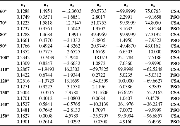
Unlike CSA, the PSO method is highly affected by parameter changes. However, the advantages of the algorithm are that it converges quickly and does not require too many parameters for the solution. In the PSO method, the swarm size (number of solutions) is 25, the lower and upper limits of the coefficients are −10 and +10, respectively, and the number of iterations, which is the stopping criterion of the algorithm, is 20000. There are studies indicating that swarm sizes between 10–30 give generally good results in PSO [Reference Engelbrecht53, Reference Oruc and Baklacioglu57]. In this context, the results were good at a value of 25, which was parallel to the literature. The most important point for the algorithm to give good results is to control the velocity. Although there are different methods for this, the constriction coefficients approach was used because it gives better results. The flowchart of the study is shown in Fig. 1. The comparison of the model results with the actual values for different inlet angles was shown in Figs. 2–11. Model coefficients values for different inlet angles are also shown in Table 1.

Figure 1.

Flowchart of study.

Figure 2.

Comparison of CSA/PSO noise models data with actual data for 60^° inlet angle.

Figure 3.

Comparison of CSA/PSO noise models data with actual data for 70^° inlet angle.

Figure 4.

Comparison of CSA/PSO noise models data with actual data for 80^° inlet angle.

Figure 5.

Comparison of CSA/PSO noise models data with actual data for 90^° inlet angle.

Figure 6.

Comparison of CSA/PSO noise models data with actual data for 100^° inlet angle.

Figs. 2–11 present the SPL values as a function of frequency at different inlet angles in the range of 60^°–150^°. As seen from the Figs. 2–11, the SPL value increases up to a certain level at low frequency values and then decreases as the frequency increases. In addition, the non-linear relation between SPL and frequency makes the optimisation process difficult with a single input. However, the Figs. 2–11 show that both algorithms give results that are compatible with the actual data despite this situation.

Figure 7.

Comparison of CSA/PSO noise models data with actual data for 110^° inlet angle.

Figure 8.

Comparison of CSA/PSO noise models data with actual data for 120^° inlet angle.

Figure 9.

Comparison of CSA/PSO noise models data with actual data for 130^° inlet angle.

Figure 10.

Comparison of CSA/PSO noise models data with actual data for 140^° inlet angle.

Figure 11.

Comparison of CSA/PSO noise models data with actual data for 150^° inlet angle.

When Figs. 2–11 for different microphone angles are examined, SPL values near maximum exhibit different characteristics. However, a common feature across all curves is that SPL values generally increase at low frequencies and decrease as frequency increases. This situation causes the modeling results to not be affected much for different microphone angles. Furthermore, the similarity of the curves for different microphone angles demonstrates the usability of a single model for all angles. As is the case in many areas of aviation, all available microphone angles were used because noise-related data is not generally shared by companies, manufacturers, authorities, etc. Using a wide range such as 60–150° in increments of 10 is important for measuring the applicability of the model. For different fighter aircraft, there is generally an increase in noise up to a certain value of the frequency, similar to the F22-A aircraft, and then a decrease in noise with increasing frequency. Therefore, since the curves show similar properties, it shows that the model obtained in the study can also be used in other aircraft [Reference Neilsen, Vaughn, Gee, Swift, Wall, Downing and James33, Reference Gee, Gabrielson, Atchley and Sparrow58]. In addition, the fact that the CSA method with the real data agrees better than the PSO shows its superior effectiveness in this field. The PSO model demonstrates a good agreement with the actual data at high inlet angles. However, at inlet angles of 60^°−70^°−80^°, the curve showed a slight deviation at frequencies above 6000. Nonetheless, the error assessment shows that the model is still applicable safely at these specified angles.

4.1 Error analysis

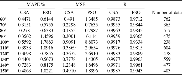
The accuracy of the algorithms has been examined using various error analysis methods. Model error values and the number of data sets used are shown in Table 2. In addition, the percentage error according to frequency for four different inlet angles (60–80–100–120) is shown in detail in Figs. 12–15, and histogram graphs showing the error values for other inlet angles are shown in Figs. 16–17.

Table 1.

PSO and CSA model coefficients

Table 2.

Model error values

One of the most important parameters affecting efficiency and reliability in modeling and optimisation studies is the large data set. Table 2 shows that the number of data points related to input angles ranges from 238 to 762, and a high data set is crucial for efficiency. Another important parameter for efficiency is validating model results. The validation method used in this study was to determine whether the model yielded low error values at other microphone angles with similar characteristics (tested for 10 different microphone angles). The error analysis results showed that a single model had a low error rate in predicting all microphone angles. This demonstrates the model’s suitability for all microphone angles for the F22-A aircraft. An examination of the error values reveals that the MAPE values for the CSA algorithm remain below 1% at all inlet angles. For the PSO algorithm, the maximum MAPE value is 1.7863%, indicating that the specified method can be used in this area. R parameter, which shows the agreement between the model data and the actual values, are also presented in Table 2. The closer this value is to 1, the better the fit. As observed in Table 2, the R values for CSA vary between 0.9873 and 0.9987, while for PSO this variation is between 0.9334 and 0.9963. The fact that R values are very close to 1 is another indicator of model’s high accuracy.

Figure 12.

Percentage error values for 60^° inlet angle.

Figure 13.

Percentage error values for 80^° inlet angle.

Figure 14.

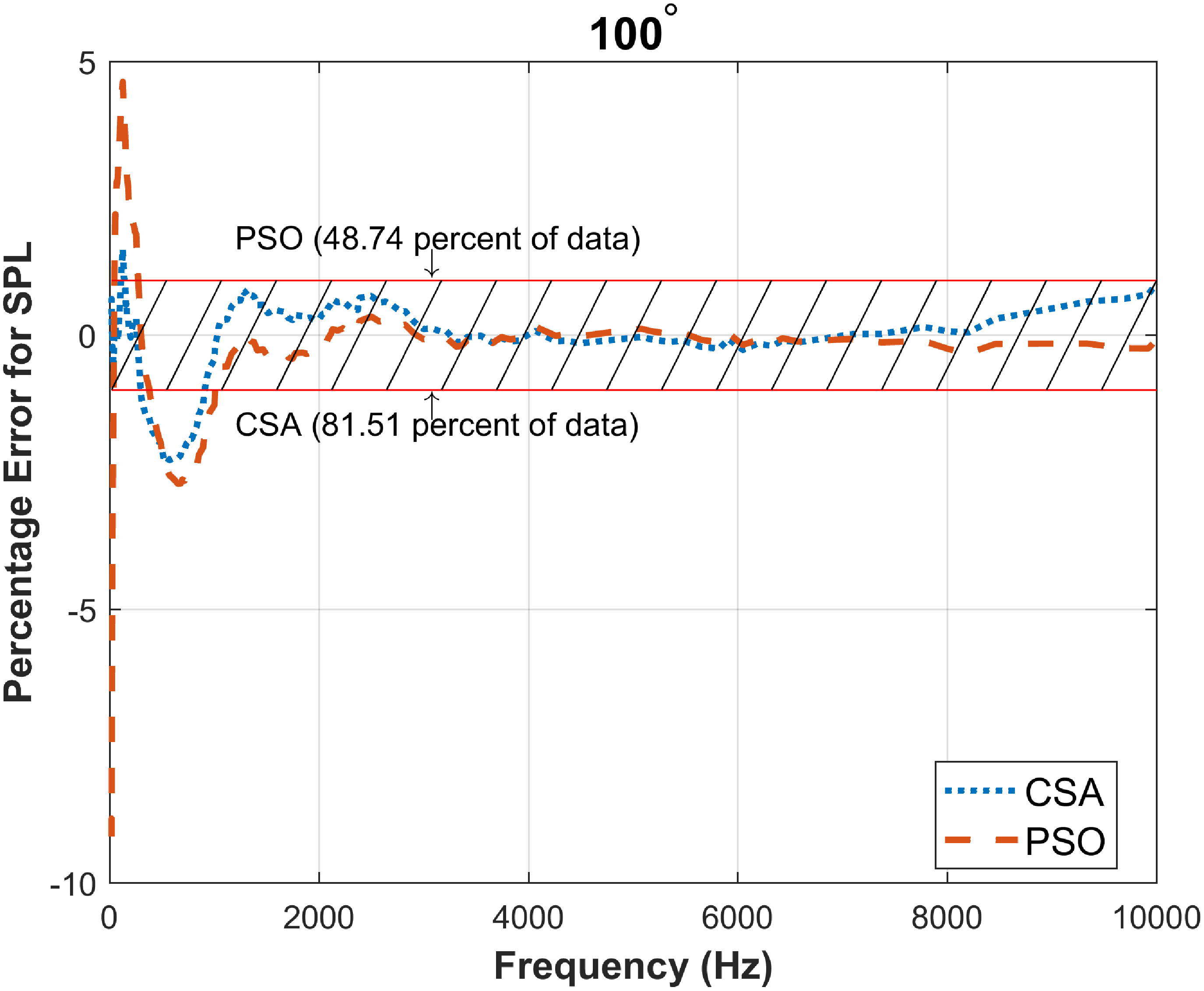
Percentage error values for 100^° inlet angle.

In the Figs. 12–15, the percentage error values between the values obtained with CSA and PSO and the actual values are shown according to frequency. When the specified figures are examined, it is seen that for the 60^° inlet angle, 90.94% of the data obtained with the CSA method is within 1% error and below, while for PSO, 82.15% is within the specified range. For other inlet angles, the number of data within the specified range for CSA is 81.51% and above. For CSA, the error rate of a very large data set being 1% or less shows the accuracy of the algorithm. For PSO, in Figs. 13–15, the data between −1 and 1 is 82.59% for 80^° inlet angle, 48.74% for 100^°, and 82.43% for 120^°. The main reason why half of the data for the 100^° input angle is in this range is that the error rate is a bit higher at low frequency. However, the fact that the data error rate outside of 1% is not very high, and that a large part of the data in the other two graphs (Fig. 13 and Fig. 15) is below 1%, proves that PSO is successful in this field.

Figure 15.

Percentage error values for 120^° inlet angle.

Figure 16.

The histogram of error for 70^°−90^°−110^° inlet angles.

Figure 17.

The histogram of error for 130^°−140^°−150^° inlet angles.

In Figs. 16 and 17, histogram graphs for different inlet angles are shown. The frequency on the y-axis was used to express the distribution of error values. When Figs 16 and 17 are examined, it is clearly seen that the error values are more concentrated in the region close to zero in both PSO and CSA methods at all input angles. This situation also approves the high accuracy of the models.