1 Introduction
In many astrophysical settings the magnetic field controls the overall dynamics of a plasma, while the dissipation of magnetic energy may power the high-energy emission. The relevant astrophysical settings include magnetars (strongly magnetized neutron stars possessing super-strong magnetic fields), pulsars and pulsar wind nebulae, jets of active galactic nuclei and gamma-ray bursters. All these objects are efficient emitters of X-rays and gamma rays, and in the past two decades they have been the subjects of intensive observational studies using a number of very successful high-energy satellites. These objects seem to share one important property – they include relativistic magnetized plasma, and often their plasma is magnetically dominated, i.e. the energy density of this plasma is dominated not by the rest mass energy of matter, but by the energy of the magnetic field. This is dramatically different from laboratory plasmas, the magnetospheres of planets and the interplanetary plasma.
Recently, these topics came to the front of astrophysical and plasma physical research. Particularly important was the discovery of flares from Crab Nebula (Abdo et al. Reference Abdo, Ackermann, Ajello, Allafort, Baldini, Ballet, Barbiellini and Bastieri2011; Tavani et al. Reference Tavani, Bulgarelli, Vittorini, Pellizzoni, Striani, Caraveo, Weisskopf and Tennant2011; Buehler et al. Reference Buehler, Scargle, Blandford, Baldini, Baring, Belfiore, Charles, Chiang, D’Ammando and Dermer2012), exhibiting unusually short durations, high luminosities and high photon energies. Exceptionally high peak energy of the flare spectral peak excludes stochastic shock acceleration as a mechanism of acceleration of flare-producing particles. An alternative possibility is that magnetic reconnection in highly magnetized plasma is responsible for the acceleration of the wind leptons (Lyutikov Reference Lyutikov2010; Clausen-Brown & Lyutikov Reference Clausen-Brown and Lyutikov2012; Cerutti et al. Reference Cerutti, Werner, Uzdensky and Begelman2013, Reference Cerutti, Werner, Uzdensky and Begelman2014). These events challenge our understanding of particle acceleration in Pulsar Wind Nebulae (PWNe), and, possibly in other high-energy astrophysical sources.
In conventional laboratory/space plasma, the merging of magnetic islands have been invoked as an important, and perhaps dominant, mechanism of particle acceleration (Oka et al. Reference Oka, Phan, Krucker, Fujimoto and Shinohara2010; Tanaka et al. Reference Tanaka, Yumura, Fujimoto, Shinohara, Badman and Grocott2010; Drake & Swisdak Reference Drake and Swisdak2012; Zank et al. Reference Zank, le Roux, Webb, Dosch and Khabarova2014). In this paper we investigate particle acceleration during magnetic island merger in relativistic highly magnetized plasmas. In order to describe the level of magnetization it is convenient to use the so-called magnetization parameter
 $$\begin{eqnarray}\unicode[STIX]{x1D70E}=2\frac{u_{B}}{u_{p}}=\frac{B^{2}}{4\unicode[STIX]{x03C0}\unicode[STIX]{x1D70C}c^{2}},\end{eqnarray}$$
where
 $u_{B}=B^{2}/8\unicode[STIX]{x03C0}$
is the magnetic energy density,
 $u_{p}=\unicode[STIX]{x1D70C}c^{2}$
is the rest mass energy density.
In Lyutikov et al. (Reference Lyutikov, Sironi, Komissarov and Porth2017, Paper I) we studied the plasma dynamics and particle acceleration during explosive collapse of a stressed X-point. In this paper we extends the work to include the large-scale dynamics. The key point of our approach is that the reconnection and particle acceleration is driven by macroscopic large-scale stresses of the magnetic field (and not, e.g. by effects on skin depth scales during the development of the tearing mode in collisionless plasma).
To include the effects of large-scale magnetic stresses we consider a number magnetic configurations: (i) two-dimensional (2-D) force-free magnetic flux tubes (ABC) configuration including the driven regimes § 3; (ii) colliding magnetic flux tubes carrying zero total current, § 4. The principal difference between these configurations is that in the case of 2-D force-free magnetic flux tubes each flux tube carries a non-zero total electric current – thus even far away flux tubes experience Lorentz attraction or repulsion.
2 Collapse of a system of magnetic islands
2.1 Two-dimensional magnetic ABC structures
In this section we consider large-scale dynamics that can lead to the X-point collapse described above. As an initial pre-flare state of plasma we consider a 2-D force-fee lattice of magnetic flux tubes
 $$\begin{eqnarray}\displaystyle \left.\begin{array}{@{}c@{}}B_{x}=-\text{sin}(2\unicode[STIX]{x03C0}\unicode[STIX]{x1D6FC}y)B_{0},\\ B_{y}=\sin (2\unicode[STIX]{x03C0}\unicode[STIX]{x1D6FC}x)B_{0},\\ B_{z}=\left(\cos (2\unicode[STIX]{x03C0}\unicode[STIX]{x1D6FC}x)+\cos (2\unicode[STIX]{x03C0}\unicode[STIX]{x1D6FC}y)\right)B_{0},\end{array}\right\} & & \displaystyle\end{eqnarray}$$
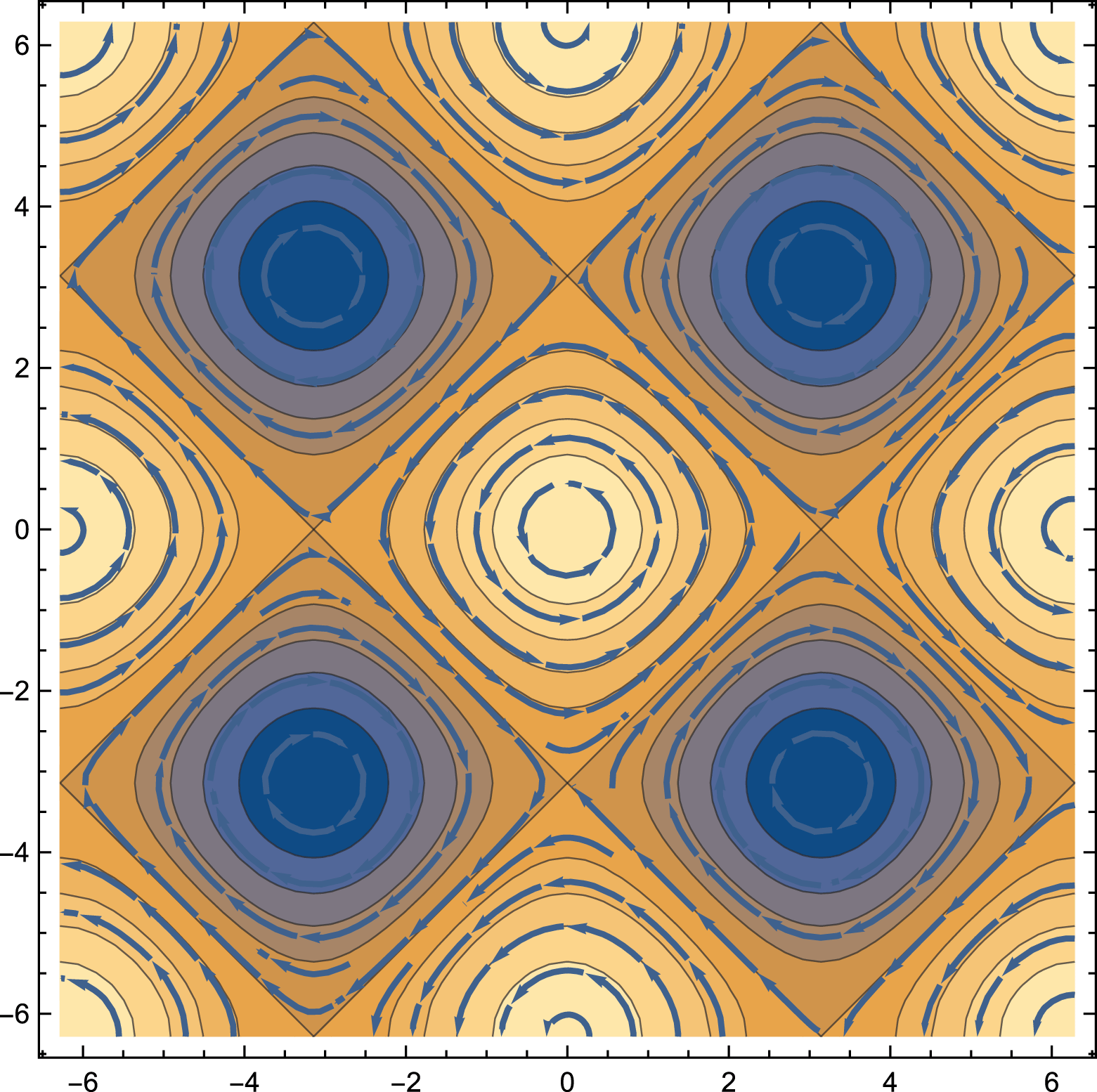
figure 1. This constitutes a lattice of force-free magnetic islands separated by
 $90^{\circ }$
X-points in equilibrium. Islands have alternating out-of-the-plane poloidal fields and alternating toroidal fields. Each magnetic flux tube carries a magnetic flux
 $\propto B_{0}/\unicode[STIX]{x1D6FC}^{2}$
, energy per unit length
 $\propto B_{0}^{2}/\unicode[STIX]{x1D6FC}^{2}$
, helicity per unit length
 $\propto B_{0}^{2}/(\unicode[STIX]{x1D6FC}^{3})$
and axial current
 $\propto B_{0}/(\unicode[STIX]{x1D6FC})$
. Helicity of both types of flux tube is of the same sign.
Previously, this configuration has been considered by Parker (Reference Parker1983) in the context of solar magnetic fields; he suggested that this force-free configuration is unstable. Later Longcope & Strauss (Reference Longcope and Strauss1994) considered the evolution of the instability. In the case of force-free plasma the instability has been recently considered by East, Zrake, Yuan & Blandford (Reference East, Zrake, Yuan and Blandford2015). The configuration (2.1) belongs to a family of ABC flows (Arnold-Beltrami-Childress, e.g. Roberts Reference Roberts1972). ABC magnetic structures are known to be stable to ideal perturbations (Arnold Reference Arnold1974; Molodensky Reference Molodensky1974; Moffatt Reference Moffatt1986) provided that all three corresponding coefficients are non-zero (though see East et al. Reference East, Zrake, Yuan and Blandford2015, for a claim to the contrary). Two-dimensional structures considered here do not satisfy this condition – in this case the islands can move with respect to each other, reducing their interaction energy, as we show below. The stable full 3-D ABC structures do not allow for such motion (see though East et al. (Reference East, Zrake, Yuan and Blandford2015) who claimed the instability of 3-D ABC configurations as well). Full 3-D ABC structures have all fields linked, while in the case of two dimensions the neighbouring cylinders are not linked together. The difference between stable 3-D and unstable 2-D ABC configurations illustrates a general principle that lower dimension magnetic structures are typically less stable.
We also point out that we start with configuration stable to internal kinks. For sufficiently high currents the non-constant-
 $\unicode[STIX]{x1D6FC}$
Lundquist-type configurations are known to show internal kink instabilities Voslamber & Callebaut (Reference Voslamber and Callebaut1962).
A 2-D force-free system of magnetic islands (magnetic ABC structures). Colour indicates out-of-the-plane magnetic field. Both types of islands have the same helicity. At the X-point the magnetic field and current are exactly zero.

2.2 The nature of the instability
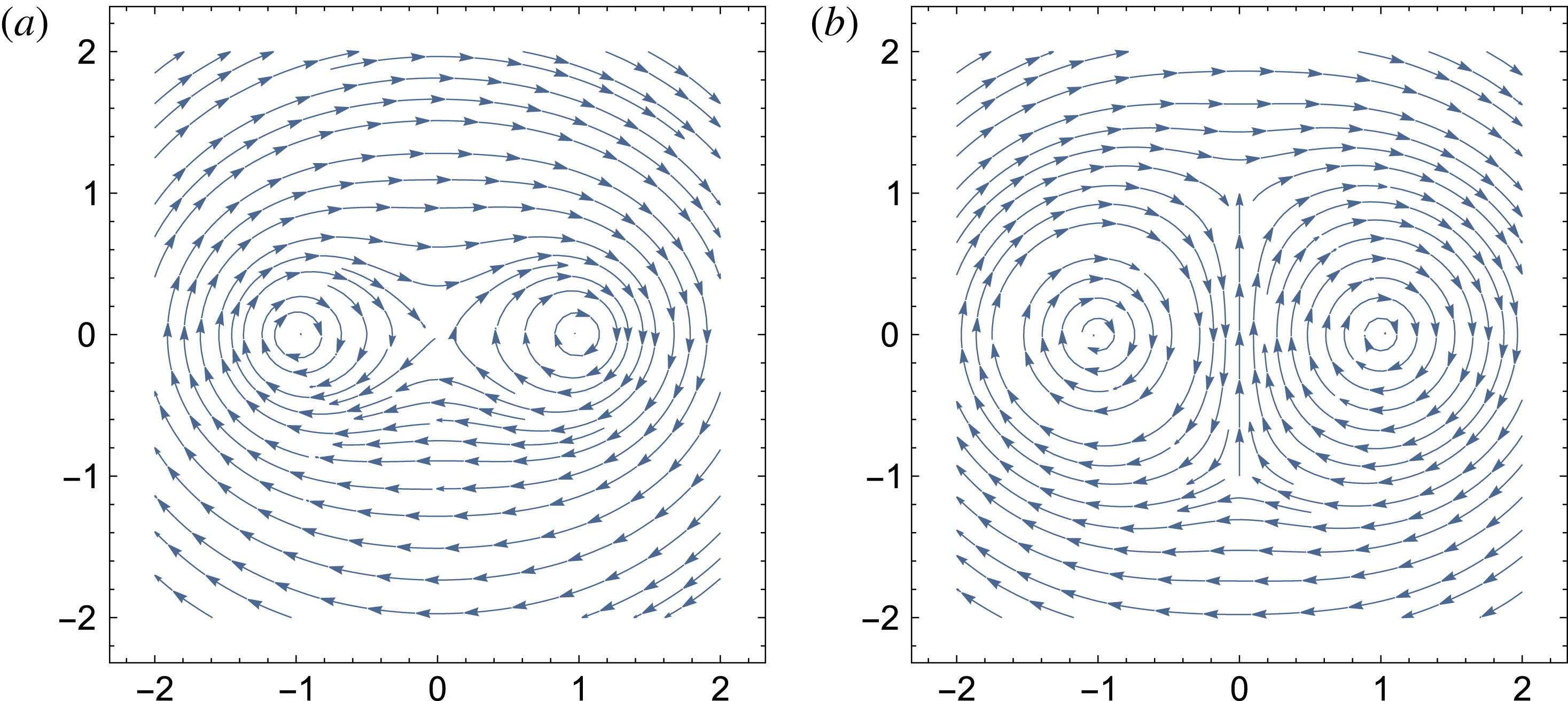
The instability of the 2-D ABC configuration is of the kind ‘parallel currents attract’. In the initial configuration the attraction of parallel currents is balanced by the repulsion of anti-parallel ones. Small amplitude fluctuations lead to fluctuating forces between the currents, that eventually lead to the disruption of the system. To identify the dominant instability mode let us consider a simplified model problem replacing each island by a solid tube carrying a given current. Such incompressible-type approximation is expected to be valid at early times, when the resulting motions are slow and the amount of the dissipated magnetic energy is small.
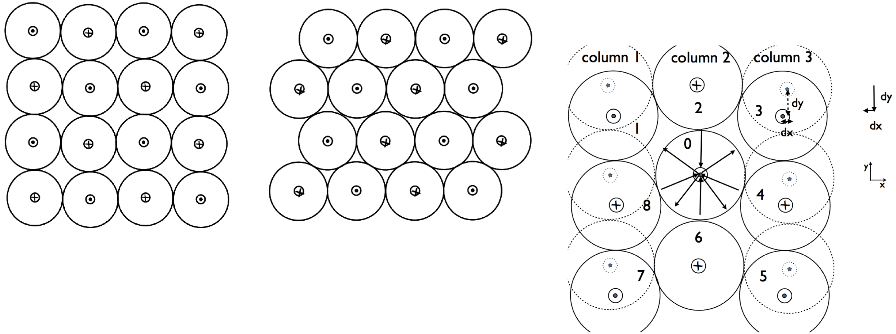
We identify two basic instability modes which we call the shear mode and the compression mode. Let us first consider a global shear mode, figure 2. Let us separate the 2-D ABC equilibrium into a set of columns, labelled 1–2–3, figure 2. In the initial state the flux tubes in the columns 1 and 3 (dashed lines) are horizontally aligned with those in column 2. Let us shift columns 1 and 3 by a value
 $-\text{d}y$
(or, equivalently, shift the column 2 by
 $+\text{d}y$
); corresponding horizontal displacement is
 $\text{d}x=\pm \text{d}y^{2}/2$
. Let us consider forces on the central island (labelled by
 $0$
in figure 2). The interaction of the central island with islands 4 and 8 produces a force in the positive
 $y$
direction
 $F_{y,4}+F_{y,8}\propto \text{d}y/2$
. The sum of forces
 $F_{y,1}+F_{y,3}+F_{y,5}+F_{y,7}\propto \text{d}y/2$
also produces a force in the positive vertical direction. From the symmetry of the problem it is clear that the sum of all the forces from all the islands produce a net force in the positive vertical direction – this amplifies the perturbations, leading to instability.
Qualitative picture of the development of shear-type (parallel) instability. The initial magnetic 2-D ABC structure (left panel) is unstable to long wavelength instability whereby each consecutive row is shifted by a half wavelength (right panel). A current sheet forms in between the islands with co-aligned currents leading to catastrophic merger. Right panel: the nature of the instability. Shifting alternating rows (or columns) of magnetic islands leads to a force imbalance that amplifies the perturbation. In the particular case, shifting first and third columns leads to a force along the positive direction on the islands in the second column, amplifying the perturbations.

We can also compare directly the corresponding interaction energies of the two states pictured in figure 2. Let us approximate each flux tube as a line current
 $I$
. Up to insignificant overall factor the interaction energy of two currents is
 $\propto I_{1}I_{2}\log r_{12}$
where
 $r_{12}$
is the distance between the two currents. Consider an arbitrary flux tube. It’s interaction with flux tubes located in the even row from a given one are the same in two cases. In the second case the interaction with flux tubes located in the odd rows is zero by symmetry, while in the initial state it is
 $$\begin{eqnarray}E_{odd}=\mathop{\sum }_{n=0}(-1)^{n}\ln \sqrt{n^{2}+(2m+1)^{2}},\end{eqnarray}$$
(here
 $2m+1,\,m=0,1,2,\ldots$
is the number of a row from a given island,
 $n=0,1,2,\ldots$
is the number of the islands in a row from a given island). This sum (2.2) is positive: the interaction energy with the
 $n=0$
island is always positive,
 $\propto \text{ln}((2m+1)r_{0})$
; the sum over
 $n$
th and
 $n+1$
islands is also positive,
 $\propto \text{ln}((n+1)^{2}+(2m+1)^{2})/(n^{2}+(2m+1)^{2})>0$
. Thus, the energy of the second state in figure 2 is lower – this is the driver of the instability.
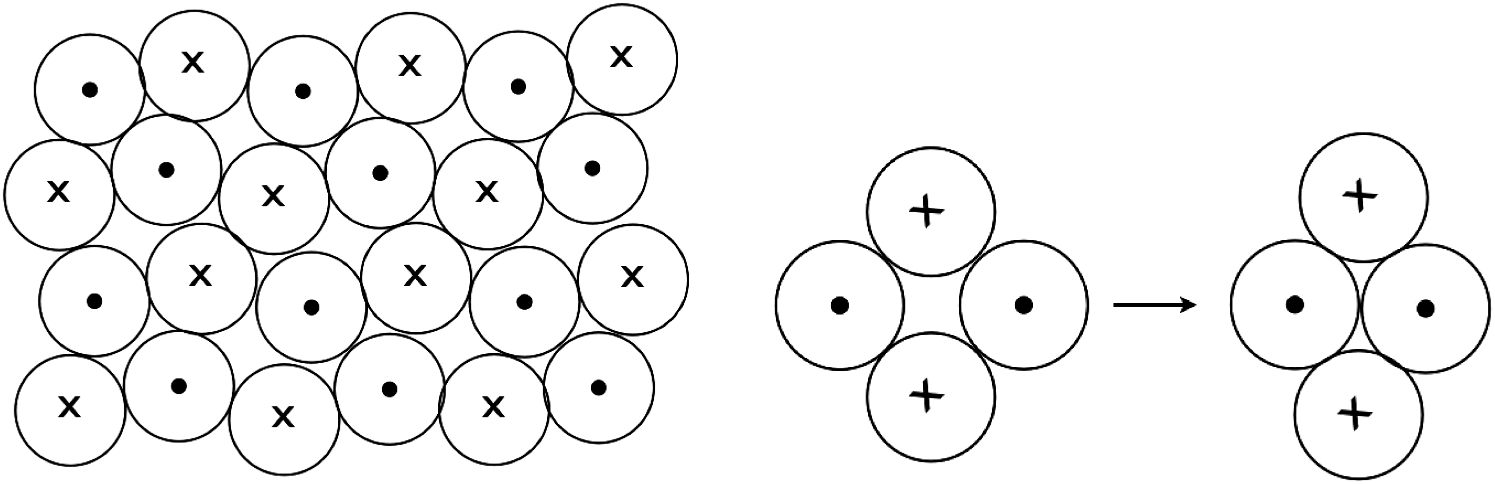
There is another instability mode that we identified, figure 3. Instead of coherent shift of the rows/columns it involve local rearrangement of two pairs of flux tubes, figure 3. This configuration has a lower energy than the initial state: the forces of interaction of each touching pair of currents with all other touching pairs of currents is zero by symmetry. Thus, what is important is the change in the energy for each two pairs of currents, left panel. It is negative and is
 $\propto -\text{ln}(2/\sqrt{3})$
.
Second (oblique) mode of instability.

This simple model problem demonstrates semi-qualitatively the exponentially growing instability of a system of magnetic islands. The instability initially is ideal and proceeds on the dynamical time scale of an island, so that perturbations grow to nonlinear stage in few dynamical time scales.
The above analytical considerations are clearly confirmed by numerical experiments as we discuss next.
2.3 Two-dimensional ABC instability: evolution in the force-free regime
2.3.1 Force-free simulations
Force-free simulations were carried out in a square domain of size
 $[-L,L]\times [-L,L]$
with 400 grid cells in each direction. Periodic boundary conditions were imposed on all boundaries. Four models with different magnetic Reynolds numbers
 $Re_{m}=4\unicode[STIX]{x03C0}\unicode[STIX]{x1D705}_{\Vert }L/c$
were investigated. figure 5 shows the evolution of the parameter
 $1-E^{2}/B^{2}$
, which is a Lorentz-invariant measure of the relative electric field strength, for the model with
 $Re_{m}=10^{3}$
. Until
 $t=7$
this parameter remains very close to zero throughout the whole domain, indicating the absence of current sheets and rapid motion in the bulk. Around
 $t=7$
, thin current sheets become visible in between magnetic islands (see figure 5
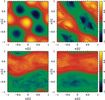
a). After this time the evolution proceeds rapidly – small islands merge to form larger ones until only two islands remain as one can also see in figure 6, which shows the evolution of
 $B_{z}$
. Models with higher
 $Re_{m}$
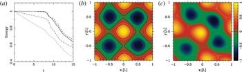
show very similar evolution, with almost the same time for the onset of mergers and the same rate of magnetic dissipation after that. Figure 7 shows the evolution of the total electromagnetic energy in the box. One can see that for
 $t<7$
, the energy significantly decreases in models with
 $Re_{m}=10^{3}$
and
 $Re_{m}=2\times 10^{3}$
due to the ohmic dissipation, whereas it remains more or less unchanged in the models with
 $Re_{m}>5\times 10^{3}$
. The first ‘knee’ on each curve corresponds to the onset of the first wave of merges. At
 $t>7$
the magnetic dissipation rate no longer depends on
 $Re_{m}$
. The characteristic time scale of the process is very short – only a few light crossings of the box.
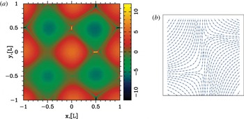
(a) Initial stage of the development of instability in force-free simulations. The colour image shows the distribution of the current density
 $j_{z}$
at
 $t=7.4$
in the model with
 $Re_{m}=10^{3}$
. The newly formed current sheets are clearly visible. (b) The development of the current sheet due to a shift of magnetic islands in the theoretical model (in the initial configuration 2-D ABC magnetic structure the two nearby rows of magnetic islands are shifted by some amount; this produces highly stressed configuration that would lead to X-point collapse).

Overall, the numerical results agree with our theoretical analysis (§§ 2–5). The fact that the onset of mergers does not depend on
 $Re_{m}$
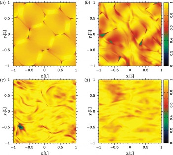
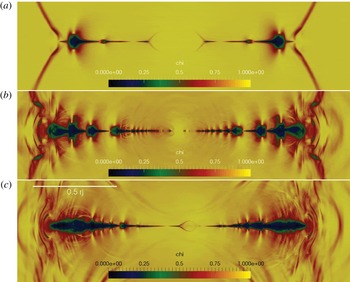
supports the conclusion that the evolution starts as an ideal instability, driven by the large-scale magnetic stresses. This instability leads to the relative motion of flux tubes and development of stressed X-points, with highly unbalanced magnetic tension. They collapse and form current sheets (see figure 4).
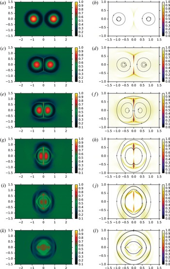
X-point collapse and island merging for a set of unstressed magnetic islands in force-free simulations. We plot
 $1-E^{2}/B^{2}$
at times
 $t=8.0,10.0,15.0$
and 20. Compare with the results of PIC simulations, figure 12.

Until
 $t\leqslant 7$
the instability develops in the linear regime and the initial periodic structure is still well preserved. At the nonlinear stage, at
 $t\geqslant 7$
, two new important effects come into play. Firstly, the magnetic reconnection leads to the emergence of closed magnetic field lines around two or more magnetic islands of similar polarity (see figure 7). Once formed, the common magnetic shroud pushes the islands towards the reconnection region in between via magnetic tension. Thus, this regime can be called a forced reconnection. As the reconnection proceeds, more common magnetic field lines develop, increasing the driving force. Secondly, the current of the current sheet separating the merging islands becomes sufficiently large to slow down the merger via providing a repulsive force (§ 5). Hence, the reconnection rate is determined both by the resistivity of the current sheet and the overall magnetic tension of common field lines.
We have studied the same problem using Particle-on-cell (PIC) simulations of highly magnetized plasma and their results are strikingly similar (compare figures 4–6 with figures 12 and 13). Not only do they exhibit the same phases of evolution, but also very similar time scales. This shows that the details of the microphysics are not important and the key role is played by the large-scale magnetic stresses.
X-point collapse and island merging for a set of unstressed magnetic islands in force-free simulations. We plot
 $B_{z}/2B_{0}$
at times
 $t=8.0,10.0,15.0$
and 20.

(a) Evolution of the total electromagnetic energy in the computational domain for the force-free models with
 $Re_{m}=10^{3}$
(dotted),
 $2\times 10^{3}$
(dash-dotted),
 $5\times 10^{3}$
(dashed) and
 $2\times 10^{4}$
(solid). In all models, the merger phase starts around
 $t=8$
, which corresponds to the first ‘knee’ of these curves. Compare the temporal evolution of the electromagnetic in force-free simulations with those in PICs, figure 9. (b,c) Solutions at
 $t=7.2$
(left) and
 $t=8$
(right) for the model with
 $Re_{m}=10^{3}$
. The colour coded image shows
 $B_{z}/2B_{0}$
. The contours are the magnetic field lines. One can see that some lines have become common for several islands.

2.4 Two-dimensional ABC instability: PIC simulations
We study the evolution of 2-D ABC structures with PIC simulations, employing the electromagnetic PIC code TRISTAN-MP (Buneman Reference Buneman1993; Spitkovsky Reference Spitkovsky, Bulik, Rudak and Madejski2005) (independently, a closely related study has been recently published by Nalewajko et al. Reference Nalewajko, Zrake, Yuan, East and Blandford2016).
To the best of our knowledge, our investigation is the first to address with PIC simulations the dynamics and particle acceleration of high-magnetization ABC structures.
Our computational domain is a square in the
 $x{-}y$
plane with periodic boundary conditions in both directions. The simulation box is initialized with a uniform density of electron–positron plasma at rest, a vanishing electric field and with the magnetic field appropriate for the 2-D ABC configuration, as described in (2.1). In addition to the unstressed geometry in (2.1), we also investigate the case of 2-D magnetic structures with an initial stress, or with an initial velocity shear, as we specify below.
For our fiducial runs, the spatial resolution is such that the plasma skin depth
 $\,c/\unicode[STIX]{x1D714}_{p}$
is resolved with 2.5 cells, but we have verified that our results are the same up to a resolution of
 $\,c/\unicode[STIX]{x1D714}_{p}=10$
cells. Since we investigate the case of both cold and hot background plasmas, our definition of the skin depth is
 $\,c/\unicode[STIX]{x1D714}_{p}=\sqrt{mc^{2}[1+(\hat{\unicode[STIX]{x1D6FE}}-1)^{-1}kT/mc^{2}]/4\unicode[STIX]{x03C0}ne^{2}}$
, where
 $\hat{\unicode[STIX]{x1D6FE}}$
is the adiabatic index. Each cell is initialized with two positrons and two electrons, but we have checked that our results are the same when using up to 16 particles per cell. In order to reduce noise in the simulation, we filter the electric current deposited onto the grid by the particles, mimicking the effect of a larger number of particles per cell (Spitkovsky Reference Spitkovsky, Bulik, Rudak and Madejski2005; Belyaev Reference Belyaev2015).
Our unit of length is the diameter
 $L$
of the ABC structures, and time is measured in units of
 $L/c$
. Typically, our domain is a square of side
 $2L$
, but we have investigated also rectangular domains with size
 $2L\times L$
, and large square domains with dimensions
 $4L\times 4L$
. In addition to the shape of the domain, we also vary the flow parameters, such as the temperature of the background plasma (
 $kT/mc^{2}=10^{-4}$
,
 $10$
and
 $10^{2}$
) and the flow magnetization. The general definition of the magnetization is
 $\unicode[STIX]{x1D70E}=B^{2}/4\unicode[STIX]{x03C0}w$
, where
 $w=nmc^{2}+\hat{\unicode[STIX]{x1D6FE}}p/(\hat{\unicode[STIX]{x1D6FE}}-1)$
; here,
 $w$
is the enthalpy,
 $p$
is the pressure and
 $\hat{\unicode[STIX]{x1D6FE}}$
is the adiabatic index. In the following, we identify our runs via the mean value
 $\unicode[STIX]{x1D70E}_{in}$
of the magnetization measured with the in-plane fields (so, excluding the
 $B_{z}$
field). As we argue below, it is the dissipation of the in-plane fields that primarily drives efficient heating and particle acceleration. The mean in-plane field corresponding to
 $\unicode[STIX]{x1D70E}_{in}$
shall be called
 $B_{0,in}$
, and it will be our unit of measure of the electromagnetic fields. For the 2-D ABC geometry,
 $B_{0,in}$
is equal to the field
 $B_{0}$
in (2.1). We will explore a wide range of magnetizations, from
 $\unicode[STIX]{x1D70E}_{in}=3$
up to
 $\unicode[STIX]{x1D70E}_{in}=680$
. The mean magnetization of the system, including all the magnetic field components, is
 $2\unicode[STIX]{x1D70E}_{in}$
.
It will be convenient to compare the diameter
 $L$
of ABC structures to the characteristic Larmor radius
 $r_{L,\text{hot}}=\sqrt{\unicode[STIX]{x1D70E}_{in}}\,c/\unicode[STIX]{x1D714}_{p}$
of the high-energy particles heated/accelerated by reconnection (rather than to the skin depth
 $\,c/\unicode[STIX]{x1D714}_{p}$
). We will explore a wide range of
 $L/r_{L,\text{hot}}$
, from
 $L/r_{L,\text{hot}}=31$
up to
 $502$
. We will demonstrate that the two most fundamental parameters that characterize a system of 2-D ABC structures are the magnetization
 $\unicode[STIX]{x1D70E}_{in}$
and the ratio
 $L/r_{L,\text{hot}}$
.
In the following, we will quantify the upper cutoff of the particle energy spectrum as
 $\unicode[STIX]{x1D6FE}_{\text{max}}$
, defined as
 $$\begin{eqnarray}\unicode[STIX]{x1D6FE}_{\text{max}}=\frac{\displaystyle \int \unicode[STIX]{x1D6FE}^{n_{\text{cut}}}\,\text{d}N/\text{d}\unicode[STIX]{x1D6FE}\,\text{d}\unicode[STIX]{x1D6FE}}{\displaystyle \int \unicode[STIX]{x1D6FE}^{n_{\text{cut}}-1}\,\text{d}N/\text{d}\unicode[STIX]{x1D6FE}\,\text{d}\unicode[STIX]{x1D6FE}}\end{eqnarray}$$
where
 $n_{\text{cut}}$
is empirically chosen to be
 $n_{\text{cut}}=6$
. If the particle energy spectrum takes the form
 $\text{d}N/\text{d}\unicode[STIX]{x1D6FE}\propto \unicode[STIX]{x1D6FE}^{-s}\exp (-\unicode[STIX]{x1D6FE}/\unicode[STIX]{x1D6FE}_{\text{cut}})$
with power-law slope
 $s$
and exponential cutoff at
 $\unicode[STIX]{x1D6FE}_{\text{cut}}$
, then our definition yields
 $\unicode[STIX]{x1D6FE}_{\text{max}}\sim (n_{\text{cut}}-s)\,\unicode[STIX]{x1D6FE}_{\text{cut}}$
.
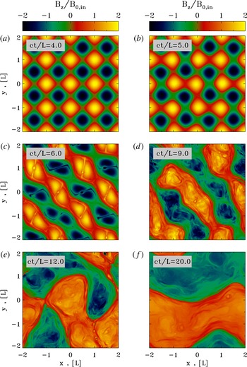
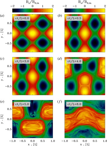
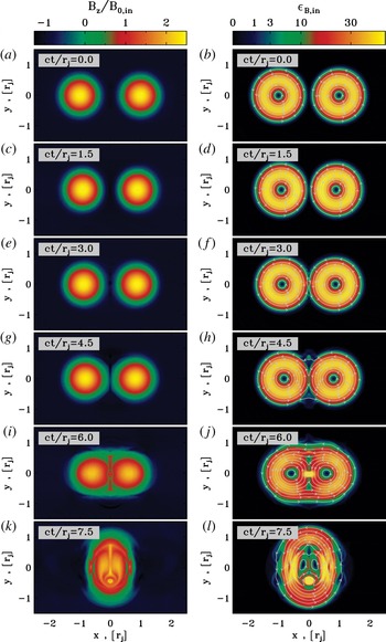
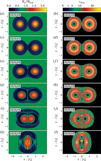
Temporal evolution of the instability of a typical 2-D ABC structure (time is indicated in the grey box of a–f). The plot presents the 2-D pattern of the out-of-plane field
 $B_{z}$
(in units of
 $B_{0,in}$
) from a PIC simulation with
 $kT/mc^{2}=10^{2}$
,
 $\unicode[STIX]{x1D70E}_{in}=42$
and
 $L=126\,r_{L,\text{hot}}$
, performed within a large square domain of size
 $4L\times 4L$
. The system stays unperturbed until
 $ct/L\simeq 4$
, then it goes unstable via the oblique mode presented in figure 2. The instability leads to the formation of current sheets of length
 ${\sim}L$
(at
 $ct/L=6$
), and to the merger of islands with
 $B_{z}$
fields of the same polarity. At the final time, the box is divided into two regions with
 $B_{z}$
fields of opposite polarity. This should be compared with the force-free results in figure 6.

2.4.1 The instability of 2-D ABC structures
Figure 8 illustrates the instability of a typical 2-D ABC structure. The plot presents the 2-D pattern of the out-of-plane field
 $B_{z}$
(in units of
 $B_{0,in}$
) from a PIC simulation with
 $kT/mc^{2}=10^{2}$
,
 $\unicode[STIX]{x1D70E}_{in}=42$
and
 $L=126\,r_{L,\text{hot}}$
, performed within a large square domain of size
 $4L\times 4L$
. Time is measured in units of
 $L/c$
and indicated in the grey boxes within each panel. The system does not show any evidence of evolution until
 $ct/L\sim 4$
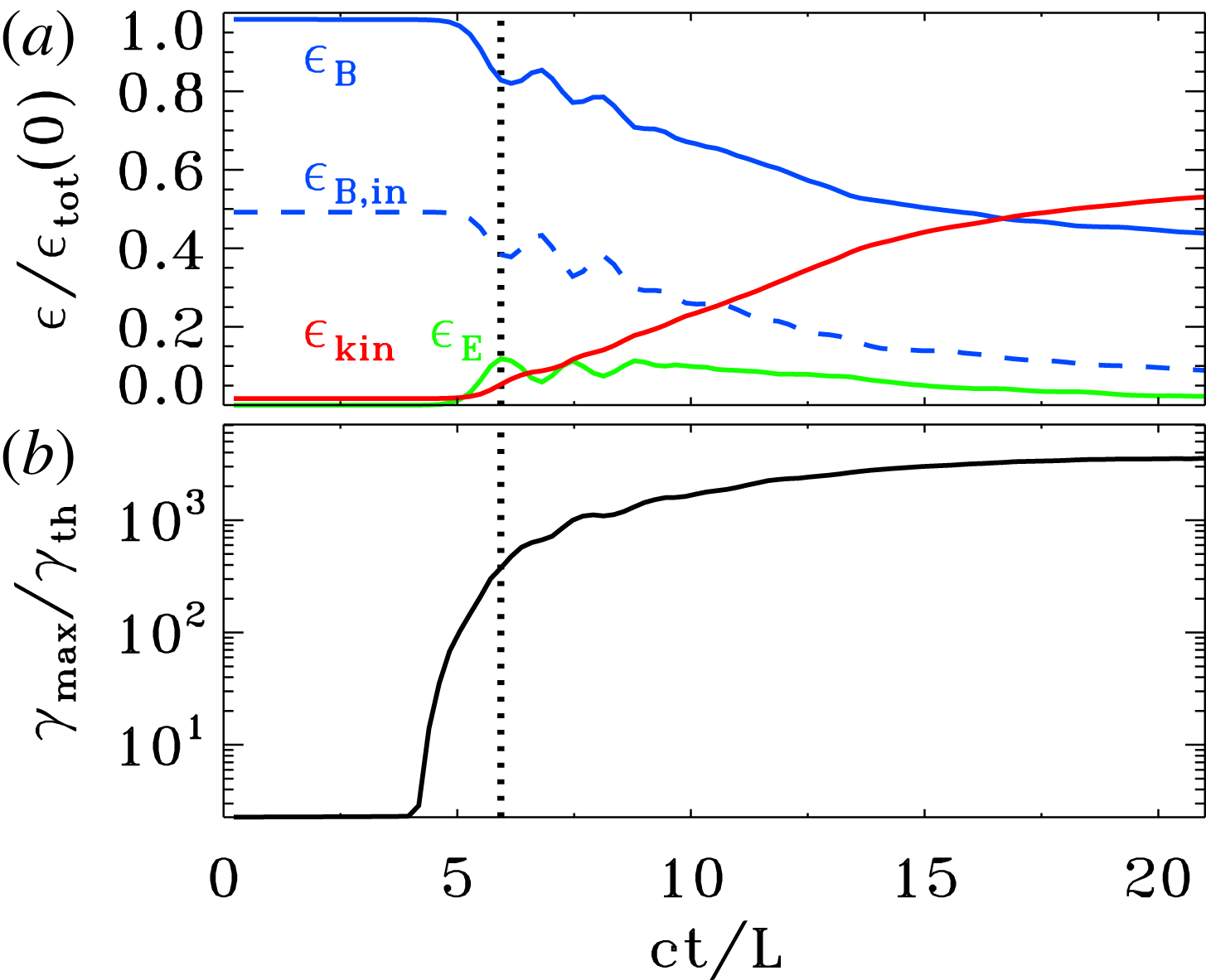
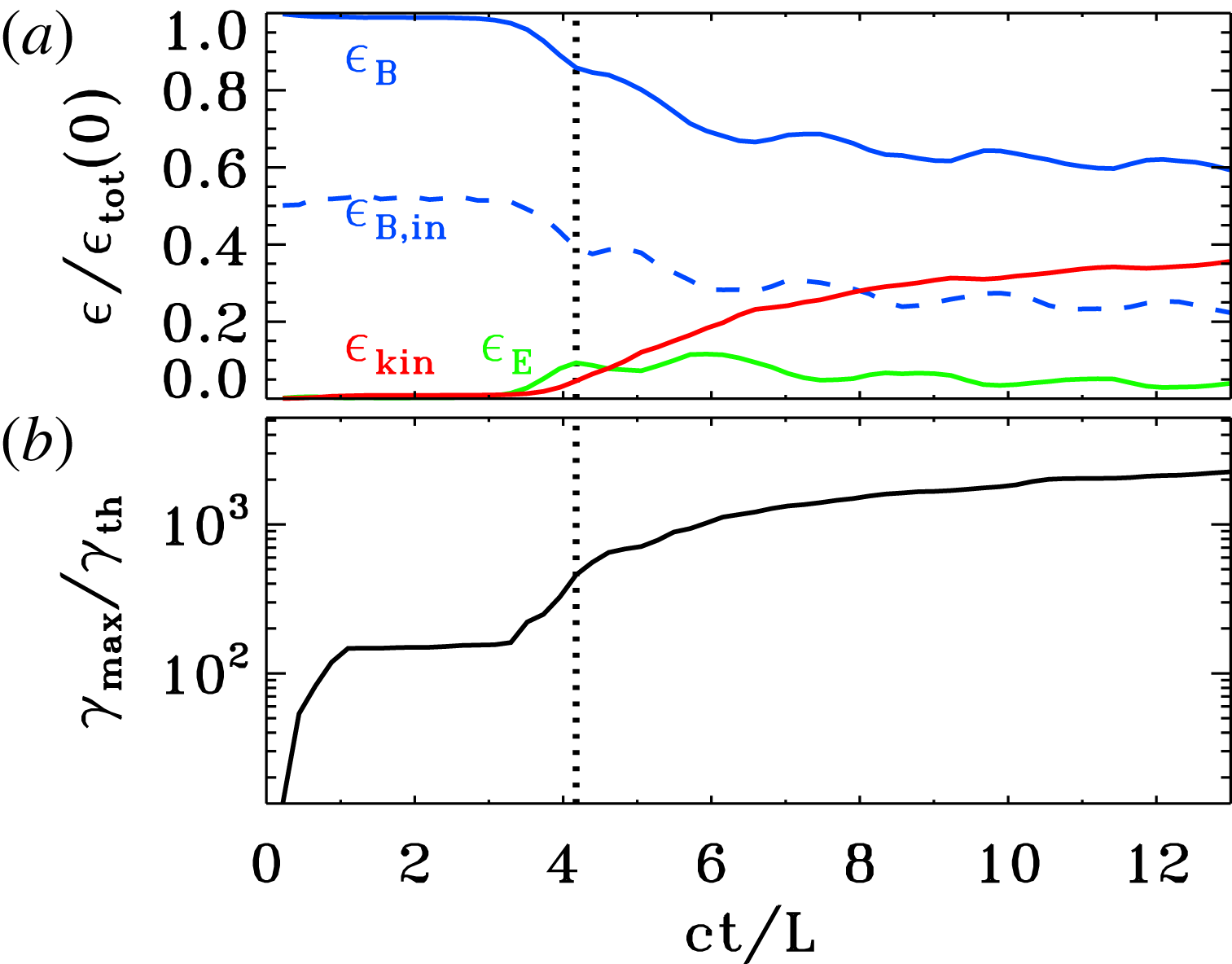
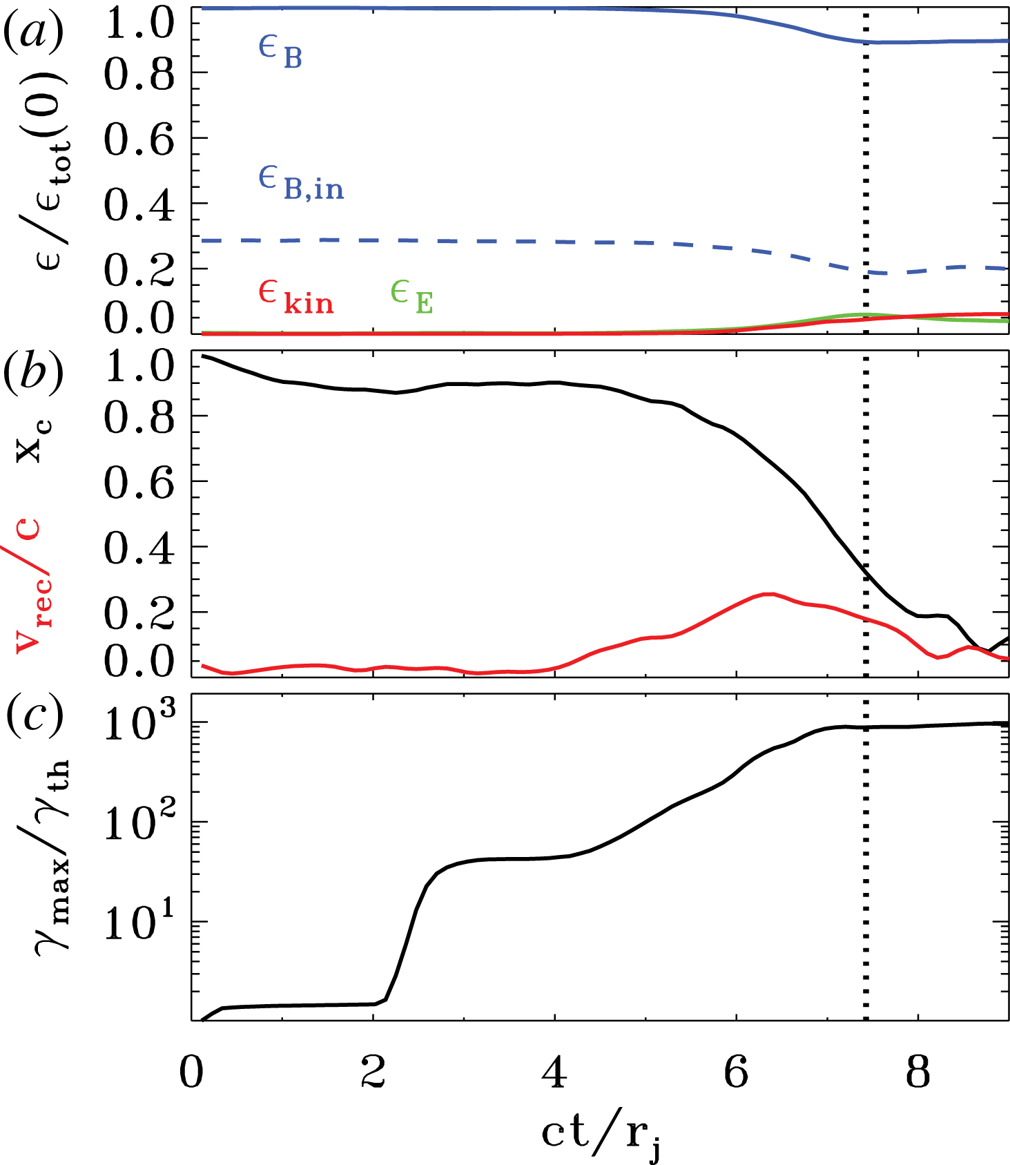
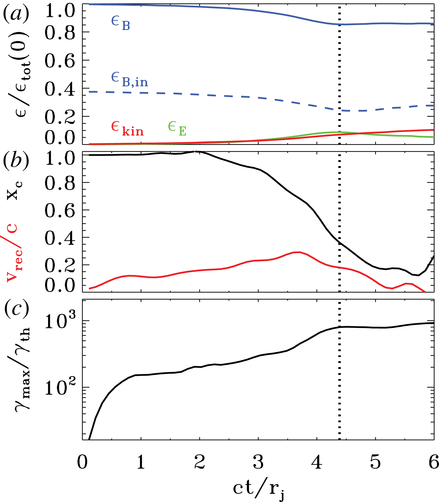
. This is also confirmed by the temporal tracks shown in figure 9, where (a) presents the energy partition among different components. Until
 $ct/L\sim 4$
, all the energy is still in the magnetic field (solid blue line), and the state of the system is identical to the initial set-up.
Quite abruptly, at
 $ct/L\sim 5$
(figure 8
b), the system becomes unstable. The pattern of magnetic islands shifts along the oblique direction, in analogy to the mode illustrated in figure 2. In agreement with the fluid simulations presented by East et al. (Reference East, Zrake, Yuan and Blandford2015), our PIC results confirm that this is an ideal instability. The onset time is comparable to what is observed in force-free simulations (see figure 7) and it does not appreciably depend on numerical parameters (so, on the level of numerical noise). In particular, we find no evidence for an earlier onset time when degrading our numerical resolution (spatial resolution or number of particles per cell). As we show below, the onset time at
 $ct/L\sim 5$
is also remarkably independent of physical parameters, with only a moderate trend for later onset times at larger values of
 $L/r_{L,\text{hot}}$
. We have also investigated the dependence of the onset time on the number of ABC islands in the computational domain (or equivalently, on the box size in units of
 $L$
). We find that square domains with
 $2L\times 2L$
or
 $4L\times 4L$
yield similar onset times, whereas the instability is systematically delayed (by a few
 $L/c$
) in rectangular boxes with
 $2L\times L$
, probably because this reduces the number of modes that can go unstable (in fact, we have verified that ABC structures in a periodic square box of size
 $L\times L$
are stable). We conclude that the abrupt evolution observed at times
 $ct/L\geqslant 5$
is physically motivated – this the stage where the instabilities reaches a nonlinear stage.
Following the instability onset, the evolution of the system proceeds on the dynamical time. Within a few
 $L/c$
, as they drift along the oblique direction, neighbouring islands with the same
 $B_{z}$
polarity come into contact (figure 8(c) at
 $ct/L=6$
), the X-points in between each pair of islands collapse under the effect of large-scale stresses (see Paper I), and thin current sheets are formed. For the parameters of figure 8, the resulting current sheets are so long that they are unstable to the secondary tearing mode (Uzdensky, Loureiro & Schekochihin Reference Uzdensky, Loureiro and Schekochihin2010), and secondary plasmoids are formed (e.g. see the plasmoid at
 $(x,y)=(-1.5L,L)$
at
 $ct/L=6$
). Below, we demonstrate that the formation of secondary plasmoids is primarily controlled by the ratio
 $L/r_{L,\text{hot}}$
. At the X-points, the magnetic energy is converted into particle energy by a reconnection electric field of order
 ${\sim}0.3B_{in}$
, where
 $B_{in}$
is the in-plane field (so, the reconnection rate is
 $v_{\text{rec}}/c\sim 0.3$
).Footnote
1
As shown in figure 9(a), it is primarily the in-plane field that gets dissipated (compare the dashed and solid blue lines), driving an increase in the electric energy (green) and in the particle kinetic energy (red).Footnote
2
In this phase of evolution, the fraction of initial energy released to the particles is still small (
 $\unicode[STIX]{x1D716}_{\text{kin}}/\unicode[STIX]{x1D716}_{\text{tot}}(0)\sim 0.1$
), but the particles advected into the X-points experience a dramatic episode of acceleration. As shown in figure 9(b), the cutoff Lorentz factor
 $\unicode[STIX]{x1D6FE}_{\text{max}}$
of the particle spectrum presents a dramatic evolution, increasing from the thermal value
 $\unicode[STIX]{x1D6FE}_{th}\simeq 3kT/mc^{2}$
(here,
 $kT/mc^{2}=10^{2}$
) by a factor of
 $10^{3}$
within a couple of dynamical times. It is this phase of extremely fast particle acceleration that we associate with the generation of the Crab flares.
Temporal evolution of various quantities, from a 2-D PIC simulation of ABC instability with
 $kT/mc^{2}=10^{2}$
,
 $\unicode[STIX]{x1D70E}_{in}=42$
and
 $L=126\,r_{L,\text{hot}}$
, performed within a large square domain of size
 $4L\times 4L$
(the same run as in figure 8). (a) Fraction of energy in magnetic fields (solid blue), in-plane magnetic fields (dashed blue, with
 $\unicode[STIX]{x1D716}_{B,in}=\unicode[STIX]{x1D716}_{B}/2$
in the initial configuration), electric fields (green) and particles (red; excluding the rest mass energy), in units of the total initial energy. Compare the temporal evolution of the electromagnetic in PIC simulations with those that are force free, figure 7. (b) Evolution of the maximum Lorentz factor
 $\unicode[STIX]{x1D6FE}_{\text{max}}$
, as defined in (2.3), relative to the thermal Lorentz factor
 $\unicode[STIX]{x1D6FE}_{th}\simeq 1+(\hat{\unicode[STIX]{x1D6FE}}-1)^{-1}kT/mc^{2}$
, which for our case is
 $\unicode[STIX]{x1D6FE}_{th}\simeq 300$
. The development of the instability at
 $ct/L\simeq 5$
is accompanied by little field dissipation (
 $\unicode[STIX]{x1D716}_{\text{kin}}/\unicode[STIX]{x1D716}_{\text{tot}}(0)\sim 0.1$
) but dramatic particle acceleration. (a,b) Vertical dotted black line indicates the time when the electric energy peaks, which happens shortly before the end of the most violent phase of instability.

Over one dynamical time, the current sheets in between neighbouring islands stretch to their maximum length of
 ${\sim}L$
. This corresponds to the time when the electric energy peaks, which is indicated by the dotted black line in figure 9, and it shortly precedes the end of the most violent phase of instability. The peak time of the electric energy will be a useful reference point when comparing runs with different physical parameters. The first island merger event ends at
 $ct/L\sim 7$
with the coalescence of island cores. At later times, the system of magnetic islands will undergo additional merger episodes (i.e. at
 $ct/L\sim 9$
and 12), with the formation of current sheets and secondary plasmoids (see e.g. at
 $(x,y)=(L,-1.5L)$
in figure 8
e), but the upper cutoff of the particle spectrum will not change by more than a factor of three (see figure 9
b at
 $ct/L\gtrsim 6$
). As a consequence, the spectral cutoff at the final time is not expected to be significantly dependent on the number of lengths
 $L$
in the computational domain, as we have indeed verified. Rather than dramatic acceleration of a small number of ‘lucky’ particles, the late phases result in substantial heating of the bulk of the particles, as illustrated by the red line in figure 9(a). As a consequence of particle heating, the effective magnetization of the plasma is only
 $\unicode[STIX]{x1D70E}_{in}\sim 1$
after the initial merger episode (compare the dashed blue and solid red lines at
 $ct/L\sim 9$
and 12 in figure 9
a), which explains why additional island mergers do not lead to dramatic particle acceleration. The rate of dissipation of magnetic energy into particle energy at late times is approximately consistent with the results of force-free simulations (see figure 7). At late times, the system saturates when only two regions are left in the box, having
 $B_{z}$
fields of opposite polarity (figure 8
f). In the final state, most of the in-plane magnetic energy has been transferred to the particles (compare the red and dashed blue lines in figure 9
a).
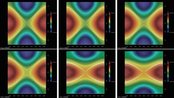
In figure 13 we compare the development of the two modes of instability, the parallel and the oblique one.
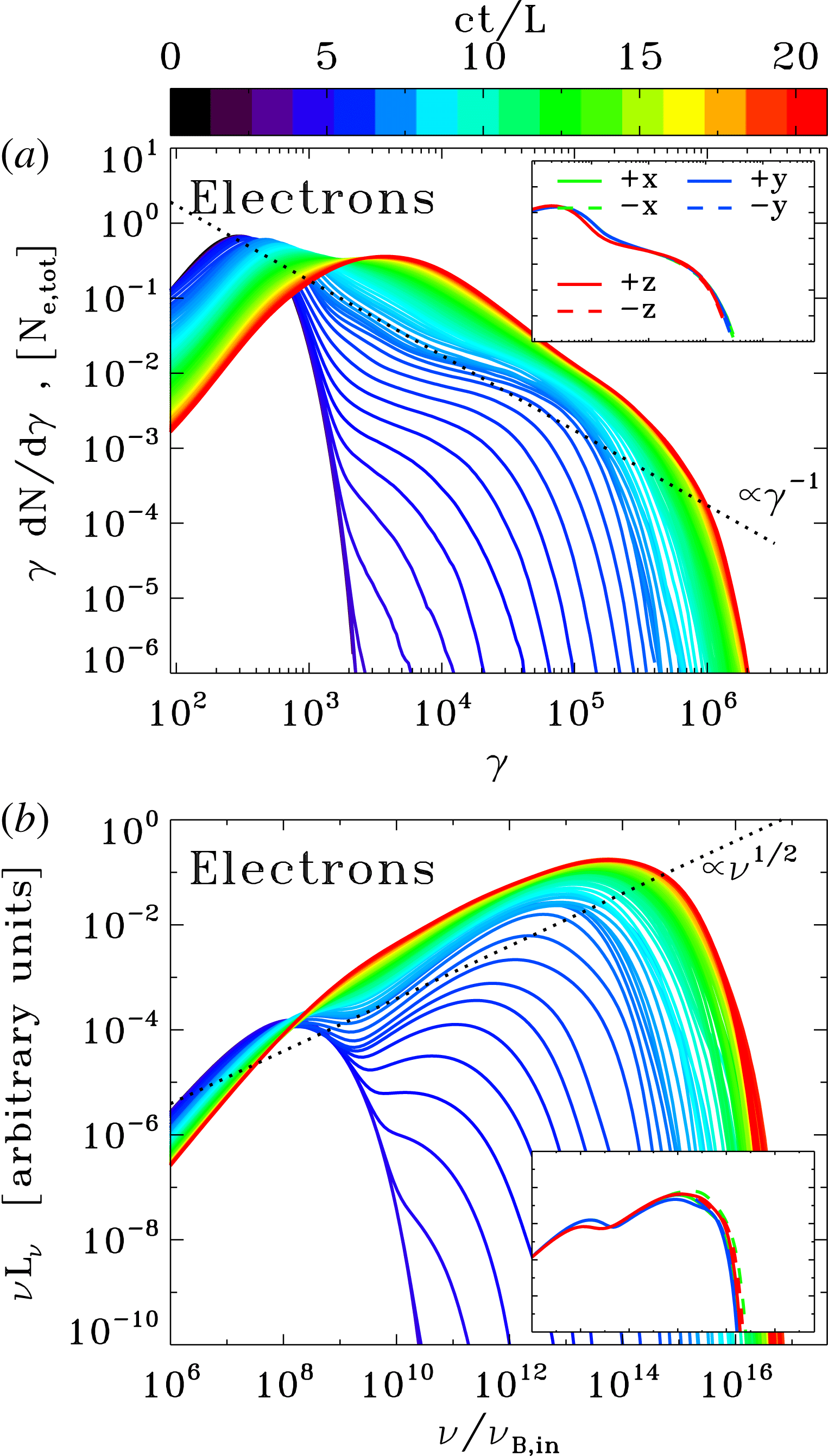
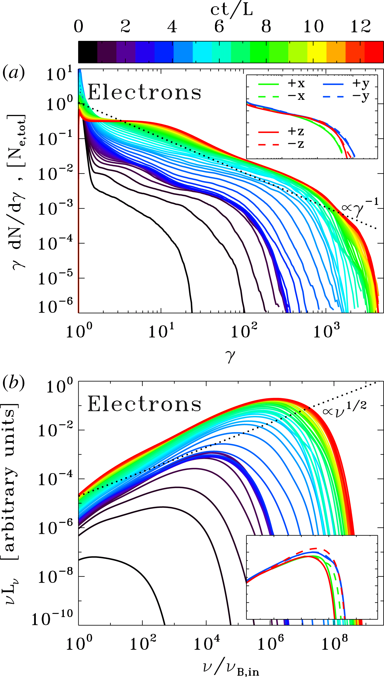
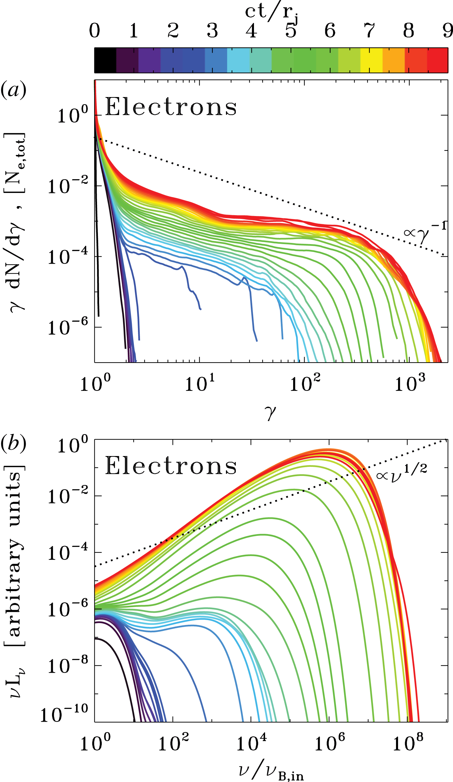
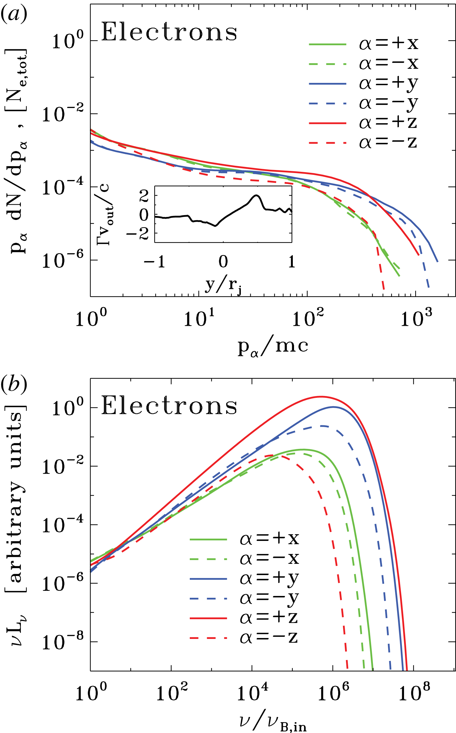
Particle spectrum and synchrotron spectrum from a 2-D PIC simulation of ABC instability with
 $kT/mc^{2}=10^{2}$
,
 $\unicode[STIX]{x1D70E}_{in}=42$
and
 $L=126\,r_{L,\text{hot}}$
, performed within a large square domain of size
 $4L\times 4L$
(the same run as in figures 8 and 9). Time is measured in units of
 $L/c$
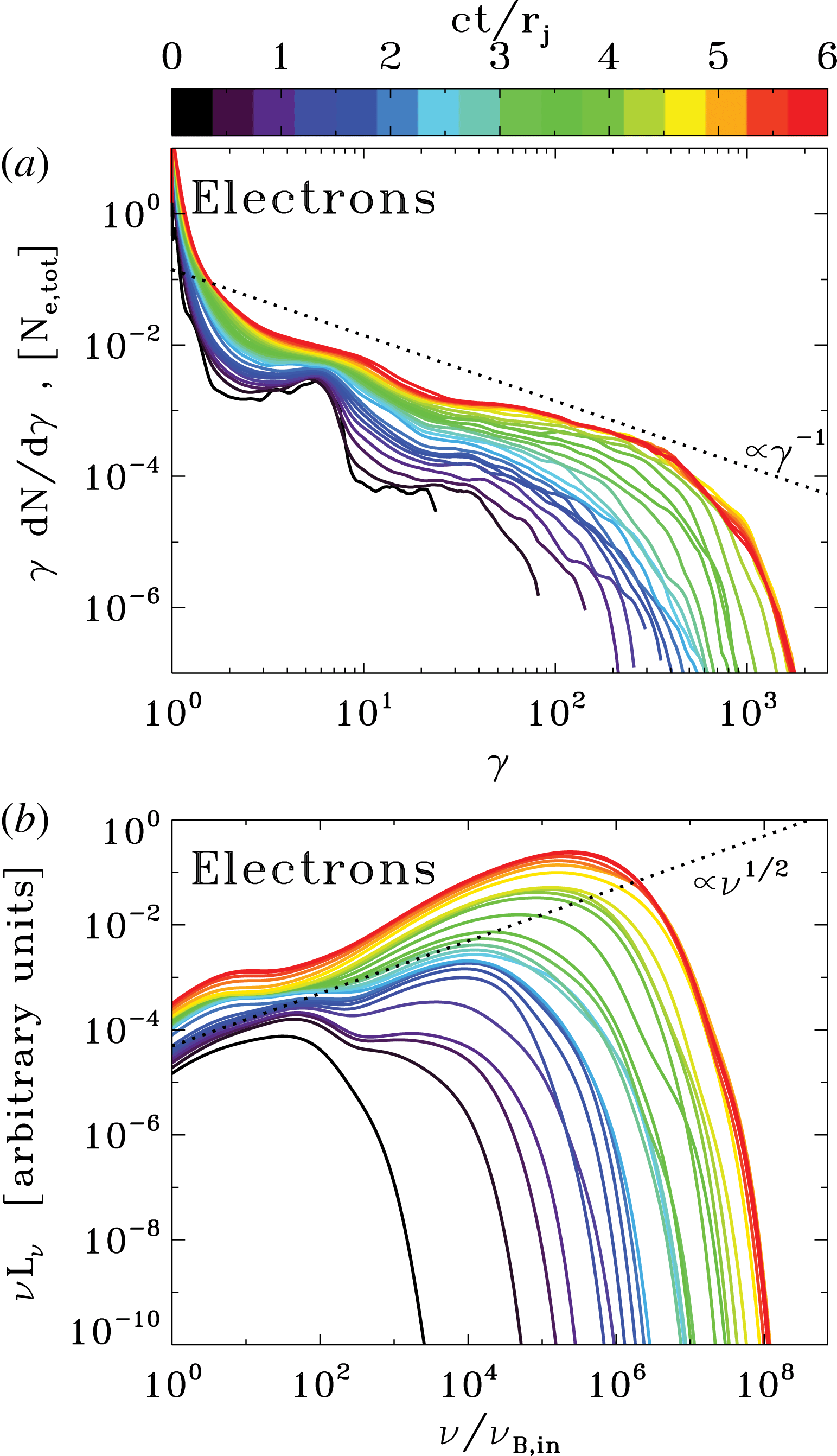
, see the colour bar at the top. (a) Evolution of the electron energy spectrum normalized to the total number of electrons. At late times, the spectrum approaches a distribution of the form
 $\unicode[STIX]{x1D6FE}\,\text{d}N/\text{d}\unicode[STIX]{x1D6FE}\propto \unicode[STIX]{x1D6FE}^{-1}$
, corresponding to equal energy content in each decade of
 $\unicode[STIX]{x1D6FE}$
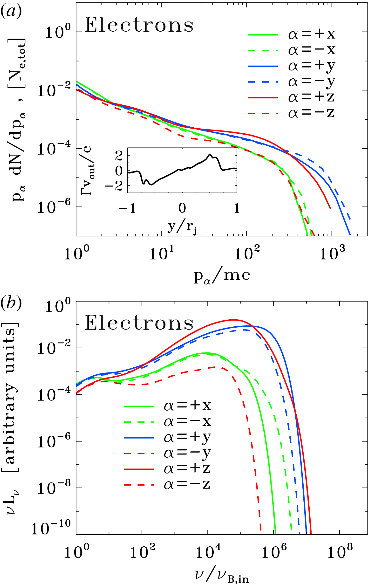
(compare with the dotted black line). The inset in (a) shows the electron momentum spectrum along different directions (as indicated in the legend), at the time when the electric energy peaks (as indicated by the dotted black line in figure 9). (b) Evolution of the angle-averaged synchrotron spectrum emitted by electrons. The frequency on the horizontal axis is normalized to
 $\unicode[STIX]{x1D708}_{B,in}=\sqrt{\unicode[STIX]{x1D70E}_{in}}\unicode[STIX]{x1D714}_{p}/2\unicode[STIX]{x03C0}$
. At late times, the synchrotron spectrum approaches
 $\unicode[STIX]{x1D708}L_{\unicode[STIX]{x1D708}}\propto \unicode[STIX]{x1D708}^{1/2}$
(compare with the dotted black line), which just follows from the electron spectrum
 $\unicode[STIX]{x1D6FE}\,\text{d}N/\text{d}\unicode[STIX]{x1D6FE}\propto \unicode[STIX]{x1D6FE}^{-1}$
. The inset in (b) shows the synchrotron spectrum at the time indicated in figure 9 (dotted black line) along different directions (within a solid angle of
 $\unicode[STIX]{x0394}\unicode[STIX]{x1D6FA}/4\unicode[STIX]{x03C0}\sim 3\times 10^{-3}$
), as indicated in the legend in the inset of (a). The resulting isotropy of the synchrotron emission is consistent with the particle distribution illustrated in the inset of (a).

2.4.2 Particle acceleration and emission signatures
The evolution of the particle spectrum in figure 10(a) illustrates the acceleration capabilities of the instability of ABC structures. Until
 $ct/L\sim 4$
, the particle spectrum does not show any sign of evolution, and it does not deviate from the initial Maxwellian distribution peaking at
 $\unicode[STIX]{x1D6FE}_{th}\simeq 300$
. From
 $ct/L\sim 4$
up to
 $ct/L\sim 8$
(from purple to light blue in the plot), the high-energy end of the particle spectrum undergoes a dramatic evolution, whereas the thermal peak is still unaffected (so, only a small fraction of the particles are accelerated). This is the most dramatic phase of particle acceleration, which we associate with the Crab flares. At the end of this explosive phase, the high-energy tail of the particle spectrum resembles a power law
 $\text{d}N/\text{d}\unicode[STIX]{x1D6FE}\propto \unicode[STIX]{x1D6FE}^{-s}$
with a hard slope
 $s\sim 1.5$
. The angle-averaged synchrotron spectrum (figure 10
b) parallels the extreme evolution of the particle spectrum, with the peak frequency of
 $\unicode[STIX]{x1D708}L_{\unicode[STIX]{x1D708}}$
moving from the ‘thermal’ value
 ${\sim}10^{8}\unicode[STIX]{x1D708}_{B,in}$
(dominated by the emission of thermal particles with
 $\unicode[STIX]{x1D6FE}\sim \unicode[STIX]{x1D6FE}_{th}$
) up to
 ${\sim}10^{13}\unicode[STIX]{x1D708}_{B,in}$
within just a few dynamical times. Here, we have defined
 $\unicode[STIX]{x1D708}_{B,in}=\sqrt{\unicode[STIX]{x1D70E}_{in}}\unicode[STIX]{x1D714}_{p}/2\unicode[STIX]{x03C0}$
.
The evolution at later times, during subsequent merger episodes, is at most moderate. From
 $ct/L\sim 8$
up to the final time
 $ct/L\sim 20$
(from light blue to red in the plot), the upper energy cutoff of the particle spectrum only increases by a factor of three, and the peak synchrotron frequency only by a factor of ten. The most significant evolution of the electron spectrum at such late times involves the thermal peak of the distribution, which shifts up in energy by a factor of
 ${\sim}10$
. This confirms what we have anticipated above, i.e. that subsequent episodes of island mergers primarily result in particle heating, rather than non-thermal acceleration. At the final time, the particle high-energy spectrum resembles a power law
 $\unicode[STIX]{x1D6FE}\,\text{d}N/\text{d}\unicode[STIX]{x1D6FE}\propto \unicode[STIX]{x1D6FE}^{-1}$
(compare with the dotted black line in a) and, consequently, the angle-averaged synchrotron spectrum approaches
 $\unicode[STIX]{x1D708}L_{\unicode[STIX]{x1D708}}\propto \unicode[STIX]{x1D708}^{1/2}$
(compare with the dotted black line in b).
The inset in figure 10(a) shows the electron momentum distribution along different directions (as indicated in the legend), at the time when the electric energy peaks (as indicated by the dotted black line in figure 9). The electron distribution is roughly isotropic. This might appear surprising, since at this time the particles are being dramatically accelerated at the collapsing X-points in between neighbouring islands, and in Paper I we have demonstrated that the particle distribution during X-point collapse is highly anisotropic. The accelerated electrons were beamed along the reconnection outflow and in the direction opposite to the accelerating electric field (while positrons were parallel to the electric field). Indeed, the particle distribution at each X-point in the collapsing ABC structure shows the same anisotropy as for a solitary X-point.
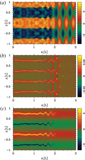
The apparent isotropy in the inset of figure 10(a) is a peculiar result of the ABC geometry. Figure 8(c) shows that in the
 $x{-}y$
plane the number of current sheets (and so, of reconnection outflows) oriented along
 $x$
is roughly comparable to those along
 $y$
. So, no preferred direction for the electron momentum spectrum is expected in the
 $x{-}y$
plane. In addition, in 2-D ABC structures the accelerating electric field
 $E_{z}$
has always the same polarity as the local out-of-plane magnetic field
 $B_{z}$
(or equivalently,
 $\boldsymbol{E}\boldsymbol{\cdot }\boldsymbol{B}>0$
at X-points, as we explicitly show in figure 12
c). In other words, current sheets that are coloured in yellow in figure 8(c) have
 $E_{z}>0$
, whereas
 $E_{z}<0$
in current sheets coloured in blue. Since the two options occur in equal numbers, no difference between the electron momentum spectrum in the
 $+z$
versus
 $-z$
direction is expected. Both the spatially integrated electron momentum distribution (inset in a) and the resulting synchrotron emission (inset in b) will then be nearly isotropic, for the case of ABC collapse.
Figures 11 and 12 describe the physics of particle acceleration during the instability of ABC structures. We consider a representative simulation with
 $kT/mc^{2}=10^{-4}$
,
 $\unicode[STIX]{x1D70E}_{in}=42$
and
 $L=251\,r_{L,\text{hot}}$
, performed within a square domain of size
 $2L\times 2L$
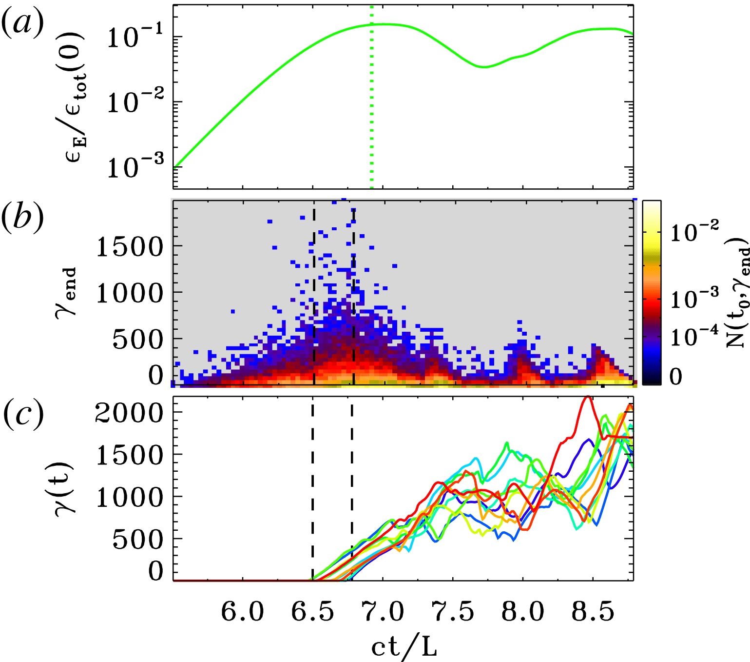
. In figure 11(b), we present a 2-D histogram of accelerated particles. On the vertical axis we plot the final particle Lorentz factor
 $\unicode[STIX]{x1D6FE}_{\text{end}}$
(measured at
 $ct/L=8.8$
), while the horizontal axis shows the particle injection time
 $ct_{0}/L$
, when the particle Lorentz factor first exceeded the threshold
 $\unicode[STIX]{x1D6FE}_{0}=30$
of our choice. The histogram shows that the particles that eventually reach the highest energies are injected into the acceleration process around
 $6.5\leqslant ct_{0}/L\leqslant 6.8$
(the two boundaries are indicated with vertical dashed black lines in b,c). For our simulation, this interval corresponds to the most violent stage of ABC instability, and it shortly precedes the time when the electric energy peaks (see the dotted green line in figure 11
a) and the current sheets reach their maximum length
 ${\sim}L$
.Footnote
3
In order to reach the highest energies, the accelerated particles should sample the full available potential of the current sheet, by exiting the reconnection layer when it reaches its maximal extent. Since they move at the speed of light along the sheet half-length
 ${\sim}0.5L$
, one can estimate that they should have been injected
 ${\sim}0.5L/c$
earlier than the peak time of the electric field. This is indeed in agreement with figure 11 (compare (a) and (b)).
Physics of particle acceleration, from a 2-D PIC simulation of ABC instability with
 $kT/mc^{2}=10^{-4}$
,
 $\unicode[STIX]{x1D70E}_{in}=42$
and
 $L=251\,r_{L,\text{hot}}$
, performed within a square domain of size
 $2L\times 2L$
. (a) Temporal evolution of the electric energy, in units of the total energy at the initial time. The dotted green vertical line marks the time when the electric energy peaks. (b) 2-D histogram of accelerated particles, normalized to the total number of particles. On the vertical axis we plot the final particle Lorentz factor
 $\unicode[STIX]{x1D6FE}_{\text{end}}$
(measured at the final time
 $ct/L=8.8$
), while the horizontal axis shows the particle injection time
 $ct_{0}/L$
, when the particle Lorentz factor first exceeded the threshold
 $\unicode[STIX]{x1D6FE}_{0}=30$
. (c) We select all the particles that exceed the threshold
 $\unicode[STIX]{x1D6FE}_{0}=30$
within a given time interval (chosen to be
 $6.5\leqslant ct_{0}/L\leqslant 6.8$
, as indicated by the vertical dashed black lines in b,c), and we plot the temporal evolution of the Lorentz factor of the ten particles that at the final time reach the highest energies.

Physics of particle injection into the acceleration process, from a 2-D PIC simulation of ABC instability with
 $kT/mc^{2}=10^{-4}$
,
 $\unicode[STIX]{x1D70E}_{in}=42$
and
 $L=251\,r_{L,\text{hot}}$
, performed within a square domain of size
 $2L\times 2L$
(same run as in figure 11). We plot the 2-D ABC structure at
 $ct/L=6.65$
. (a) Two-dimensional plot of the out-of-plane field
 $B_{z}$
, in units of
 $B_{0,in}$
. Among the particles that exceed the threshold
 $\unicode[STIX]{x1D6FE}_{0}=30$
within the interval
 $6.5\leqslant ct_{0}/L\leqslant 6.8$
(as indicated by the vertical dashed black lines in figure 11
b,c), we select the 20 particles that at the final time reach the highest energies, and with open white circles we plot their locations at the injection time
 $t_{0}$
. (b) Two-dimensional plot of the mean kinetic energy per particle
 $\langle \unicode[STIX]{x1D6FE}-1\rangle$
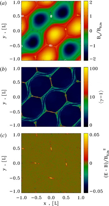
. (c) Two-dimensional plot of
 $\boldsymbol{E}\boldsymbol{\cdot }\boldsymbol{B}/B_{0,in}^{2}$
, showing in red and yellow the regions of charge starvation. Comparison of (a) and (c) shows that particle injection is localized in the charge-starved regions.

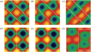
Snapshots of the numerical experiment demonstrating development of different modes of instability of 2-D ABC structures. (a–c) Parallel mode. White line, separating different layers are added as a guide. These pictures clearly demonstrate that during the development of the instability two layers of magnetic islands are shifting with respect to each other. (c,f) The compression mode. The white box demonstrates that a pair of aligned currents periodically approach each other.

Among the particles injected within
 $6.5\leqslant ct_{0}/L\leqslant 6.8$
, figure 11(c) shows the energy evolution of the ten positrons that reach the highest energies. We observe two distinct phases: an initial stage of direct acceleration by the reconnection electric field (at
 $6.5\lesssim ct/L\lesssim 7.3$
), followed by a phase of stochastic energy gains and losses (from
 $ct/L\sim 7.3$
up to the end). During the second stage, the pre-accelerated particles bounce off the wobbling/merging magnetic islands, and they further increase their energy via a second-order Fermi process (similar to what was observed by Hoshino Reference Hoshino2012). At the time of injection, the selected positrons were all localized in the vicinity of the collapsing X-points. This is shown in figure 12(a), where we plot with open white circles the location of the selected positrons at the time of injection, superimposed over the 2-D pattern of
 $B_{z}$
at
 $t\sim 6.65L/c$
. In the current sheets resulting from X-point collapse the force-free condition
 $\boldsymbol{E}\boldsymbol{\cdot }\boldsymbol{B}=0$
is violated (see the yellow regions in figure 12
c), so that they are sites of efficient particle acceleration (see also figure 12
b, showing the mean particle kinetic energy
 $\langle \unicode[STIX]{x1D6FE}-1\rangle$
).
2.4.3 Dependence on the flow parameters
In this subsection, we explore the dependence of our results on the initial plasma temperature, the in-plane magnetization
 $\unicode[STIX]{x1D70E}_{in}$
and the ratio
 $L/r_{L,\text{hot}}$
.
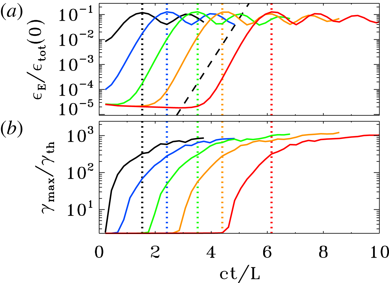
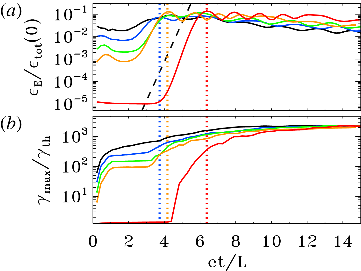
Figures 14 and 15 describes the dependence of our results on the flow temperature, for a suite of three simulations of ABC collapse with fixed
 $\unicode[STIX]{x1D70E}_{in}=42$
and fixed
 $L/r_{L,\text{hot}}=251$
, but different plasma temperatures:
 $kT/mc^{2}=10^{-4}$
(blue),
 $kT/mc^{2}=10$
(green) and
 $kT/mc^{2}=10^{2}$
(red). The definitions of both the in-plane magnetization
 $\unicode[STIX]{x1D70E}_{in}$
and the plasma skin depth
 $\,c/\unicode[STIX]{x1D714}_{p}$
(and so, also the Larmor radius
 $r_{L,\text{hot}}$
) account for the flow temperature, as described above. With this choice, figures 14 and 15 demonstrate that our results do not appreciably depend on the plasma temperature, apart from an overall shift in the energy scale. In particular, in the relativistic regime
 $kT/mc^{2}\gg 1$
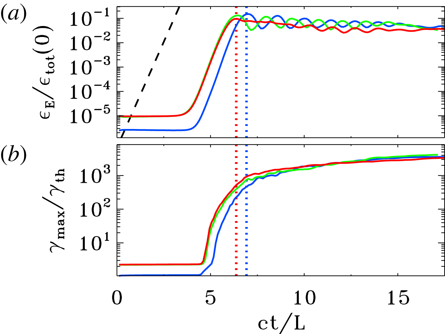
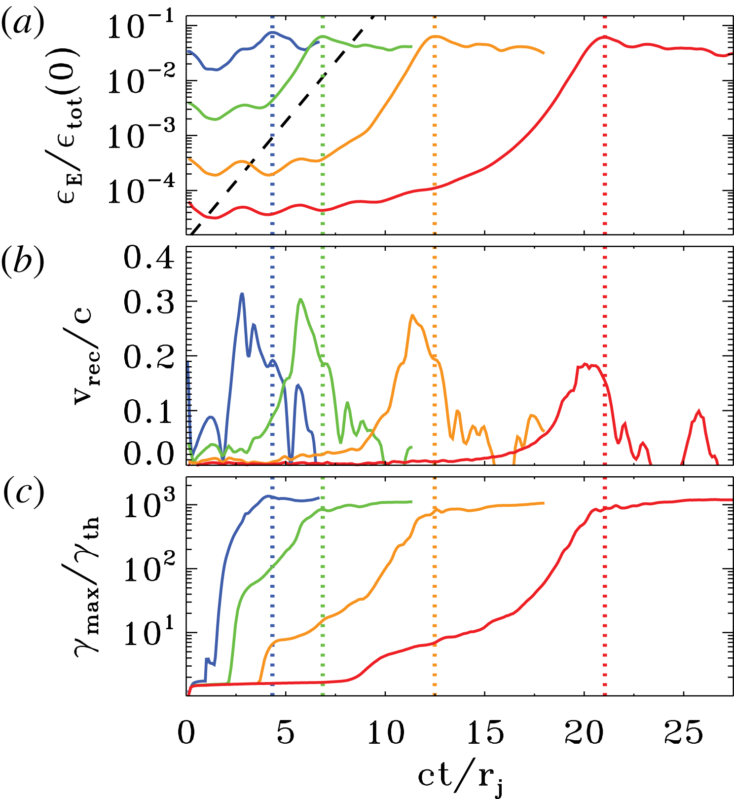
, our results for different temperatures are virtually indistinguishable. The onset of the ABC instability is nearly the same for the three values of temperature we investigate (figure 14
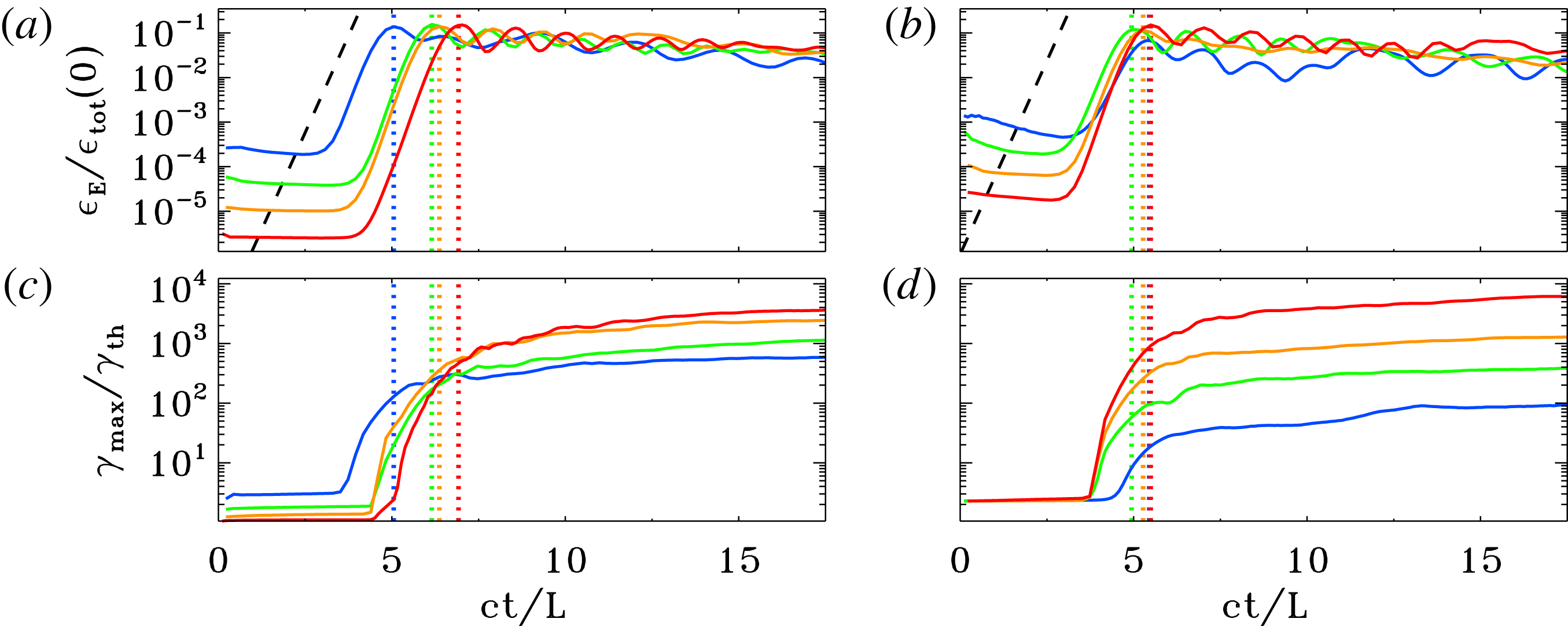
a), the exponential growth is the same (with a rate equal to
 ${\sim}4c/L$
for the electric energy, compare with the dashed black line) and the peak time is quite similar (with a minor delay for the non-relativistic case
 $kT/mc^{2}=10^{-4}$
, in blue). At the onset of the ABC instability, the upper cutoff
 $\unicode[STIX]{x1D6FE}_{\text{max}}$
of the particle energy spectrum grows explosively. Once normalized to the thermal value
 $\unicode[STIX]{x1D6FE}_{th}\simeq 1+(\hat{\unicode[STIX]{x1D6FE}}-1)^{-1}kT/mc^{2}$
(which equals
 $\unicode[STIX]{x1D6FE}_{th}\simeq 1$
for
 $kT/mc^{2}\ll 1$
and
 $\unicode[STIX]{x1D6FE}_{th}\simeq 3kT/mc^{2}$
for
 $kT/mc^{2}\gg 1$
), the temporal evolution of
 $\unicode[STIX]{x1D6FE}_{\text{max}}$
does not appreciably depend on the initial temperature, especially in the relativistic regime
 $kT/mc^{2}\gg 1$
(green and red lines).
Temporal evolution of the electric energy (a; in units of the total initial energy) and of the maximum particle Lorentz factor (b;
 $\unicode[STIX]{x1D6FE}_{\text{max}}$
is defined in (2.3), and it is normalized to the thermal Lorentz factor
 $\unicode[STIX]{x1D6FE}_{th}\simeq 1+(\hat{\unicode[STIX]{x1D6FE}}-1)^{-1}kT/mc^{2}$
), for a suite of three PIC simulations of ABC collapse with fixed
 $\unicode[STIX]{x1D70E}_{in}=42$
and fixed
 $L/r_{L,\text{hot}}=251$
, but different plasma temperatures:
 $kT/mc^{2}=10^{-4}$
(blue),
 $kT/mc^{2}=10$
(green) and
 $kT/mc^{2}=10^{2}$
(red). The dashed black line in (a) shows that the electric energy grows exponentially as
 $\propto \exp (4ct/L)$
. The vertical dotted lines mark the time when the electric energy peaks (colours correspond to the three values of
 $kT/mc^{2}$
, as described above).

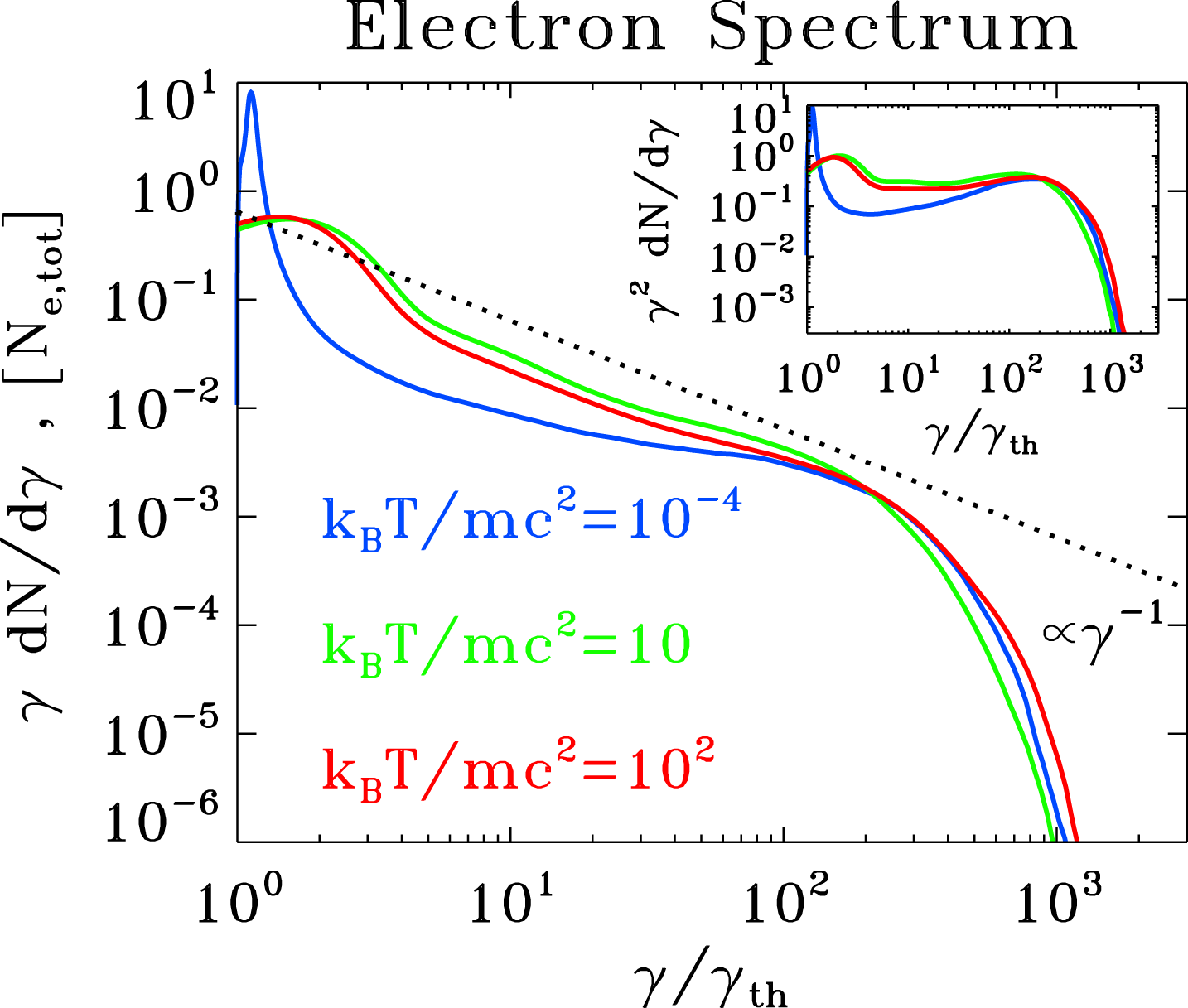
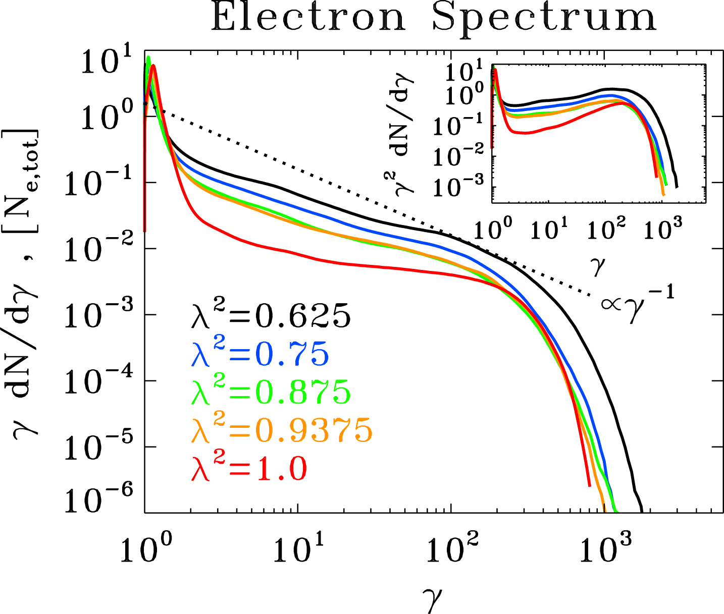
Particle spectrum at the time when the electric energy peaks, for a suite of three PIC simulations of ABC collapse with fixed
 $\unicode[STIX]{x1D70E}_{in}=42$
and fixed
 $L/r_{L,\text{hot}}=251$
, but different plasma temperatures:
 $kT/mc^{2}=10^{-4}$
(blue),
 $kT/mc^{2}=10$
(green) and
 $kT/mc^{2}=10^{2}$
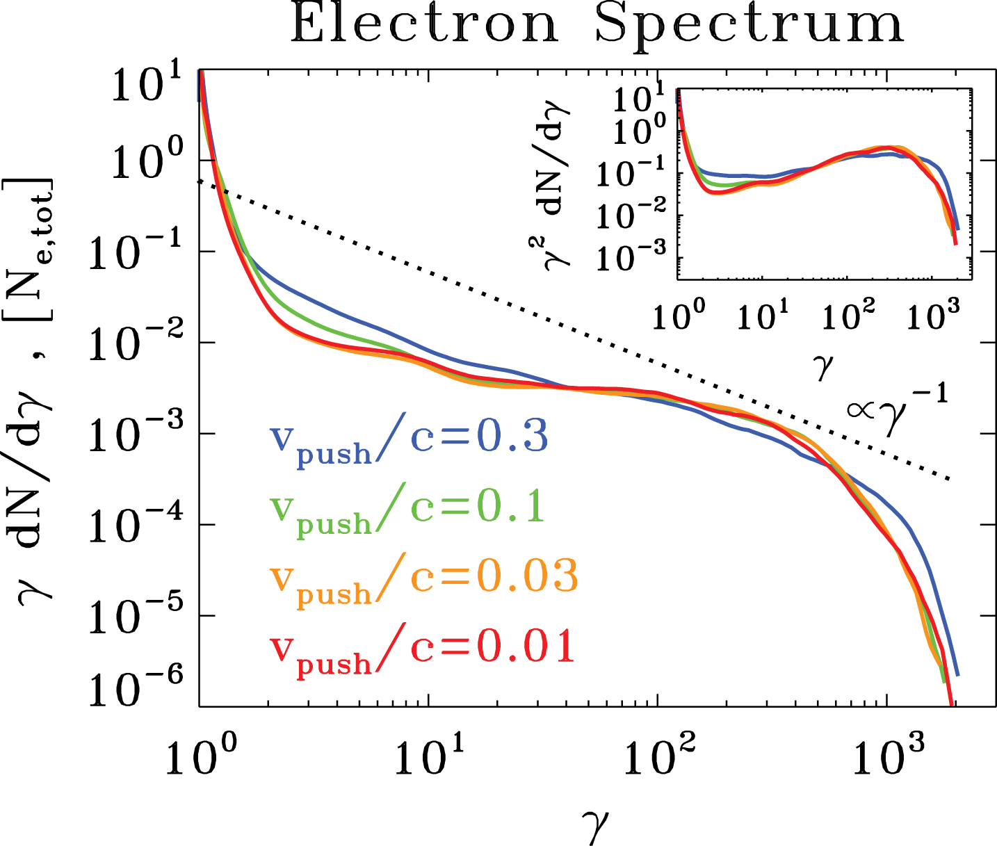
(red). The main plot shows
 $\unicode[STIX]{x1D6FE}\,\text{d}N/\text{d}\unicode[STIX]{x1D6FE}$
to emphasize the particle content, whereas the inset presents
 $\unicode[STIX]{x1D6FE}^{2}\,\text{d}N/\text{d}\unicode[STIX]{x1D6FE}$
to highlight the energy census. The dotted black line is a power law
 $\unicode[STIX]{x1D6FE}\,\text{d}N/\text{d}\unicode[STIX]{x1D6FE}\propto \unicode[STIX]{x1D6FE}^{-1}$
, corresponding to equal energy content per decade (which would result in a flat distribution in the inset). The particle Lorentz factor on the horizontal axis is normalized to the thermal value
 $\unicode[STIX]{x1D6FE}_{th}$
, to facilitate comparison among the three cases.

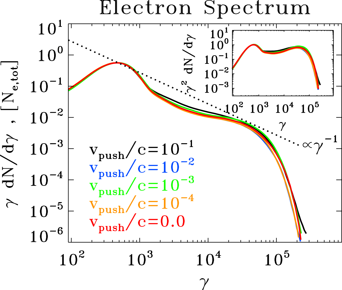
Similar conclusions hold for the particle spectrum
 $\unicode[STIX]{x1D6FE}\,\text{d}N/\text{d}\unicode[STIX]{x1D6FE}$
at the time when the electric energy peaks, presented in the main panel of figure 15. The spectra of
 $kT/mc^{2}=10$
(green) and
 $kT/mc^{2}=10^{2}$
(red) overlap, once the horizontal axis is normalized to the thermal Lorentz factor
 $\unicode[STIX]{x1D6FE}_{th}$
. Their high-energy end approaches the slope
 $\unicode[STIX]{x1D6FE}\,\text{d}N/\text{d}\unicode[STIX]{x1D6FE}\propto \unicode[STIX]{x1D6FE}^{-1}$
indicated with the dotted black line. This corresponds to a distribution with equal energy content per decade (which would result in a flat distribution in the inset, where we plot
 $\unicode[STIX]{x1D6FE}^{2}\text{d}N/\text{d}\unicode[STIX]{x1D6FE}$
to emphasize the energy census). The spectrum for
 $kT/mc^{2}=10^{-4}$
(blue line) is marginally harder, but its high-energy part is remarkably similar.
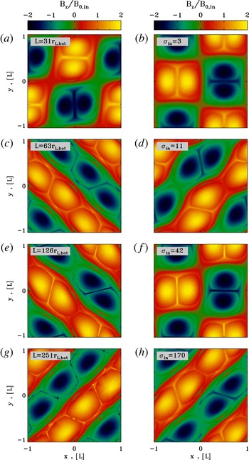
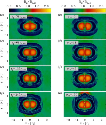
Two-dimensional pattern of the out-of-plane field
 $B_{z}$
(in units of
 $B_{0,in}$
) at the most violent time of ABC instability (i.e. when the electric energy peaks, as indicated by the vertical dotted lines in figure 17) from a suite of PIC simulations. In (a,c,e,g), we fix
 $kT/mc^{2}=10^{-4}$
and
 $\unicode[STIX]{x1D70E}_{in}=42$
and we vary the ratio
 $L/r_{L,\text{hot}}$
, from 31 to 251 (from top to bottom). In (b,d,f,h), we fix
 $kT/mc^{2}=10^{2}$
and
 $L/r_{L,\text{hot}}=63$
and we vary the magnetization
 $\unicode[STIX]{x1D70E}_{in}$
, from 3 to 170 (from top to bottom). In all cases, the domain is a square of size
 $2L\times 2L$
. The 2-D structure of
 $B_{z}$
in all cases is quite similar, apart from the fact that larger
 $L/r_{L,\text{hot}}$
tend to lead to a more pronounced fragmentation of the current sheet. Some cases go unstable via the ‘parallel’ mode depicted in figure 3, others via the ‘oblique’ mode described in figure 2.

We now investigate the dependence of our results on the magnetization
 $\unicode[STIX]{x1D70E}_{in}$
and the ratio
 $L/r_{L,\text{hot}}$
, where
 $r_{L,\text{hot}}=\sqrt{\unicode[STIX]{x1D70E}_{in}}\,c/\unicode[STIX]{x1D714}_{p}$
. In figure 16, we present the 2-D pattern of the out-of-plane field
 $B_{z}$
(in units of
 $B_{0,in}$
) at the most violent time of ABC instability (i.e. when the electric energy peaks, as indicated by the vertical dotted lines in figure 17) from a suite of PIC simulations in a square domain
 $2L\times 2L$
. In (a,c,e,g), we fix
 $kT/mc^{2}=10^{-4}$
and
 $\unicode[STIX]{x1D70E}_{in}=42$
and we vary the ratio
 $L/r_{L,\text{hot}}$
, from 31 to 251 (from top to bottom). In (b,d,f,h), we fix
 $kT/mc^{2}=10^{2}$
and
 $L/r_{L,\text{hot}}=63$
and we vary the magnetization
 $\unicode[STIX]{x1D70E}_{in}$
, from 3 to 170 (from top to bottom). The figure shows that the instability proceeds in a similar way in all the runs, even though some cases go unstable via the ‘parallel’ mode depicted in figure 3 (e.g. see the top right panel), others via the ‘oblique’ mode described in figure 2 (e.g. see the bottom left panel). Here, ‘parallel’ and ‘oblique’ refer to the orientation of the wavevector with respect to the axes of the box.
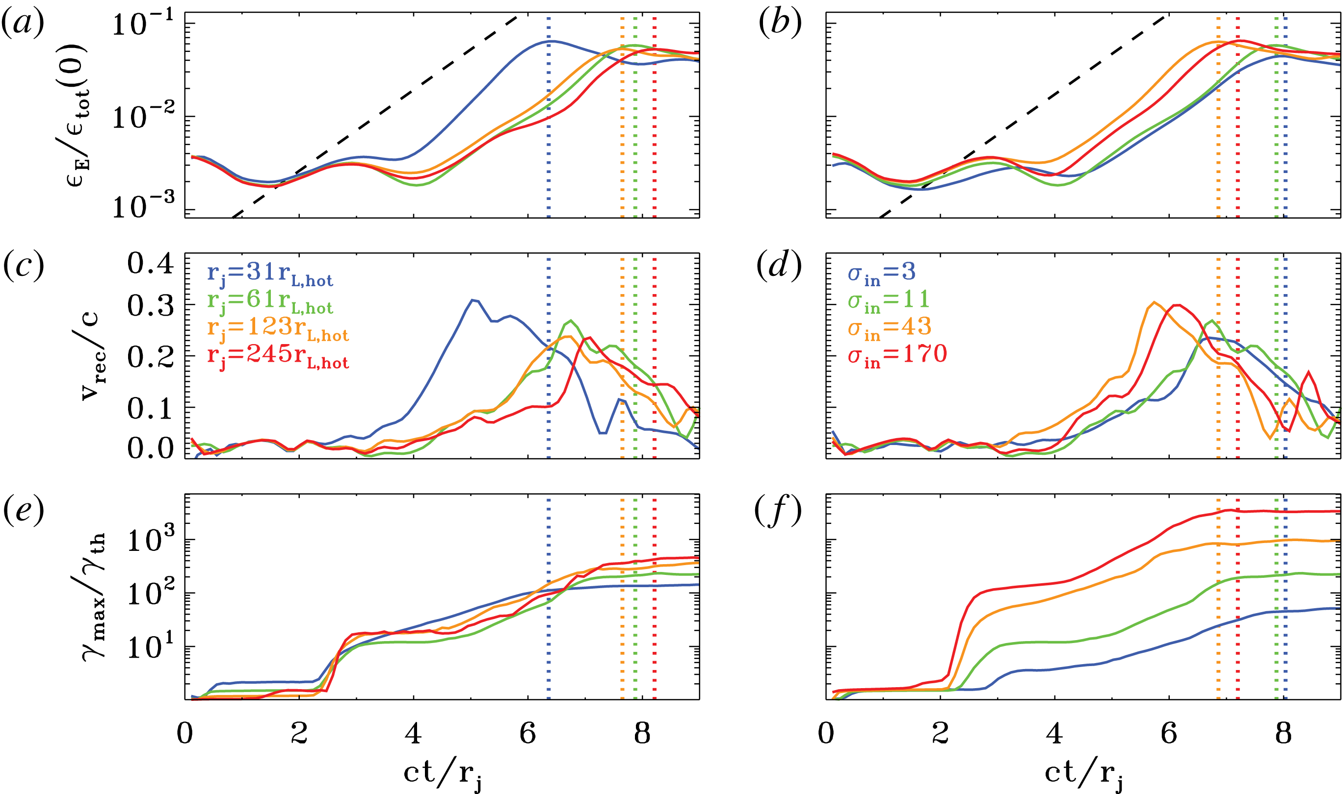
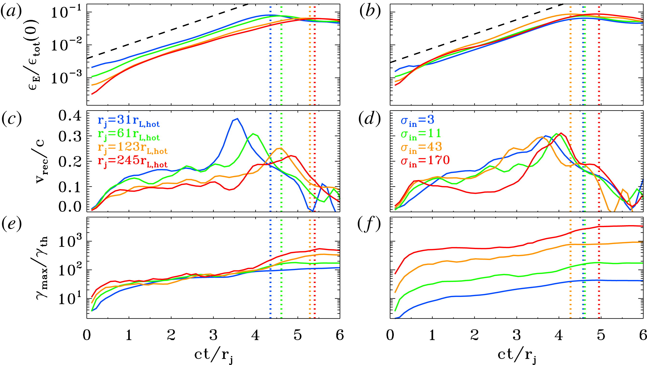
Temporal evolution of the electric energy (a,b; in units of the total initial energy) and of the maximum particle Lorentz factor (c,d;
 $\unicode[STIX]{x1D6FE}_{\text{max}}$
is defined in (2.3), and it is normalized to the thermal Lorentz factor
 $\unicode[STIX]{x1D6FE}_{th}\simeq 1+(\hat{\unicode[STIX]{x1D6FE}}-1)^{-1}kT/mc^{2}$
), for a suite of PIC simulations of ABC collapse (same runs as in figure 16). In (a,c), we fix
 $kT/mc^{2}=10^{-4}$
and
 $\unicode[STIX]{x1D70E}_{in}=42$
and we vary the ratio
 $L/r_{L,\text{hot}}$
from 31 to 251 (from blue to red). In (b,d), we fix
 $kT/mc^{2}=10^{2}$
and
 $L/r_{L,\text{hot}}=63$
and we vary the magnetization
 $\unicode[STIX]{x1D70E}_{in}$
from 3 to 170 (from blue to red). The maximum particle energy resulting from ABC collapse increases for increasing
 $L/r_{L,\text{hot}}$
at fixed
 $\unicode[STIX]{x1D70E}_{in}$
(a,c) and for increasing
 $\unicode[STIX]{x1D70E}_{in}$
at fixed
 $L/r_{L,\text{hot}}$
. The dashed black line in (a,c) shows that the electric energy grows exponentially as
 $\propto \exp (4ct/L)$
. The vertical dotted lines mark the time when the electric energy peaks (colours as described above).

The evolution is remarkably similar, whether the instability proceeds via the parallel or the oblique mode. Yet, some differences can be found: (i) in the oblique mode, all the null points are activated, i.e. they all evolve into a long thin current sheet suitable for particle acceleration; in contrast, in the parallel mode only half of the null points are activated (e.g. the null point at
 $x=0$
and
 $y=0.5L$
in the top right panel does not form a current sheet, and we have verified that it does not lead to significant particle acceleration). Everything else being equal, this results in a difference by a factor of two in the normalization of the high-energy tail of accelerated particles (i.e. the acceleration efficiency differs by a factor of two), as we have indeed verified. (ii) The current sheets of the parallel mode tend to stretch longer than for the oblique mode (by approximately a factor of
 $\sqrt{2}$
), resulting in a difference of a factor of
 $\sqrt{2}$
in the maximum particle energy, everything else being the same. (iii) In the explosive phase of the instability, the oblique mode tends to dissipate some fraction of the out-of-plane field energy (still, a minor fraction as compared to the dissipated in-plane energy), whereas the parallel mode does not. Regardless of such differences, both modes result in efficient particle acceleration and heating, and in a similar temporal evolution of the rate of magnetic energy dissipation (with the kinetic energy fraction reaching
 $\unicode[STIX]{x1D716}_{\text{kin}}/\unicode[STIX]{x1D716}_{\text{tot}}(0)\sim 0.1$
during the explosive phase, and eventually saturating at
 $\unicode[STIX]{x1D716}_{\text{kin}}/\unicode[STIX]{x1D716}_{\text{tot}}(0)\sim 0.5$
).
The 2-D pattern of
 $B_{z}$
shown in figure 16 shows a tendency for thinner current sheets at larger
 $L/r_{L,\text{hot}}$
, when fixing
 $\unicode[STIX]{x1D70E}_{in}$
(figure 16
a,c,e,g). Roughly, the thickness of the current sheet is set by the Larmor radius
 $r_{L,\text{hot}}$
of the high-energy particles heated/accelerated by reconnection. In (b,d,f,h), with
 $L/r_{L,\text{hot}}$
fixed, the thickness of the current sheet is then a fixed fraction of the box size. In contrast, in (a,c,e,g), the ratio of current sheet thickness to box size will scale as
 $r_{L,\text{hot}}/L$
, as indeed it is observed. A long thin current sheet is expected to fragment into a chain of plasmoids/magnetic islands (e.g. Uzdensky et al.
Reference Uzdensky, Loureiro and Schekochihin2010; Werner et al.
Reference Werner, Uzdensky, Cerutti, Nalewajko and Begelman2016), when the length-to-thickness ratio is much larger than unity.Footnote
4
It follows that the cases in (b,d,f,h) will display a similar tendency for fragmentation (and in particular, they do not appreciably fragment), whereas the likelihood of fragmentation is expected to increase from top to bottom in (a,c,e,g). In fact, for the case with
 $L/r_{L,\text{hot}}=251$
(g), a number of small-scale plasmoids appear in the current sheets (e.g. see the plasmoid at
 $x=0$
and
 $y=-0.5L$
in g). We find that as long as
 $\unicode[STIX]{x1D70E}_{in}\gg 1$
, the secondary tearing mode discussed by Uzdensky et al. (Reference Uzdensky, Loureiro and Schekochihin2010) – that leads to current sheet fragmentation – appears at
 $L/r_{L,\text{hot}}\gtrsim 200$
, in the case of ABC collapse.Footnote
5
In addition to the runs presented in figure 16, we have confirmed this result by covering the whole
 $\unicode[STIX]{x1D70E}_{in}-L/r_{L,\text{hot}}$
parameter space, with
 $\unicode[STIX]{x1D70E}_{in}$
from 3 to 680 and with
 $L/r_{L,\text{hot}}$
from 31 to 502.
We have performed an additional test to check that the current sheet thickness scales as
 $r_{L,\text{hot}}$
. When the reconnection layers reach their maximal extent (i.e. at the peak of the electric energy), the current sheet length should scale as
 $L$
, whereas its thickness should be
 ${\sim}r_{L,\text{hot}}$
. Since the current sheets are characterized by a field-aligned electric field (figure 12
c), the fraction of box area occupied by regions with
 $\boldsymbol{E}\boldsymbol{\cdot }\boldsymbol{B}\neq 0$
should scale as
 $r_{L,\text{hot}}/L$
. We have explicitly verified that this is indeed the case, both when comparing runs that have the same
 $L/r_{L,\text{hot}}$
and for simulations that keep
 $\unicode[STIX]{x1D70E}_{in}$
fixed.
The reconnection rate in all the cases we have explored is around
 $v_{\text{rec}}/c\sim 0.3-0.5$
. It shows a marginal tendency for decreasing with increasing
 $L/r_{L,\text{hot}}$
(but we have verified that it saturates at
 $v_{\text{rec}}/c\sim 0.3$
in the limit
 $L/r_{L,\text{hot}}\gg 1$
), and it moderately increases with
 $\unicode[STIX]{x1D70E}_{in}$
(especially as we transition from the non-relativistic regime to the relativistic regime, but it saturates at
 $v_{\text{rec}}/c\sim 0.5$
in the limit
 $\unicode[STIX]{x1D70E}_{in}\gg 1$
). Our measurements of the inflow speed (which we take as a proxy for the reconnection rate) are easier when the parallel mode dominates, since the inflow direction lies along one of the Cartesian axes, rather than for the oblique mode. In simulations with an aspect ratio of
 $2L\times L$
, the parallel mode is the only one that gets triggered, and most of the measurements quoted above refer to this set-up.
In figure 17 we present the temporal evolution of the runs whose 2-D structure is shown in figure 16. In (a,c), we fix
 $kT/mc^{2}=10^{-4}$
and
 $\unicode[STIX]{x1D70E}_{in}=42$
and we vary the ratio
 $L/r_{L,\text{hot}}$
from 31 to 251 (from blue to red). In (b,d), we fix
 $kT/mc^{2}=10^{2}$
and
 $L/r_{L,\text{hot}}=63$
and we vary the magnetization
 $\unicode[STIX]{x1D70E}_{in}$
from 3 to 170 (from blue to red). (a,b) Show that the evolution of the electric energy (in units of the total initial energy) is remarkably similar for all the values of
 $L/r_{L,\text{hot}}$
and
 $\unicode[STIX]{x1D70E}_{in}$
we explore. In particular, the electric energy grows as
 $\propto \exp (4ct/L)$
in all the cases (see the dashed black lines), and it peaks at
 ${\sim}10\,\%$
of the total initial energy. The only exception is the trans-relativistic case
 $\unicode[STIX]{x1D70E}_{in}=3$
and
 $L/r_{L,\text{hot}}=63$
(blue line in b), whose peak value is slightly smaller, due to the lower Alfvén speed. The onset time of the instability is also nearly independent of
 $\unicode[STIX]{x1D70E}_{in}$
(b), although the trans-relativistic case
 $\unicode[STIX]{x1D70E}_{in}=3$
(blue line) seems to be growing slightly later. As regard to the dependence of the onset time on
 $L/r_{L,\text{hot}}$
at fixed
 $\unicode[STIX]{x1D70E}_{in}$
, figure 17(a) shows that larger values of
 $L/r_{L,\text{hot}}$
tend to grow later, but the variation is only moderate: in all the cases the instability grows around
 $ct/L\sim 5$
.
In the early stages of ABC instability, the cutoff Lorentz factor
 $\unicode[STIX]{x1D6FE}_{\text{max}}$
of the particle energy spectrum (as defined in (2.3)) grows explosively (see figure 17
c,d). If the origin of time is set at the onset time of the instability, the maximum energy is expected to grow as
 $$\begin{eqnarray}\unicode[STIX]{x1D6FE}_{\text{max}}mc^{2}\sim ev_{\text{rec}}B_{in}t\end{eqnarray}$$
Due to the approximate linear increase of the in-plane magnetic field with distance from a null point, we find that
 $B_{in}\propto \sqrt{\unicode[STIX]{x1D70E}_{in}}v_{\text{rec}}t/L$
. This leads to
 $\unicode[STIX]{x1D6FE}_{\text{max}}\propto v_{\text{rec}}^{2}\sqrt{\unicode[STIX]{x1D70E}_{in}}t^{2}/L$
, with the same quadratic temporal scaling that was discussed for the solitary X-point collapse. Since the dynamical phase of ABC instability lasts a few
 $L/c$
, the maximum particle Lorentz factor at the end of this stage should scale as
 $\unicode[STIX]{x1D6FE}_{\text{max}}\propto v_{\text{rec}}^{2}\sqrt{\unicode[STIX]{x1D70E}_{in}}L\propto v_{\text{rec}}^{2}\unicode[STIX]{x1D70E}_{in}(L/r_{L,\text{hot}})$
. If the reconnection rate does not significantly depend on
 $\unicode[STIX]{x1D70E}_{in}$
, this implies that
 $\unicode[STIX]{x1D6FE}_{\text{max}}\propto L$
at fixed
 $\unicode[STIX]{x1D70E}_{in}$
. The trend for an increasing
 $\unicode[STIX]{x1D6FE}_{\text{max}}$
with
 $L$
at fixed
 $\unicode[STIX]{x1D70E}_{in}$
is confirmed in figure 17(c), both at the final time and at the peak time of the electric energy (which is slightly different among the four different cases, see the vertical dotted coloured lines).Footnote
6
Similarly, if the reconnection rate does not significantly depend on
 $L/r_{L,\text{hot}}$
, this implies that
 $\unicode[STIX]{x1D6FE}_{\text{max}}\propto \unicode[STIX]{x1D70E}_{in}$
at fixed
 $L/r_{L,\text{hot}}$
. This linear dependence of
 $\unicode[STIX]{x1D6FE}_{\text{max}}$
on
 $\unicode[STIX]{x1D70E}_{in}$
is confirmed in figure 17(d).
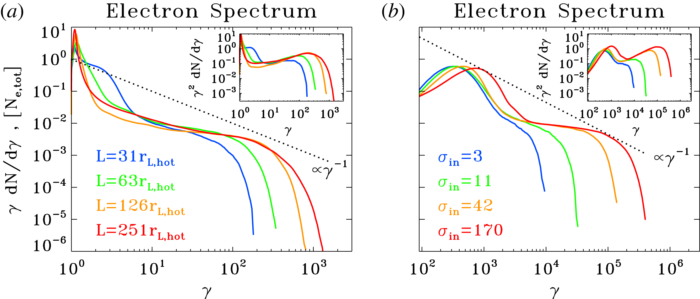
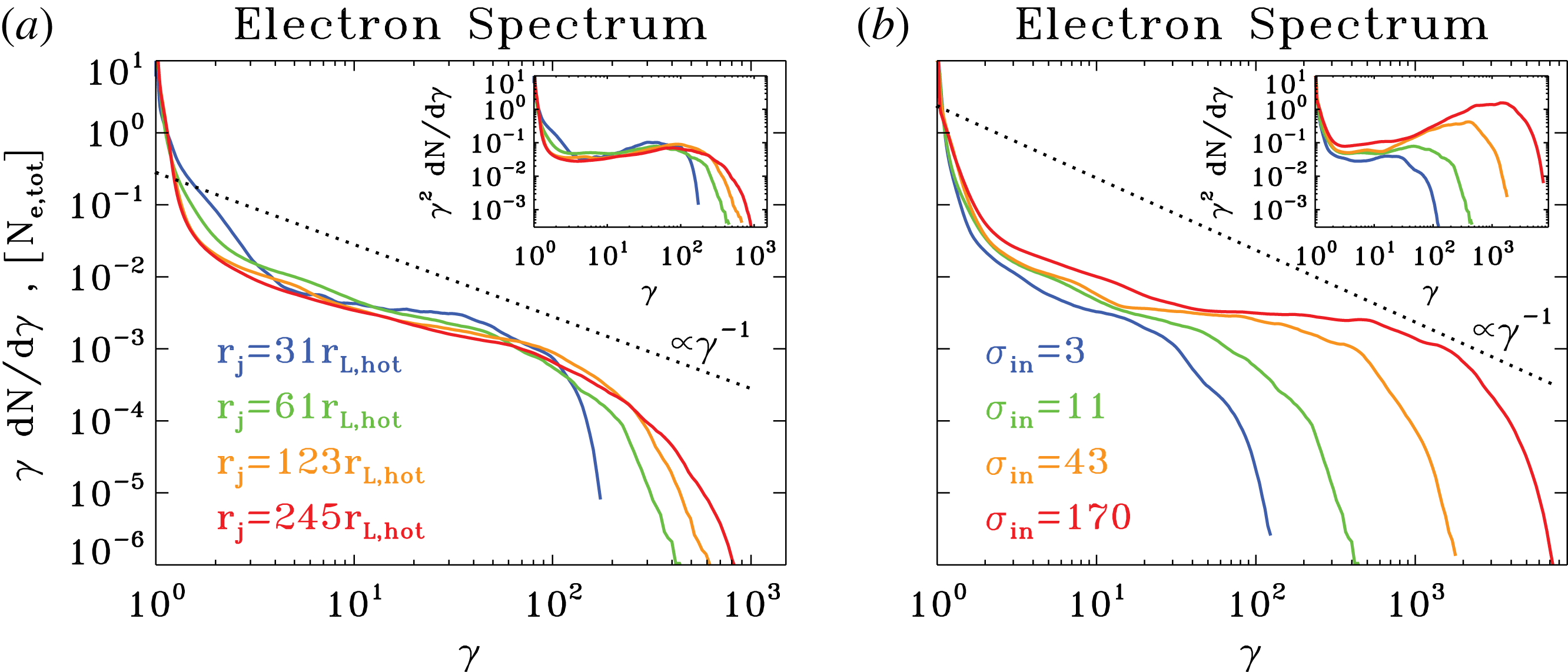
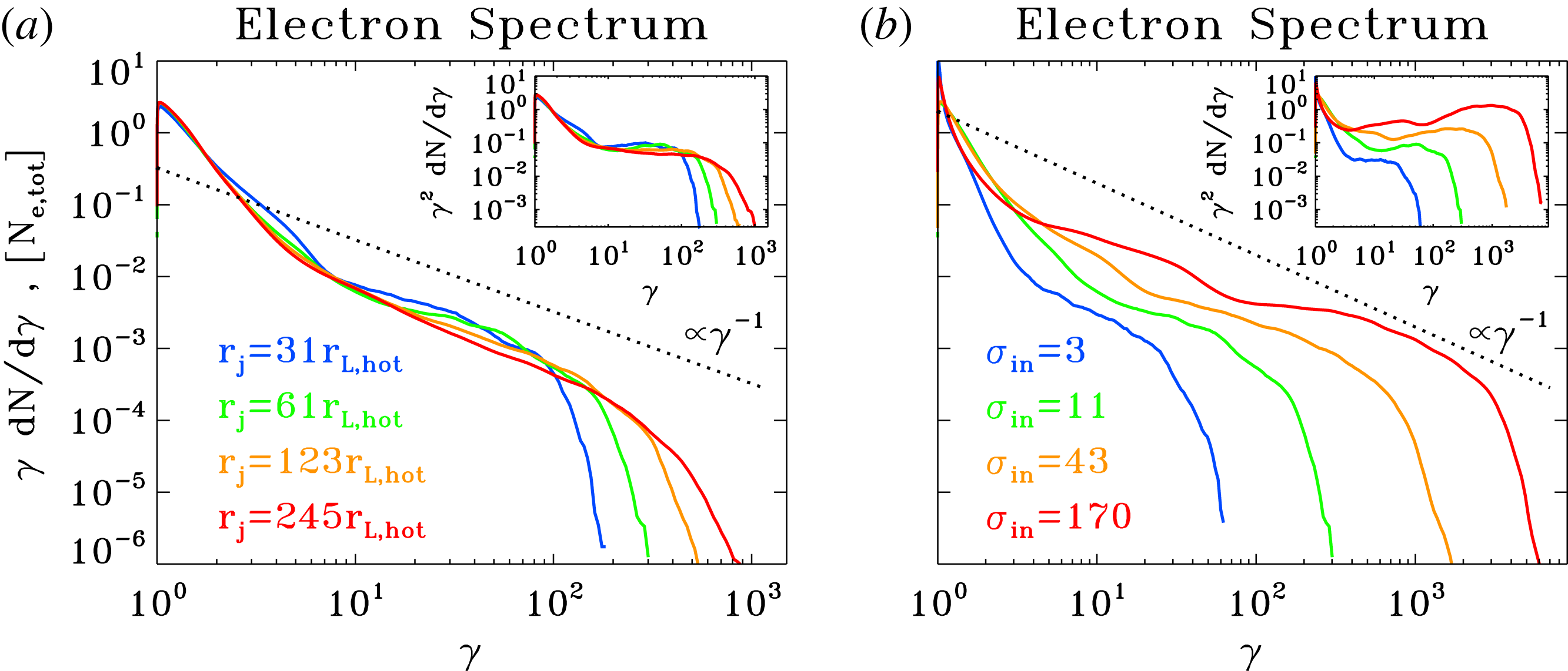
Particle spectrum at the time when the electric energy peaks, for a suite of PIC simulations of ABC collapse (same runs as in figures 16 and 17). In (a) we fix
 $kT/mc^{2}=10^{-4}$
and
 $\unicode[STIX]{x1D70E}_{in}=42$
and we vary the ratio
 $L/r_{L,\text{hot}}$
from 31 to 251 (from blue to red, as indicated by the legend). In (b) we fix
 $kT/mc^{2}=10^{2}$
and
 $L/r_{L,\text{hot}}=63$
and we vary the magnetization
 $\unicode[STIX]{x1D70E}_{in}$
from 3 to 170 (from blue to red, as indicated by the legend). The main plot shows
 $\unicode[STIX]{x1D6FE}\,\text{d}N/\text{d}\unicode[STIX]{x1D6FE}$
to emphasize the particle content, whereas the inset presents
 $\unicode[STIX]{x1D6FE}^{2}\,\text{d}N/\text{d}\unicode[STIX]{x1D6FE}$
to highlight the energy census. The dotted black line is a power law
 $\unicode[STIX]{x1D6FE}\,\text{d}N/\text{d}\unicode[STIX]{x1D6FE}\propto \unicode[STIX]{x1D6FE}^{-1}$
, corresponding to equal energy content per decade (which would result in a flat distribution in the insets). The spectral hardness is not a sensitive function of the ratio
 $L/r_{L,\text{hot}}$
, but it is strongly dependent on
 $\unicode[STIX]{x1D70E}_{in}$
, with higher magnetizations giving harder spectra, up to the saturation slope of
 $-1$
.

The dependence of the particle spectrum on
 $L/r_{L,\text{hot}}$
and
 $\unicode[STIX]{x1D70E}_{in}$
is illustrated in figure 18 ((a) and (b), respectively), where we present the particle energy distribution at the time when the electric energy peaks (as indicated by the coloured vertical dotted lines in figure 17). The particle spectrum shows a pronounced non-thermal component in all the cases, regardless of whether the secondary plasmoid instability is triggered or not in the current sheets (the results presented in figure 18 correspond to the cases displayed in figure 16). This suggests that in our set-up any acceleration mechanism that relies on plasmoid mergers is not very important, but rather that the dominant source of energy is direct acceleration by the reconnection electric field (see the previous subsection).
At the time when the electric energy peaks, most of the particles are still in the thermal component (at
 $\unicode[STIX]{x1D6FE}\sim 1$
in (a) and
 $\unicode[STIX]{x1D6FE}\sim 3kT/mc^{2}$
in figure 18
b), i.e. bulk heating is still negligible. Yet, a dramatic event of particle acceleration is taking place, with a few lucky particles accelerated much beyond the mean energy per particle
 ${\sim}\unicode[STIX]{x1D6FE}_{th}\unicode[STIX]{x1D70E}_{in}/2$
(for comparison, we point out that
 $\unicode[STIX]{x1D6FE}_{th}\sim 1$
and
 $\unicode[STIX]{x1D70E}_{in}=42$
for the cases in a). Since most of the particles are at the thermal peak, this is not violating energy conservation. As described by Sironi & Spitkovsky (Reference Sironi and Spitkovsky2014) and Werner et al. (Reference Werner, Uzdensky, Cerutti, Nalewajko and Begelman2016), for a power-law spectrum
 $\text{d}N/\text{d}\unicode[STIX]{x1D6FE}\propto \unicode[STIX]{x1D6FE}^{-p}$
of index
 $1<p<2$
extending from
 $\unicode[STIX]{x1D6FE}\sim \unicode[STIX]{x1D6FE}_{th}$
up to
 $\unicode[STIX]{x1D6FE}_{\text{max}}$
, the fact that the mean energy per particle is
 $\unicode[STIX]{x1D6FE}_{th}\unicode[STIX]{x1D70E}_{in}/2$
yields a constraint on the upper cutoff of the form
 $$\begin{eqnarray}\unicode[STIX]{x1D6FE}_{\text{max}}\lesssim \unicode[STIX]{x1D6FE}_{th}\left[\frac{\unicode[STIX]{x1D70E}_{in}}{2}\frac{2-p}{p-1}\right]^{1/(2-p)}.\end{eqnarray}$$
This constraint does not apply during the explosive phase, since most of the particles lie at the thermal peak (so, the distribution does not resemble a single power law), but it does apply at late times (e.g. see the final spectrum in figure 10, similar to a power law). However, as the bulk of the particles shift up to higher energies (see the evolution of the thermal peak in figure 10), the spectrum at late times tends to be softer than in the early explosive phase (compare light blue and red curves in figure 10), which helps relaxing the constraint in (2.3).
The spectra in figure 18 (main panels for
 $\unicode[STIX]{x1D6FE}\,\text{d}N/\text{d}\unicode[STIX]{x1D6FE}$
, to emphasize the particle content; insets for
 $\unicode[STIX]{x1D6FE}^{2}\,\text{d}N/\text{d}\unicode[STIX]{x1D6FE}$
, to highlight the energy census) confirm the trend of
 $\unicode[STIX]{x1D6FE}_{\text{max}}$
anticipated above. At fixed
 $\unicode[STIX]{x1D70E}_{in}=42$
(a), we see that
 $\unicode[STIX]{x1D6FE}_{\text{max}}\propto L$
(
 $L$
changes by a factor of two in between each pair of curves);Footnote
7
on the other hand, at fixed
 $L/r_{L,\text{hot}}=63$
(b), we find that
 $\unicode[STIX]{x1D6FE}_{\text{max}}\propto \unicode[STIX]{x1D70E}_{in}$
(
 $\unicode[STIX]{x1D70E}_{in}$
changes by a factor of four in between each pair of curves).
The spectral hardness is primarily controlled by the average in-plane magnetization
 $\unicode[STIX]{x1D70E}_{in}$
. Figure 18(b) shows that at fixed
 $L/r_{L,\text{hot}}$
the spectrum becomes systematically harder with increasing
 $\unicode[STIX]{x1D70E}_{in}$
, approaching the asymptotic shape
 $\unicode[STIX]{x1D6FE}\text{d}N/\text{d}\unicode[STIX]{x1D6FE}\propto \text{const}$
found for plane-parallel steady-state reconnection in the limit of high magnetizations (Sironi & Spitkovsky Reference Sironi and Spitkovsky2014; Guo et al.
Reference Guo, Liu, Daughton and Li2015; Werner et al.
Reference Werner, Uzdensky, Cerutti, Nalewajko and Begelman2016). At large
 $L/r_{L,\text{hot}}$
, the hard spectrum of the high-
 $\unicode[STIX]{x1D70E}_{in}$
cases will necessarily run into constraints of energy conservation (see (2.3)), unless the pressure feedback of the accelerated particles onto the flow structure ultimately leads to a spectral softening (in analogy to the case of cosmic ray modified shocks, see Amato & Blasi Reference Amato and Blasi2006). This argument seems to be supported by figure 18(a). At fixed
 $\unicode[STIX]{x1D70E}_{in}$
(a), the spectral slope is nearly insensitive to
 $L/r_{L,\text{hot}}$
. The only (marginal) evidence for a direct dependence on
 $L/r_{L,\text{hot}}$
emerges at large
 $L/r_{L,\text{hot}}$
, with larger systems leading to steeper slopes (compare the yellow and red lines in a), which possibly reconciles the increase in
 $\unicode[STIX]{x1D6FE}_{\text{max}}$
with the argument of energy conservation illustrated in (2.3).
In application to the GeV flares of the Crab Nebula, which we attribute to the explosive phase of ABC instability, we envision an optimal value of
 $\unicode[STIX]{x1D70E}_{in}$
between
 ${\sim}10$
and
 ${\sim}100$
. Based on our results, smaller
 $\unicode[STIX]{x1D70E}_{in}\lesssim 10$
would correspond to smaller reconnection speeds (in units of the speed of light), and so weaker accelerating electric fields. On the other hand,
 $\unicode[STIX]{x1D70E}_{in}\gtrsim 100$
would give hard spectra with slopes
 $p<2$
, which would prohibit particle acceleration up to
 $\unicode[STIX]{x1D6FE}_{\text{max}}\gg \unicode[STIX]{x1D6FE}_{th}$
without violating energy conservation (for the sake of simplicity, here we ignore the potential spectral softening at high
 $\unicode[STIX]{x1D70E}_{in}$
and large
 $L/r_{L,\text{hot}}$
discussed above).
As we have mentioned above, we invoke the early phases of ABC collapse as an explanation for the Crab GeV flares. As shown in figure 10, after this initial stage the maximum particle energy is only increasing by a factor of three (on long time scales, of order
 ${\sim}10L/c$
). When properly accounting for the rapid synchrotron losses of the highest-energy particles (which our simulations do not take into account), it is even questionable whether the spectrum will ever evolve to higher energies, after the initial collapse. This is the reason why we have focused most of our attention on how the spectrum at the most violent time of ABC instability depends on
 $L/r_{L,\text{hot}}$
or
 $\unicode[STIX]{x1D70E}_{in}$
. For the sake of completeness, we now describe how the spectrum at late times (corresponding to figure 8
f) depends on the flow conditions. In analogy to what we have described above, the effect of different
 $kT/mc^{2}$
is only to change the overall energy scale, and the results are nearly insensitive to the flow temperature, as long as
 $\,c/\unicode[STIX]{x1D714}_{p}$
and
 $\unicode[STIX]{x1D70E}_{in}$
properly account for temperature effects. The role of
 $\unicode[STIX]{x1D70E}_{in}$
and
 $L/r_{L,\text{hot}}$
can be understood from the following simple argument (see also Sironi & Spitkovsky Reference Sironi and Spitkovsky2011). In the
 $\unicode[STIX]{x1D70E}_{in}\lesssim 10{-}100$
cases in which the spectral slope is always
 $p>2$
and the high-energy spectral cutoff is not constrained by energy conservation, we have argued that
 $\unicode[STIX]{x1D6FE}_{\text{max}}/\unicode[STIX]{x1D6FE}_{th}\propto \unicode[STIX]{x1D70E}_{in}(L/r_{L,\text{hot}})$
(here, we have neglected the dependence on the reconnection speed, for the sake of simplicity). As a result of bulk heating, the thermal peak of the particle distribution shifts at late times – during the island mergers that follow the initial explosive phase – from
 $\unicode[STIX]{x1D6FE}_{th}$
up to
 ${\sim}\unicode[STIX]{x1D6FE}_{th}\unicode[STIX]{x1D70E}_{in}/2$
. By comparing the final location of the thermal peak with
 $\unicode[STIX]{x1D6FE}_{\text{max}}$
, one concludes that there must be a critical value of
 $L/r_{L,\text{hot}}$
such that for small
 $L/r_{L,\text{hot}}$
the final spectrum is close to a Maxwellian, whereas for large values of
 $L/r_{L,\text{hot}}$
the non-thermal component established during the explosive phase is still visible at late times. We have validated this argument with our results, finding that this critical threshold for the shape of the final spectrum is around
 $L/r_{L,\text{hot}}\sim 100$
.
3 Driven evolution of a system of magnetic islands
As we have seen in § 2, a periodic 2-D ABC equilibrium configuration of magnetic islands is unstable to merger. Such equilibrium configuration is naturally an idealized simplification. As we demonstrate below, in the case of a modified initial configuration which is compressed along one direction the rapid island merger sets up straight away. What could create such a stressed configuration and promote rapid reconnection which may give rise to Crab’s gamma-ray flares? One possibility which comes to mind is a strong shock. Shocks in strongly magnetized relativistic plasma are often described as weakly compressive and indeed in the shock frame the plasma density and the magnetic field strength are almost the same. However, when measured in the fluid frame, these quantities may experience huge jumps, of the order of the shock Mach number (Komissarov Reference Komissarov2012). This is accompanied by similarly large variation of the flow Lorentz factor, which may also accelerate the rate of physical processes via the relativistic time-dilation effect. PIC simulations of shocked striped wind by Sironi & Spitkovsky (Reference Sironi and Spitkovsky2011) spectacularly illustrate this possibility. In these simulations, the shock is triggered via collision of the wind with a stationary wall. At some distance downstream of the shock the flow decelerates from high Lorentz factor to full stop, which shortens the time scale of all processes via the relativistic time-dilation effect. Reconnection in the current sheets accelerates and the magnetic field of stripes dissipates, with its energy used to heat the wind plasma. The conversion of magnetic energy to heat is accompanied by a decrease of the specific volume and hence by additional plasma compression. As the result, relative to the shocked plasma the shock propagates at speed well below the speed of light but close to that of a shock in ultra-relativistic unmagnetized plasma,
 $v_{s}\simeq c/3$
. The role of magnetic dissipation of the shock speed has been studied theoretically by Lyubarsky (Reference Lyubarsky2003).
In the following, we discuss the results of driven evolution of ABC structure using both fluid and PIC simulations. We find that using both fluid and PIC codes, that imposing finite amplitude perturbations from the beginning triggers the instability much faster.
3.1 Evolution of compressed 2-D ABC equilibrium: force-free simulations
In force-free simulations we added an initial perturbation
 $\unicode[STIX]{x1D6FF}A_{z}=\unicode[STIX]{x1D6FF}a\ast (\sin (kx)+\sin (ky))\ast \cos (k(y-x)/2)$
, where
 $\unicode[STIX]{x1D6FF}a$
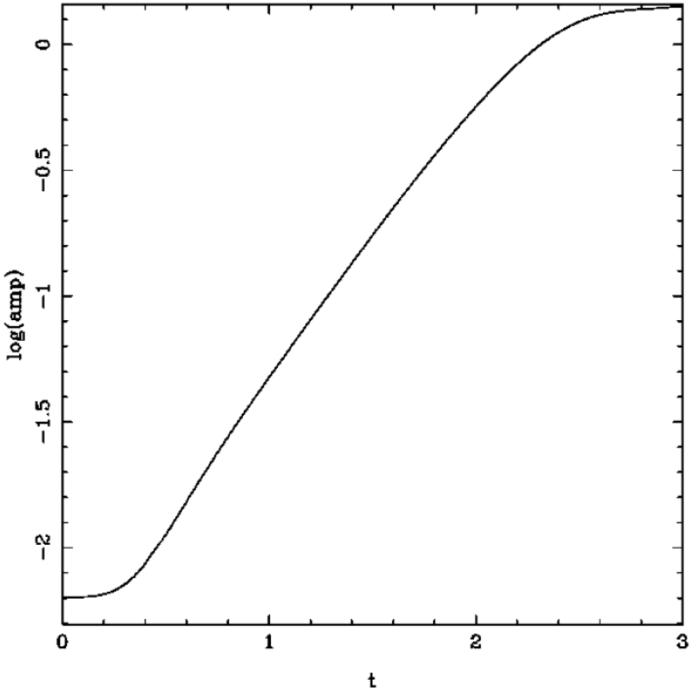
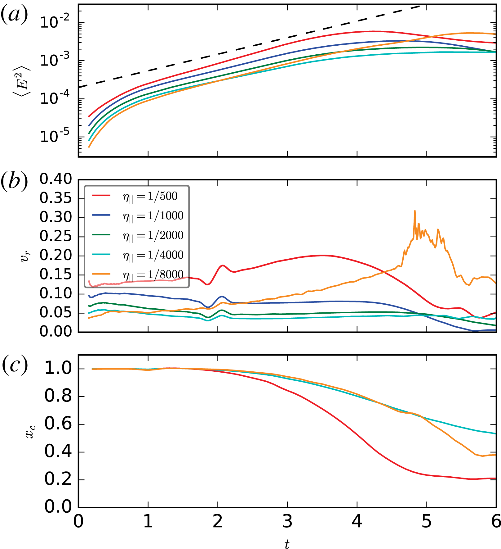
is an amplitude of a perturbations. We find that this leads to the earlier onset of the nonlinear stage of instability depending on the amplitude of perturbations, figure 19.
Electromagnetic energy and perturbation amplitude of force-free simulations as functions of time for a case of initial state with finite amplitude perturbations, chosen to have a large contribution from unstable modes. In comparison with the unstressed system of magnetic islands (figure 7 a), the instability starts to grow immediately.

To find configurations that immediately display a large reconnecting electric field, we turn to the stressed single island case. This is just a cut-out of the multiple island ABC fields, adopting an aspect ratio
 $R\neq 1$
. We choose
 $R=0.9$
as initial perturbation. We choose three different values for the parallel conductivity
 $\unicode[STIX]{x1D705}_{\Vert }\in [500,1000,2000]$
and set the perpendicular component to zero
 $\unicode[STIX]{x1D705}_{\bot }=0$
.
The overall evolution is displayed in figures 20–22.
Time evolution of the out-of-plane field, case
 $\unicode[STIX]{x1D705}_{\Vert }=2000$
, triggered collapse of magnetic islands. The initial X-point collapses and forms a rapidly expanding current-sheet. After
 $t=1$
, the fast evolution is over and the islands oscillate. Times are
 $t\in [0,0.1,0.2,0.3,2,3]$
.

Zoom into the central region showing the quantity
 $1-E^{2}/B^{2}$
, triggered collapse of magnetic islands. At
 $t=0.1$
, two disconnected regions of
 $E\sim B$
exist which rapidly expand.
 $E/B$
in these regions gets smaller as time progresses. Actually, before
 $t=0.1$
,
 $E/B$
reaches values as high as
 $3$
for this case with
 $\unicode[STIX]{x1D705}_{\Vert }=2000$
(see figure 22).

Evolution of critical quantities in the stressed island case for various conductivities. Immediately a region of
 $E>B$
is established. All cases agree in the initial growth rates of
 $v_{r}$
and
 $\langle E^{2}\rangle$
and in the overall time of the evolution. This result is consistent with the initial ideal evolution of the instability.

3.2 Collision-triggered merger of magnetic islands: MHD simulations
Next, we study the role of collisions in triggering magnetic reconnection and dissipation using the framework of resistive force-free electrodynamics (magnetodynamics). In the fluid frame, the structure of colliding flows is that of the unstressed 2-D ABC configuration. In order obtain its structure in the laboratory frame one can simply apply the Lorentz transformation for the electromagnetic field. Hence for the flow moving along the
 $x$
axis to the left with speed
 $v$
, we have
 $$\begin{eqnarray}\displaystyle \left.\begin{array}{@{}c@{}}B_{x}=-\text{sin}(2\unicode[STIX]{x03C0}y/L)B_{0},\\ B_{y}=\unicode[STIX]{x1D6E4}\sin (2\unicode[STIX]{x03C0}\unicode[STIX]{x1D6E4}x/L)B_{0},\\ B_{z}=\unicode[STIX]{x1D6E4}[(\cos (2\unicode[STIX]{x03C0}\unicode[STIX]{x1D6E4}x/L)+\cos (2\unicode[STIX]{x03C0}y/L))]B_{0},\\ E_{x}=0,\\ E_{y}=-v\unicode[STIX]{x1D6E4}[(\cos (2\unicode[STIX]{x03C0}\unicode[STIX]{x1D6E4}x/L)+\cos (2\unicode[STIX]{x03C0}y/L))]B_{0},\\ E_{z}=v\unicode[STIX]{x1D6E4}\sin (2\unicode[STIX]{x03C0}\unicode[STIX]{x1D6E4}x/L)B_{0},\end{array}\right\} & & \displaystyle\end{eqnarray}$$
where
 $\unicode[STIX]{x1D6E4}$
is the Lorentz factor. By replacing
 $v$
with
 $-v$
, we obtain the solution for the flow moving to right with the same speed. To initiate the collision, one can introduce at
 $t=0$
a discontinuity at
 $x=0$
so that the flow is moving to the left for
 $x>0$
and to the right for
 $x<0$
. The corresponding jumps at
 $x=0$
are
 $$\begin{eqnarray}[B_{x}]=[B_{z}]=[E_{x}]=[E_{z}=0],\quad [B_{y}]=2B_{y}^{(r)},\quad [E_{y}]=2E_{y}^{(r)},\end{eqnarray}$$
where index
 $(r)$
refers to the value to the right of the discontinuity. Instead of studying the domain which includes both flows, one can treat
 $x=0$
as a boundary with the boundary conditions described by (3.2) and deal only with the left (or the right) half of the domain. This is exactly what we did in our simulations.
In the simulations, we set
 $B_{0}=1$
,
 $\unicode[STIX]{x1D6E4}=3$
and used the computational domain
 $(0,3L)\times (-L,L)$
, with a uniform grid of
 $600\times 400$
computational cells. The boundary at
 $x=3L$
is treated as an inlet of the flow described by (3.1). Hence the solution at this boundary is given by these equation with
 $x$
replaced by
 $x+vt$
. The magnetic Reynolds number is
 $Re_{m}=10^{3}$
.
Collision-induced merger of magnetic islands. The plots show the distribution of
 $B_{z}$
(a),
 $B\cdot E$
(b) and
 $B_{x}$
(c) at time
 $t=4$
.

Figure 23 illustrates the solution at
 $t=4$
. To the right of
 $x=2$
the flow structure is the same as in the initial solution. In the plot of
 $B_{z}$
(a), one can clearly see the lattice of magnetic islands. It appears compressed along the
 $x$
axis, which is a signature of the relativistic length contraction effect. To the left of
 $x=2$
, the islands rapidly merge and form horizontal stripes of oppositely directed
 $B_{z}$
. The in-plane magnetic field is concentrated in the current sheets separating these stripes.
Shock-induced merger of magnetic islands. (a–d) Show the distribution of the magnetic pressure
 $p_{m}=(B^{2}-E^{2})/2$
at time
 $t=1,2,3$
and 4 (increasing from left to right and from top to bottom).

Collision of uniform flows. (a) The
 $B_{y}$
component of the magnetic field at
 $t=1$
. Both the fast wave and Alvfén waves are easily identified on the plot. (b) The
 $B_{z}$
component of the magnetic field. (c) The magnetic pressure
 $p_{m}=(B^{2}-E^{2})/2$
at the same time. Only the fast wave can be seen on this plot.

Figure 24 shows the time evolution of the flow using the Lorentz-invariant parameter
 $p_{m}=(B^{2}-E^{2})/2$
, which plays the role of magnetic pressure. One can see that the evolution can be described as a wave propagation in the direction away from the plane of collision. Behind this wave the magnetic pressure increases and the wave speed is significantly lower than the speed of light.
The wave properties are very different from those of the basic hyperbolic waves of magnetodynamics. To illustrate this fact, figure 25 shows the solution of the Riemann problem
 $$\begin{eqnarray}\displaystyle \left.\begin{array}{@{}c@{}}\text{Left state:}\quad B=(2,1,2),\quad E=(0,0,-v);\\ \text{Right state:}\quad B=(2,-1,2),\quad E=(0,0,v),\end{array}\right\} & & \displaystyle\end{eqnarray}$$
which describes the collision of two uniform flows. The collision speed
 $v$
is the same as before (
 $\unicode[STIX]{x1D6E4}=3$
). The collision creates both the fast wave (FW) and the Alfvén wave (AW). One can see that, the fast wave propagates with the speed of light and the magnetic pressure is invariant across the AW (Komissarov Reference Komissarov2002).
Comparing the results of the test Riemann problem with the main simulations, we conclude that the main wave is not an AW because the magnetic pressure is not invariant and not FW as its speed is significantly less than the speed of light. In fact, (
 $t=1$
) of figure 24(a) shows a weak linear feature located at
 $x=1$
which can be identified with the FW produced by the collision. A similar, but weaker feature can also be seen in (b) (
 $t=2$
). Presumably, this wave gets scattered by the inhomogeneities of the incoming flow and gradually loses coherence. Other fine arc-like features seen in front of the main wave (e.g. in the region
 $1.2<x<1.7$
) are likely to be fast waves emitted by the turbulence downstream of the main wave.
The main wave, which we will refer to as the dissipation front, seems to start as an Alfvén wave. Immediately downstream of the Alfvén wave, the
 $B_{z}$
component of the magnetic field increases (see figure 25
b), and hence the ABC configuration remains highly squashed along the
 $x$
-axis. However, the flow comes to halt in the
 $x$
direction and the X-points are now highly stressed in the fluid frame.Footnote
8
This leads to their immediate collapse and rapid merger of the ABC islands, as described in § 3.1. The increase of
 $p_{m}$
seems to be a product of magnetic dissipation that follows the merger.
Since the dissipation front is not a well-defined surface of fixed shape, it is rather difficult to measure its speed. However even naked eye inspection of the plots suggest that it monotonically decreases with time with saturation towards the end of the run. Crude measurements based on the position of first features showing strong deviation from the properties of incoming flow give
 $v_{df}\simeq 0.73,0.47,0.45,0.40,0.38$
and 0.37.
To see how the magnetic dissipation can influence the front speed, we analyse the energy and momentum conservation in our problem (This approach is similar to that used by Lyubarsky (Reference Lyubarsky2003).) To simplify the analysis we ignore the complicated electromagnetic structure of flow and assume that the magnetic field is parallel to the front. Denote the front position as
 $x_{df}$
and use indexes 1 and 2 to indicate the flow parameters upstream of the front and downstream of its dissipation zone the front respectively. Since our equations do not include particles pressure and energy, and the dissipated electromagnetic energy simply vanishes this analysis is only relevant for the case of rapid radiative cooling.
Since the flow grounds to halt downstream of the dissipation front, the momentum conservation in the computational box
 $[0,x_{r}]$
 $$\begin{eqnarray}\frac{\text{d}}{\text{d}t}(-v_{1}B_{1}^{2}(x_{b}-x_{df}))=\frac{B_{2}^{2}}{2}-\frac{1}{2}(B_{1}^{2}+v_{1}^{2}B_{1}^{2}),\end{eqnarray}$$
where
 $v_{1}=E_{1}/B_{1}$
. Hence
 $$\begin{eqnarray}B_{1}^{2}v_{df}v_{1}=\frac{B_{2}^{2}}{2}-\frac{1}{2}B_{1}^{2}(1+v_{1}^{2}).\end{eqnarray}$$
Similarly, we obtain the energy conservation law
 $$\begin{eqnarray}\frac{B_{2}^{2}}{2}v_{df}-\frac{1}{2}v_{df}B_{1}^{2}(1+v_{1}^{2})=v_{1}B_{1}^{2}-Q_{d},\end{eqnarray}$$
where
 $Q_{d}$
is the dissipation rate of the front. Solving the last two equation for
 $B_{2}$
and
 $v_{df}$
, we obtain the simple result for the velocity of the shock
 $$\begin{eqnarray}v_{s}^{2}=1-\unicode[STIX]{x1D6FC},\end{eqnarray}$$
where
 $\unicode[STIX]{x1D6FC}=Q_{d}/v_{1}B_{1}^{2}$
is the fraction of the incoming energy flux which is dissipated and lost in the dissipation front, the dissipation efficiency. From this we find that in the absence of dissipation the shock speed equals to the speed of light and thus recover the result for ideal magnetodynamics. In the opposite case of total dissipation, the front speed vanishes, as expected. The final value of
 $v_{s}=0.37$
found in our simulations corresponds to the dissipation efficiency
 $\unicode[STIX]{x1D6FC}=86\,\%$
.
Temporal evolution of the electric energy (a) (in units of the total initial energy) and of the maximum particle Lorentz factor (b) (
 $\unicode[STIX]{x1D6FE}_{\text{max}}$
is defined in (2.3), and it is normalized to the thermal Lorentz factor
 $\unicode[STIX]{x1D6FE}_{th}\simeq 1+(\hat{\unicode[STIX]{x1D6FE}}-1)^{-1}kT/mc^{2}$
), for a suite of five PIC simulations of ABC collapse with fixed
 $kT/mc^{2}=10^{2}$
,
 $\unicode[STIX]{x1D70E}_{in}=42$
and
 $L/r_{L,\text{hot}}=126$
, but different magnitudes of the initial velocity shear (see (3.8)):
 $v_{\text{push}}/c=10^{-1}$
(black),
 $v_{\text{push}}/c=10^{-2}$
(blue),
 $v_{\text{push}}/c=10^{-3}$
(green),
 $v_{\text{push}}/c=10^{-4}$
(yellow) and
 $v_{\text{push}}/c=0$
(red). The dashed black line in (a) shows that the electric energy grows exponentially as
 $\propto \text{exp}\,(4ct/L)$
. The vertical dotted lines mark the time when the electric energy peaks (colours correspond to the five values of
 $v_{\text{push}}/c$
, as described above).

3.3 Driven ABC evolution: PIC simulation
3.3.1 Two-dimensional ABC structures with initial shear
Next we investigate a driven evolution of the ABC structures using PIC simulations. Inspired by the development of the oblique mode described in figure 2, we set-up our system with an initial velocity in the oblique direction, so that two neighbouring chains of ABC islands will shear with respect to each other. More precisely, we set-up an initial velocity profile of the form
 $$\begin{eqnarray}\displaystyle \left.\begin{array}{@{}c@{}}v_{x}=-v_{\text{push}}\cos [\unicode[STIX]{x03C0}(x+y)/L]/\sqrt{2}\\ v_{y}=-v_{x}\\ v_{z}=0\end{array}\right\} & & \displaystyle\end{eqnarray}$$
and we explore the effect of different values of
 $v_{\text{push}}$
.Footnote
9
Figure 26 shows that the evolution of the electric energy ((a), in units of the total initial energy) is remarkably independent of
 $v_{\text{push}}$
, apart from an overall shift in the onset time. In all the cases, the electric energy grows exponentially as
 $\propto \text{exp}\,(4ct/L)$
(compare with the black dashed line) until it peaks at
 ${\sim}10\,\%$
of the total initial energy (the time when the electric energy peaks is indicated with the vertical coloured dotted lines). In parallel, the maximum particle energy
 $\unicode[STIX]{x1D6FE}_{\text{max}}$
grows explosively (figure 26
b), with a temporal profile that is nearly identical in all the cases (once again, apart from an overall time shift). The initial value of the electric energy scales as
 $v_{\text{push}}^{2}$
for large
 $v_{\text{push}}$
(black for
 $v_{\text{push}}/c=10^{-1}$
and blue for
 $v_{\text{push}}/c=10^{-2}$
), just as a consequence of the electric field
 $-\boldsymbol{v}_{\text{push}}\times \boldsymbol{B}/c$
that we initialize. At smaller values of
 $v_{\text{push}}$
, the initial value of the electric energy is independent of
 $v_{\text{push}}$
(green to red curves in a). Here, we are sensitive to the electric field required to build up the particle currents implied by the steady ABC set-up. Overall, the similarity of the different curves in figure 26 (all the way to the undriven case of
 $v_{\text{push}}=0$
, in red) confirms that the oblique ‘shearing’ mode is a natural instability avenue for 2-D ABC structures.
As a consequence, it is not surprising that the particle spectrum measured at the time when the electric energy peaks (as indicated by the vertical coloured lines in figure 26) bears no memory of the driving speed
 $v_{\text{push}}$
. In fact, the five curves in figure 27 nearly overlap.
Particle spectrum at the time when the electric energy peaks, for a suite of five PIC simulations of ABC collapse with fixed
 $kT/mc^{2}=10^{2}$
,
 $\unicode[STIX]{x1D70E}_{in}=42$
and
 $L/r_{L,\text{hot}}=126$
, but different magnitudes of the initial velocity shear (same runs as in figure 26):
 $v_{\text{push}}/c=10^{-1}$
(black),
 $v_{\text{push}}/c=10^{-2}$
(blue),
 $v_{\text{push}}/c=10^{-3}$
(green),
 $v_{\text{push}}/c=10^{-4}$
(yellow) and
 $v_{\text{push}}/c=0$
(red). The main plot shows
 $\unicode[STIX]{x1D6FE}\,\text{d}N/\text{d}\unicode[STIX]{x1D6FE}$
to emphasize the particle content, whereas the inset presents
 $\unicode[STIX]{x1D6FE}^{2}\text{d}N/\text{d}\unicode[STIX]{x1D6FE}$
to highlight the energy census. The dotted black line is a power law
 $\unicode[STIX]{x1D6FE}\,\text{d}N/\text{d}\unicode[STIX]{x1D6FE}\propto \unicode[STIX]{x1D6FE}^{-1}$
, corresponding to equal energy content per decade (which would result in a flat distribution in the inset).

Temporal evolution of the instability of a typical 2-D ABC structure (time is indicated in the grey box of a–f) with an initial stress of
 $\unicode[STIX]{x1D706}=0.94$
(see Paper I for the definition of
 $\unicode[STIX]{x1D706}$
in the context of solitary X-point collapse). The plot presents the 2-D pattern of the out-of-plane field
 $B_{z}$
(in units of
 $B_{0,in}$
) from a PIC simulation with
 $kT/mc^{2}=10^{-4}$
,
 $\unicode[STIX]{x1D70E}_{in}=42$
and
 $L=126\,r_{L,\text{hot}}$
, performed within a domain of size
 $2L\times 2\unicode[STIX]{x1D706}L$
. The system is initially squeezed along the
 $y$
direction. This leads to X-point collapse and formation of current sheets (see the current sheet at
 $x=0$
and
 $y=0.5L$
in b). The resulting reconnection outflows push away neighbouring magnetic structures (the current sheet at
 $x=0$
and
 $y=0.5L$
pushes away the two blue islands at
 $y=0.5L$
and
 $x=\pm 0.5L$
). The system is now squeezed along the
 $x$
direction (c), and it goes unstable on a dynamical time (d), similarly to the case of spontaneous (i.e. unstressed) ABC instability. The subsequent evolution closely resembles the case of spontaneous ABC instability shown in figure 8.

Temporal evolution of various quantities, from a 2-D PIC simulation of ABC instability with
 $kT/mc^{2}=10^{-4}$
,
 $\unicode[STIX]{x1D70E}_{in}=42$
and
 $L=126\,r_{L,\text{hot}}$
and stress parameter
 $\unicode[STIX]{x1D706}=0.94$
, performed within a domain of size
 $2L\times 2\unicode[STIX]{x1D706}L$
(the same run as in figure 28). (a) Fraction of energy in magnetic fields (solid blue), in-plane magnetic fields (dashed blue, with
 $\unicode[STIX]{x1D716}_{B,in}=\unicode[STIX]{x1D716}_{B}/2$
in the initial configuration), electric fields (green) and particles (red; excluding the rest mass energy), in units of the total initial energy. (b) Evolution of the maximum Lorentz factor
 $\unicode[STIX]{x1D6FE}_{\text{max}}$
, as defined in (2.3), relative to the thermal Lorentz factor
 $\unicode[STIX]{x1D6FE}_{th}\simeq 1+(\hat{\unicode[STIX]{x1D6FE}}-1)^{-1}kT/mc^{2}$
, which for our case is
 $\unicode[STIX]{x1D6FE}_{th}\simeq 1$
. The early growth of
 $\unicode[STIX]{x1D6FE}_{\text{max}}$
up to
 $\unicode[STIX]{x1D6FE}_{\text{max}}/\unicode[STIX]{x1D6FE}_{th}\sim 1.5\times 10^{2}$
is due to particle acceleration at the current sheets induced by the initial stress. The subsequent development of the ABC instability at
 $ct/L\simeq 4$
is accompanied by little field dissipation (
 $\unicode[STIX]{x1D716}_{\text{kin}}/\unicode[STIX]{x1D716}_{\text{tot}}(0)\sim 0.1$
) but dramatic particle acceleration, up to
 $\unicode[STIX]{x1D6FE}_{\text{max}}/\unicode[STIX]{x1D6FE}_{th}\sim 10^{3}$
. In (a,b), the vertical dotted black line indicates the time when the electric energy peaks.

3.3.2 Two-dimensional ABC structures with initial stress
We now investigate the evolution of ABC structures in the presence of an initial stress, quantified by the stress parameter
 $\unicode[STIX]{x1D706}$
(see Paper I for the definition of
 $\unicode[STIX]{x1D706}$
in the context of solitary X-point collapse). The unstressed cases discussed so far would correspond to
 $\unicode[STIX]{x1D706}=1$
. The simulation box will be a rectangle with size
 $2L$
along the
 $x$
direction and
 $2\unicode[STIX]{x1D706}L$
along the
 $y$
direction, with periodic boundary conditions.
Figure 28 shows the temporal evolution of the 2-D pattern of the out-of-plane field
 $B_{z}$
(in units of
 $B_{0,in}$
) from a PIC simulation with
 $kT/mc^{2}=10^{-4}$
,
 $\unicode[STIX]{x1D70E}_{in}=42$
and
 $L=126\,r_{L,\text{hot}}$
. The system is initially squeezed along the
 $y$
direction, with a stress parameter of
 $\unicode[STIX]{x1D706}=0.94$
(a). The initial stress leads to X-point collapse and formation of current sheets (see the current sheet at
 $x=0$
and
 $y=0.5L$
in b). This early phase results in a minimal amount of magnetic energy dissipation (see figure 29
a, with the solid blue line indicating the magnetic energy and the red line indicating the particle kinetic energy), but significant particle acceleration. As indicated in figure 29(b), the high-energy cutoff
 $\unicode[STIX]{x1D6FE}_{\text{max}}$
of the particle distribution grows quickly (within one dynamical time) up to
 $\unicode[STIX]{x1D6FE}_{\text{max}}/\unicode[STIX]{x1D6FE}_{th}\sim 1.5\times 10^{2}$
. At this point (
 $ct/L\gtrsim 1$
), the increase in the maximum particle energy stalls. In figure 28, we find that this corresponds to a phase in which the system tends to counteract the initial stress. In particular, the reconnection outflows emanating from the current sheets in figure 28(b) push away neighbouring magnetic structures (the current sheet at
 $x=0$
and
 $y=0.5L$
pushes away the two blue islands at
 $y=0.5L$
and
 $x=\pm 0.5L$
). The system gets squeezed along the
 $x$
direction (c), i.e. the stress is now opposite to the initial stress. Shortly thereafter, the ABC structure goes unstable on a dynamical time scale (d), with a pattern similar to the case of spontaneous (i.e. unstressed) ABC instability. In particular, figure 28(d) shows that in this case the instability proceeds via the ‘parallel’ mode depicted in figure 3 (but other simulations are dominated by the ‘oblique’ mode sketched in figure 2). The subsequent evolution closely resembles the case of spontaneous ABC instability shown in figure 8, with the current sheets stretching up to a length
 ${\sim}L$
and the merger of islands having the same
 $B_{z}$
polarity (figure 28
e), until only two regions remain in the box, with
 $B_{z}$
fields of opposite polarity (figure 28
f).
The second stage of evolution – resembling the spontaneous instability of unstressed ABC structures – leads to a dramatic episode of particle acceleration (see the growth in
 $\unicode[STIX]{x1D6FE}_{\text{max}}$
in figure 29(b) at
 $ct/L\sim 4$
), with the energy spectral cutoff extending beyond
 $\unicode[STIX]{x1D6FE}_{\text{max}}/\unicode[STIX]{x1D6FE}_{th}\sim 10^{3}$
within one dynamical time. This fast increase in
 $\unicode[STIX]{x1D6FE}_{\text{max}}$
is indeed reminiscent of what we had observed in the case of unstressed ABC instability (compare with figure 9
b at
 $ct/L\sim 5$
). In analogy to the case of unstressed ABC structures, the instability leads to dramatic particle acceleration, but only minor energy dissipation (the mean kinetic energy reaches a fraction
 ${\sim}0.1$
of the overall energy budget). Additional dissipation of magnetic energy into particle heat (but without much non-thermal particle acceleration) occurs at later times (
 $ct/L\gtrsim 6$
) during subsequent island mergers, once again imitating the evolution of unstressed ABC instability.
Particle spectrum and synchrotron spectrum from a 2-D PIC simulation of ABC instability with
 $kT/mc^{2}=10^{-4}$
,
 $\unicode[STIX]{x1D70E}_{in}=42$
and
 $L=126\,r_{L,\text{hot}}$
and stress parameter
 $\unicode[STIX]{x1D706}=0.94$
, performed within a domain of size
 $2L\times 2\unicode[STIX]{x1D706}L$
(the same run as in figures 28 and 29). Time is measured in units of
 $L/c$
, see the colour bar at the top. (a) Evolution of the electron energy spectrum normalized to the total number of electrons. At late times, the spectrum approaches a distribution of the form
 $\unicode[STIX]{x1D6FE}\,\text{d}N/\text{d}\unicode[STIX]{x1D6FE}\propto \unicode[STIX]{x1D6FE}^{-1}$
, corresponding to equal energy content in each decade of
 $\unicode[STIX]{x1D6FE}$
(compare with the dotted black line). The inset in (a) shows the electron momentum spectrum along different directions (as indicated in the legend), at the time when the electric energy peaks (as indicated by the dotted black line in figure 29). (b) Evolution of the angle-averaged synchrotron spectrum emitted by electrons. The frequency on the horizontal axis is normalized to
 $\unicode[STIX]{x1D708}_{B,in}=\sqrt{\unicode[STIX]{x1D70E}_{in}}\unicode[STIX]{x1D714}_{p}/2\unicode[STIX]{x03C0}$
. At late times, the synchrotron spectrum approaches
 $\unicode[STIX]{x1D708}L_{\unicode[STIX]{x1D708}}\propto \unicode[STIX]{x1D708}^{1/2}$
(compare with the dotted black line), which just follows from the electron spectrum
 $\unicode[STIX]{x1D6FE}\,\text{d}N/\text{d}\unicode[STIX]{x1D6FE}\propto \unicode[STIX]{x1D6FE}^{-1}$
. The inset in (b) shows the synchrotron spectrum at the time indicated in figure 29 (dotted black line) along different directions (within a solid angle of
 $\unicode[STIX]{x0394}\unicode[STIX]{x1D6FA}/4\unicode[STIX]{x03C0}\sim 3\times 10^{-3}$
), as indicated in the legend in the inset of (a).

The two distinct evolutionary phases – the early stage driven by the initial stress, and the subsequent dynamical ABC collapse resembling the unstressed case – are clearly apparent in the evolution of the particle energy spectrum (figure 30
a) and of the angle-averaged synchrotron emission (figure 30
b). The initial stress drives fast particle acceleration at the resulting current sheets (from black to dark blue in a). Once the stress reverses, as part of the self-consistent evolution of the system (figure 28
b), the particle energy spectrum freezes (see the clustering of the dark blue lines). Correspondingly, the angle-averaged synchrotron spectrum stops evolving (see the clustering of the dark blue lines in b). A second dramatic increase in the particle and emission spectral cutoff (even more dramatic than the initial growth) occurs between
 $ct/L\sim 3$
and
 $ct/L\sim 6$
(dark blue to cyan curves in figure 30), and it directly corresponds to the phase of ABC instability resembling the unstressed case. The particle spectrum quickly extends up to
 $\unicode[STIX]{x1D6FE}_{\text{max}}\sim 10^{3}$
(cyan lines in a), and correspondingly the peak of the
 $\unicode[STIX]{x1D708}L_{\unicode[STIX]{x1D708}}$
emission spectrum shifts up to
 ${\sim}\unicode[STIX]{x1D6FE}_{\text{max}}^{2}\unicode[STIX]{x1D708}_{B,in}\sim 10^{6}\unicode[STIX]{x1D708}_{B,in}$
(cyan lines in b). At times later than
 $c/L\sim 6$
, the evolution proceeds slower, similarly to the case of unstressed ABC instability: the high-energy cutoff in the particle spectrum shifts up by only a factor of three before saturating (green to red curves in a), and the peak frequency of the synchrotron spectrum increases by less than a factor of ten (green to red curves in b). Rather than non-thermal particle acceleration, the late evolution is accompanied by substantial heating of the bulk of the particles, with the peak of the particle spectrum shifting from
 $\unicode[STIX]{x1D6FE}\sim 1$
up to
 $\unicode[STIX]{x1D6FE}\sim 10$
after
 $ct/L\sim 6$
(see also the red line in figure 29(a) at
 $ct/L\gtrsim 6$
, indicating efficient particle heating). Once again, this closely parallels the late time evolution of unstressed ABC instability.
Finally, we point out that the particle distribution at the time when the electric energy peaks (indicated by the vertical dotted line in figure 29) is nearly isotropic, as indicated by the inset in figure 30(a). In turn, this results in quasi-isotropic synchrotron emission (inset in b). We refer to the unstressed case in figure 10 for an explanation of this result, which is peculiar to the ABC geometry employed here.
Temporal evolution of the electric energy (a) (in units of the total initial energy) and of the maximum particle Lorentz factor (b) (
 $\unicode[STIX]{x1D6FE}_{\text{max}}$
is defined in (2.3), and it is normalized to the thermal Lorentz factor
 $\unicode[STIX]{x1D6FE}_{th}\simeq 1+(\hat{\unicode[STIX]{x1D6FE}}-1)^{-1}kT/mc^{2}$
), for a suite of five PIC simulations of ABC collapse with fixed
 $kT/mc^{2}=10^{-4}$
,
 $\unicode[STIX]{x1D70E}_{in}=42$
and
 $L/r_{L,\text{hot}}=126$
, but different magnitudes of the initial stress:
 $\unicode[STIX]{x1D706}=0.78$
(black), 0.87 (blue), 0.94 (green), 0.97 (yellow) and 1 (red; i.e. unstressed). The early phases (until
 $ct/L\sim 3$
) bear memory of the prescribed stress parameter
 $\unicode[STIX]{x1D706}$
, whereas the evolution subsequent to the ABC collapse at
 $ct/L\sim 4$
is remarkably similar for different values of
 $\unicode[STIX]{x1D706}$
. The dashed black line in (a) shows that the electric energy grows exponentially as
 $\propto \exp (4ct/L)$
, during the dynamical phase of the ABC instability. The vertical dotted lines mark the time when the electric energy peaks (colors correspond to the five values of
 $\unicode[STIX]{x1D706}$
, as described above; the black, green and yellow vertical lines overlap).

Particle spectrum at the time when the electric energy peaks, for a suite of five simulations of ABC collapse with fixed
 $kT/mc^{2}=10^{-4}$
,
 $\unicode[STIX]{x1D70E}_{in}=42$
and
 $L/r_{L,\text{hot}}=126$
, but different magnitudes of the initial stress (same runs as in figure 31):
 $\unicode[STIX]{x1D706}=0.78$
(black), 0.87 (blue), 0.94 (green), 0.97 (yellow) and 1 (red; i.e. unstressed). The main plot shows
 $\unicode[STIX]{x1D6FE}\,\text{d}N/\text{d}\unicode[STIX]{x1D6FE}$
to emphasize the particle content, whereas the inset presents
 $\unicode[STIX]{x1D6FE}^{2}\text{d}N/\text{d}\unicode[STIX]{x1D6FE}$
to highlight the energy census. The dotted black line is a power law
 $\unicode[STIX]{x1D6FE}\,\text{d}N/\text{d}\unicode[STIX]{x1D6FE}\propto \unicode[STIX]{x1D6FE}^{-1}$
, corresponding to equal energy content per decade (which would result in a flat distribution in the inset). The particle spectrum at the time when the electric energy peaks has little dependence on the initial stress parameter
 $\unicode[STIX]{x1D706}$
, and it resembles the result of the spontaneous ABC instability (red curve).

We conclude this subsection by investigating the effect of the initial stress, as quantified by the squeezing parameter
 $\unicode[STIX]{x1D706}$
. In figures 31 and 32, we present the results of a suite of five PIC simulations of ABC collapse with fixed
 $kT/mc^{2}=10^{-4}$
,
 $\unicode[STIX]{x1D70E}_{in}=42$
and
 $L/r_{L,\text{hot}}=126$
, but different magnitudes of the initial stress:
 $\unicode[STIX]{x1D706}=0.78$
(black), 0.87 (blue), 0.94 (green), 0.97 (yellow) and 1 (red; i.e. unstressed). In all the cases, the early phase (until
 $ct/L\sim 3$
) bears memory of the prescribed stress parameter
 $\unicode[STIX]{x1D706}$
. In particular, the value of the electric energy at early times increases for decreasing
 $\unicode[STIX]{x1D706}$
(figure 31
a at
 $ct/L\lesssim 3$
), as the initial stress becomes stronger. In parallel, the process of particle acceleration initiated at the stressed X-points leads to a maximum particle energy
 $\unicode[STIX]{x1D6FE}_{\text{max}}$
that reaches higher values for stronger stresses (i.e. smaller
 $\unicode[STIX]{x1D706}$
, see figure 31
b at
 $ct/L\lesssim 3$
). While the early stage is sensitive to the value of the initial stress, the dramatic evolution happening at
 $ct/L\sim 4$
is remarkably similar for all the values of
 $\unicode[STIX]{x1D706}\neq 1$
explored in figure 31 (black to yellow curves). In all the cases, the electric energy grows exponentially as
 $\propto \text{exp}(4ct/L)$
. Both the growth rate and the peak level of the electric energy (
 ${\sim}0.1$
of the total energy) are remarkably insensitive to
 $\unicode[STIX]{x1D706}$
, and they resemble the unstressed case
 $\unicode[STIX]{x1D706}=1$
(red curve in figure 31), aside from a temporal offset of
 ${\sim}2L/c$
. The fast evolution occurring at
 $ct/L\sim 4$
leads to dramatic particle acceleration (figure 31
b), with the high-energy spectral cutoff reaching
 $\unicode[STIX]{x1D6FE}_{\text{max}}\sim 10^{3}$
within a dynamical time, once again imitating the results of the unstressed case, aside from a temporal shift of
 ${\sim}2L/c$
.
As we have just described, the electric energy peaks during the second phase, when the stressed systems evolve in close similarity with the unstressed set-up. In figure 32, we present a comparison of the particle spectra for different
 $\unicode[STIX]{x1D706}$
(as indicated in the legend), measured at the peak time of the electric energy (as indicated by the vertical dotted lines in figure 31). The spectral shape for all the stressed cases is nearly identical, especially if the initial stress is not too strong (i.e. with the only exception of the black line, corresponding to
 $\unicode[STIX]{x1D706}=0.78$
). In addition, the spectral cutoff is in remarkable agreement with the result of the unstressed set-up (red curve in figure 32), confirming that the evolution of the stressed cases closely parallels the spontaneous ABC instability.
We conclude that this set-up – with an initially imposed stress – does not introduce additional advantages in driving the instability of the ABC structure (unlike the shearing set-up described in the previous subsection, which directly leads to ABC collapse). Still, the perturbation imposed onto the system eventually leads to ABC instability, which proceeds in close analogy to the unstressed case. Particle acceleration to the highest energies is not achieved in the initial phase, which still bears memory of the imposed stress, but rather in the quasi-spontaneous ABC collapse at later times. In order to further test this claim, we have performed the following experiment. After the initial evolution (driven by the imposed stress), we artificially reduce the energies of the highest-energy particles (but still keeping them ultra-relativistic, to approximately preserve the electric currents). The subsequent evolution of the high-energy particle spectrum is similar to what we observe when we do not artificially ‘cool’ the particles, which is another confirmation of the fact that the long-term physics is independent from the initial stress.
4 Merging flux tubes carrying zero total current
In §§ 2 and 3 we considered evolution of the unstable configurations – those of the stressed X-point and 2-D ABC configurations (both stressed and unstressed). We found that during the development of instability of the 2-D ABC configurations the particles are efficiently accelerated during the initial dynamical phase of the merger of current-carrying flux tubes (when the evolution is mostly due to the X-point collapse). There are two key feature of the preceding model that are specific to the initial set-up: (i) each flux tube carries non-zero poloidal current; (ii) the initial 2-D ABC configuration is an unstable equilibrium. It is not clear how generic these conditions and how the details of particle acceleration are affected by these specific properties.
In this section we relax these conditions. We investigate a merger of two flux tubes with zero total current. We will study, using relativistic MHD and PIC simulations, the evolution of colliding flux tubes with various internal structure. Importantly, all the cases under investigation have a common property: they carry zero net poloidal current (either completely distributed electric currents as in the case of configurations (4.1) and (4.2) or balanced by the surface current, (4.5)). Thus, two flux tubes are not attracted to each other – at least initially. All the configurations considered have a common property: the current in the core of the flux tube is balanced by the reverse current in the outer parts.
4.1 Force-free simulations
4.1.1 Merger of Lundquist’s magnetic ropes
First we consider Lundquist’s force-free cylinders, surrounded by uniform magnetic field,
 $$\begin{eqnarray}\boldsymbol{B}_{L}(r\leqslant r_{j})=J_{1}(r\unicode[STIX]{x1D6FC})\boldsymbol{e}_{\unicode[STIX]{x1D719}}+J_{0}(r\unicode[STIX]{x1D6FC})\boldsymbol{e}_{z},\end{eqnarray}$$
Here,
 $J_{0},J_{1}$
are Bessel functions of zeroth and first order and the constant
 $\unicode[STIX]{x1D6FC}\simeq 3.8317$
is the first root of
 $J_{0}$
. We chose to terminate this solution at the first zero of
 $J_{1}$
, which we denote as
 $r_{j}$
and hence continue with
 $B_{z}=B_{z}(r_{j})$
and
 $B_{\unicode[STIX]{x1D719}}=0$
for
 $r>r_{j}$
. Thus the total current of the flux tube is zero. As the result, the azimuthal field vanishes at the boundary of the rope, whereas the poloidal one changes sign inside the rope.
We start with the position of two ropes just touching each other and set the centre positions to be
 $\boldsymbol{x}_{c}=(-r_{j},0)$
and
 $\boldsymbol{x}_{c}=(r_{j},0)$
. The evolution is very slow, given the fact that at the contact the reconnecting field vanishes. To speed things up, we ‘push’ the ropes towards each other by imposing a drift velocity. That is, we initialize the electric field
 $$\begin{eqnarray}\boldsymbol{E}=-(1/c)\boldsymbol{v}_{\text{kick}}\times \boldsymbol{B},\end{eqnarray}$$
where
 $\boldsymbol{v}_{\text{kick}}=(\pm v_{\text{kick}},0,0)$
inside the ropes and here we set
 $v_{\text{kick}}=0.1c$
.
The numerical set-up is as follows. We have adopted the force-free algorithm of Komissarov, Barkov & Lyutikov (Reference Komissarov, Barkov and Lyutikov2007) to create a physics module in the publicly available code MPI-AMRVACFootnote
10
(Keppens et al.
Reference Keppens, Meliani, van Marle, Delmont, Vlasis and van der Holst2012; Porth et al.
Reference Porth, Xia, Hendrix, Moschou and Keppens2014). We simulate a 2-D Cartesian domain with
 $x\in [-6,6]$
and
 $y\in [-3,3]$
at a base resolution of
 $128\times 64$
cells. In the following, the scales are given in units of
 $r_{j}$
. During the evolution, we ensure that the Full width at half maximum (FWHM) of the current density in the current sheet is resolved by at least 16 cells via local adaptive mesh refinement of up to eight levels, each increasing the resolution by a factor of two. Boundary conditions are set to ‘periodic’.
The results are illustrated in figure 2, which shows the distribution of
 $B_{z}$
and
 $\unicode[STIX]{x1D712}\equiv 1-E^{2}/B^{2}$
at
 $t=0,2,5,6,9$
. Interestingly, around the time
 $t\approx 5$
, the cores (with
 $B_{z}$
of the same sign) of the flux tubes begin to merge. This leads to zero guide field in the current sheet and increased reconnection rate. The sudden increase in reconnection rate leads to a strong wave being emitted from the current sheet which is also seen in the decrease to
 $\unicode[STIX]{x1D712}\approx 0.7$
in the outer part of the flux tubes, i.e. in figure 33(g,h).
Merging Lundquist flux tubes with initial kick velocity
 $v_{\text{kick}}=0.1c$
and
 $\unicode[STIX]{x1D702}_{\Vert }=1/1000$
. From top to bottom, we show snapshots at
 $t=[0,2,5,6,9]$
where the coordinates are given in units of initial flux-tube radius
 $r_{j}$
and time is measured in units of
 $c/r_{j}$
. (a,c,e,g,i) Shows the magnitude of the out-of-plane component
 $B_{z}$
. (b,d,f,h,j) Shows plots of
 $\unicode[STIX]{x1D712}=1-E^{2}/B^{2}$
indicating that regions with
 $E\sim B$
emerge in the outflow region of the current sheet. Starting from the small kick velocity, the merger rate starts with initial small kick velocity and speeds up until
 $t\sim 5$
. Exemplary field lines are traced and shown as black lines in (b,d,f,h,j).

The influence of the guide field is investigated in figure 34. In the left column of panels, we show cuts of
 $B^{z}$
along the
 $y=0$
plane. As the in-plane magnetic flux reconnects in the current sheet, the out-of-plane component remains and accumulates, leading to a steep profile with magnetic pressure that opposes the inward motion of reconnecting field lines. At
 $t=5.2$
, the guide field changes sign and the reconnection rate spikes rapidly at a value of
 $v_{r}\approx 0.6$
. This is clearly seen in the right column of panels of figure 34. Thereafter, a guide field of the opposite sign builds up and the reconnection rate slows down again. The position of the flux-tube core as quantified by the peak of
 $B^{z}$
evolves for
 $t<r_{j}/c$
according to the prescribed velocity kick (4.2) but then settles for a slower evolution governed by the resistive time scale.
Merging Lundquist flux tubes. Left: cuts along the
 $y=0$
plane, showing the profile of the guide field for various times. Coordinates are given in terms of
 $r_{j}$
and times in units of
 $r_{j}/c$
. At
 $t\simeq 5.2$
, the guide field in the current sheet at
 $x=0$
changes sign which results in a sharp rise in the reconnection rate and accelerated merger of the cores. Right: domain-averaged electric field
 $\langle E^{2}\rangle$
(top) and other quantities of interest (bottom): reconnection rate, measured as drift velocity through
 $x=\pm 0.1$
(red),
 $x$
-coordinate of the core quantified as peak in
 $B^{z}$
(black) and guide field at the origin
 $B^{z}(0,0)$
(blue). When the guide field changes sign, the reconnection rate spikes at
 $v_{r}\simeq 0.6c$
. This equivalent PIC result is discussed in figure 50.

4.2 Modified Lundquist’s magnetic ropes
4.2.1 Description of set-up
For the following analysis, we consider a modified version of Lundquist’s force-free cylinders discussed in the previous § 4.1.1. The toroidal field is the same as given by (4.1), but the vertical field reads
 $$\begin{eqnarray}B_{z}(r\leqslant r_{j})=\sqrt{J_{0}(\unicode[STIX]{x1D6FC}r)^{2}+C}\end{eqnarray}$$
within a flux tube and is set to
 $B_{z}(r_{j})$
in the external medium. As a result, the sign change of the guide field is avoided and only positive values of
 $B_{z}$
are present. The additional constant
 $C$
sets the minimum (positive) vertical magnetic field component. In the following, we always set
 $C=0.01$
.
Merger of 2-D modified Lundquist flux tubes with initial kick velocity
 $v_{\text{kick}}=0.03c$
and
 $\unicode[STIX]{x1D702}_{\Vert }=1000$
. From top to bottom, we show snapshots at
 $t=[6,9,10,11,1214]$
where the coordinates are given in units of initial flux-tube radius
 $r_{j}$
and time is measured in units of
 $c/r_{j}$
. (a,c,e,g,i,k) Shows magnitude of out-of-plane component
 $B_{z}$
. (b,d,f,h,j,l) Shows plots of
 $\unicode[STIX]{x1D712}=1-E^{2}/B^{2}$
indicating that regions with
 $E\sim B$
emerge in the outflow region of the current sheet. Starting from the small kick velocity, the merger rate starts with initial small kick velocity and speeds up until
 $t\sim 9$
. Exemplary field lines are traced and shown as black lines in (b,d,f,h,j,l).

In this section, we will investigate dependence of reconnection rate and electric field magnitude on the kick velocity and magnetic Reynolds number.
Merger of 2-D modified Lundquist flux tubes showing
 $B_{z}$
with varying kick velocity:
 $v_{\text{kick}}=0.01c$
at
 $t=12$
(a),
 $v_{\text{kick}}=0.03c$
at
 $t=9$
(b),
 $v_{\text{kick}}=0.1c$
at
 $t=6$
(c) and
 $v_{\text{kick}}=0.3c$
at
 $t=5$
(d). The snapshot times are chosen to reflect the maximum reconnection rate
 $v_{r}$
, measured as inflow velocity at
 $x=\pm 0.05$
. See text for details.

4.2.2 Overall evolution
As the current vanishes on the surface of the flux tubes, the initial Lorentz force also vanishes and the flux tubes approach each other on the time scale given by the kick velocity. Then a current sheet is formed at the intersection which reconnects in-plane magnetic flux resulting in an engulfing field. This evolution is illustrated in figure 35 for an exemplary run with
 $(v_{\text{kick}},\unicode[STIX]{x1D702}_{\Vert })=(0.03c,10^{-3})$
, showing out-of-plane magnetic field strength
 $B_{z}$
and the previously introduced parameter
 $\unicode[STIX]{x1D712}=1-E^{2}/B^{2}$
. It can be seen that in the outflow region of the current sheet,
 $\unicode[STIX]{x1D712}$
assumes values as small as
 $\unicode[STIX]{x1D712}_{\text{min}}=0.09$
but the distributed region of
 $\unicode[STIX]{x1D712}\approx 0.7$
that is observed for the unmodified Lundquist tubes is absent. After the peak reconnection rate which for the shown parameters is reached at
 $t\simeq 9$
, the system undergoes oscillations between prolate and oblate shape during which the current sheet shrinks. The oscillation frequency corresponds to a light-crossing time across the structure.
4.2.3 Dependence on kick velocity
We now vary the magnitude of the initial perturbation in the interval
 $v_{\text{kick}}\in [0.03c,0.3c]$
. Figure 36 gives an overview of the morphology when the peak reconnection rate is reached. The reconnection rate is measured as inflowing drift velocity at
 $x=\pm 0.05$
and is averaged over a vertical extent of
 $\unicode[STIX]{x0394}y=0.1$
. For the lower three kick velocities, we obtain a very similar morphology when the peak reconnection rate is reached. With
 $v_{\text{kick}}=0.3c$
, the flux tubes rebound, resulting in emission of waves in the ambient medium. As the flux tubes dynamically react to the large perturbation, it is not possible to force a higher reconnection rate by smashing them together with high velocity, they simply bounce off due to the magnetic tension in each flux tube. However, high velocity perturbations of
 $v_{\text{kick}}=0.1c$
and
 $v_{\text{kick}}=0.3c$
lead to the formation of plasmoids which are absent in the cases with small perturbation and this in turn can impact on the reconnection rate.
A more quantitative view is shown in figure 37 illustrating the evolution of the mean electric energy in the domain
 $\langle E^{2}\rangle (t)$
and reconnection rate as previously defined. One can see that all simulations reach a comparable electric field strength in the domain, independent of the initial perturbation. The electric field grows exponentially with comparable growth rate and also the saturation values are only weakly dependent on the initial perturbation. Indeed, comparing highest and lowest kick velocities, we find that
 $\langle E^{2}\rangle _{\text{max}}$
is within a factor of two for a range of
 $30$
in the velocity perturbation.
Merger of 2-D modified Lundquist flux tubes showing the evolution of domain-averaged electric field
 $\langle E^{2}\rangle$
(a) and reconnection rate
 $v_{r}$
(b). We vary the initial driving velocity from
 $v=0.01c$
to
 $v_{}=0.3c$
. See text for discussion.

In the evolution of
 $\langle E^{2}\rangle (t)$
, one can also read off the oscillation period of
 $P\approx 1r_{j}/c$
, most pronounced in the strongly perturbed case. The span of peak reconnection rates is similar to the mean electric field strength with a range from
 $v_{r}=0.2$
down to
 $v_{r}=0.11$
. The reconnection rate saturates at
 ${\sim}0.1c$
for vanishing initial perturbation. When plasmoids are triggered, as for the case
 $v_{\text{kick}}=0.1$
and
 $v_{\text{kick}}=0.3$
, the run of
 $v_{r}$
shows additional substructure leading to secondary peaks as seen e.g. in the green curve on the lower panel.
4.2.4 Scaling with magnetic Reynolds number
We next investigate the scaling of reconnection rate with magnetic Reynolds number while keeping a fixed kick velocity of
 $0.1c$
. As astrophysical Reynolds numbers are typically much larger than what can be achieved numerically, this is an important check for the applicability of the results. For the force-free case, we simply define the Lundquist number
 $$\begin{eqnarray}S=\frac{r_{j}c}{\unicode[STIX]{x1D702}_{\Vert }}\simeq \unicode[STIX]{x1D702}_{\Vert }^{-1}\end{eqnarray}$$
and check the scaling via the resistivity parameter
 $\unicode[STIX]{x1D702}_{\Vert }$
.
Merger of 2-D modified Lundquist flux tubes for different resistivities
 $\unicode[STIX]{x1D702}_{\Vert }$
with initial kick velocity of
 $0.1c$
. Mean squared electric field in the domain (top) and reconnection speed in units of
 $c$
(bottom). Left: Force-free dynamics. The initial evolution depends on the resistivity but comparable values for the reconnection rate of
 $v_{r}\approx 0.15c$
are obtained for all considered Reynolds numbers. Note that in the case
 $\unicode[STIX]{x1D702}_{\Vert }=1/4000$
plasmoids appear at
 $t\simeq 8$
which are not observed in the other runs. Right: Corresponding resistive MHD evolution with
 $\unicode[STIX]{x1D70E}\in [1.7,10]$
and doubled (dashed) and quadrupled (dotted) magnetization. One can see that the force-free result is approached both in the evolution of
 $\langle E^{2}\rangle$
and
 $v_{r}$
.

Figure 38 (left panel), shows the run of the domain-averaged electric field and the reconnection rate as in figure 37. In general, the initial evolution progresses faster when larger resistivities are considered, suggesting a scaling with the resistive time. However, once a significant amount of magnetic flux has reconnected, the electric energy in the domain peaks at values within a factor of
 $1.5$
for a significant range of Reynolds numbers
 $\unicode[STIX]{x1D702}_{\Vert }\in [1/100,1/4000]$
. Very good agreement is found for the peak reconnection rate of
 $v_{r}\simeq 0.15c$
. The
 $\unicode[STIX]{x1D702}_{\Vert }=1/4000$
run developed plasmoids at
 $t\simeq 8$
which were not observed in the other runs.
We have also conducted a range of experiments in resistive relativistic magnetohydrodynamics (RMHD). The set-up is as the force-free configuration described above, however we now choose constant values for density and pressure such that the magnetization in the flux rope has the range
 $\unicode[STIX]{x1D70E}\in [1.7,10]$
and the Alfvén velocity ranges in
 $v_{A}\in [0.8,0.95]$
. The adiabatic index was chosen as
 $\unicode[STIX]{x1D6FE}=4/3$
. Figure 38 (right panel) shows the resulting evolution of electric field and reconnection rate for a variety of resistivity parameter
 $\unicode[STIX]{x1D702}\in [1/250,1/4000]$
. Note that the green curves in the left and right panel correspond to the same resistivity parameter of
 $\unicode[STIX]{x1D702}_{\Vert },\unicode[STIX]{x1D702}=1/1000$
and cyan (left) and red (right) curves both correspond to
 $\unicode[STIX]{x1D702}_{\Vert },\unicode[STIX]{x1D702}=1/4000$
. The initial evolution up to the wave reflection feature at
 $t=2$
is very similar in both realizations. Afterwards the evolution differs: while the reconnection rate in the force-free run with
 $\unicode[STIX]{x1D702}_{\Vert }=1/4000$
increases to reach a peak of
 $v_{r}\simeq 0.15c$
at
 $t\simeq 9$
,
 $v_{r}$
remains approximately constant in the corresponding RMHD run. In contrast to the force-free scenario, the RMHD runs did not feature any plasmoids at the Reynolds numbers considered here. Better agreement is found for
 $\unicode[STIX]{x1D702}_{\Vert },\unicode[STIX]{x1D702}=1/1000$
(green curves in both panels). Here, the force-free reconnection rate reaches its peak value of
 $v_{r}\simeq 0.14$
at
 $t\simeq 6$
and the RMHD peaks at
 $t\simeq 7$
with
 $v_{r}\simeq 0.07c$
. Increasing the magnetization improves the match between both cases: In the green dashed (dotted) curve, we have doubled (quadrupled) the magnetization by lowering plasma density and pressure in the SRMHD runs at
 $\unicode[STIX]{x1D702}=1/1000$
. One can see that the evolution speeds up and higher reconnection rates are achieved: For the highest magnetization run, we reach the peak reconnection rate of
 $\simeq 0.1c$
and the peak is reached already at
 $t\simeq 6.2$
very similar to the corresponding force-free run which peaked at
 $t\simeq 6$
with
 $v_{r}\simeq 0.13c$
. This indicates that the RMHD model indeed approaches the force-free limit for increasing magnetization.
4.3 Core-envelope magnetic ropes
4.3.1 Description of set-up
We now adopt a set-up where the current does no return volumetrically within the flux tube, but returns as a current sheet on the surface. The solution is based on the ‘core-envelope’ solution of Komissarov (Reference Komissarov1999), with the gas pressure replaced by the pressure of the poloidal field. Specifically, the profiles read
 $$\begin{eqnarray}\displaystyle & \displaystyle B^{\unicode[STIX]{x1D719}}(r)=\left\{\begin{array}{@{}ll@{}}B_{m}(r/r_{m});\quad & r<r_{m}\\ B_{m}(r_{m}/r);\quad & r_{m}<r<r_{j}\\ 0;\quad & r>r_{j},\end{array}\right. & \displaystyle\end{eqnarray}$$
 $$\begin{eqnarray}\displaystyle & \displaystyle B_{z}^{2}(r)/2=\left\{\begin{array}{@{}ll@{}}p_{0}\left[\unicode[STIX]{x1D6FC}+\displaystyle \frac{2}{\unicode[STIX]{x1D6FD}_{m}}(1-(r/r_{m})^{2})\right];\quad & r<r_{m}\\ \unicode[STIX]{x1D6FC}p_{0};\quad & r_{m}<r<r_{j}\\ p_{0};\quad & r>r_{j},\end{array}\right. & \displaystyle\end{eqnarray}$$
where
 $$\begin{eqnarray}\unicode[STIX]{x1D6FD}_{m}=\frac{2p_{0}}{B_{m}^{2}},\qquad \unicode[STIX]{x1D6FC}=1-(1/\unicode[STIX]{x1D6FD}_{m})(r_{m}/r_{j})^{2},\end{eqnarray}$$
 $r_{j}$
is the outer radius of the rope and
 $r_{m}$
is the radius of its core. In the simulations,
 $r_{m}=0.5$
,
 $B_{m}=1$
,
 $\unicode[STIX]{x1D6FC}=0.2$
and the coordinates are scaled to
 $r_{j}=1$
. As in the previous cases, two identical current tubes are centred at
 $(x,y)=(-1,0)$
and
 $(x,y)=(1,0)$
. They are at rest and barely touch each other at
 $(x,y)=(0,0)$
. In this scenario, since the current closes discontinuously at the surface of the flux tubes, the Lorentz force acting on the outer field lines is non-vanishing. Thus we can dispense with the initial perturbation and always set
 $v_{\text{kick}}=0$
.
4.3.2 Overall evolution
The overall evolution is characterized as follows: Immediately, a current sheet forms at the point (0, 0) and two Y-points get expelled in vertical direction with initial speed of
 $c$
. The expansion of the Y-points is thereafter slowed down by the accumulating pressure of
 $B^{z}$
in the ambient medium. Snapshots of
 $B^{z}$
for the case
 $\unicode[STIX]{x1D702}_{\Vert }=1/500$
are shown in figure 39. The stage of most rapid evolution of the cores is at
 $t\simeq 4$
. At this time, the morphology is comparable to the modified Lundquist ropes, i.e. figure 36.
We quantify the evolution of Y-point
 $(0,y_{yp})$
via the peak in
 $E^{x}$
along the
 $x=0$
line and the core location
 $(x_{c},0)$
as peak of
 $B^{z}$
along the
 $y=0$
line. The data are shown in figure 40(a). One can see the Y-point slowing down from its initial very fast motion. Gradually, the cores accelerate their approach, reaching a maximal velocity at
 $t\simeq 4$
. The evolution stalls as the guide field at
 $(0,0)$
reaches its maximum and magnetic pressure in the current sheet balances the tension of the encompassing field.
Merger of 2-D core-envelope flux tubes with
 $\unicode[STIX]{x1D702}_{\Vert }=500$
. We show snapshots showing
 $B^{z}$
at
 $t=[1,2,3,4,5]$
as indicated in (a–f), where the coordinates are given in units of initial flux-tube radius
 $r_{j}$
and time is measured in units of
 $c/r_{j}$
. This figure is to be compared to the PIC results as shown in figure 52.

Merger of 2-D core-envelope flux tubes with
 $\unicode[STIX]{x1D702}_{\Vert }=500$
. (a) Position of the upper Y-Point (solid red) quantified as peak of
 $E^{x}$
on the
 $x=0$
line and right core position (blue dashed) obtained from the peak of
 $B^{z}$
on the
 $x=0$
line. (b) Reconnection rate, measured as drift velocity through
 $x=\pm 0.1$
(solid red) and guide field at the origin
 $B^{z}(0,0)$
(blue dashed). This figure can be compared to the PIC results shown in figure 53.

4.3.3 Scaling with magnetic Reynolds number
As for the modified Lundquist ropes, § 4.2.4, we investigate the dependence of the dynamics with magnetic Reynolds number by varying the resistivity parameter. An overview of relevant quantities is given in figure 41 for the range
 $\unicode[STIX]{x1D702}_{\Vert }\in [1/500,1/8000]$
. After the onset time of
 ${\approx}r_{j}/c$
, all runs enter into a phase where the electric energy grows according to
 $\propto \exp (tc/r_{j})$
. As expected, the electric energy decreases when the conductivity is increased. Between
 $t\simeq 4$
and
 $t\simeq 5$
, the growth of the electric energy saturates and the evolution slows down. In general, we observe two regimes: Up to
 $\unicode[STIX]{x1D702}_{\Vert }=1/4000$
, the reconnection rate decreases with increasing conductivity, as would be expected in a Sweet–Parker scaling. In this regime, also the motion of the cores slows down when
 $\unicode[STIX]{x1D702}_{\Vert }$
is decreased. Whereas the most rapid motion for
 $\unicode[STIX]{x1D702}_{\Vert }=1/500$
was found at
 $t\simeq 4$
, for
 $\unicode[STIX]{x1D702}_{\Vert }=1/4000$
it is delayed to
 $t\simeq 5$
(cf. figure 41
c).
The case with the highest conductivity,
 $\unicode[STIX]{x1D702}_{\Vert }=1/8000$
breaks the trend of the low conductivity cases. Here, the reconnection rate increases continuously up to
 $t\simeq 4.5$
at which point it rapidly flares to a large value of
 $v_{r}\simeq 0.25c$
where it remains for somewhat less than
 $r_{j}/c$
. Also the slowing of the core motion is halted at
 $\unicode[STIX]{x1D702}_{\Vert }=1/8000$
: Up to
 $t\simeq 5$
, the core position lines up well with the case
 $\unicode[STIX]{x1D702}_{\Vert }=1/4000$
. Just after the flare, the flux-tube merger is accelerated as evidenced by the rapid decline of
 $x_{c}$
.
Merger of 2-D core-envelope flux tubes for different resistivities
 $\unicode[STIX]{x1D702}_{\Vert }\in [1/500,1/8000]$
. (a) Domain-averaged electric field strength
 $\langle E^{2}\rangle$
. After one light-crossing time we observe a growth according to
 $\propto \exp (tc/r_{j})$
indicated as black dashed line. (b) Reconnection rate, measured as drift velocity through
 $x=\pm 0.1$
. The dynamical evolution for
 $\unicode[STIX]{x1D702}_{\Vert }=1/8000$
is very different from the cases
 $\unicode[STIX]{x1D702}_{\Vert }=1/1000,1/2000,1/4000$
. In those cases, one large plasmoid would form and remain stationary in the current sheet until very late times (
 $t>6$
). In the lowest resistivity case however, many small plasmoids are created which expel flux continuously to both sides. Thus the magnetic tension surrounding the structure grows more rapidly, leading to the explosive increase of reconnection at
 $t\simeq 4.5$
. (c) Core position for the three selected cases
 $\unicode[STIX]{x1D702}_{\Vert }=1/500,1/4000,1/8000$
. In the regime
 $\unicode[STIX]{x1D702}_{\Vert }\in [1/500,1/4000]$
, the merging of the cores slows down as electric conductivity increases. For
 $\unicode[STIX]{x1D702}_{\Vert }=1/8000$
however, this trend is halted and reversed as the motion of the cores actually speeds up after the peak in reconnection rate at
 $t\simeq 5$
. This figure can be compared to the PIC results shown in figure 57.

It is interesting to ask why the dynamics changed so dramatically for the case
 $\unicode[STIX]{x1D702}_{\Vert }=1/8000$
. In figure 42, we show snapshots of
 $\unicode[STIX]{x1D712}=1-E^{2}/B^{2}$
at the time
 $t=5$
for the two highest conductivity cases. At this point, in the lower conductivity case, a single large central plasmoid has formed that remains in the current sheet for the entire evolution. This qualitative picture also holds for the cases
 $\unicode[STIX]{x1D702}_{\Vert }=1/1000,1/2000$
. Flux that accumulates in the central plasmoid does not get expelled from the current sheet and so does not add to the magnetic tension which pushes the ropes together. Furthermore, the single island opposes the merger via its magnetic pressure of the accumulated
 $B^{z}$
. For the case
 $\unicode[STIX]{x1D702}_{\Vert }=1/8000$
, the large-scale plasmoid does not form, instead smaller plasmoids are expelled symmetrically in both directions. The expelled flux continues to contribute to the large scale stresses and the merger of the islands is accelerated further which is reflected also in the continued exponential rise of the electric energy shown in figure 41. As in the case of the Lundquist and modified Lundquist flux tubes and as required for rapid particle acceleration, macroscopic regions of
 $E>B$
are found also in this configuration in the outflow regions of the current sheet, illustrated in figure 42.
Merger of 2-D core-envelope flux tubes. Comparison of
 $\unicode[STIX]{x1D712}=1-E^{2}/B^{2}$
in the central region for the two highest conductivity cases at the time of the reconnection flare at
 $t=5$
:
 $\unicode[STIX]{x1D702}_{\Vert }=1/4000$
(a) and
 $\unicode[STIX]{x1D702}_{\Vert }=1/8000$
(b). One can clearly see the different qualitative behaviour: in the former case, a single large plasmoid grows in the centre of the current sheet, in the latter case, instead small-scale plasmoids are expelled in both directions. At this time, there are also clear differences in the position of the Y-point: in the high conductivity case, the Y-point is notably further out as the evolution has progressed faster. As the evolution progresses, a large connected charge-starved area develops as seen in (c) for
 $\unicode[STIX]{x1D702}_{\Vert }=1/8000$
at
 $t=5.5r_{j}/c$
.

In conclusion, our force-free experiments of coalescing flux tubes show that large-scale stresses can lead to high reconnection rates in the range of
 $0.1c{-}0.3c$
, independent of the magnetic Reynolds number. The dynamics is highly nonlinear and depends on the details of the reconnection in the current sheet: when a single large plasmoid is formed in the current sheet, rapid instability can be avoided. This was the case in the three intermediate resistivity cases for the core-envelope configuration considered here. Also the original Lundquist tubes showed a rapid reconnection flare of
 $v_{r}\simeq 0.6c$
. The reason is the sign change of the
 $B^{z}$
component, leading to vanishing guide field and a missing restoring force in the current sheet. As guide field with opposite polarity builds up in the current sheet thereafter, the fast reconnection is quickly stalled.
4.4 PIC simulations of 2-D flux-tube mergers: simulation set-up
We study the evolution of 2-D flux tubes with PIC simulations, employing the electromagnetic PIC code TRISTAN-MP (Buneman Reference Buneman1993; Spitkovsky Reference Spitkovsky, Bulik, Rudak and Madejski2005). We analyse two possible field configurations: (i) Lundquist magnetic ropes (see (4.1)), containing zero total current (so, the azimuthal magnetic field vanishes at the boundaries of the rope); (ii) core-envelope ropes (see (4.5) and (4.6)) this configuration has non-zero total volumetric current, which is cancelled by the surface current.
Our computational domain is a rectangle in the
 $x{-}y$
plane, with periodic boundary conditions in both directions. The simulation box is initialized with a uniform density of electron–positron plasma at rest and with the magnetic field appropriate for the Lundquist or core-envelope configuration. Since the azimuthal magnetic field vanishes at the boundaries of the Lundquist ropes, the evolution is very slow. Actually, we do not see any sign of evolution up to the final time
 ${\sim}20\,c/\,r_{j}$
of our simulation of undriven Lundquist ropes. For this reason, we push by hand the two ropes toward each other, with a prescribed
 $v_{\text{push}}$
whose effects will be investigated below. It follows that inside the ropes we start with the magnetic field in (4.1) and with the electric field
 $\boldsymbol{E}=-\boldsymbol{v}_{\text{push}}\times \boldsymbol{B}/c$
, whereas the electric field is initially zero outside the ropes.
The azimuthal magnetic field does not vanish at the boundaries of the core-envelope ropes, and the system evolves self-consistently (so, we do not need to drive the system by hand). Here, both the azimuthal field and the poloidal field are discontinuous at the boundary of the ropes. A particle current would be needed to sustain the curl of the field. In our set-up, the computational particles are initialized at rest, but such electric current gets self-consistently built up within a few time steps. To facilitate comparison with the force-free results, our core-envelope configuration has
 $r_{m}/\,r_{j}=0.5$
and
 $\unicode[STIX]{x1D6FC}=0.2$
, the same values as in the force-free simulation of figure 39.
For our fiducial runs, the spatial resolution is such that the plasma skin depth
 $\,c/\unicode[STIX]{x1D714}_{p}$
is resolved with 2.5 cells, but we have verified that our results are the same up to a resolution of
 $\,c/\unicode[STIX]{x1D714}_{p}=10$
cells. We only investigate the case of a cold background plasma, with initial thermal dispersion
 $kT/mc^{2}=10^{-4}$
.Footnote
11
Each cell is initialized with two positrons and two electrons, but we have checked that our results are the same when using up to 64 particles per cell. In order to reduce noise in the simulation, we filter the electric current deposited onto the grid by the particles, mimicking the effect of a larger number of particles per cell (Spitkovsky Reference Spitkovsky, Bulik, Rudak and Madejski2005; Belyaev Reference Belyaev2015).
Our unit of length is the radius
 $\,r_{j}$
of the flux ropes, and time is measured in units of
 $\,r_{j}/c$
. Our domain is typically a large rectangle of size
 $10\,r_{j}$
along
 $x$
(i.e. along the direction connecting the centres of the two ropes) and of size
 $6\,r_{j}$
along
 $y$
(but we have tested that a smaller domain with
 $5\,r_{j}\times 3\,r_{j}$
gives the same results). A large domain is needed to minimize the effect of the boundary conditions on the evolution of the system.
We explore the dependence of our results on the flow magnetization. We identify our runs via the mean value
 $\unicode[STIX]{x1D70E}_{in}$
of the magnetization measured within the flux ropes using the initial in-plane fields (so, excluding the
 $B_{z}$
field). As we argue below, it is the dissipation of the in-plane fields that primarily drives efficient heating and particle acceleration. In addition, this choice allows for a direct comparison of our results between the two configurations (Lundquist and core envelope) and with the ABC structures of § 2.4. The mean in-plane field corresponding to
 $\unicode[STIX]{x1D70E}_{in}$
shall be called
 $B_{0,in}$
, and it will be our unit of measure of the electromagnetic fields. We will explore a wide range of magnetizations, from
 $\unicode[STIX]{x1D70E}_{in}=3$
up to
 $\unicode[STIX]{x1D70E}_{in}=170$
.
It will be convenient to compare the radius
 $\,r_{j}$
of the ropes to the characteristic Larmor radius
 $r_{L,\text{hot}}=\sqrt{\unicode[STIX]{x1D70E}_{in}}\,c/\unicode[STIX]{x1D714}_{p}$
of the high-energy particles heated/accelerated by reconnection (rather than to the skin depth
 $\,c/\unicode[STIX]{x1D714}_{p}$
). We will explore a wide range of
 $\,r_{j}/r_{L,\text{hot}}$
, from
 $\,r_{j}/r_{L,\text{hot}}=31$
up to
 $245$
. We will demonstrate that the two most fundamental parameters that characterize the system are the magnetization
 $\unicode[STIX]{x1D70E}_{in}$
and the ratio
 $\,r_{j}/r_{L,\text{hot}}$
.
Temporal evolution of 2-D Lundquist ropes (time is measured in
 $c/\,r_{j}$
and indicated in the grey box of each panel, increasing from top to bottom). The plot presents the 2-D pattern of the out-of-plane field
 $B_{z}$
(a,c,e,g,i,k; in units of
 $B_{0,in}$
) and of the in-plane magnetic energy fraction
 $\unicode[STIX]{x1D716}_{B,in}=(B_{x}^{2}+B_{y}^{2})/8\unicode[STIX]{x03C0}nmc^{2}$
(b,d,f,h,j,l; with superimposed magnetic field lines), from a PIC simulation with
 $kT/mc^{2}=10^{-4}$
,
 $\unicode[STIX]{x1D70E}_{in}=43$
and
 $\,r_{j}=61\,r_{L,\text{hot}}$
, performed within a rectangular domain of size
 $10\,r_{j}\times 6\,r_{j}$
(but we only show a small region around the centre). The evolution is driven with a velocity
 $v_{\text{push}}/c=0.1$
. Reconnection at the interface between the two flux ropes (i.e. around
 $x=y=0$
) creates an envelope of field lines engulfing the two islands, whose tension force causes them to merge on a dynamical time. This figure should be compared with the force-free result in figure 33 (even though
 $v_{\text{push}}/c=0.3$
in that case).

Temporal evolution of various quantities, from a 2-D PIC simulation of Lundquist ropes with
 $kT/mc^{2}=10^{-4}$
,
 $\unicode[STIX]{x1D70E}_{in}=43$
and
 $\,r_{j}=61\,r_{L,\text{hot}}$
(the same as in figure 43), performed within a rectangular domain of size
 $5\,r_{j}\times 3\,r_{j}$
. The evolution is driven with a velocity
 $v_{\text{push}}/c=0.1$
. (a) Fraction of energy in magnetic fields (solid blue), in-plane magnetic fields (dashed blue), electric fields (green) and particles (red; excluding the rest mass energy), in units of the total initial energy. (b) Reconnection rate
 $v_{\text{rec}}/c$
(red), defined as the inflow speed along the
 $x$
direction averaged over a square of side equal to
 $\,r_{j}/2$
centred at
 $x=y=0$
; and location
 $x_{c}$
of the core of the rightmost flux rope (black), in units of
 $\,r_{j}$
. (c) Evolution of the maximum Lorentz factor
 $\unicode[STIX]{x1D6FE}_{\text{max}}$
, as defined in (2.3), relative to the thermal Lorentz factor
 $\unicode[STIX]{x1D6FE}_{th}\simeq 1+(\hat{\unicode[STIX]{x1D6FE}}-1)^{-1}kT/mc^{2}$
, which for our case is
 $\unicode[STIX]{x1D6FE}_{th}\simeq 1$
. In response to the initial push,
 $\unicode[STIX]{x1D6FE}_{\text{max}}$
increases at
 $ct/\,r_{j}\sim 2$
up to
 $\unicode[STIX]{x1D6FE}_{\text{max}}/\unicode[STIX]{x1D6FE}_{th}\sim 40$
, before stalling. At this stage, the cores of the two islands have not significantly moved (black line in b). At
 $ct/\,r_{j}\sim 5$
, the tension force of the common envelope of field lines starts pushing the two islands toward each other (and the
 $x_{c}$
location of the rightmost rope decreases, see (b)), resulting in a merger event occurring on a dynamical time scale. During the merger (at
 $ct/\,r_{j}\sim 6$
), the reconnection rate peaks (red line in (b)), a fraction of the in-plane magnetic energy is transferred to the plasma (compare dashed blue and solid red lines in (a)), and particles are quickly accelerated up to
 $\unicode[STIX]{x1D6FE}_{\text{max}}/\unicode[STIX]{x1D6FE}_{th}\sim 10^{3}$
(c). In all the panels, the vertical dotted black line indicates the time when the electric energy peaks, shortly after the most violent phase of the merger event.

4.5 PIC simulations of 2-D flux-tube mergers: Lundquist ropes
The temporal evolution of the merger of two Lundquist ropes is shown in figure 43. The plot presents the 2-D pattern of the out-of-plane field
 $B_{z}$
((a,c,e,g,i,k); in units of
 $B_{0,in}$
) and of the in-plane magnetic energy fraction
 $\unicode[STIX]{x1D716}_{B,in}=(B_{x}^{2}+B_{y}^{2})/8\unicode[STIX]{x03C0}nmc^{2}$
((b,d,f,h,j,l); with superimposed magnetic field lines), from a PIC simulation with
 $kT/mc^{2}=10^{-4}$
,
 $\unicode[STIX]{x1D70E}_{in}=43$
and
 $\,r_{j}=61\,r_{L,\text{hot}}$
. The magnetic ropes are initially driven toward each other with a speed
 $v_{\text{push}}/c=0.1$
(below, we study the dependence on the driving speed). Time is measured in units of
 $\,r_{j}/c$
and indicated in the grey boxes within each panel. The figure should be compared with the force-free result in figure 33 (even though
 $v_{\text{push}}/c=0.3$
in that case).
As the two magnetic ropes slowly approach, driven by the initial velocity push (compare (a,b) and (c,d) in figure 43), reconnection is triggered in the plane
 $x=0$
, as indicated by the formation and subsequent ejection of small-scale plasmoids ((e,f) and (g,h) in figure 43). So far (i.e. until
 $ct/\,r_{j}\sim 4.5$
), the cores of the two islands have not significantly moved (black line in figure 44
b, indicating the
 $x_{c}$
location of the centre of the rightmost island), the reconnection speed is quite small (red line in figure 44
b) and no significant energy exchange has occurred from the fields to the particles (compare the in-plane magnetic energy, shown by the dashed blue line in figure 44(a), with the particle kinetic energy, indicated with the red line).Footnote
12
The only significant evolution before
 $ct/\,r_{j}\sim 4.5$
is the reconnection-driven increase in the maximum particle Lorentz factor up to
 $\unicode[STIX]{x1D6FE}_{\text{max}}/\unicode[STIX]{x1D6FE}_{th}\sim 40$
occurring at
 $ct/\,r_{j}\sim 2.5$
(see the black line in figure 44
c).
As a result of reconnection, an increasing number of field lines, that initially closed around one of the ropes, are now engulfing both magnetic islands. Their tension force causes the two ropes to approach and merge on a quick (dynamical) time scale, starting at
 $ct/\,r_{j}\sim 4.5$
and ending at
 $ct/\,r_{j}\sim 7.5$
(see that the distance of the rightmost island from the centre rapidly decreases, as indicated by the black line in figure 44
b). The tension force drives the particles in the flux ropes toward the centre, with a fast reconnection speed peaking at
 $v_{\text{rec}}/c\sim 0.3$
(red line in figure 44
b).Footnote
13
The reconnection layer at
 $x=0$
stretches up to a length of
 ${\sim}2\,r_{j}$
, it becomes unstable to the secondary tearing mode (Uzdensky et al.
Reference Uzdensky, Loureiro and Schekochihin2010), and secondary plasmoids are formed (e.g. see the plasmoid at
 $(x,y)\sim (0,0)$
at
 $ct/\,r_{j}=6$
). Below, we demonstrate that the formation of secondary plasmoids is primarily controlled by the ratio
 $\,r_{j}/r_{L,\text{hot}}$
. In the central current sheet, it is primarily the in-plane field that gets dissipated (compare the dashed and solid blue lines in figure 44
a), driving an increase in the electric energy (green) and in the particle kinetic energy (red).Footnote
14
In this phase of evolution, the fraction of initial energy released to the particles is small (
 $\unicode[STIX]{x1D716}_{\text{kin}}/\unicode[STIX]{x1D716}_{\text{tot}}(0)\sim 0.1$
), but the particles advected into the central X-point experience a dramatic episode of acceleration. As shown in figure 44(c), the cutoff Lorentz factor
 $\unicode[STIX]{x1D6FE}_{\text{max}}$
of the particle spectrum presents a dramatic evolution, increasing up to
 $\unicode[STIX]{x1D6FE}_{\text{max}}/\unicode[STIX]{x1D6FE}_{th}\sim 10^{3}$
within a couple of dynamical times. It is this phase of extremely fast particle acceleration that we associate with the generation of the Crab flares.
Particle energy spectrum and synchrotron spectrum from a 2-D PIC simulation of Lundquist ropes with
 $kT/mc^{2}=10^{-4}$
,
 $\unicode[STIX]{x1D70E}_{in}=43$
and
 $\,r_{j}=61\,r_{L,\text{hot}}$
(the same as in figures 43 and 44), performed within a domain of size
 $10\,r_{j}\times 6\,r_{j}$
. The evolution is driven with a velocity
 $v_{\text{push}}/c=0.1$
. Time is measured in units of
 $\,r_{j}/c$
, see the colour bar at the top. (a) Evolution of the electron energy spectrum normalized to the total number of electrons. At late times, the high-energy spectrum approaches a hard distribution
 $\unicode[STIX]{x1D6FE}\,\text{d}N/\text{d}\unicode[STIX]{x1D6FE}\propto \text{const.}$
(for comparison, the dotted black line shows the case
 $\unicode[STIX]{x1D6FE}\,\text{d}N/\text{d}\unicode[STIX]{x1D6FE}\propto \unicode[STIX]{x1D6FE}^{-1}$
corresponding to equal energy content in each decade of
 $\unicode[STIX]{x1D6FE}$
). (b) Evolution of the angle-averaged synchrotron spectrum emitted by electrons. The frequency on the horizontal axis is in units of
 $\unicode[STIX]{x1D708}_{B,in}=\sqrt{\unicode[STIX]{x1D70E}_{in}}\unicode[STIX]{x1D714}_{p}/2\unicode[STIX]{x03C0}$
. At late times, the synchrotron spectrum approaches a power law with
 $\unicode[STIX]{x1D708}L_{\unicode[STIX]{x1D708}}\propto \unicode[STIX]{x1D708}$
, which just follows from the fact that the electron spectrum at high energies is close to
 $\unicode[STIX]{x1D6FE}\,\text{d}N/\text{d}\unicode[STIX]{x1D6FE}\propto \text{const}$
. This is harder than the dotted line, which indicates the slope
 $\unicode[STIX]{x1D708}L_{\unicode[STIX]{x1D708}}\propto \unicode[STIX]{x1D708}^{1/2}$
resulting from an electron spectrum
 $\unicode[STIX]{x1D6FE}\,\text{d}N/\text{d}\unicode[STIX]{x1D6FE}\propto \unicode[STIX]{x1D6FE}^{-1}$
.

Particle momentum spectrum and anisotropy of the synchrotron emission from a 2-D PIC simulation of Lundquist ropes with
 $kT/mc^{2}=10^{-4}$
,
 $\unicode[STIX]{x1D70E}_{in}=43$
and
 $\,r_{j}=61\,r_{L,\text{hot}}$
(the same as in figures 43–45), performed within a domain of size
 $10\,r_{j}\times 6\,r_{j}$
. The evolution is driven with a velocity
 $v_{\text{push}}/c=0.1$
. (a) Electron momentum spectrum along different directions (as indicated in the legend), at the time when the electric energy peaks (as indicated by the vertical dotted black line in figure 44). The highest-energy electrons are beamed along the direction
 $y$
of the reconnection outflow (blue lines) and along the direction
 $+z$
of the accelerating electric field (red solid line; positrons will be beamed along
 $-z$
, due to the opposite charge). The inset shows the 1-D profile along
 $y$
of the bulk four-velocity in the outflow direction (i.e. along
 $y$
), measured at
 $x=0$
. (b) Synchrotron spectrum at the time indicated in figure 44 (vertical dotted black line) along different directions (within a solid angle of
 $\unicode[STIX]{x0394}\unicode[STIX]{x1D6FA}/4\unicode[STIX]{x03C0}\sim 3\times 10^{-3}$
), as indicated in the legend. The resulting anisotropy of the synchrotron emission is consistent with the particle anisotropy illustrated in (a).

The two distinct evolutionary phases – the early stage driven by the initial velocity push, and the subsequent dynamical merger driven by large-scale electromagnetic stresses – are clearly apparent in the evolution of the particle energy spectrum (figure 45
a) and of the angle-averaged synchrotron emission (figure 45
b). The initial velocity push drives reconnection in the central current sheet, which leads to fast particle acceleration (from dark blue to cyan in a). This is only a transient event, and the particle energy spectrum then freezes (see the clustering of the cyan lines, and compare with the phase at
 $2.5\lesssim ct/\,r_{j}\lesssim 4$
in figure 44
c). Correspondingly, the angle-averaged synchrotron spectrum stops evolving (see the clustering of the cyan lines in c). A second dramatic increase in the particle and emission spectral cutoff (even more dramatic than the initial growth) occurs between
 $ct/\,r_{j}\sim 4.5$
and
 $ct/\,r_{j}\sim 7$
(cyan to yellow curves in figure 45), and it directly corresponds to the dynamical merger of the two magnetic ropes, driven by large-scale stresses. The particle spectrum quickly extends up to
 $\unicode[STIX]{x1D6FE}_{\text{max}}\sim 10^{3}$
(yellow lines in a), and correspondingly the peak of the
 $\unicode[STIX]{x1D708}L_{\unicode[STIX]{x1D708}}$
emission spectrum shifts up to
 ${\sim}\unicode[STIX]{x1D6FE}_{\text{max}}^{2}\unicode[STIX]{x1D708}_{B,in}\sim 10^{6}\unicode[STIX]{x1D708}_{B,in}$
(yellow lines in b). The system does not show any sign of evolution at times later than
 $c/\,r_{j}\sim 7.5$
(see the clustering of the yellow to red lines). At late times, the high-energy spectrum approaches a hard distribution
 $\unicode[STIX]{x1D6FE}\,\text{d}N/\text{d}\unicode[STIX]{x1D6FE}\propto \text{const.}$
(for comparison, the dotted black line shows the case
 $\unicode[STIX]{x1D6FE}\,\text{d}N/\text{d}\unicode[STIX]{x1D6FE}\propto \unicode[STIX]{x1D6FE}^{-1}$
corresponding to equal energy content in each decade of
 $\unicode[STIX]{x1D6FE}$
). The synchrotron spectrum approaches a power law with
 $\unicode[STIX]{x1D708}L_{\unicode[STIX]{x1D708}}\propto \unicode[STIX]{x1D708}$
, which just follows from the fact that the electron spectrum at high energies is close to
 $\unicode[STIX]{x1D6FE}\,\text{d}N/\text{d}\unicode[STIX]{x1D6FE}\propto \text{const}$
. This is harder than the dotted line, which indicates the slope
 $\unicode[STIX]{x1D708}L_{\unicode[STIX]{x1D708}}\propto \unicode[STIX]{x1D708}^{1/2}$
resulting from an electron spectrum
 $\unicode[STIX]{x1D6FE}\,\text{d}N/\text{d}\unicode[STIX]{x1D6FE}\propto \unicode[STIX]{x1D6FE}^{-1}$
.
The particle distribution is significantly anisotropic. In figure 46(a), we plot the electron momentum spectrum at the time when the electric energy peaks (see the vertical black dotted line in figure 44) along different directions, as indicated in the legend. The highest-energy electrons are beamed along the direction
 $y$
of the reconnection outflow (blue lines) and along the direction
 $+z$
anti-parallel to the accelerating electric field (red solid line; positrons will be beamed along
 $-z$
, due to the opposite charge). This is consistent with our results for solitary X-point collapse in Paper I. Most of the anisotropy is to be attributed to the ‘kinetic beaming’ discussed by Cerutti et al. (Reference Cerutti, Werner, Uzdensky and Begelman2012b
), rather than beaming associated with the bulk motion (which is only marginally relativistic, see the inset in figure 46
a). The anisotropy of the synchrotron emission (figure 46
b) is consistent with the particle anisotropy illustrated in the inset of (a).
Two-dimensional pattern of the out-of-plane field
 $B_{z}$
(in units of
 $B_{0,in}$
) at the most violent time of the merger of Lundquist ropes (i.e. when the electric energy peaks, as indicated by the vertical dotted lines in figure 48) from a suite of PIC simulations. The evolution is driven with a velocity
 $v_{\text{push}}/c=0.1$
. In (a,c,e,g), we fix
 $kT/mc^{2}=10^{-4}$
and
 $\unicode[STIX]{x1D70E}_{in}=11$
and we vary the ratio
 $\,r_{j}/r_{L,\text{hot}}$
, from 31 to 245 (from top to bottom). In (b,d,f,h), we fix
 $kT/mc^{2}=10^{-4}$
and
 $\,r_{j}/r_{L,\text{hot}}=61$
and we vary the magnetization
 $\unicode[STIX]{x1D70E}_{in}$
, from 3 to 170 (from top to bottom). In all cases, the simulation box is a rectangle of size
 $5\,r_{j}\times 3\,r_{j}$
. The 2-D structure of
 $B_{z}$
in all cases is quite similar, apart from the fact that larger
 $\,r_{j}/r_{L,\text{hot}}$
tend to lead to a more pronounced fragmentation of the current sheet.

Temporal evolution of the electric energy (a,b; in units of the total initial energy), of the reconnection rate (c,d; defined as the mean inflow velocity in a square of side
 $\,r_{j}/2$
centred at
 $x=y=0$
) and of the maximum particle Lorentz factor (e,f;
 $\unicode[STIX]{x1D6FE}_{\text{max}}$
is defined in (2.3), and it is normalized to the thermal Lorentz factor
 $\unicode[STIX]{x1D6FE}_{th}\simeq 1+(\hat{\unicode[STIX]{x1D6FE}}-1)^{-1}kT/mc^{2}$
), for a suite of PIC simulations of Lundquist ropes (same runs as in figure 47). In all the cases, the evolution is driven with a velocity
 $v_{\text{push}}/c=0.1$
. In (a,c,e), we fix
 $kT/mc^{2}=10^{-4}$
and
 $\unicode[STIX]{x1D70E}_{in}=11$
and we vary the ratio
 $\,r_{j}/r_{L,\text{hot}}$
from 31 to 245 (from blue to red, as indicated in the legend). In (b,d,f), we fix
 $kT/mc^{2}=10^{-4}$
and
 $\,r_{j}/r_{L,\text{hot}}=61$
and we vary the magnetization
 $\unicode[STIX]{x1D70E}_{in}$
from 3 to 170 (from blue to red, as indicated in the legend). The maximum particle energy
 $\unicode[STIX]{x1D6FE}_{\text{max}}mc^{2}$
resulting from the merger increases for increasing
 $\,r_{j}/r_{L,\text{hot}}$
at fixed
 $\unicode[STIX]{x1D70E}_{in}$
(a,c,e) and for increasing
 $\unicode[STIX]{x1D70E}_{in}$
at fixed
 $\,r_{j}/r_{L,\text{hot}}$
. The dashed black line in (a,b) shows that the electric energy grows exponentially as
 $\propto \exp (ct/\,r_{j})$
. The vertical dotted lines mark the time when the electric energy peaks (colours as described above).

4.5.1 Dependence on the flow conditions
We now investigate the dependence of our results on the magnetization
 $\unicode[STIX]{x1D70E}_{in}$
and the ratio
 $\,r_{j}/r_{L,\text{hot}}$
, where
 $r_{L,\text{hot}}=\sqrt{\unicode[STIX]{x1D70E}_{in}}\,c/\unicode[STIX]{x1D714}_{p}$
. In figure 47, we present the 2-D pattern of the out-of-plane field
 $B_{z}$
(in units of
 $B_{0,in}$
) during the most violent phase of rope merger (i.e. when the electric energy peaks, as indicated by the vertical dotted lines in figure 48) from a suite of PIC simulations in a rectangular domain of size
 $5\,r_{j}\times 3\,r_{j}$
. In the left column, we fix
 $kT/mc^{2}=10^{-4}$
and
 $\unicode[STIX]{x1D70E}_{in}=11$
and we vary the ratio
 $\,r_{j}/r_{L,\text{hot}}$
, from 31 to 245 (from top to bottom). In the right column, we fix
 $kT/mc^{2}=10^{-4}$
and
 $\,r_{j}/r_{L,\text{hot}}=61$
and we vary the magnetization
 $\unicode[STIX]{x1D70E}_{in}$
, from 3 to 170 (from top to bottom). The evolution is driven with a velocity
 $v_{\text{push}}/c=0.1$
in all the cases.
The 2-D pattern of
 $B_{z}$
presented in figure 47 shows that the merger proceeds in a similar way in all the runs. The only difference is that larger
 $\,r_{j}/r_{L,\text{hot}}$
lead to thinner current sheets, when fixing
 $\unicode[STIX]{x1D70E}_{in}$
(figure 47
a,c,e,g). Roughly, the thickness of the current sheet is set by the Larmor radius
 $r_{L,\text{hot}}$
of the high-energy particles heated/accelerated by reconnection. In (b,d,f,h), with
 $\,r_{j}/r_{L,\text{hot}}$
fixed, the thickness of the current sheet is then a fixed fraction of the box size. In contrast, in (a,c,e,g), the ratio of current sheet thickness to box size will scale as
 $r_{L,\text{hot}}/\,r_{j}$
, as indeed it is observed. A long thin current sheet is expected to fragment into a chain of plasmoids/magnetic islands (e.g. Uzdensky et al.
Reference Uzdensky, Loureiro and Schekochihin2010; Werner et al.
Reference Werner, Uzdensky, Cerutti, Nalewajko and Begelman2016), when the length-to-thickness ratio is much larger than unity. It follows that all the cases in (b,d,f,h) will display a similar tendency for fragmentation (and in particular, they do not appreciably fragment), whereas the likelihood of fragmentation is expected to increase from top to bottom in (a,c,e,g). In fact, for the case with
 $\,r_{j}/r_{L,\text{hot}}=245$
(g), a number of small-scale plasmoids appear in the current sheets (e.g. see the plasmoid at
 $x\sim 0$
and
 $y\sim -0.1\,r_{j}$
in g). We find that as long as
 $\unicode[STIX]{x1D70E}_{in}\gg 1$
, the secondary tearing mode discussed by Uzdensky et al. (Reference Uzdensky, Loureiro and Schekochihin2010) – that leads to current sheet fragmentation – appears at
 $\,r_{j}/r_{L,\text{hot}}\gtrsim 100$
, in the case of Lundquist ropes.Footnote
15
In figure 48 we present the temporal evolution of the runs whose 2-D structure is shown in figure 47. In (a,c,e), we fix
 $kT/mc^{2}=10^{-4}$
and
 $\unicode[STIX]{x1D70E}_{in}=11$
and we vary the ratio
 $\,r_{j}/r_{L,\text{hot}}$
, from 31 to 245 (from blue to red, as indicated in the legend of c,d). In (b,d,f), we fix
 $kT/mc^{2}=10^{-4}$
and
 $\,r_{j}/r_{L,\text{hot}}=61$
and we vary the magnetization
 $\unicode[STIX]{x1D70E}_{in}$
, from 3 to 170 (from blue to red, as indicated in the legend of c,d). (a,b) Show that the evolution of the electric energy (in units of the total initial energy) is similar for all the values of
 $\,r_{j}/r_{L,\text{hot}}$
and
 $\unicode[STIX]{x1D70E}_{in}$
we explore. In particular, the electric energy grows approximately as
 $\propto \exp (ct/\,r_{j})$
in all the cases (compare with the dashed black lines), and it peaks at
 ${\sim}5\,\%$
of the total initial energy. The only marginal exception is the trans-relativistic case
 $\unicode[STIX]{x1D70E}_{in}=3$
and
 $\,r_{j}/r_{L,\text{hot}}=61$
(blue line in b), whose peak value is slightly smaller, due to the lower Alfvén speed. The onset time of the instability is also nearly independent of
 $\unicode[STIX]{x1D70E}_{in}$
(b), although the low-magnetization cases
 $\unicode[STIX]{x1D70E}_{in}=3$
and 11 (blue and green lines) seem to be growing slightly later. As regard to the dependence of the onset time on
 $\,r_{j}/r_{L,\text{hot}}$
at fixed
 $\unicode[STIX]{x1D70E}_{in}$
, in figure 48(a) shows that larger values of
 $\,r_{j}/r_{L,\text{hot}}$
tend to grow later, but the variation is only moderate (with the exception of the case with the smallest
 $\,r_{j}/r_{L,\text{hot}}=31$
, blue line in (a), that grows quite early).
The peak reconnection rate in all the cases we have explored is around
 $v_{\text{rec}}/c\sim 0.2{-}0.3$
(figure 48
c,d). It marginally decreases with increasing
 $\,r_{j}/r_{L,\text{hot}}$
(but we have verified that it saturates at
 $v_{\text{rec}}/c\sim 0.25$
in the limit
 $\,r_{j}/r_{L,\text{hot}}\gg 1$
, see figure 48
c), and it moderately increases with
 $\unicode[STIX]{x1D70E}_{in}$
(especially as we transition from the non-relativistic regime to the relativistic regime, but it saturates at
 $v_{\text{rec}}/c\sim 0.3$
in the limit
 $\unicode[STIX]{x1D70E}_{in}\gg 1$
, see figure 48
d). We had found similar values and trends for the peak reconnection rate in the case of ABC collapse, see § 2.4.
In the evolution of the maximum particle Lorentz factor
 $\unicode[STIX]{x1D6FE}_{\text{max}}$
(figure 48
e,f), one can distinguish two phases. At early times (
 $ct/\,r_{j}\sim 2.5$
), the increase in
 $\unicode[STIX]{x1D6FE}_{\text{max}}$
is moderate, when reconnection is triggered in the central region by the initial velocity push. At later times (
 $ct/\,r_{j}\sim 6$
), as the two magnetic ropes merge on a dynamical time scale, the maximum particle Lorentz factor grows explosively. Following the same argument detailed in § 2.4, we estimate that the high-energy cutoff of the particle spectrum at the end of the merger event (which lasts for a few
 $\,r_{j}/c$
) should scale as
 $\unicode[STIX]{x1D6FE}_{\text{max}}/\unicode[STIX]{x1D6FE}_{th}\propto v_{\text{rec}}^{2}\sqrt{\unicode[STIX]{x1D70E}_{in}}\,r_{j}\propto v_{\text{rec}}^{2}\unicode[STIX]{x1D70E}_{in}(\,r_{j}/r_{L,\text{hot}})$
. If the reconnection rate does not significantly depend on
 $\unicode[STIX]{x1D70E}_{in}$
, this implies that
 $\unicode[STIX]{x1D6FE}_{\text{max}}\propto \,r_{j}$
at fixed
 $\unicode[STIX]{x1D70E}_{in}$
. The trend for a steady increase of
 $\unicode[STIX]{x1D6FE}_{\text{max}}$
with
 $\,r_{j}$
at fixed
 $\unicode[STIX]{x1D70E}_{in}$
is confirmed in figure 48(e), both at the final time and at the peak time of the electric energy (which is slightly different among the four different cases, see the vertical dotted coloured lines).Footnote
16
Similarly, if the reconnection rate does not significantly depend on
 $\,r_{j}/r_{L,\text{hot}}$
, this implies that
 $\unicode[STIX]{x1D6FE}_{\text{max}}\propto \unicode[STIX]{x1D70E}_{in}$
at fixed
 $\,r_{j}/r_{L,\text{hot}}$
. This linear dependence of
 $\unicode[STIX]{x1D6FE}_{\text{max}}$
on
 $\unicode[STIX]{x1D70E}_{in}$
is confirmed in figure 48(f).
The dependence of the particle spectrum on
 $\,r_{j}/r_{L,\text{hot}}$
and
 $\unicode[STIX]{x1D70E}_{in}$
is illustrated in figure 49 (a and b, respectively), where we present the particle energy distribution at the time when the electric energy peaks (as indicated by the coloured vertical dotted lines in figure 48). In the main panels we plot
 $\unicode[STIX]{x1D6FE}\,\text{d}N/\text{d}\unicode[STIX]{x1D6FE}$
, to emphasize the particle content, whereas the insets show
 $\unicode[STIX]{x1D6FE}^{2}\,\text{d}N/\text{d}\unicode[STIX]{x1D6FE}$
, to highlight the energy census. The particle spectrum shows a pronounced non-thermal component in all the cases, regardless of whether the secondary plasmoid instability is triggered or not in the current sheets (the results presented in figure 49 correspond to the cases displayed in figure 47). This suggests that in our set-up any acceleration mechanism that relies on plasmoid mergers is not very important, but rather that the dominant source of energy is direct acceleration by the reconnection electric field, in analogy to what we had demonstrated for the solitary X-point collapse and the ABC instability.
Particle spectrum at the time when the electric energy peaks, for a suite of PIC simulations of Lundquist ropes (same runs as in figures 47 and 48). In all the cases, the evolution is driven with a velocity
 $v_{\text{push}}/c=0.1$
. In (a) we fix
 $kT/mc^{2}=10^{-4}$
and
 $\unicode[STIX]{x1D70E}_{in}=11$
and we vary the ratio
 $\,r_{j}/r_{L,\text{hot}}$
from 31 to 245 (from blue to red, as indicated by the legend). In (b) we fix
 $kT/mc^{2}=10^{-4}$
and
 $\,r_{j}/r_{L,\text{hot}}=61$
and we vary the magnetization
 $\unicode[STIX]{x1D70E}_{in}$
from 3 to 170 (from blue to red, as indicated by the legend). The main plot shows
 $\unicode[STIX]{x1D6FE}\,\text{d}N/\text{d}\unicode[STIX]{x1D6FE}$
to emphasize the particle content, whereas the inset presents
 $\unicode[STIX]{x1D6FE}^{2}\,\text{d}N/\text{d}\unicode[STIX]{x1D6FE}$
to highlight the energy census. The dotted black line is a power law
 $\unicode[STIX]{x1D6FE}\,\text{d}N/\text{d}\unicode[STIX]{x1D6FE}\propto \unicode[STIX]{x1D6FE}^{-1}$
, corresponding to equal energy content per decade (which would result in a flat distribution in the insets). The spectral hardness is not a sensitive function of the ratio
 $\,r_{j}/r_{L,\text{hot}}$
, but it is strongly dependent on
 $\unicode[STIX]{x1D70E}_{in}$
, with higher magnetizations giving harder spectra, up to the saturation slope of
 $-1$
.

At the time when the electric energy peaks, most of the particles are still in the thermal component (at
 $\unicode[STIX]{x1D6FE}\sim 1$
), i.e. bulk heating is negligible. Yet, a dramatic event of particle acceleration is taking place, with a few lucky particles accelerated much beyond the mean energy per particle
 ${\sim}\unicode[STIX]{x1D6FE}_{th}\unicode[STIX]{x1D70E}_{in}/2$
(for comparison, we point out that
 $\unicode[STIX]{x1D6FE}_{th}\sim 1$
and
 $\unicode[STIX]{x1D70E}_{in}=11$
for the cases in the left panel). At fixed
 $\unicode[STIX]{x1D70E}_{in}=11$
(left panel), we see that the high-energy spectral cutoff scales as
 $\unicode[STIX]{x1D6FE}_{\text{max}}\propto \,r_{j}$
(
 $\,r_{j}$
changes by a factor of two in between each pair of curves).Footnote
17
On the other hand, at fixed
 $\,r_{j}/r_{L,\text{hot}}=61$
(right panel), we find that
 $\unicode[STIX]{x1D6FE}_{\text{max}}\propto \unicode[STIX]{x1D70E}_{in}$
(
 $\unicode[STIX]{x1D70E}_{in}$
changes by a factor of four in between each pair of curves).
The spectral hardness is primarily controlled by the average in-plane magnetization
 $\unicode[STIX]{x1D70E}_{in}$
. Figure 49(b) shows that at fixed
 $\,r_{j}/r_{L,\text{hot}}$
the spectrum becomes systematically harder with increasing
 $\unicode[STIX]{x1D70E}_{in}$
, approaching the asymptotic shape
 $\unicode[STIX]{x1D6FE}\,\text{d}N/\text{d}\unicode[STIX]{x1D6FE}\propto \text{const.}$
found for plane-parallel steady-state reconnection in the limit of high magnetizations (Sironi & Spitkovsky Reference Sironi and Spitkovsky2014; Guo et al.
Reference Guo, Liu, Daughton and Li2015; Werner et al.
Reference Werner, Uzdensky, Cerutti, Nalewajko and Begelman2016). At large
 $\,r_{j}/r_{L,\text{hot}}$
, the hard spectrum of the high-
 $\unicode[STIX]{x1D70E}_{in}$
cases will necessarily run into constraints of energy conservation (see (2.3)), unless the pressure feedback of the accelerated particles onto the flow structure ultimately leads to a spectral softening (in analogy to the case of cosmic ray modified shocks, see Amato & Blasi Reference Amato and Blasi2006). This argument seems to be supported by figure 49(a). At fixed
 $\unicode[STIX]{x1D70E}_{in}$
, (a) shows that the spectral slope is nearly insensitive to
 $\,r_{j}/r_{L,\text{hot}}$
, but larger systems seem to lead to steeper slopes, which possibly reconciles the increase in
 $\unicode[STIX]{x1D6FE}_{\text{max}}$
with the argument of energy conservation illustrated in (2.3).
Temporal evolution of the electric energy (a) (in units of the total initial energy), of the reconnection rate (b) (defined as the mean inflow velocity in a square of side
 $\,r_{j}/2$
centred at
 $x=y=0$
) and of the maximum particle Lorentz factor (c) (
 $\unicode[STIX]{x1D6FE}_{\text{max}}$
is defined in (2.3), and it is normalized to the thermal Lorentz factor
 $\unicode[STIX]{x1D6FE}_{th}\simeq 1+(\hat{\unicode[STIX]{x1D6FE}}-1)^{-1}kT/mc^{2}$
), for a suite of four PIC simulations of Lundquist ropes with fixed
 $kT/mc^{2}=10^{-4}$
,
 $\unicode[STIX]{x1D70E}_{in}=43$
and
 $\,r_{j}/r_{L,\text{hot}}=61$
, but different magnitudes of the initial velocity:
 $v_{\text{push}}/c=3\times 10^{-1}$
(blue),
 $v_{\text{push}}/c=10^{-1}$
(green),
 $v_{\text{push}}/c=3\times 10^{-2}$
(yellow) and
 $v_{\text{push}}/c=10^{-2}$
(red). The dashed black line in (a) shows that the electric energy grows exponentially as
 $\propto \text{exp}(ct/\,r_{j})$
. The vertical dotted lines mark the time when the electric energy peaks (colours correspond to the four values of
 $v_{\text{push}}/c$
, as described above).

Particle spectrum at the time when the electric energy peaks, for a suite of four PIC simulations of Lundquist ropes with fixed
 $kT/mc^{2}=10^{-4}$
,
 $\unicode[STIX]{x1D70E}_{in}=43$
and
 $\,r_{j}/r_{L,\text{hot}}=61$
, but different magnitudes of the initial velocity (same runs as in figure 50):
 $v_{\text{push}}/c=3\times 10^{-1}$
(blue),
 $v_{\text{push}}/c=10^{-1}$
(green),
 $v_{\text{push}}/c=3\times 10^{-2}$
(yellow) and
 $v_{\text{push}}/c=10^{-2}$
(red). The main plot shows
 $\unicode[STIX]{x1D6FE}\,\text{d}N/\,\text{d}\unicode[STIX]{x1D6FE}$
to emphasize the particle content, whereas the inset presents
 $\unicode[STIX]{x1D6FE}^{2}\,\text{d}N/\,\text{d}\unicode[STIX]{x1D6FE}$
to highlight the energy census. The dotted black line is a power law
 $\unicode[STIX]{x1D6FE}\,\text{d}N/\,\text{d}\unicode[STIX]{x1D6FE}\propto \unicode[STIX]{x1D6FE}^{-1}$
, corresponding to equal energy content per decade (which would result in a flat distribution in the inset). The particle spectrum is remarkably independent from the initial
 $v_{\text{push}}$
.

4.5.2 Dependence on the collision speed
So far, we have investigated the merger of Lundquist flux ropes with a prescribed collision speed
 $v_{\text{push}}/c=0.1$
. In figures 50 and 51, we explore the effect of different values of the driving speed on the temporal evolution of the merger and the resulting particle spectrum, for a suite of four PIC simulations with fixed
 $kT/mc^{2}=10^{-4}$
,
 $\unicode[STIX]{x1D70E}_{in}=43$
and
 $\,r_{j}/r_{L,\text{hot}}=61$
, but different magnitudes of
 $v_{\text{push}}$
:
 $v_{\text{push}}/c=3\times 10^{-1}$
(blue),
 $v_{\text{push}}/c=10^{-1}$
(green),
 $v_{\text{push}}/c=3\times 10^{-2}$
(yellow) and
 $v_{\text{push}}/c=10^{-2}$
(red).
Figure 50 shows the evolution of the electric energy ((a), in units of the total initial energy). The initial value of the electric energy scales as
 $v_{\text{push}}^{2}$
, just as a consequence of the electric field
 $-\boldsymbol{v}_{\text{push}}\times \boldsymbol{B}/c$
that we initialize in the magnetic ropes. However, the subsequent evolution is remarkably independent of
 $v_{\text{push}}$
, apart from an overall shift in the onset time. In all the cases, the electric energy grows exponentially as
 $\propto \exp (ct/\,r_{j})$
(compare with the black dashed line) until it peaks at
 ${\sim}5{-}10\,\%$
of the total initial energy (the time when the electric energy peaks is indicated with the vertical coloured dotted lines). The peak of electric energy corresponds to the most violent phase of merger, and it shortly follows the peak time of the reconnection rate. As shown in (b), the reconnection speed peaks at
 $v_{\text{rec}}/c\sim 0.2{-}0.3$
, with only a weak dependence on the driving speed
 $v_{\text{push}}$
. Driven by fast reconnection during the dynamical merger event, the maximum particle energy
 $\unicode[STIX]{x1D6FE}_{\text{max}}$
grows explosively (figure 50
c), ultimately reaching
 $\unicode[STIX]{x1D6FE}_{\text{max}}/\unicode[STIX]{x1D6FE}_{th}\sim 10^{3}$
regardless of the initial driving speed
 $v_{\text{push}}$
. The initial phase of growth of
 $\unicode[STIX]{x1D6FE}_{\text{max}}$
is sensitive to the value of
 $v_{\text{push}}$
, reaching higher values for larger
 $v_{\text{push}}$
(compare the plateau at
 $\unicode[STIX]{x1D6FE}_{\text{max}}//\unicode[STIX]{x1D6FE}_{th}\sim 10^{2}$
in the green line at
 $ct/\,r_{j}\sim 3$
with the corresponding plateau at
 $\unicode[STIX]{x1D6FE}_{\text{max}}//\unicode[STIX]{x1D6FE}_{th}\sim 5$
in the red line at
 $ct/\,r_{j}\sim 12$
). In contrast, the temporal profile of
 $\unicode[STIX]{x1D6FE}_{\text{max}}$
during the merger (i.e. shortly before the time indicated by the vertical dotted lines) is nearly identical in all the cases (apart from an overall time shift). Overall, the similarity of the different curves in figure 50 confirms that the evolution during the dynamical merger event is driven by self-consistent large-scale electromagnetic stresses, independently of the initial driving speed.
As a consequence, it is not surprising that the particle spectrum measured at the time when the electric energy peaks (as indicated by the vertical coloured lines in figure 50) bears no memory of the driving speed
 $v_{\text{push}}$
. In fact, the four curves in figure 51 nearly overlap (with the only marginal exception of the case with the largest
 $v_{\text{push}}/c=0.3$
, in blue).
Temporal evolution of 2-D core-envelope ropes (time is measured in
 $c/\,r_{j}$
and indicated in the grey box of each panel, increasing from top to bottom). The plot presents the 2-D pattern of the out-of-plane field
 $B_{z}$
(a,c,e,g,i,k; in units of
 $B_{0,in}$
) and of the in-plane magnetic energy fraction
 $\unicode[STIX]{x1D716}_{B,in}=(B_{x}^{2}+B_{y}^{2})/8\unicode[STIX]{x03C0}nmc^{2}$
(b,d,f,h,j,l; with superimposed magnetic field lines), from a PIC simulation with
 $kT/mc^{2}=10^{-4}$
,
 $\unicode[STIX]{x1D70E}_{in}=43$
and
 $\,r_{j}=61\,r_{L,\text{hot}}$
, performed within a rectangular domain of size
 $10\,r_{j}\times 6\,r_{j}$
(but we only show a small region around the center). Spontaneous reconnection at the interface between the two flux ropes (i.e. around
 $x=y=0$
) creates an envelope of field lines engulfing the two islands, whose tension force causes them to merge on a dynamical time. This figure should be compared with the force-free result in figure 39.

Temporal evolution of various quantities, from a 2-D PIC simulation of core-envelope ropes with
 $kT/mc^{2}=10^{-4}$
,
 $\unicode[STIX]{x1D70E}_{in}=43$
and
 $\,r_{j}=61\,r_{L,\text{hot}}$
(the same as in figure 52), performed within a rectangular domain of size
 $5\,r_{j}\times 3\,r_{j}$
. (a) Fraction of energy in magnetic fields (solid blue), in-plane magnetic fields (dashed blue), electric fields (green) and particles (red; excluding the rest mass energy), in units of the total initial energy. (b) Reconnection rate
 $v_{\text{rec}}/c$
(red), defined as the inflow speed along the
 $x$
direction averaged over a square of side equal to
 $\,r_{j}/2$
centred at
 $x=y=0$
; and location
 $x_{c}$
of the core of the rightmost flux rope (black), in units of
 $\,r_{j}$
. (c) Evolution of the maximum Lorentz factor
 $\unicode[STIX]{x1D6FE}_{\text{max}}$
, as defined in (2.3), relative to the thermal Lorentz factor
 $\unicode[STIX]{x1D6FE}_{th}\simeq 1+(\hat{\unicode[STIX]{x1D6FE}}-1)^{-1}kT/mc^{2}$
, which for our case is
 $\unicode[STIX]{x1D6FE}_{th}\simeq 1$
. Spontaneous reconnection at the interface between the two islands drives the early increase in
 $\unicode[STIX]{x1D6FE}_{\text{max}}$
up to
 $\unicode[STIX]{x1D6FE}_{\text{max}}/\unicode[STIX]{x1D6FE}_{th}\sim 20$
, before stalling. At this stage, the cores of the two islands have not significantly moved (black line in b). At
 $ct/\,r_{j}\sim 3$
, the tension force of the common envelope of field lines starts pushing the two islands toward each other (and the
 $x_{c}$
location of the rightmost rope decreases, see b), resulting in a merger event occurring on a dynamical time scale. During the merger (at
 $ct/\,r_{j}\sim 4$
), the reconnection rate peaks (red line in b), a fraction of the in-plane magnetic energy is transferred to the plasma (compare dashed blue and solid red lines in a), and particles are quickly accelerated up to
 $\unicode[STIX]{x1D6FE}_{\text{max}}/\unicode[STIX]{x1D6FE}_{th}\sim 10^{3}$
(c). In all the panels, the vertical dotted black line indicates the time when the electric energy peaks, shortly after the most violent phase of the merger event.

4.6 PIC simulations of 2-D flux-tube mergers: core-envelope ropes
The temporal evolution of the merger of two core-envelope ropes is shown in figure 52, which should be compared with the force-free result in figure 39. The plot presents the 2-D pattern of the out-of-plane field
 $B_{z}$
(left column; in units of
 $B_{0,in}$
) and of the in-plane magnetic energy fraction
 $\unicode[STIX]{x1D716}_{B,in}=(B_{x}^{2}+B_{y}^{2})/8\unicode[STIX]{x03C0}nmc^{2}$
(right column; with superimposed magnetic field lines), from a PIC simulation with
 $kT/mc^{2}=10^{-4}$
,
 $\unicode[STIX]{x1D70E}_{in}=43$
and
 $\,r_{j}=61\,r_{L,\text{hot}}$
. Time is measured in units of
 $\,r_{j}/c$
and indicated in the grey boxes within each panel.
For the core-envelope geometry, the initial in-plane magnetic field is discontinuous at the interface
 $x=0$
between the two magnetic ropes. There, magnetic reconnection spontaneously starts since early times (in contrast to the case of Lundquist ropes, where the system needs to be driven by hand with a prescribed velocity push). The ongoing steady-state reconnection is manifested in figure 52 by the formation and subsequent ejection of small-scale plasmoids, as the current sheet at
 $x=0$
stretches up to a length
 ${\sim}2\,r_{j}$
. So far (i.e. until
 $ct/\,r_{j}\sim 2$
), the cores of the two islands have not significantly moved (black line in figure 53(b), indicating the
 $x_{c}$
location of the centre of the rightmost island), the reconnection speed is small (around
 $v_{\text{rec}}/c\sim 0.1$
, red line in figure 53
b) and no significant energy exchange has occurred from the fields to the particles (compare the in-plane magnetic energy, shown by the dashed blue line in figure 53(a), with the particle kinetic energy, indicated with the red line).Footnote
18
The only significant evolution before
 $ct/\,r_{j}\sim 2$
is the reconnection-driven increase in the maximum particle Lorentz factor up to
 $\unicode[STIX]{x1D6FE}_{\text{max}}/\unicode[STIX]{x1D6FE}_{th}\sim 150$
occurring at
 $ct/\,r_{j}\sim 0.5$
(see the black line in figure 53
c).
As a result of reconnection, an increasing number of field lines, that initially closed around one of the ropes, are now forming a common envelope around both magnetic islands. In analogy to the case of Lundquist ropes, the magnetic tension force causes the two islands to approach and merge on a quick (dynamical) time scale, starting at
 $ct/\,r_{j}\sim 3$
and ending at
 $ct/\,r_{j}\sim 5$
(see that the distance of the rightmost island from the centre rapidly decreases, as indicated by the black line in figure 53
b). The tension force drives the particles in the flux ropes toward the centre, with a fast reconnection speed peaking at
 $v_{\text{rec}}/c\sim 0.3$
(red line in figure 53
b).Footnote
19
In the reconnection layer at
 $x=0$
, it is primarily the in-plane field that gets dissipated (compare the dashed and solid blue lines in figure 53
a), driving an increase in the electric energy (green) and in the particle kinetic energy (red). In this phase of evolution, the fraction of initial energy released to the particles is small (
 $\unicode[STIX]{x1D716}_{\text{kin}}/\unicode[STIX]{x1D716}_{\text{tot}}(0)\sim 0.1$
), but the particles advected into the central X-point experience a dramatic episode of acceleration. As shown in figure 53(c), the cutoff Lorentz factor
 $\unicode[STIX]{x1D6FE}_{\text{max}}$
of the particle spectrum presents a dramatic evolution, increasing up to
 $\unicode[STIX]{x1D6FE}_{\text{max}}/\unicode[STIX]{x1D6FE}_{th}\sim 10^{3}$
within a couple of dynamical times. It is this phase of extremely fast particle acceleration that we associate with the generation of the Crab flares.
Particle energy spectrum and synchrotron spectrum from a 2-D PIC simulation of core-envelope ropes with
 $kT/mc^{2}=10^{-4}$
,
 $\unicode[STIX]{x1D70E}_{in}=43$
and
 $\,r_{j}=61\,r_{L,\text{hot}}$
(the same as in figures 52 and 53), performed within a domain of size
 $10\,r_{j}\times 6\,r_{j}$
. Time is measured in units of
 $\,r_{j}/c$
, see the colour bar at the top. (a) Evolution of the electron energy spectrum normalized to the total number of electrons. At late times, the high-energy spectrum approaches a distribution with
 $\unicode[STIX]{x1D6FE}\,\text{d}N/\text{d}\unicode[STIX]{x1D6FE}\propto \unicode[STIX]{x1D6FE}^{-1}$
, corresponding to equal energy content in each decade of
 $\unicode[STIX]{x1D6FE}$
(compare with the dotted black line). (b) Evolution of the angle-averaged synchrotron spectrum emitted by electrons. The frequency on the horizontal axis is in units of
 $\unicode[STIX]{x1D708}_{B,in}=\sqrt{\unicode[STIX]{x1D70E}_{in}}\unicode[STIX]{x1D714}_{p}/2\unicode[STIX]{x03C0}$
. At late times, the synchrotron spectrum approaches a power law with
 $\unicode[STIX]{x1D708}L_{\unicode[STIX]{x1D708}}\propto \unicode[STIX]{x1D708}^{1/2}$
(compare with the dotted black line), as expected from an electron spectrum
 $\unicode[STIX]{x1D6FE}\,\text{d}N/\text{d}\unicode[STIX]{x1D6FE}\propto \unicode[STIX]{x1D6FE}^{-1}$
.

Particle momentum spectrum and anisotropy of the synchrotron emission from a 2-D PIC simulation of core-envelope ropes with
 $kT/mc^{2}=10^{-4}$
,
 $\unicode[STIX]{x1D70E}_{in}=43$
and
 $\,r_{j}=61\,r_{L,\text{hot}}$
(the same as in figures 52–54), performed within a domain of size
 $10\,r_{j}\times 6\,r_{j}$
. (a) Electron momentum spectrum along different directions (as indicated in the legend), at the time when the electric energy peaks (as indicated by the vertical dotted black line in figure 53). The highest energy electrons are beamed along the direction
 $y$
of the reconnection outflow (blue lines) and along the direction
 $+z$
of the accelerating electric field (red solid line; positrons will be beamed along
 $-z$
, due to the opposite charge). The inset shows the 1-D profile along
 $y$
of the bulk four-velocity in the outflow direction (i.e. along
 $y$
), measured at
 $x=0$
. (b) Synchrotron spectrum at the time indicated in figure 53 (vertical dotted black line) along different directions (within a solid angle of
 $\unicode[STIX]{x0394}\unicode[STIX]{x1D6FA}/4\unicode[STIX]{x03C0}\sim 3\times 10^{-3}$
), as indicated in the legend. The resulting anisotropy of the synchrotron emission is consistent with the particle anisotropy illustrated in (a).

The two distinct evolutionary phases – the early stage governed by steady-state reconnection at the central current sheet, and the subsequent dynamical merger driven by large-scale electromagnetic stresses – are clearly apparent in the evolution of the particle energy spectrum (figure 54
a) and of the angle-averaged synchrotron emission (figure 54
b). Steady-state reconnection in the central current sheet leads to fast particle acceleration at early times (from black to light blue in a).Footnote
20
The particle energy spectrum then freezes (see the clustering of the light blue and cyan lines, and compare with the phase at
 $1\lesssim ct/\,r_{j}\lesssim 2.5$
in figure 53
c). Correspondingly, the angle-averaged synchrotron spectrum stops evolving (see the clustering of the light blue and cyan lines in (c)). A second dramatic increase in the particle and emission spectral cutoff (even more dramatic than the initial growth) occurs between
 $ct/\,r_{j}\sim 3.5$
and
 $ct/\,r_{j}\sim 4.5$
(green to yellow curves in figure 54), and it directly corresponds to the dynamical merger of the two magnetic ropes, driven by large-scale stresses. The particle spectrum quickly extends up to
 $\unicode[STIX]{x1D6FE}_{\text{max}}\sim 10^{3}$
(yellow lines in a), and correspondingly the peak of the
 $\unicode[STIX]{x1D708}L_{\unicode[STIX]{x1D708}}$
emission spectrum shifts up to
 ${\sim}\unicode[STIX]{x1D6FE}_{\text{max}}^{2}\unicode[STIX]{x1D708}_{B,in}\sim 10^{6}\unicode[STIX]{x1D708}_{B,in}$
(yellow lines in b). The system does not show any sign of evolution at times later than
 $c/\,r_{j}\sim 5$
(see the clustering of the yellow to red lines). At late times, the high-energy spectrum approaches a distribution of the form
 $\unicode[STIX]{x1D6FE}\,\text{d}N/\text{d}\unicode[STIX]{x1D6FE}\propto \unicode[STIX]{x1D6FE}^{-1}$
corresponding to equal energy content in each decade of
 $\unicode[STIX]{x1D6FE}$
(compare with the dotted black line in a). Consequently, the synchrotron spectrum approaches a power law with
 $\unicode[STIX]{x1D708}L_{\unicode[STIX]{x1D708}}\propto \unicode[STIX]{x1D708}^{1/2}$
(compare with the dotted black line in b).
The particle distribution is significantly anisotropic. In figure 55(a), we plot the electron momentum spectrum at the time when the electric energy peaks (see the vertical black dotted line in figure 53) along different directions, as indicated in the legend. The highest-energy electrons are beamed along the direction
 $y$
of the reconnection outflow (blue lines) and along the direction
 $+z$
anti-parallel to the accelerating electric field (red solid line; positrons will be beamed along
 $-z$
, due to the opposite charge). This is consistent with our results for solitary X-point collapse in Paper I and for merger of Lundquist ropes presented above. Most of the anisotropy is to be attributed to the ‘kinetic beaming’ discussed by Cerutti et al. (Reference Cerutti, Werner, Uzdensky and Begelman2012b
), rather than beaming associated with the bulk motion (which is only marginally relativistic, see the inset in figure 55
a). The anisotropy of the synchrotron emission (figure 55
b) is consistent with the particle anisotropy illustrated in (a).
4.6.1 Dependence on the flow conditions
We now investigate the dependence of our results on the magnetization
 $\unicode[STIX]{x1D70E}_{in}$
and the ratio
 $\,r_{j}/r_{L,\text{hot}}$
, where
 $r_{L,\text{hot}}=\sqrt{\unicode[STIX]{x1D70E}_{in}}\,c/\unicode[STIX]{x1D714}_{p}$
. In figure 47, we present the 2-D pattern of the out-of-plane field
 $B_{z}$
(in units of
 $B_{0,in}$
) during the most violent phase of rope merger (i.e. when the electric energy peaks, as indicated by the vertical dotted lines in figure 57) from a suite of PIC simulations in a rectangular domain of size
 $5\,r_{j}\times 3\,r_{j}$
. In (a,c,e,g), we fix
 $kT/mc^{2}=10^{-4}$
and
 $\unicode[STIX]{x1D70E}_{in}=11$
and we vary the ratio
 $\,r_{j}/r_{L,\text{hot}}$
, from 31 to 245 (from top to bottom). In (b,d,f,h), we fix
 $kT/mc^{2}=10^{-4}$
and
 $\,r_{j}/r_{L,\text{hot}}=61$
and we vary the magnetization
 $\unicode[STIX]{x1D70E}_{in}$
, from 3 to 170 (from top to bottom).
The 2-D pattern of
 $B_{z}$
presented in figure 56 shows that the merger proceeds in a similar way in all the runs. The only difference is that larger
 $\,r_{j}/r_{L,\text{hot}}$
lead to thinner current sheets, when fixing
 $\unicode[STIX]{x1D70E}_{in}$
(figure 56
a,c,e,g). In (b,d,f,h), with
 $\,r_{j}/r_{L,\text{hot}}$
fixed, the thickness of the current sheet (
 ${\sim}r_{L,\text{hot}}$
) is a fixed fraction of the box size. In contrast, in (a,c,e,g), the ratio of current sheet thickness to box size will scale as
 $r_{L,\text{hot}}/\,r_{j}$
, as indeed it is observed. The tendency for fragmentation into secondary plasmoids is known to be an increasing function of the length-to-thickness ratio (e.g. Uzdensky et al.
Reference Uzdensky, Loureiro and Schekochihin2010; Werner et al.
Reference Werner, Uzdensky, Cerutti, Nalewajko and Begelman2016). It follows that all the cases in (b,d,f,h) will display a similar tendency for fragmentation (and in particular, they do not appreciably fragment), whereas the likelihood of fragmentation is expected to increase from top to bottom in (a,c,e,g). In fact, for the case with
 $\,r_{j}/r_{L,\text{hot}}=245$
(g), a number of small-scale plasmoids appear in the current sheets. We find that as long as
 $\unicode[STIX]{x1D70E}_{in}\gg 1$
, the secondary tearing mode discussed by Uzdensky et al. (Reference Uzdensky, Loureiro and Schekochihin2010) – that leads to current sheet fragmentation – appears at
 $\,r_{j}/r_{L,\text{hot}}\gtrsim 100$
, in the case of core-envelope ropes.Footnote
21
Two-dimensional pattern of the out-of-plane field
 $B_{z}$
(in units of
 $B_{0,in}$
) at the most violent time of the merger of core-envelope ropes (i.e. when the electric energy peaks, as indicated by the vertical dotted lines in figure 57) from a suite of PIC simulations. In (a,c,e,g), we fix
 $kT/mc^{2}=10^{-4}$
and
 $\unicode[STIX]{x1D70E}_{in}=11$
and we vary the ratio
 $\,r_{j}/r_{L,\text{hot}}$
, from 31 to 245 (from top to bottom). In (b,d,f,h), we fix
 $kT/mc^{2}=10^{-4}$
and
 $\,r_{j}/r_{L,\text{hot}}=61$
and we vary the magnetization
 $\unicode[STIX]{x1D70E}_{in}$
, from 3 to 170 (from top to bottom). In all cases, the simulation box is a rectangle of size
 $5\,r_{j}\times 3\,r_{j}$
. The 2-D structure of
 $B_{z}$
in all cases is quite similar, apart from the fact that larger
 $\,r_{j}/r_{L,\text{hot}}$
tend to lead to a more pronounced fragmentation of the current sheet.

Temporal evolution of the electric energy ((a,b); in units of the total initial energy), of the reconnection rate ((c,d); defined as the mean inflow velocity in a square of side
 $\,r_{j}/2$
centred at
 $x=y=0$
) and of the maximum particle Lorentz factor ((e,f);
 $\unicode[STIX]{x1D6FE}_{\text{max}}$
is defined in (2.3), and it is normalized to the thermal Lorentz factor
 $\unicode[STIX]{x1D6FE}_{th}\simeq 1+(\hat{\unicode[STIX]{x1D6FE}}-1)^{-1}kT/mc^{2}$
), for a suite of PIC simulations of core-envelope ropes (same runs as in figure 56). In (a,c,e), we fix
 $kT/mc^{2}=10^{-4}$
and
 $\unicode[STIX]{x1D70E}_{in}=11$
and we vary the ratio
 $\,r_{j}/r_{L,\text{hot}}$
from 31 to 245 (from blue to red, as indicated in the legend). In (b,d,f), we fix
 $kT/mc^{2}=10^{-4}$
and
 $\,r_{j}/r_{L,\text{hot}}=61$
and we vary the magnetization
 $\unicode[STIX]{x1D70E}_{in}$
from 3 to 170 (from blue to red, as indicated in the legend). The maximum particle energy
 $\unicode[STIX]{x1D6FE}_{\text{max}}mc^{2}$
resulting from the merger increases for increasing
 $\,r_{j}/r_{L,\text{hot}}$
at fixed
 $\unicode[STIX]{x1D70E}_{in}$
(a,c,e) and for increasing
 $\unicode[STIX]{x1D70E}_{in}$
at fixed
 $\,r_{j}/r_{L,\text{hot}}$
. The dashed black line in (a,b) shows that the electric energy grows exponentially as
 $\propto \exp (ct/\,r_{j})$
. The vertical dotted lines mark the time when the electric energy peaks (colours as described above).

In figure 57 we present the temporal evolution of the runs whose 2-D structure is shown in figure 56. In (a,c,e), we fix
 $kT/mc^{2}=10^{-4}$
and
 $\unicode[STIX]{x1D70E}_{in}=11$
and we vary the ratio
 $\,r_{j}/r_{L,\text{hot}}$
, from 31 to 245 (from blue to red, as indicated in the legend of c,d). In b,d,f, we fix
 $kT/mc^{2}=10^{-4}$
and
 $\,r_{j}/r_{L,\text{hot}}=61$
and we vary the magnetization
 $\unicode[STIX]{x1D70E}_{in}$
, from 3 to 170 (from blue to red, as indicated in the legend of c,d). (a,b) Show that the evolution of the electric energy (in units of the total initial energy) is similar for all the values of
 $\,r_{j}/r_{L,\text{hot}}$
and
 $\unicode[STIX]{x1D70E}_{in}$
we explore. In particular, the electric energy grows approximately as
 $\propto \exp (ct/\,r_{j})$
in all the cases (compare with the dashed black lines), and it peaks at
 ${\sim}5{-}10\,\%$
of the total initial energy. The onset time of the instability is also nearly independent of
 $\unicode[STIX]{x1D70E}_{in}$
(b). As regard to the dependence of the onset time on
 $\,r_{j}/r_{L,\text{hot}}$
at fixed
 $\unicode[STIX]{x1D70E}_{in}$
, in figure 57(a) shows that larger values of
 $\,r_{j}/r_{L,\text{hot}}$
tend to grow later, but the variation is only moderate.
The peak reconnection rate in all the cases we have explored is around
 $v_{\text{rec}}/c\sim 0.2-0.3$
(figure 57
c,d). It is nearly insensitive to
 $\unicode[STIX]{x1D70E}_{in}$
(figure 57
d) and it marginally decreases with increasing
 $\,r_{j}/r_{L,\text{hot}}$
(but we have verified that it saturates at
 $v_{\text{rec}}/c\sim 0.25$
in the limit
 $\,r_{j}/r_{L,\text{hot}}\gg 1$
, see c). We had found similar values and trends for the peak reconnection rate in the case of ABC collapse, see § 2.4, and in the merger of Lundquist ropes. This places our results on solid footing, since our main conclusions do not depend on the specific properties of a given field geometry.
In the evolution of the maximum particle Lorentz factor
 $\unicode[STIX]{x1D6FE}_{\text{max}}$
(figure 57
e,f), one can distinguish two phases. At early times (
 $ct/\,r_{j}\sim 3$
), the increase in
 $\unicode[STIX]{x1D6FE}_{\text{max}}$
is moderate, when reconnection proceeds in a steady-state fashion in the central region. At later times (
 $ct/\,r_{j}\sim 4.5$
), as the two magnetic ropes merge on a dynamical time scale, the maximum particle Lorentz factor grows explosively. Following the same argument detailed in § 2.4 for the ABC instability, we estimate that the high-energy cutoff of the particle spectrum at the end of the merger event (which lasts for a few
 $\,r_{j}/c$
) should scale as
 $\unicode[STIX]{x1D6FE}_{\text{max}}/\unicode[STIX]{x1D6FE}_{th}\propto v_{\text{rec}}^{2}\sqrt{\unicode[STIX]{x1D70E}_{in}}\,r_{j}\propto v_{\text{rec}}^{2}\unicode[STIX]{x1D70E}_{in}(\,r_{j}/r_{L,\text{hot}})$
. If the reconnection rate does not significantly depend on
 $\unicode[STIX]{x1D70E}_{in}$
, this implies that
 $\unicode[STIX]{x1D6FE}_{\text{max}}\propto \,r_{j}$
at fixed
 $\unicode[STIX]{x1D70E}_{in}$
. The trend for a steady increase of
 $\unicode[STIX]{x1D6FE}_{\text{max}}$
with
 $\,r_{j}$
at fixed
 $\unicode[STIX]{x1D70E}_{in}$
is confirmed in figure 57(e), both at the final time and at the peak time of the electric energy (which is slightly different among the four different cases, see the vertical dotted colored lines).Footnote
22
Similarly, if the reconnection rate does not significantly depend on
 $\,r_{j}/r_{L,\text{hot}}$
, this implies that
 $\unicode[STIX]{x1D6FE}_{\text{max}}\propto \unicode[STIX]{x1D70E}_{in}$
at fixed
 $\,r_{j}/r_{L,\text{hot}}$
. This linear dependence of
 $\unicode[STIX]{x1D6FE}_{\text{max}}$
on
 $\unicode[STIX]{x1D70E}_{in}$
is confirmed in figure 57(f). Once again, these conclusions parallel closely our findings for the instability of ABC structures and the merger of Lundquist ropes.
The dependence of the particle spectrum on
 $\,r_{j}/r_{L,\text{hot}}$
and
 $\unicode[STIX]{x1D70E}_{in}$
is illustrated in figure 58 (a and b, respectively), where we present the particle energy distribution at the time when the electric energy peaks (as indicated by the coloured vertical dotted lines in figure 57). In the main panels we plot
 $\unicode[STIX]{x1D6FE}\,\text{d}N/\text{d}\unicode[STIX]{x1D6FE}$
, to emphasize the particle content, whereas the insets show
 $\unicode[STIX]{x1D6FE}^{2}\,\text{d}N/\text{d}\unicode[STIX]{x1D6FE}$
, to highlight the energy census.
At the time when the electric energy peaks, most of the particles are still in the thermal component (at
 $\unicode[STIX]{x1D6FE}\sim 1$
), i.e. bulk heating is negligible.Footnote
23
Yet, a dramatic event of particle acceleration is taking place, and the particle spectrum shows a pronounced non-thermal component, with a few lucky particles accelerated much beyond the mean energy per particle
 ${\sim}\unicode[STIX]{x1D6FE}_{th}\unicode[STIX]{x1D70E}_{in}/2$
(for comparison, we point out that
 $\unicode[STIX]{x1D6FE}_{th}\sim 1$
and
 $\unicode[STIX]{x1D70E}_{in}=11$
for the cases in a). The spectral hardness is primarily controlled by the average in-plane magnetization
 $\unicode[STIX]{x1D70E}_{in}$
. Figure 58(a) shows that at fixed
 $\,r_{j}/r_{L,\text{hot}}$
the spectrum becomes systematically harder with increasing
 $\unicode[STIX]{x1D70E}_{in}$
, approaching the asymptotic shape
 $\unicode[STIX]{x1D6FE}\,\text{d}N/\text{d}\unicode[STIX]{x1D6FE}\propto \text{const}$
found for plane-parallel steady-state reconnection in the limit of high magnetizations (Sironi & Spitkovsky Reference Sironi and Spitkovsky2014; Guo et al.
Reference Guo, Liu, Daughton and Li2015; Werner et al.
Reference Werner, Uzdensky, Cerutti, Nalewajko and Begelman2016). At large
 $\,r_{j}/r_{L,\text{hot}}$
, the hard spectrum of the high-
 $\unicode[STIX]{x1D70E}_{in}$
cases will necessarily run into constraints of energy conservation (see (2.3)), unless the pressure feedback of the accelerated particles onto the flow structure ultimately leads to a spectral softening (in analogy to the case of cosmic ray modified shocks, see Amato & Blasi Reference Amato and Blasi2006). This argument seems to be supported figure 58(a). At fixed
 $\unicode[STIX]{x1D70E}_{in}$
, the (a) shows that larger systems (i.e. larger
 $\,r_{j}/r_{L,\text{hot}}$
) lead to systematically steeper slopes, which possibly reconciles the increase in
 $\unicode[STIX]{x1D6FE}_{\text{max}}$
with the argument of energy conservation illustrated in (2.3).
Particle spectrum at the time when the electric energy peaks, for a suite of PIC simulations of core-envelope ropes (same runs as in figures 56 and 57). In (a) we fix
 $kT/mc^{2}=10^{-4}$
and
 $\unicode[STIX]{x1D70E}_{in}=11$
and we vary the ratio
 $\,r_{j}/r_{L,\text{hot}}$
from 31 to 245 (from blue to red, as indicated by the legend). In (b) we fix
 $kT/mc^{2}=10^{-4}$
and
 $\,r_{j}/r_{L,\text{hot}}=61$
and we vary the magnetization
 $\unicode[STIX]{x1D70E}_{in}$
from 3 to 170 (from blue to red, as indicated by the legend). The main plot shows
 $\unicode[STIX]{x1D6FE}\,\text{d}N/\text{d}\unicode[STIX]{x1D6FE}$
to emphasize the particle content, whereas the inset presents
 $\unicode[STIX]{x1D6FE}^{2}\,\text{d}N/\text{d}\unicode[STIX]{x1D6FE}$
to highlight the energy census. The dotted black line is a power law
 $\unicode[STIX]{x1D6FE}\,\text{d}N/\text{d}\unicode[STIX]{x1D6FE}\propto \unicode[STIX]{x1D6FE}^{-1}$
, corresponding to equal energy content per decade (which would result in a flat distribution in the insets). The spectral hardness is not a sensitive function of the ratio
 $\,r_{j}/r_{L,\text{hot}}$
, but it is strongly dependent on
 $\unicode[STIX]{x1D70E}_{in}$
, with higher magnetizations giving harder spectra, up to the saturation slope of
 $-1$
.

In application to the GeV flares of the Crab Nebula, which we attribute to the dynamical phase of rope merger (either Lundquist ropes or core-envelope ropes), we envision an optimal value of
 $\unicode[STIX]{x1D70E}_{in}$
between
 ${\sim}10$
and
 ${\sim}100$
. Based on our results, smaller
 $\unicode[STIX]{x1D70E}_{in}\lesssim 10$
would correspond to smaller reconnection speeds (in units of the speed of light), and so weaker accelerating electric fields. On the other hand,
 $\unicode[STIX]{x1D70E}_{in}\gtrsim 100$
would give hard spectra with slopes
 $s<2$
, which would prohibit particle acceleration up to
 $\unicode[STIX]{x1D6FE}_{\text{max}}\gg \unicode[STIX]{x1D6FE}_{th}$
without violating energy conservation (for the sake of simplicity, here we ignore the potential spectral softening at high
 $\unicode[STIX]{x1D70E}_{in}$
and large
 $\,r_{j}/r_{L,\text{hot}}$
discussed above).
4.7 Merger of two flux tubes: conclusion
In this section we have conducted a number of numerical simulations of merging flux tubes with zero poloidal current. The key difference between this case and the 2-D ABC structures, § 2, is that two zero-current flux tubes immersed either in external magnetic field or external plasma represent a stable configuration, in contrast with the unstable 2-D ABC structures. Two barely touching flux tubes, basically, do not evolve – there is no large-scale stresses that force the islands to merge. When the two flux tubes are pushed together, the initial evolution depends on the transient character of the initial conditions.
In all the different configurations that we investigated the evolution proceeded according to the similar scenario: initially, perturbation lead to the reconnection of outer field lines and the formation of common envelope. This initial stage of the merger proceeds very slowly, driven by resistive effects. With time the envelope grew in size and a common magnetic envelope develops around the cores. The dynamics changes when the two cores of the flux tube (which carry parallel currents) come into contact. Starting this moment the evolution of the two merging cores resembles the evolution of the current-carrying flux tubes in the case of 2-D ABC structures: the cores start to merge explosively and, similarly, later balanced by the forming current sheet. Similar to the 2-D ABC case, the fastest rate of particle acceleration occurs at this moment of fast dynamic merger.
Thus, in the second stage of the flux tubes merger the dynamics is determined mostly by the properties of the cores, and not the details of the initial conditions (e.g. how flux tubes are pushed together). Also, particle acceleration proceeds here in a qualitatively similar way as in the case of 2-D ABC structure – this is expected since the cores of merging flux tubes do carry parallel currents that attract, similar to the 2-D ABC case.
5 Magnetic island merger in highly magnetized plasma – analytical considerations
Numerical simulations described above clearly show two stages of magnetic island merger – fast explosive stage and subsequent slower evolution. For intermediate times, the flux tubes show oscillations about some equilibrium position. Let us next construct an analytical model that captures the transition between the two stage. The fast explosive stage is driven by large-scale stresses of the type ‘parallel currents attract’. As an initial unstable configuration let us consider X-point configuration of two attracting line currents (Green Reference Green and Lust1965)
 $$\begin{eqnarray}B_{y}+\text{i}B_{x}=\frac{4I_{0}z}{c(a_{0}^{2}-z^{2})},\quad z=x+\text{i}y,\end{eqnarray}$$
where
 $a_{0}$
is the initial distance between the centres of the islands This non-equilibrium configuration will evolve into configuration with Y-point along
 $y$
-axis,
 $|y|<L$
, see Paper I and figure 59,
 $$\begin{eqnarray}B_{y}+iB_{x}=\frac{4I_{0}z}{c}\frac{a_{0}}{\sqrt{a_{0}^{2}+L^{2}}}\,\frac{\sqrt{L^{2}+z^{2}}}{a_{0}^{2}-z^{2}}.\end{eqnarray}$$
For both configurations
 $\text{curl\,}\boldsymbol{B}=0$
.
Unstable X-point configuration (a) oscillates around stable double Y-point configuration (b).

There is a current sheet at
 $x=0$
with surface current
 $$\begin{eqnarray}g=2B_{y}(x=0)/(4\unicode[STIX]{x03C0})=\frac{2}{\unicode[STIX]{x03C0}}\frac{\sqrt{L^{2}-y^{2}}}{(a_{0}^{2}+y^{2})\sqrt{a_{0}^{2}+L^{2}}}.\end{eqnarray}$$
The surface current is in the opposite direction to the initial line currents. The repulsive force is
 $$\begin{eqnarray}\int _{-L}^{L}\frac{2gI_{0}}{\sqrt{a_{0}^{2}+y^{2}}}\frac{1}{\sqrt{a_{0}^{2}+y^{2}}}\,\text{d}y=\frac{2I_{0}^{2}L^{2}}{c(a_{0}^{2}+L^{2})}.\end{eqnarray}$$
The total force per unit length (it can also be obtained by integrating the stress over the
 $x=0$
surface is
 $$\begin{eqnarray}F=-\frac{I_{0}^{2}}{2c^{2}a_{0}}\,\frac{a_{0}^{2}-L^{2}}{a_{0}^{2}+L^{2}}.\end{eqnarray}$$
This balances the attractive force between the currents for
 $L=a_{0}$
. Thus, attraction of parallel currents created a current sheet with the surface current flowing in the opposite direction; the repulsive force between each current and the current sheet balances exactly the attractive force between the currents. Evolution of the resulting equilibrium configuration will proceed on resistive time scales on the central current sheet.
We can also build a simple dynamic model of the current merger. Let us approximate the effective electromagnetic mass per unit length of a current tube as
 $$\begin{eqnarray}m_{\text{eff}}c^{2}=\int _{a_{\text{min}}}^{a_{0}}\frac{4I_{0}^{2}}{2\unicode[STIX]{x03C0}}2\unicode[STIX]{x03C0}r\,\text{d}r=(I_{0}/c)^{2}\ln a_{0}/a_{\text{min}}.\end{eqnarray}$$
Thus,
 $m_{\text{eff}}$
is nearly constant. Let us next relate the current sheet length
 $L$
to the island separation
 $l$
assuming that for distance
 $2l<2a_{0}$
(
 $2a_{0}$
is the initial separation)
 $$\begin{eqnarray}L^{2}+l^{2}=a_{0}^{2}.\end{eqnarray}$$
Thus, the motion of the flux tubes obeys
 $$\begin{eqnarray}\ddot{l}=\frac{I_{0}^{2}}{m_{\text{eff}}c}\left(\frac{1}{l}-2\frac{l}{a_{0}^{2}}\right),\end{eqnarray}$$
with initial conditions
 $l(0)=a_{0}$
and
 $l^{\prime }(0)=0$
. Solution
 $l(t)$
shows oscillations with equilibrium value
 $l=a_{0}/\sqrt{2}$
, minimal value
 $l_{\text{min}}=0.45$
, period of oscillations is
 $4.39a_{0}/c$
. For small times
 $t\ll a_{0}\sqrt{c}/I$
,
 $$\begin{eqnarray}\displaystyle \left.\begin{array}{@{}c@{}}l=a_{0}-\displaystyle \frac{c^{2}t^{2}}{4a_{0}\ln (a_{0}/a_{\text{min}})}\\ L=\displaystyle \frac{ct}{\sqrt{2\ln a_{0}/a_{\text{min}}}}\end{array}\right\} & & \displaystyle\end{eqnarray}$$
For a distributed current,
 $\ln a_{0}/a_{\text{min}}\sim$
few. Thus, the flux tubes oscillate around the equilibrium configuration, as the numerical simulations demonstrate.
Next, let us estimate the resulting electric field and the electric potential during the initial nearly ideal stage of oscillations. Given the evolution of the magnetic field described above, we can find a typical electric field (by integrating
 $\unicode[STIX]{x2202}_{t}\boldsymbol{B}+\text{curl\,}\boldsymbol{E}=0$
). We find at the point
 $x=y=0$
 $$\begin{eqnarray}\displaystyle \left.\begin{array}{@{}c@{}}{\dot{B}}\approx \displaystyle \frac{2\sqrt{2}I_{0}}{a_{0}^{2}\sqrt{\ln a_{0}/a_{\text{min}}}}\\ E=\displaystyle \frac{2I_{0}t}{a_{0}^{2}\sqrt{\ln a_{0}/a_{\text{min}}}}\ln \left(\frac{2}{\ln a_{0}/a_{\text{min}}}(ct/a_{0})^{2}\right)\end{array}\right\}. & & \displaystyle\end{eqnarray}$$
Thus, the electric field instantaneously becomes of the order of the magnetic field; at the point
 $x=0,y=0$
,
 $$\begin{eqnarray}E/B=\frac{\ln \left(\displaystyle \frac{2}{\ln a_{0}/a_{\text{min}}}(ct/a_{0})^{2}\right)}{\sqrt{2}}\end{eqnarray}$$
(value of magnetic field at the point
 $x=0,y=0$
also increases linearly with time).
The model presented above explains the two stages of the island merger observed in numerical simulations. Initially, the merger is driven by the attraction of parallel currents. This stage of the instability is very fast, proceeding on dynamical (Alfvén) time scale. After the perturbation reaches nonlinear stage, it takes about one dynamical time scale to reach a new equilibrium consisting of two attracting current tubes and a repulsive current sheet in between. During the initial stage electric fields of the order of the magnetic fields develop. After the system reaches a new equilibrium the ensuing evolution proceeds on slower time scales that depend on plasma resistivity.
6 Conclusion
In this paper we investigated dynamics and particle acceleration during merger of relativistic highly magnetized magnetic islands. We have considered the cases of 2-D magnetic ABC equilibria (including a driven evolution) and a induced merger of zero-total-current flux tubes.
There is a number of important basic plasma physics results.
- Instability of 2-D magnetic ABC structures.
-
We have studied the instability of the 2-D magnetic ABC structures and identified two main instability modes (see also East et al. Reference East, Zrake, Yuan and Blandford2015). The instability is of the kind ‘parallel currents attract’. (Parker Reference Parker1983; Longcope & Strauss Reference Longcope and Strauss1994, considered a similar model problem for the magnetic field structure of the Solar corona and generation of Solar flares.) We identified two stages of the instability – (i) the explosive stage, when the accelerating electric fields reach values close to the magnetic fields, but little magnetic energy is dissipated; the most important process during this stage is the X-point collapse; (ii) slower, forced reconnection stage, whereas a large fraction of the initial magnetic field energy is dissipated; at this stage the newly formed central current sheet repels the attracting currents. Though the model is highly idealized, it illustrates two important concepts: (i) that ubiquitous magnetic null lines (e.g. Albright Reference Albright1999) serve as sites of current sheet formation, dissipation of magnetic energy and particle acceleration; (ii) that the evolution is driven by large-scale magnetic stresses. The case of 2-D ABC structures is different from the 3-D ABC, which is stable (Moffatt Reference Moffatt1986).
- Triggered collapse of 2-D ABC structures.
-
We have studied a number of set-ups that greatly accelerate the development of the instability of 2-D ABC structures – either by a inhomogeneous large-scale compression or by a strong fast mode wave. Large-scale perturbations can greatly speed up the development of instability.
- Collision of magnetic flux tubes.
-
We have discussed the merger of magnetic flux tubes carrying no net electric current. In this case the tubes first develop a common envelope via resistive evolution and then merge explosively. In comparison to two stages of the merger of current-carrying flux tubes the zero current flux tubes have in addition a slow initial stage of development of the common envelope.
- Particle acceleration: different stages.
-
We have discussed intensively the properties of particle acceleration during the X-point collapse, during the development of the 2-D ABC instability and during the merger of flux tube with zero total current. These three different set-ups allow us to concentrate on somewhat different aspects of particle acceleration. In all the cases that we investigated the efficient particle acceleration always occurs in the region with
 $E\geqslant B$
– by the charge-starved electric fields. This stage is best probed with the X-point collapse simulations. In the case of ABC structures and flux-tube mergers the most efficiently particles are accelerated during the initial explosive stage; during that stage not much of magnetic energy is dissipated. In the case of 2-D ABC system, this initial stage of rapid acceleration is followed by a forced reconnection stage; at this stage particles are further accelerated to higher energies, but the rate of acceleration is low. In the case of the colliding/merging zero current flux tubes, the fast dynamic stage is preceded by the slow resistive stage, when the outer field lines form an overlaying shroud that pushes the parallel current-carrying cores together. When these parallel current-carrying cores come in contact the evolution proceeds similarly to the unstable ABC case. We stress that the fastest particle acceleration occurs in the beginning of the dynamical stage of the merger (right away in the X-point collapse simulations, in the initial stage of the instability of the ABC configuration, after the slow resistive evolution in the case of colliding/merging flux tubes).
- Reconnection rates.
-
The key advantage of the suggested model, if compared with the plane-parallel case (that mostly invokes tearing mode Uzdensky, Cerutti & Begelman Reference Uzdensky, Cerutti and Begelman2011; Cerutti, Uzdensky & Begelman Reference Cerutti, Uzdensky and Begelman2012a ; Cerutti et al. Reference Cerutti, Werner, Uzdensky and Begelman2012b , Reference Cerutti, Werner, Uzdensky and Begelman2013), is that macroscopic large-scale magnetic stresses lead to much higher reconnection rate and much faster particle acceleration. Specifically, the dynamics stage, associated with the X-point collapse, produces exceptionally high reconnection/acceleration rates, as large as
${\sim}0.8$
; most importantly, this occurs over macroscopic spacial scales. This high acceleration rate is nearly an order of magnitude larger than is achieved in plane-parallel tearing mode-based models. - Particle acceleration: particle spectra and bulk magnetization.
-
In all the cases we investigated the power-law slope of particle distribution depends on magnetization: higher
$\unicode[STIX]{x1D70E}$
produce harder spectra. The critical case of
$p=2$
corresponds approximately to
$\unicode[STIX]{x1D70E}\leqslant 100$
. For
$p\geqslant 2$
the maximal energy that particles can achieve grows linearly with the size of the acceleration region. In the regime
$100\leqslant \unicode[STIX]{x1D70E}\leqslant 1000$
particle spectra indices are
$p<2$
, yet the maximal energy can still exceed
$\unicode[STIX]{x1D70E}$
by orders of magnitude. For very large
$\unicode[STIX]{x1D70E}\geqslant 10^{3}$
the spectrum becomes hard,
$p\rightarrow 1$
, so that the maximal energy is limited by
$\unicode[STIX]{x1D6FE}_{p,\text{max}}\leqslant \unicode[STIX]{x1D70E}$
. For small
$\unicode[STIX]{x1D70E}\leqslant$
few the acceleration rate becomes slow, non-relativistic (see also Werner et al.
Reference Werner, Uzdensky, Cerutti, Nalewajko and Begelman2016). - Anisotropy of accelerated particles.
-
In all the cases we investigated the distribution of accelerated particles, especially those with highest energy, turned out to be highly anisotropic. Since the highest-energy particles have large Larmor radii, this anisotropy is kinetic; qualitatively it resembles beaming along the magnetic null line (and the direction of accelerating electric field). Importantly, this kinetic anisotropy shows on macroscopic scales.


Most importantly, both models – 2-D ABC structures and magnetic flux tubes – demonstrate a stage of explosive X-point collapse (Paper I) during which very fast particle acceleration occurs. (In the case of magnetic flux tubes this fast stage is preceded by resistive stage during which a common envelope is formed.)
Acknowledgements
We would like to thank R. Blandford, Krzystof Nalewajko Dmitri Uzdensky and J. Zrake for discussions. The simulations were performed on XSEDE resources under contract no. TG-AST120010, and on NASA High-End Computing (HEC) resources through the NASA Advanced Supercomputing (NAS) Division at Ames Research Center. M.L. would like to thank for hospitality Osservatorio Astrofisico di Arcetri and Institut de Ciencies de l’Espai, where large parts of this work were conducted. This work had been supported by NASA grant NNX12AF92G, NSF grant AST-1306672 and DoE grant DE-SC0016369. O.P. is supported by the ERC Synergy grant ‘BlackHoleCam – Imaging the Event Horizon of Black Holes’ (grant 610058).
Appendix A. The inverse cascade
The Woltjer–Taylor relaxation principle (Woltier Reference Woltier1958; Taylor Reference Taylor1974) states that magnetic plasma configuration try to reach so-called constant-
 $\unicode[STIX]{x1D6FC}$
configuration, conserving helicity in the process of relaxation. Such relaxation process is necessarily dissipative, though the hope typically is that it is weakly dissipative. In the case of 2-D magnetic ABC structures the energy per helicity
 $\propto \unicode[STIX]{x1D6FC}$
; thus, according to the Woltjer–Taylor relaxation principle the system will try to reach a state with smallest
 $\unicode[STIX]{x1D6FC}$
consistent with the boundary condition. This, formally, constitutes an inverse-type cascade of magnetic energy to largest scales. On the other hand, such cascade is highly dissipative: conservation of helicity requires that
 $B\propto \unicode[STIX]{x1D6FC}^{3/2}$
, thus magnetic energy per flux tube
 $B^{2}/\unicode[STIX]{x1D6FC}^{2}\propto \unicode[STIX]{x1D6FC}$
decreases with the size of the tube (
 $\unicode[STIX]{x1D6FC}$
is proportional to the inverse radius). This implies that a large fraction of the magnetic energy is dissipated at each scale of the inverse cascade – cascade is highly non-inertial. In contrast, the Woltjer–Taylor relaxation principle assumes a weakly resistive process. Highly efficient dissipation of magnetic energy is confirmed by our numerical results that indicate that during merger approximately half of the magnetic energy is dissipated, § 2. As a results such cascade cannot lead to an efficient energy accumulation on the largest scales.
To find the scaling of the cascade, consider a helicity-conserving merger of two islands parametrized by
 $B_{1}$
and
 $\unicode[STIX]{x1D6FC}_{1}$
. Conservation of helicity requires that in the final stage (subscript
 $2$
)
 $H_{2}\equiv B_{2}^{2}/\unicode[STIX]{x1D6FC}_{2}^{3}=2H_{1}=2B_{1}^{2}/\unicode[STIX]{x1D6FC}_{1}^{3}$
. From the conservation of area
 $\unicode[STIX]{x1D6FC}_{2}=\unicode[STIX]{x1D6FC}_{1}/\sqrt{2}$
; then
 $B_{2}=B_{1}/\sqrt{2}$
. The magnetic energy of the new state
 $E_{2}=\sqrt{2}B_{1}^{2}/\unicode[STIX]{x1D6FC}_{1}^{2}<2B_{1}^{2}/\unicode[STIX]{x1D6FC}_{1}^{2}$
. Thus a fraction
 $(E_{2}-2E_{1})/(2E_{1})=1-1/\sqrt{2}=0.29$
of the magnetic energy is dissipated in each step.
Next, in each step the size of the island growth by
 $\sqrt{2}$
. After
 $n$
steps the scale is
 $\propto \sqrt{2}^{n}$
, while the energy
 $\propto (1-1/\sqrt{2})^{n}$
. The two power laws are connected by the index
 $p=-\text{ln}2/(2\ln (1-1/\sqrt{2}))=3.54$
. This is very close to the result of Zrake (Reference Zrake2014) who concluded that the power-law index is close to
 $7/2$
(the initial conditions used by Zrake Reference Zrake2014, are different from ours).
The efficient dissipation of the magnetic energy is confirmed by our numerical results that indicate that during merger a large fraction of the magnetic energy is dissipated. As a results such cascade cannot lead to an efficient energy accumulation on largest scales.
In addition, we have verified that the final states are close to force-free. Due to square box size and periodic boundary conditions, the following family of force-free solutions is then appropriate:
 $$\begin{eqnarray}\displaystyle \left.\begin{array}{@{}c@{}}A_{z}=\cos ax\sin \sqrt{\unicode[STIX]{x1D6FC}^{2}-a^{2}}y,\\ \boldsymbol{B}=\unicode[STIX]{x1D735}\times A_{z}+\unicode[STIX]{x1D6FC}A_{z}\boldsymbol{e}_{z}.\end{array}\right\} & & \displaystyle\end{eqnarray}$$
In particular,
 $A_{z}=\cos (x/\sqrt{5})\sin (2y\sqrt{5})$
produces two islands, figure 60.
Comparison of a
 $2:1$
force-free state with the final structure of PIC simulations (at time
 $19.01$
).

Thus, we conclude that the inverse cascade of 2-D magnetic ABC structures proceeds through (nearly) force-free self-similar configurations of ever increasing size. But the cascade is non-inertial (highly dissipative) with the approximate index of
 $3.54$
.