Nomenclature

$\boldsymbol{e}_{i}$

The basis vector i

$\boldsymbol{I}_{n}$

The unit pseudoscalar

$\boldsymbol{I}_{n}^{-1}$

The inverse of the unit pseudoscalar

$\boldsymbol{M}_{k}$

The k-blade

$\boldsymbol{s}$

The direction vector of a screw

$\boldsymbol{r}$

The vector from the origin of the coordinate system to a point on the axis

$h$

The pitch of a screw

$v_{i}$

The principal element in Planck coordinates

$b_{i}$

The secondary element in Planck coordinates

$\boldsymbol{G}_{n}$

n-dimensional GA

$\boldsymbol{S}$

The screw

$\tilde{\boldsymbol{S}}$

The reciprocal screw of $\boldsymbol{S}$

$\boldsymbol{S}_{C}$

The reciprocal screw system

$s$

The function of sine

$c$

The function of cosine

$\theta$

The angle between the axis of the revolute joint and the horizontal plane

$\varphi$

The angle between link $L_{1}$ and the horizontal plane

$\alpha$

The angle between link $L_{9}$ and the horizontal plane

$L_{i}$

The link i of the MCM

$l$

The length of links

$\boldsymbol{C}_{n}^{i}$

The nth coupled closed-loop of the basic limb i

$\boldsymbol{S}_{ij}$

The jth twist of the coupled closed-loop i

$\boldsymbol{S}_{mi}$

Twist subspace of basic limb i

$\boldsymbol{S}_{mi}^{\boldsymbol{\prime}}$

Twist Subspace after lock actuation of basic limb i

$\boldsymbol{S}_{ci}$

Constraint subspace of basic limb i

$\boldsymbol{S}_{ci}^{\boldsymbol{\prime}}$

Constraint Subspace after lock actuation of basic limb i

$\boldsymbol{S}_{ml1}$

Twist subspace of one limb within the closed-loop

$\boldsymbol{S}_{ml2}$

Twist subspace of the other limb within the closed-loop

$\boldsymbol{A}_{c}$

Constraint Subspace of the output link

$\boldsymbol{A}_{c}^{\boldsymbol{\prime}}$

Constraint Subspace after lock actuation of the output link

$\boldsymbol{S}_{m(i-n)}$

Twist subspace of the corrected closed-loop i-n

$\boldsymbol{S}_{Ti}$

The transmission force screw of basic limb i

$\boldsymbol{S}_{\text{output}}$

The output twist space of the output link

$\boldsymbol{Q}$

The singular polynomial

$\lambda _{i}$

The ITI of actuation scheme i

$\eta _{i}$

The OTI of actuation scheme i

2. Basics of geometric algebra

This section focuses on the GA content that underlies the subsequent 3RR-3RRR MCM mobility and constraint analyses [Reference Chai and Li47]. The 6-dimensional GA $\boldsymbol{G}_{6}$ is dimensionally consistent with screw theory. In $\boldsymbol{G}_{6}$ , the basic elements are defined as follows:

Operations:

Inner product: $\boldsymbol{a}\cdot \boldsymbol{b}=| \boldsymbol{a}| | \boldsymbol{b}| \cos \theta$ .

The meet of two subspaces $\boldsymbol{A}$ and $\boldsymbol{B}$ can be expressed as the inner product of the two subspaces, which can be obtained by the following equation:

(1) \begin{equation} \boldsymbol{J}\boldsymbol{=}\boldsymbol{A}\cap \boldsymbol{B}\boldsymbol{=}\left(\boldsymbol{A}\boldsymbol{I}_{n}^{-1}\right)\cdot \boldsymbol{B} \end{equation}

where $\boldsymbol{I}_{n}^{-1}=\boldsymbol{e}_{n}\wedge \boldsymbol{e}_{n-1}\wedge \ldots \wedge \boldsymbol{e}_{1}$ is the inverse of the unit pseudoscalar, and unit pseudoscalar is $\boldsymbol{I}_{n}=\boldsymbol{e}_{1}\wedge \boldsymbol{e}_{2}\wedge \ldots \wedge \boldsymbol{e}_{n}=-\boldsymbol{I}_{n}^{-1}$ .

Outer product: $\boldsymbol{a}\wedge \boldsymbol{b}$ .

The join of two disjoint subspaces $\boldsymbol{A}$ and $\boldsymbol{B}$ can be expressed as the outer product of the two subspaces, representing the space obtained by tensoring the overlapping part, which can be obtained by the following

(2) \begin{equation} \boldsymbol{J}\boldsymbol{=}\boldsymbol{A}\cap \boldsymbol{B}\boldsymbol{=}\boldsymbol{A}\wedge \boldsymbol{B} \end{equation}

(3) \begin{equation} \boldsymbol{M}_{k}=\boldsymbol{e}_{1}\wedge \boldsymbol{e}_{2}\wedge \ldots \wedge \boldsymbol{e}_{k}\left(k\leq 6\right) \end{equation}

where $\boldsymbol{e}_{1}\; \boldsymbol{e}_{2}\ldots \boldsymbol{e}_{k}$ are the bases that satisfy the following conditions: $\boldsymbol{e}_{\boldsymbol{i}}\cdot \boldsymbol{e}_{\boldsymbol{j}}=\left\{\begin{array}{l} 1,\; i=j\\ 0,\; i\neq j \end{array}\right.$ , $\; \boldsymbol{e}_{i}\wedge \boldsymbol{e}_{i}=0$ .

Dual operator: in the framework of $\boldsymbol{G}_{n}$ , the dual operator of a k-blade $\boldsymbol{M}_{k}$ is defined as:

(4) \begin{equation} \boldsymbol{M}_{6-k}^{*}=\boldsymbol{M}_{k}\boldsymbol{I}_{n}^{-1} \end{equation}

In screw theory, the twist of a motion joint is expressed in Plücker coordinates as:

(5) \begin{equation} \boldsymbol{S}=\left[\boldsymbol{s},\boldsymbol{r}\times \boldsymbol{s}+h\boldsymbol{s}\right]=\left[v_{1},v_{2},v_{3};\;b_{1},b_{2},b_{3}\right]^{{\rm T}} \end{equation}

where s denotes the direction of the axis of the screw, r denotes the vector from the origin of the coordinate system to a point on the axis, and h denotes the pitch of the screw.

The jth twist $\boldsymbol{S}_{j}$ of the mechanism generates the limb’s twist space $\boldsymbol{S}_{m}$ by the outer product operation:

(6) \begin{equation} \boldsymbol{S}_{m}=\boldsymbol{S}_{1}\wedge \boldsymbol{S}_{2}\wedge \ldots \wedge \boldsymbol{S}_{j} \end{equation}

The twist in $\boldsymbol{G}_{6}$ and in the screw theory can correspond to each other and can be expressed as follows:

(7) \begin{equation} \boldsymbol{S}=v_{1}\boldsymbol{e}_{1}+v_{2}\boldsymbol{e}_{2}+v_{3}\boldsymbol{e}_{3}+b_{1}\boldsymbol{e}_{4}+b_{2}\boldsymbol{e}_{5}+b_{3}\boldsymbol{e}_{6} \end{equation}

where $v_{i}$ and $b_{i}$ (i = 1, 2, 3) are the Plücker coordinates of the screw.

The GA can represent the reciprocal operation in screw theory via the dual operation and collineation operation. The collineation operation, denoted by the symbol ${\unicode[Arial]{x0394}}$ in the GA, can be conceptualized as the exchange of the primary and secondary components of a screw:

(8) \begin{equation} \tilde{\boldsymbol{S}}={\unicode[Arial]{x0394}} \boldsymbol{S}=b_{1}\boldsymbol{e}_{1}+b_{2}\boldsymbol{e}_{2}+b_{3}\boldsymbol{e}_{3}+v_{1}\boldsymbol{e}_{4}+v_{2}\boldsymbol{e}_{5}+v_{3}\boldsymbol{e}_{6} \end{equation}

where ${\unicode[Arial]{x0394}}$ can be viewed as $\left[\begin{array}{l@{\quad}l} 0 & \boldsymbol{I}\\ \boldsymbol{I} & 0 \end{array}\right]$ .

The reciprocal screw system $\boldsymbol{S}_{C}$ of a screw S is the orthogonal complement of ${\unicode[Arial]{x0394}} \boldsymbol{S}$ , the constraint space (dual space), which can be expressed as follows:

(9) \begin{equation} \boldsymbol{S}_{C}={\unicode[Arial]{x0394}} \boldsymbol{S}\boldsymbol{I}_{6}^{-1} \end{equation}

where $\boldsymbol{S}_{C}$ is a 5-blade.

The 3RRR-3RRR MCM is subjected to the following analyses, which are based on GA: mobility analysis, singularity discrimination, and actuation scheme preference. GA has the advantage of abstracting subspaces as high-dimensional geometric objects and performing direct calculations on them. Since its calculation process only involves addition and multiplication, it can make the analysis of MCM more concise, clear, and efficient. In the specific analysis in the following text, by using GA to obtain the analytical expressions of the motion/constraint space, and analyzing the interaction of the limbs within the coupling closed-loop, it can be beneficial to clarify the division of sub-chains, reflect kinematic singularities, and avoid the difficulty of solving the transmission force screw in MCM. Therefore, the analysis of MCM based on GA has significant advantages.

3. Description of the 3RR-3RR MCM and mobility analysis

The MCM selected in this paper is shown in Figure 1. The analyzed configuration is a closed-loop stacking mechanism based on a 3RR-3RRR unit, consisting of three identical tetrahedral deployable unit mechanisms. With its exclusive use of revolute joints, it achieves a high folding ratio, while its multi-chain parallel architecture significantly enhances the overall bending stiffness of the mechanism. This design makes it particularly suitable as a core component for aerospace equipment, such as deployable solar arrays for satellites and curved supporting structures for space antenna reflectors. Among three identical units, nodes B and G, C and D, E and F are interconnected through R-R-R constraint limbs, with node A in the middle at the bottom serving as a common member. All the joints in the mechanism are revolute joints.

Figure 1.

3RR-3RRR MCM. (a) Model diagram. (b) Mechanism schematic.

Here, A is chosen as the fixed platform and J as the output link. According to the principle of limb division based on the Dijkstra algorithm for the shortest path, the obtained limbs are divided into two types, independent limbs and coupling limbs, depending on whether they contain coupling components [Reference Dai, Li, Zhang and Jin24]. The mechanism contains three basic limbs. The paths of the basic limbs and each twist on the mass are shown in Table I. Basic limb I and basic limb II are shown in Figure 2(a) and (b), respectively. The same properties of basic limb III and basic limb II exist in this mechanism, and there are two coupled closed loops, $\boldsymbol{C}_{1}^{2}$ and $\boldsymbol{C}_{2}^{2}$ , on basic limb II.

The coordinate system shown in Figure 3 is established with the origin O located at the center of construction A. The X-axis is along the axis of the revolute joint $\boldsymbol{S}_{1}$ , the Z-axis is perpendicular to the bottom surface of the mechanism, and the Y-axis is determined according to the right-hand screw rule. Point $O_{1}$ is the intersection of the projections of GJ, FJ, and AJ on the XOY plane. The members consist of six short links (denoted as $L_{4}$ to $L_{9}$ ) and three long links (denoted as $L_{1}$ to $L_{3}$ ). The length of short links is l, and the length of long links is 2l. Each connecting link is connected to the other components at both ends through a revolute joint. The axes of the revolute joints on the six short links are respectively parallel to each other and perpendicular to the axes of the connected connecting links. The axes of the revolute joints on the three long links are respectively parallel to each other and perpendicular to the axes of the connected connecting links, and parallel to the upper and lower surfaces of the moving platform and the coupling components. The angle between link $L_{1}$ and the horizontal plane is assumed to be $\varphi$ , and the angle between link $L_{9}$ and the horizontal plane is $\alpha$ .

In this MCM, there are only two kinds of coupled closed loops. The first type of coupled closed-loop is formed by two neighboring deployable unit mechanisms and the R-R-R constraint limb connecting them. Member A serves as a fixed platform. The coupling limb connects members A-B-G, forming a closed-loop with basic limb II as shown in Figure 2(b). The twist within the First type of coupled closed-loop $\boldsymbol{C}_{1}^{2}$ is shown by the red solid line in Figure 4.

The key point of analyzing the MCM is equivalent to the coupled closed-loop to a limb. To analyze the twist space and constraint space model of the first coupled closed-loop on the limbs, it is necessary to obtain the twist in the closed-loop. The twists within the first type of coupled closed-loop in the global coordinate system can be expressed as:

(10) \begin{equation}\begin{aligned} \boldsymbol{S}_{10}&=\frac{\sqrt{3}c_{\theta }\boldsymbol{e}_{1}}{2}-\frac{c_{\theta }\boldsymbol{e}_{2}}{2}-s_{\theta }\boldsymbol{e}_{3}-\sqrt{3}lc_{\alpha }s_{\theta }\boldsymbol{e}_{4}+lc_{\alpha }s_{\theta }\boldsymbol{e}_{5}-2lc_{\alpha }c_{\theta }\boldsymbol{e}_{6}\\ \boldsymbol{S}_{11}&=\frac{\sqrt{3}c_{\theta }\boldsymbol{e}_{1}}{2}-\frac{c_{\theta }\boldsymbol{e}_{2}}{2}-s_{\theta }\boldsymbol{e}_{3}+\left(\frac{ls_{\alpha }c_{\theta }^{2}}{2}-\left(\frac{\sqrt{3}lc_{\alpha }}{2}-\frac{ls_{\alpha }s_{\theta }}{2}\right)s_{\theta }\right)\boldsymbol{e}_{4}\\ &\quad +\left(\left(\frac{lc_{\alpha }}{2}+\frac{\sqrt{3}s_{\theta }s_{\alpha }l}{2}\right)s_{\theta }+\frac{ls_{\alpha }c_{\theta }^{2}\sqrt{3}}{2}\right)\boldsymbol{e}_{5}\\ &\quad -\frac{1}{2}\left(\left(\frac{lc_{\alpha }}{2}+\frac{\sqrt{3}s_{\theta }s_{\alpha }l}{2}\right)c_{\theta }+\left(\frac{\sqrt{3}lc_{\alpha }}{2}-\frac{ls_{\alpha }s_{\theta }}{2}\right)\sqrt{3}c_{\theta }\right)\boldsymbol{e}_{6}\\ \boldsymbol{S}_{12}&=\frac{\sqrt{3}c_{\theta }\boldsymbol{e}_{1}}{2}-\frac{c_{\theta }\boldsymbol{e}_{2}}{2}-s_{\theta }\boldsymbol{e}_{3},\quad \mathrm{S}_{16}=c_{\theta }\boldsymbol{e}_{2}-s_{\theta }\boldsymbol{e}_{3}\\ \boldsymbol{S}_{17}&=c_{\theta }\boldsymbol{e}_{2}-s_{\theta }\boldsymbol{e}_{3}-\left(ls_{\alpha }s_{\theta }^{2}+ls_{\alpha }c_{\theta }^{2}\right)\boldsymbol{e}_{4}+lc_{\alpha }s_{\theta }\boldsymbol{e}_{5}+lc_{\alpha }c_{\theta }\boldsymbol{e}_{6}\\ \boldsymbol{S}_{18}&=c_{\theta }\boldsymbol{e}_{2}-s_{\theta }\boldsymbol{e}_{3}+2lc_{\alpha }s_{\theta }\boldsymbol{e}_{5}+2lc_{\alpha }c_{\theta }\boldsymbol{e}_{6},\quad \mathrm{S}_{19}=\boldsymbol{e}_{1}+\boldsymbol{e}_{2}+2lc_{\alpha }\boldsymbol{e}_{6}\\ \boldsymbol{S}_{20}&=\boldsymbol{e}_{1}+\boldsymbol{e}_{2}-\frac{ls_{\alpha }\boldsymbol{e}_{4}}{2}+\frac{ls_{\alpha }\boldsymbol{e}_{5}}{2}-\left(\frac{\sqrt{3}ls_{\alpha }}{2}+\sqrt{3}lc_{\alpha }\right)\boldsymbol{e}_{6}\\ \boldsymbol{S}_{21}&=\boldsymbol{e}_{1}+\boldsymbol{e}_{2}+(lc_{\alpha }-\sqrt{3}lc_{\alpha })\boldsymbol{e}_{6} \end{aligned}\end{equation}

Table I.

Division of limbs.

Figure 2.

Basic limbs. (a) Basic limb I. (b) Basic limb II.

where $s$ and $c$ represent the sine and cosine functions, respectively, and $\theta$ is the angle between the axis of the revolute joint and the horizontal plane.

By using the GA outer product property, the interaction between the limbs within the first type of coupled closed-loop is analyzed, and the twist space model of the coupled closed-loop is obtained. The twist spaces of the two limbs within a coupled closed-loop $\boldsymbol{C}_{1}^{2}$ are as follows:

(11) \begin{equation}\begin{aligned} \boldsymbol{S}_{ml1}&=\boldsymbol{S}_{10}\wedge \boldsymbol{S}_{11}\wedge \boldsymbol{S}_{12}\\ &=-\sqrt{3}c_{\theta }c_{\alpha }s_{\theta }\,s_{\alpha }l^{2}\boldsymbol{e}_{1,4,5}+\frac{\sqrt{3}l^{2}c_{\alpha }s_{\alpha }c_{\theta }^{2}\boldsymbol{e}_{1,4,6}}{2}+\frac{3c_{\theta }^{2}l^{2}c_{\alpha }s_{\alpha }\boldsymbol{e}_{1,5,6}}{2}\\ &\quad +c_{\theta }c_{\alpha }s_{\theta }s_{\alpha }l^{2}\boldsymbol{e}_{2,4,5}-\frac{l^{2}c_{\alpha }s_{\alpha }c_{\theta }^{2}\boldsymbol{e}_{2,4,6}}{2}-\frac{c_{\theta }^{2}l^{2}c_{\alpha }\sqrt{3}s_{\alpha }\boldsymbol{e}_{2,5,6}}{2}\\ &\quad +2s_{\theta }^{2}l^{2}c_{\alpha }s_{\alpha }\boldsymbol{e}_{3,4,5}-c_{\theta }c_{\alpha }s_{\theta }s_{\alpha }l^{2}\boldsymbol{e}_{3,4,6}-c_{\theta }c_{\alpha }\sqrt{3}s_{\theta }s_{\alpha }l^{2}\boldsymbol{e}_{3,5,6}\\ \boldsymbol{S}_{ml2}&=\boldsymbol{S}_{16}\wedge \boldsymbol{S}_{17}\wedge \boldsymbol{S}_{18}\wedge \boldsymbol{S}_{19}\wedge \boldsymbol{S}_{20}\wedge \boldsymbol{S}_{21}\\ & =-2s_{\theta }c_{\alpha }^{2}s_{\alpha }c_{\theta }\left(1+\sqrt{3}\right)l^{3}\boldsymbol{e}_{1,2,4,5,6}+2s_{\theta }^{2}c_{\alpha }^{2}s_{\alpha }\left(1+\sqrt{3}\right)l^{3}\boldsymbol{e}_{1,3,4,5,6}\\ &\quad +2s_{\theta }^{2}c_{\alpha }^{2}s_{\alpha }\left(1+\sqrt{3}\right)l^{3}\boldsymbol{e}_{2,3,4,5,6} \end{aligned}\end{equation}

The modified twist space can be determined through the relationship between the twist space and the twist on the coupling limb. The outer product of the twist space of the basic limb within the closed-loop $\boldsymbol{S}_{ml1}$ and the twists on the coupling limbs is as follows:

(12) \begin{equation} \begin{array}{l} \boldsymbol{S}_{ml1}\wedge \boldsymbol{S}_{16}\neq 0,\; \boldsymbol{S}_{ml1}\wedge \boldsymbol{S}_{17}\neq 0,\; \boldsymbol{S}_{ml1}\wedge \boldsymbol{S}_{18}\neq 0,\,\\ \boldsymbol{S}_{ml1}\wedge \boldsymbol{S}_{19}\neq 0,\; \boldsymbol{S}_{ml1}\wedge \boldsymbol{S}_{20}\neq 0,\; \boldsymbol{S}_{ml1}\wedge \boldsymbol{S}_{21}\neq 0 \end{array} \end{equation}

Figure 3.

Establishment of the coordinate system.

Figure 4.

First type of coupled closed-loop $\boldsymbol{C}_{1}^{2}$ .

The nonzero outer product result indicates that $\boldsymbol{S}_{ml1}$ and $\boldsymbol{S}_{ml2}$ are nonlinearly related; therefore, $\boldsymbol{S}_{ml1}\cap \boldsymbol{S}_{ml2}\neq \boldsymbol{S}_{ml1}$ . The constraints brought by the coupled closed-loop need to be considered, which makes it necessary to modify the twist space output by this limb. Thus, the modified twist space $\boldsymbol{S}_{m(2-1)}$ of the coupled limbs within a coupled closed-loop $\boldsymbol{C}_{1}^{2}$ can be expressed as:

(13) \begin{equation} \begin{array}{ll} \boldsymbol{S}_{m\left(2-1\right)} & =\boldsymbol{S}_{ml1}\cap \boldsymbol{S}_{ml2}\\ & =8c_{\theta }c_{\alpha }^{3}l^{5}\left(\sqrt{3}+3/2\right)s_{\alpha }^{2}s_{\theta }^{3}\boldsymbol{e}_{45}-4c_{\theta }^{2}c_{\alpha }^{3}l^{5}\left(\sqrt{3}\right.\left.+3/2\right)s_{\alpha }^{2}s_{\theta }^{2}\boldsymbol{e}_{46}-6\left(2+\sqrt{3}\right)s_{\theta }^{2}c_{\alpha }^{3}s_{\alpha }^{2}c_{\theta }^{2}l^{5}\boldsymbol{e}_{56} \end{array} \end{equation}

Figure 5.

Second type of coupled closed-loop $\boldsymbol{C}_{2}^{2}$ .

The second type of coupled closed-loop in each deployable unit consists of two basic limbs and a coupling limb, as shown in Figure 5. The coupling limb connects components J-F-G and limbs with basic limb II. To assess its impact on the basic limb, the twist and constraint spaces of its limbs need to be analyzed. The seven twists within the coupled closed-loop, corresponding to different nodes in coupling limb J-F-G, can be expressed in global coordinates as:

(14) \begin{equation} \begin{aligned} \boldsymbol{S}_{5}&=\frac{\boldsymbol{e}_{1}}{2}+\frac{\sqrt{3}\boldsymbol{e}_{2}}{2}-\sqrt{3}lc_{\alpha }\boldsymbol{e}_{6}\\ \boldsymbol{S}_{14}&=\frac{\boldsymbol{e}_{1}}{2}+\frac{\sqrt{3}\boldsymbol{e}_{2}}{2}-ls_{\varphi }\sqrt{3}\boldsymbol{e}_{4}+ls_{\varphi }\boldsymbol{e}_{5}-lc_{\varphi }\boldsymbol{e}_{6}\\ \boldsymbol{S}_{6}&=-c_{\theta }\boldsymbol{e}_{2}+s_{\theta }\boldsymbol{e}_{3}+\sqrt{3}lc_{\alpha }s{\theta }^{}{\boldsymbol{e}}{_{4}^{}}+lc_{\alpha }s_{\theta }\boldsymbol{e}_{5}+lc_{\alpha }c_{\theta }\boldsymbol{e}_{6}\\ \boldsymbol{S}_{7}&=-c_{\theta }\boldsymbol{e}_{2}+s_{\theta }\boldsymbol{e}_{3}+\left(\left(\sqrt{3}lc_{\alpha }+s_{\theta }ls_{\alpha }\right)s_{\theta }+c_{\theta }^{2}ls_{\alpha }\right)\boldsymbol{e}_{4}\\ \boldsymbol{S}_{8}&=-c_{\theta }\boldsymbol{e}_{2}+s_{\theta }\boldsymbol{e}_{3}+\sqrt{3}lc_{\alpha }s_{\theta }\boldsymbol{e}_{4}-lc_{\alpha }s_{\theta }\boldsymbol{e}_{5}-lc_{\alpha }c_{\theta }\boldsymbol{e}_{6}\\ \boldsymbol{S}_{9}&=\frac{\boldsymbol{e}_{1}}{2}-\frac{\sqrt{3}\boldsymbol{e}_{2}}{2}-\sqrt{3}lc_{\alpha }\boldsymbol{e}_{6}\\ \boldsymbol{S}_{15}&=-\frac{\boldsymbol{e}_{1}}{2}+\frac{\sqrt{3}\boldsymbol{e}_{2}}{2}-ls_{\varphi }\sqrt{3}\boldsymbol{e}_{4}-ls_{\varphi }\boldsymbol{e}_{5}+lc_{\varphi }\boldsymbol{e}_{6} \end{aligned} \end{equation}

The coupling limbs connect components J-F-G and are linked with basic limb II to form the second type of coupled closed-loop. Therefore, the twist spaces of the two limbs within a coupled closed-loop $\boldsymbol{C}_{2}^{2}$ are as follows:

(15) \begin{equation}\begin{aligned} \boldsymbol{S}_{ml1}&=\boldsymbol{S}_{9}\wedge \boldsymbol{S}_{15}\\ &=-\frac{ls_{\varphi }\sqrt{3}\boldsymbol{e}_{1,4}}{2}-\frac{ls_{\varphi }\boldsymbol{e}_{1,5}}{2}-\frac{l\left(\sqrt{3}c_{\alpha }-c_{\varphi }\right)\boldsymbol{e}_{1,6}}{2}\\ &\quad +\frac{3ls_{\varphi }\boldsymbol{e}_{2,4}}{2}+\frac{\sqrt{3}ls_{\varphi }\boldsymbol{e}_{2,5}}{2}-\frac{l\left(\sqrt{3}c_{\varphi }-3c_{\alpha }\right)\boldsymbol{e}_{2,6}}{2}\\ &\quad -\sqrt{3}l^{2}c_{\alpha }s_{\varphi }\boldsymbol{e}_{5,6}-3l^{2}c_{\alpha }s_{\varphi }\boldsymbol{e}_{4,6}\\ \boldsymbol{S}_{ml2}&=\boldsymbol{S}_{6}\wedge \boldsymbol{S}_{7}\wedge \boldsymbol{S}_{8}\wedge \boldsymbol{S}_{5}\wedge \boldsymbol{S}_{14}\\ & =-s_{\alpha }c_{\alpha }c_{\theta }\left({-}s_{\theta }c_{\alpha }\sqrt{3}+c_{\theta }s_{\varphi }+c_{\varphi }s_{\theta }\right)l^{3}\boldsymbol{e}_{1,2,4,5,6}\\ &\quad -\left(s_{\theta }c_{\alpha }\sqrt{3}-c_{\theta }s_{\varphi }-c_{\varphi }s_{\theta }\right)s_{\alpha }c_{\alpha }s_{\theta }l^{3}\boldsymbol{e}_{1,3,4,5,6}\\ &\quad -\left(\sqrt{3}c_{\theta }s_{\varphi }+\sqrt{3}c_{\varphi }s_{\theta }-3c_{\alpha }s_{\theta }\right)s_{\alpha }c_{\alpha }s_{\theta }l^{3}\boldsymbol{e}_{2,3,4,5,6} \end{aligned}\end{equation}

The outer product between the basic limb’s twist space $\boldsymbol{S}_{ml1}$ in the closed-loop and the coupling limb’s twists is as follows:

(16) \begin{equation} \begin{array}{l} \boldsymbol{S}_{ml1}\wedge \boldsymbol{S}_{6}\neq 0,\; \boldsymbol{S}_{ml1}\wedge \boldsymbol{S}_{7}\neq 0,\; \boldsymbol{S}_{ml1}\wedge \boldsymbol{S}_{8}\neq 0,\,\\ \boldsymbol{S}_{ml1}\wedge \boldsymbol{S}_{5}\neq 0,\; \boldsymbol{S}_{ml1}\wedge \boldsymbol{S}_{14}\neq 0 \end{array} \end{equation}

The nonzero outer product result indicates that $\boldsymbol{S}_{ml1}$ and $\boldsymbol{S}_{ml2}$ are nonlinearly related; therefore, $\boldsymbol{S}_{ml1}\cap \boldsymbol{S}_{ml2}\neq \boldsymbol{S}_{ml1}$ . Similarly, considering the constraints brought by the second type of coupled closed-loop, it is necessary to modify the twist space of the output of this limb. Thus, the modified twist space $\boldsymbol{S}_{m(2-2)}$ of the coupled limbs within a coupled closed-loop $\boldsymbol{C}_{2}^{2}$ can be expressed as:

(17) \begin{equation}\begin{aligned} \boldsymbol{S}_{m\left(2-2\right)}&=\boldsymbol{S}_{ml1}\cap \boldsymbol{S}_{ml2}\\ &=3s_{\varphi }c_{\alpha }s_{\alpha }s_{\theta }\left({-}\sqrt{3}c_{\alpha }s_{\theta }+c_{\theta }s_{\varphi }+c_{\varphi }s_{\theta }\right)l^{4}\boldsymbol{e}_{4}\\ &\quad -s_{\varphi }c_{\alpha }s_{\alpha }s_{\theta }\left(\sqrt{3}s_{\varphi }c_{\theta }+\sqrt{3}c_{\varphi }s_{\theta }-3c_{\alpha }s_{\theta }\right)l^{4}\boldsymbol{e}_{5}\\ &\quad +\left(\left(s_{\varphi }c_{\theta }c_{\varphi }+3c_{\alpha }^{2}s_{\theta }+s_{\theta }c_{\varphi }^{2}\right)\sqrt{3}-6c_{\varphi }s_{\theta }c_{\alpha } -3c_{\theta }s_{\varphi }c_{\alpha }\right)s_{\theta }c_{\alpha }l^{4}s_{\alpha }\boldsymbol{e}_{6} \end{aligned}\end{equation}

There are two coupled closed loops $\boldsymbol{C}_{1}^{2}$ and $\boldsymbol{C}_{2}^{2}$ on basic limb II, the twist space of basic limb II after modification is as follows. Thus, the modified twist space of basic limb II is as follows:

(18) \begin{equation} \boldsymbol{S}_{m2}=\boldsymbol{S}_{m\left(2-1\right)}\cap \boldsymbol{S}_{m\left(2-2\right)}=\boldsymbol{S}_{m\left(2-1\right)}\wedge \boldsymbol{S}_{m\left(2-2\right)} \end{equation}

Basic limb I is shown in Figure 2(a), and the twists on basic limb I are as follows:

(19) \begin{equation} \boldsymbol{S}_{1}=\boldsymbol{e}_{1},\,\boldsymbol{S}_{13}=\boldsymbol{e}_{1}+2ls_{\varphi }\boldsymbol{e}_{5}-2lc_{\varphi }\boldsymbol{e}_{6} \end{equation}

When the actuation joint is on the basic limb I, its input twist screws (ITSs) and the twist space and constraint space of the basic limb I can be calculated as:

(20) \begin{equation} \boldsymbol{S}_{m1}=\boldsymbol{S}_{1}\wedge \boldsymbol{S}_{13},\; \boldsymbol{S}_{c1}=\Delta \left(\boldsymbol{S}_{m1}\boldsymbol{I}_{6}^{-1}\right) \end{equation}

Since basic limb II is coupled with both types of coupled closed loops, which indicates it has coupling relationships both inside and outside the basic unit, and basic limb III has the same properties as basic limb II, there is no need to repeat the analysis for basic limb III. Therefore, the output twist of the output link is obtained by the intersection of the twist spaces at the ends of basic limbs I and II as follows:

(21) \begin{equation} \begin{array}{ll} \boldsymbol{S}_{\text{output}} & =\boldsymbol{S}_{m1}\cap \boldsymbol{S}_{m2}\\ & =\boldsymbol{S}_{m1}\cap \boldsymbol{S}_{m\left(2-1\right)}\cap \boldsymbol{S}_{m\left(2-2\right)}\\ & =2c_{1}l\left(s_{\varphi }\boldsymbol{e}_{5}-c_{\varphi }\boldsymbol{e}_{6}\right) \end{array} \end{equation}

where $\alpha =\arccos (\sqrt{3}c_{\varphi })$ ,

\begin{equation*} \begin{aligned}c_{1} &=(c_{\theta }^{2}-4/3)((((32c_{\varphi }^{6}+24(15c_{\alpha }^{2}-2)c_{\varphi }^{4}+18(15c_{\alpha }^{4}-20c_{\alpha }^{2}+1)c_{\varphi }^{2})/27+c_{\alpha }^{6}-5c_{\alpha }^{4}+5c_{\alpha }^{2}/3-1/27)c_{\theta }^{6}\\&\quad -10\mathrm{s}_{\varphi }(16c_{\varphi }^{4}/135+(4c_{\alpha }^{2}/3-16/135)c_{\varphi }^{2}+c_{\alpha }^{4}-2c_{\alpha }^{2}/3+1/45)\mathrm{s}_{\theta }\mathrm{c}_{\varphi }c_{\theta }^{5}\\&\quad +({-}16c_{\varphi }^{6}/9+(20/9-80c_{\alpha }^{2}/3)c_{\varphi }^{4} -(25c_{\alpha }^{4}-70c_{\alpha }^{2}/3+5/9)c_{\varphi }^{2}-3c_{\alpha }^{6}+10c_{\alpha }^{4}-5c_{\alpha }^{2}/3)c_{\theta }^{4}\\&\quad -10\mathrm{s}_{\varphi }\mathrm{s}_{\theta }\mathrm{c}_{\varphi }(c_{\alpha }^{4}+2c_{\alpha }^{2}c_{\varphi }^{2}/3+c_{\varphi }^{4}/45)\mathrm{c}\theta -5c_{\alpha }^{4}c_{\varphi }^{2} -5c_{\alpha }^{2}c_{\varphi }^{4}/3-c_{\varphi }^{6}/27-c_{\alpha }^{6})\sqrt{3}-2\mathrm{c}_{\alpha }(9c_{\alpha }^{4}+40c_{\alpha }^{2}c_{\varphi }^{2}\\&\quad +16c_{\varphi }^{4}-30c_{\alpha }^{2}-20c_{\varphi }^{2}+5)\mathrm{c}_{\varphi }c_{\theta }^{6}/3-(16c_{\varphi }^{4}+(40c_{\alpha }^{2}-12)c_{\varphi }^{2}\\&\quad +9c_{\alpha }^{4}-10c_{\alpha }^{2}+1)\mathrm{s}_{\varphi }\mathrm{s}_{\theta }c_{\theta }^{5}/9)\end{aligned} \end{equation*}

This coupling mechanism consists of three completely symmetrical and mutually coupled basic units. The above derivation shows that one basic unit has one DOF; therefore, the entire MCM has one DOF.

4. Singular analysis of the 3RR-3RRR MCM

It can be seen from the above that the 3RR-3RRR MCM is a single-DOF mechanism, and the three developable units mechanism is symmetrically distributed. In the process of expansion and retraction, the movement of it is completely the same, so it only needs to analyze the coupled closed-loop in one developable unit and the closed-loop coupled with the unit. The constraint conditions of the remaining coupled closed loops within the mechanism are the same as those of these two types of coupled closed loops, and there are no other types of coupled closed loops. Therefore, there is no need for repeated analysis.

(22) \begin{equation} \begin{array}{l} \boldsymbol{S}_{m1}^{\prime}=\boldsymbol{S}_{13}\\ \boldsymbol{S}_{c1}^{\prime}=\Delta \left(\boldsymbol{S}_{m1}^{\prime}\boldsymbol{I}_{6}^{-1}\right)=-\boldsymbol{e}_{1,2,3,5,6}-2ls_{\varphi }\boldsymbol{e}_{1,3,4,5,6}-2lc_{\varphi }\boldsymbol{e}_{1,2,4,5,6} \end{array} \end{equation}

The constraint space of the basic limb II can be written as:

(23) \begin{equation} \begin{aligned} \boldsymbol{S}_{c2} &=\Delta \left(\boldsymbol{S}_{m2}\boldsymbol{I}_{6}^{-1}\right)\\ &=24c_{\theta }s_{\alpha }^{3}c_{\alpha }^{4}l^{9}s_{\theta }^{3}\left(\left(\left(c_{\varphi }^{2}-2c_{\alpha }c_{\varphi }+\frac{3c_{\alpha }^{2}}{2}-\frac{1}{2}\right)c_{\theta }^{2}\right.\right.\\ &\quad\left. -s_{\theta }s_{\varphi }\left(c_{\varphi }-2c_{\alpha }\right)c_{\theta }-\frac{(c_{\varphi }-c_{\alpha })(c_{\varphi }-3c_{\alpha })}{2}\right)\sqrt{3}\\ &\quad +\left(2c_{\varphi }^{2}-3c_{\alpha }c_{\varphi }+3c_{\alpha }^{2}-1\right)c_{\theta }^{2}-2s_{\varphi }s_{\theta }\left(c_{\varphi }-\frac{3c_{\alpha }}{2}\right)c_{\theta }-c_{\varphi }^{2} \left. \vphantom{\displaystyle\frac{f^1}{f_2}} +3c_{\alpha }c_{\varphi }-3c_{\alpha }^{2}\right)\boldsymbol{e}_{4,5,6} \end{aligned} \end{equation}

The constraints applied to the output link by basic limb III and basic limb II are identical. This coupling mechanism is overconstrained. The two limbs are symmetric about the Y-axis, and the types, quantities, and coupling conditions of the closed loops coupled on them are also symmetric about the Y-axis. Additionally, the constraint blades are linearly related. Therefore, the singular polynomial can be simplified in the calculation.

According to Eqs (22) and (23), $\boldsymbol{S}_{c1}^{\prime}$ is a 5-blade structure with three constraint forces and two constraint couples. As a result, after the actuation is locked, the output link is subject to five constraints. $\boldsymbol{S}_{c2}$ is a 3-blade structure with constraint couplings in three dimensions. These three constraint couples, combined with the two constraint couples in $\boldsymbol{S}_{c1}^{\prime}$ , can be represented as three linearly independent constraint couplings. These three constraint couplings act on the output link and limit its revolute joints. After identifying and eliminating duplicate constraints, the singular polynomial can be obtained as follows:

(24) \begin{equation} \begin{aligned} \boldsymbol{A}_{c}^{\prime}&=\boldsymbol{S}_{c1}^{\prime}\wedge \boldsymbol{S}_{c2}\\ &=24c_{\alpha }^{4}s_{\alpha }^{3}l^{9}\left(\left(\left(\left(c_{\varphi }^{2}-2c_{\alpha }c_{\varphi }+\frac{3c_{\alpha }^{2}}{2}-\frac{1}{2}\right)c_{\theta }^{2}-s_{\theta }s_{\varphi }\left(c_{\varphi }-2c_{\alpha }\right)c_{\theta }\right.\right.\right.\\ &\quad\left. \vphantom{\displaystyle\frac{f^1}{f_2}} -\left(c_{\varphi }-c_{\alpha }\right)\left(c_{\varphi }-3c_{\alpha }\right)/2\right)\sqrt{3}+\left(2c_{\varphi }^{2}-3c_{\alpha }c_{\varphi }+3c_{\alpha }^{2}-1\right)c_{\theta }^{2}\\ &\quad\left.\left.\vphantom{\displaystyle\frac{f^1}{f_2}}- 2s_{\varphi }s_{\theta }\left(c_{\varphi }-3c_{\alpha }/2\right)c_{\theta }-c_{\varphi }^{2}+3c_{\alpha }c_{\varphi }-3c_{\alpha }^{2}\right)s_{\theta }^{3}c_{\theta }\right)\boldsymbol{e}_{1,2,3,4,5,6}\\ & =\boldsymbol{Q}\boldsymbol{e}_{1,2,3,4,5,6} \end{aligned} \end{equation}

In Eq. (24), the result Q is a 6-blade vector. The position that satisfies the singular polynomial $\boldsymbol{Q}=0$ is the singular configuration of the mechanism. The variable $\theta$ is a value from $\theta \in (0^{\circ },90^{\circ })$ . This mechanism has one DOF, and angle $\alpha$ is the only variable, with $\varphi$ being the dependent variable of $\alpha$ . When Q is 0, the only variable $\alpha$ is $0^{\circ }$ or $90^{\circ }$ . Without interference, singular positions occur when the mechanism is fully deployed or fully retracted, as shown in Figure 6. The occurrence of singular configurations stems from the same cause as in a single 3RR-3RRR unit, namely, singularity induced by linear dependence among twists.

Figure 6.

Singular configuration of the 3RR-3RRR MCM. (a) $\alpha =0^{\circ }$ . (b) $\alpha =90^{\circ }$ .

In the fully deployed state (as shown in Figure 6(a)), the limb system attains its maximum envelope space distribution, forming a symmetric polygonal topology with connection limbs constituting a regular hexagonal network. At this stage, the mechanism exhibits redundant local DOF, while the end-effector’s normal stiffness sharply declines due to the imbalance in coupling forces among the limbs. Conversely, in the fully folded state (as shown in Figure 6(b)), the limbs undergo extreme spatial compaction, resulting in a minimal containment configuration. The connection lines adopt a densely interwoven radial pattern, and the axes of revolute joints exhibit multiple collinear alignments. At both singular positions, the limbs connecting the base components are either fully extended or completely folded, corresponding to the workspace boundary and the theoretical folding limit, respectively. This leads to a loss of mechanism mobility. These singular positions are classified as boundary singularities.

5. Optimization of the actuation scheme for the 3RR-3RRR MCM

This mechanism has one DOF. The number of actuations achieving the given motion should be greater than or equal to the number of mobility. The mechanical design principles dictate that the input joints are connected to the fixed platform. Based on the mechanism’s symmetry, there are two types of kinematic joints coupled to the fixed platform, which results in two actuation selection schemes:

(1) As shown in Figure 7(a), when the actuated joint is $S_{1}$ on basic limb I, its ITS and the twist space and constraint space of basic limb I can be calculated as:

(25) \begin{equation} \boldsymbol{S}_{1}=\boldsymbol{e}_{1},\; \boldsymbol{S}_{m1}=\boldsymbol{S}_{1}\wedge \boldsymbol{S}_{13},\; \boldsymbol{S}_{c1}=\Delta \left(\boldsymbol{S}_{m1}\boldsymbol{I}_{6}^{-1}\right) \end{equation}

Figure 7.

Selection of actuation positions. (a) Actuation scheme I. (b) Actuation scheme II.

After locking the actuated joint $\boldsymbol{S}_{1}$ , the deployed constraint space of the basic limb I can be obtained as:

(26) \begin{equation} \boldsymbol{S}_{m1}^{\prime}=\boldsymbol{S}_{13},\; \boldsymbol{S}_{c1}^{\prime}=\Delta \left(\boldsymbol{S}_{m1}^{\prime}\boldsymbol{I}_{6}^{-1}\right) \end{equation}

The TWS $\boldsymbol{S}_{T1}$ corresponding to the actuated joint $\boldsymbol{S}_{1}$ is obtained as:

(27) \begin{equation} \boldsymbol{S}_{1}=\boldsymbol{e}_{1},\; \boldsymbol{S}_{m1}=\boldsymbol{S}_{1}\wedge \boldsymbol{S}_{13},\; \boldsymbol{S}_{c1}=\Delta \left(\boldsymbol{S}_{m1}\boldsymbol{I}_{6}^{-1}\right) \end{equation}

(2) As shown in Figure 7(b), when the actuated joint is $\boldsymbol{S}_{12}$ on basic limb II, its ITS and the twist space and constraint space of basic limb II can be calculated as:

(28) \begin{equation} \begin{array}{ll} \boldsymbol{S}_{ml1} & =\boldsymbol{S}_{10}\wedge \boldsymbol{S}_{11}\wedge \boldsymbol{S}_{12}\\ \boldsymbol{S}_{ml2} & =\boldsymbol{S}_{16}\wedge \boldsymbol{S}_{17}\wedge \boldsymbol{S}_{18}\wedge \boldsymbol{S}_{19}\wedge \boldsymbol{S}_{20}\wedge \boldsymbol{S}_{21}\\ \boldsymbol{S}_{m\left(2-1\right)} & =\boldsymbol{S}_{ml1}\cap \boldsymbol{S}_{ml2}\\ \boldsymbol{S}_{m2} & =\boldsymbol{S}_{m\left(2-1\right)}\cap \boldsymbol{S}_{m\left(2-2\right)}=\boldsymbol{S}_{m\left(2-1\right)}\wedge \boldsymbol{S}_{m\left(2-2\right)}\\ \boldsymbol{S}_{c2} & =\Delta \left(\boldsymbol{S}_{m2}\boldsymbol{I}_{6}^{-1}\right) \end{array} \end{equation}

After locking the actuated joint $\boldsymbol{S}_{12}$ , the deployed constraint space of basic limb II can be obtained as:

(29) \begin{equation} \begin{array}{ll} \boldsymbol{S}_{ml1}^{\prime} & =\boldsymbol{S}_{10}\wedge \boldsymbol{S}_{11}\\ \boldsymbol{S}_{ml2} & =\boldsymbol{S}_{16}\wedge \boldsymbol{S}_{17}\wedge \boldsymbol{S}_{18}\wedge \boldsymbol{S}_{19}\wedge \boldsymbol{S}_{20}\wedge \boldsymbol{S}_{21}\\ \boldsymbol{S}_{m\left(2-1\right)}^{\prime} & =\boldsymbol{S}_{ml1}^{\prime}\cap \boldsymbol{S}_{ml2}\\ \boldsymbol{S}_{m2}^{\prime} & =\boldsymbol{S}_{m\left(2-1\right)}^{\prime}\cap \boldsymbol{S}_{m\left(2-2\right)}=\boldsymbol{S}_{m\left(2-1\right)}^{\prime}\wedge \boldsymbol{S}_{m\left(2-2\right)}\\ \boldsymbol{S}_{c2}^{\prime} & =\Delta \left(\boldsymbol{S}_{m2}\boldsymbol{I}_{6}^{-1}\right) \end{array} \end{equation}

The TWS $\boldsymbol{S}_{T2}$ corresponding to the joint $\boldsymbol{S}_{12}$ is obtained as:

(30) \begin{equation} \begin{array}{ll} \boldsymbol{S}_{T2} & =\boldsymbol{S}_{c2}\boldsymbol{S}_{c2}^{\prime}\\ & =c_{21}\boldsymbol{e}_{1}+c_{22}\boldsymbol{e}_{2}+c_{23}\boldsymbol{e}_{3}+c_{24}\boldsymbol{e}_{4}+c_{25}\boldsymbol{e}_{5}+c_{26}\boldsymbol{e}_{6} \end{array} \end{equation}

where

\begin{equation*} \begin{aligned} c_{22}& =9/16s_{\alpha }c_{\alpha }l^{3}\left(\left(c_{\alpha }^{5}-5c_{\alpha }^{4}s_{\varphi }-\left(7c_{\varphi }^{2}+8c_{\varphi }s_{\alpha }/3-9\right)c_{\alpha }^{3}+\left(6c_{\varphi }s_{\alpha }s_{\varphi }+2c_{\varphi }^{2}s_{\varphi }-7s_{\varphi }\right)c_{\alpha }^{2}\right.\right.\\ &\quad \left.-\left(c_{\varphi }^{2}+8c_{\varphi }^{4}/9-28s_{\alpha }c_{\varphi }^{3}/9+4c_{\varphi }s_{\alpha }-2\right)c_{\alpha }+2c_{\varphi }s_{\alpha }s_{\varphi }/3\right)\sqrt{3}+\left(2s_{\alpha }-4c_{\varphi }\right)c_{\alpha }^{4}\\ &\quad -6\left(s_{\alpha }-5c_{\varphi }/2\right)s_{\varphi }c_{\alpha }^{3}-\left(2s_{\alpha }c_{\varphi }^{2}-50c_{\varphi }^{3}/3-6s_{\alpha }+18c_{\varphi }\right)c_{\alpha }^{2}-4\left(s_{\alpha }c_{\varphi }^{2}+4c_{\varphi }^{3}/3+s_{\alpha }/2 \right.\qquad\quad\,\\ &\quad \left.\left.-7c_{\varphi }/4\right)s_{\varphi }c_{\alpha }-16s_{\alpha }c_{\varphi }^{4}/9+2s_{\alpha }c_{\varphi }^{2}\right) \end{aligned} \end{equation*}

\begin{equation*} \begin{aligned} c_{23}& =3\sqrt{3}s_{\alpha }c_{\alpha }l^{3}\left(\left(s_{\varphi }\left(s_{\alpha }+3c_{\varphi }/2\right)c_{\alpha }^{3}+\left(3s_{\alpha }c_{\varphi }^{2}+3c_{\varphi }^{3}-3s_{\alpha }-3c_{\varphi }\right)c_{\alpha }^{2}\right.\right.\\ &\quad\left. -2\left(s_{\alpha }c_{\varphi }^{2}+2c_{\varphi }^{3}/3-3s_{\alpha }/2-3c_{\varphi }/4\right)s_{\varphi }c_{\alpha }+s_{\alpha }c_{\varphi }^{2}-s_{\alpha }\right)/4-3c_{\alpha }^{4}s_{\varphi }/2+9s_{\varphi }^{2}c_{\alpha }^{3}/2\\ &\quad\left. -3\left(c_{\varphi }s_{\alpha }-c_{\varphi }^{2}+3/2\right)s_{\varphi }c_{\alpha }^{2}-\left(6s_{\alpha }c_{\varphi }^{3}-6c_{\varphi }s_{\alpha }+3c_{\varphi }^{2}/2-3/2\right)c_{\alpha }+8s_{\alpha }c_{\varphi }\left(c_{\varphi }^{2}-9/8\right)s_{\varphi }/3\right) \end{aligned} \end{equation*}

\begin{equation*} \begin{aligned} c_{24}&=9/4s_{\alpha }^{2}l^{4}c_{\alpha }^{2}\left(\sqrt{3}c_{\varphi }\left(c_{\alpha }^{3}-3c_{\alpha }^{2}s_{\varphi }+\left(3-8c_{\varphi }^{2}/3\right)c_{\alpha }+2c_{\varphi }^{2}s_{\varphi }/3-s_{\varphi }\right)\right. \quad\qquad\qquad\qquad\qquad\,\\ &\quad\left.-3c_{\alpha }^{4}/4+3s_{\varphi }c_{\alpha }^{3}+\left(3c_{\varphi }^{2}-9/2\right)c_{\alpha }^{2}+3s_{\varphi }c_{\alpha }+2c_{\varphi }^{4}/3-3/4\right) \end{aligned} \end{equation*}

\begin{equation*} \begin{array}{c} c_{25}=9\sqrt{3}l^{4}c_{\alpha }^{2}s_{\alpha }^{2}\left(\left(c_{\alpha }^{4}-4s_{\varphi }c_{\alpha }^{3}-\left(4c_{\varphi }^{2}-6\right)c_{\alpha }^{2}-4s_{\varphi }c_{\alpha }-8c_{\varphi }^{4}/9+1\right)/16 \right.\\ \left.-4c_{\varphi }\left(c_{\alpha }^{3}-3c_{\alpha }^{2}s_{\varphi }+\left(3-8c_{\varphi }^{2}/3\right)c_{\alpha }+2c_{\varphi }^{2}s_{\varphi }/3-s_{\varphi }\right)\right) \end{array} \end{equation*}

\begin{equation*} \begin{aligned} c_{26}=-3/2s_{\alpha }^{2}l^{4}c_{\alpha }^{2}\left(\sqrt{3}c_{\varphi }\left(c_{\alpha }^{3}-3c_{\alpha }^{2}s_{\varphi }+\left(3-8c_{\varphi }^{2}/3\right)c_{\alpha }+2c_{\varphi }^{2}s_{\varphi }/3-s_{\varphi }\right)\right.\\ \left.-3c_{\alpha }^{4}/4+3s_{\varphi }c_{\alpha }^{3}+\left(3c_{\varphi }^{2}-9/2\right)c_{\alpha }^{2}+3s_{\varphi }c_{\alpha }+2c_{\varphi }^{4}/3-3/4\right) \end{aligned} \end{equation*}

Two actuation schemes correspond to the same OTS, which can be represented as:

(31) \begin{equation} \begin{array}{l} \boldsymbol{A}_{c}=\boldsymbol{S}_{c1}\wedge \boldsymbol{S}_{c2} \\ \boldsymbol{S}_{\text{output}}={\unicode[Arial]{x0394}} \left(\boldsymbol{A}_{c}\boldsymbol{I}_{6}^{-1}\right)=2ls_{\varphi }\boldsymbol{e}_{5}-2lc_{\varphi }\boldsymbol{e}_{6} \end{array} \end{equation}

With the mechanism parameter dimensions $l=100mm$ and input range $\alpha \in [0,\pi /2]$ and when the actuated joint is $\boldsymbol{S}_{1}$ , the corresponding input transmission index (ITI) and output transmission index (OTI) values, as shown in Figure 8, can be written as:

Figure 8.

ITI and OTI values of actuation scheme I. (a) ITI. (b) OTI.

(32) \begin{equation} \begin{array}{ll} \lambda _{1} & =\left| \boldsymbol{S}_{T1}\cdot \left({\unicode[Arial]{x0394}} \boldsymbol{S}_{1}\right)\right| /\left| \boldsymbol{S}_{T1}\cdot \left({\unicode[Arial]{x0394}} \boldsymbol{S}_{1}\right)\right| _{\max }=1\\ \eta _{1} & =\left| \boldsymbol{S}_{T1}\cdot \left({\unicode[Arial]{x0394}} \boldsymbol{S}_{\text{output}}\right)\right| /\left| \boldsymbol{S}_{T1}\cdot \left({\unicode[Arial]{x0394}} \boldsymbol{S}_{\text{output}}\right)\right| _{\max }=1 \end{array} \end{equation}

where $\lambda$ represents the ITI, $\eta$ represents the OTI, and both $\lambda$ and $\eta$ are dimensionless values in the range $0\sim 1$ . A value closer to 1 indicates better motion/force transmission performance.

The LTI can be denoted as:

(33) \begin{equation} \boldsymbol{\gamma }=\min \left\{\boldsymbol{\lambda }_{i}\right.,\left.\eta _{i}\right\} \end{equation}

Figure 9.

ITI and OTI values of actuation scheme II. (a) ITI. (b) OTI.

When the actuated joint is $\boldsymbol{S}_{12}$ , the corresponding ITI and OTI values are shown in Figure 9 and can be written as:

(34) \begin{equation}\begin{aligned} \eta _{2}&=\left| \boldsymbol{S}_{T2}\cdot \left({\unicode[Arial]{x0394}} \boldsymbol{S}_{\text{output}}\right)\right| /\left| \boldsymbol{S}_{T2}\cdot \left({\unicode[Arial]{x0394}} \boldsymbol{S}_{\text{output}}\right)\right| _{\max }\\ &=12l^{12}s_{\theta }^{2}c_{\alpha }^{2}s_{\alpha }^{3}\left(\sqrt{3}c_{\alpha }\left(\left(\frac{9c_{\theta }^{4}}{2}-9c_{\theta }^{2}+\frac{9}{2}\right)c_{\alpha }^{4}+\left(2+c_{\varphi }^{4}-\frac{5c_{\varphi }^{2}}{2}\right)c_{\theta }^{4}\right.\right.\\ &\quad+\frac{1}{2}\left(\left(9\left(c_{\theta }+1\right)\left(\left(c_{\varphi }^{2}+1\right)c_{\theta }^{2}+2s_{\theta }c_{\theta }c_{\varphi }s_{\varphi }-2c_{\varphi }^{2}\right)\right)\left(c_{\theta }-1\right)c_{\alpha }^{2}\right)\\ &\quad-s_{\varphi }c_{\theta }^{3}\left(c_{\varphi }^{3}s_{\theta }+s_{\alpha }c_{\varphi }^{2}-2s_{\theta }c_{\varphi }-s_{\alpha }\right)+\frac{1}{2}c_{\varphi }c_{\theta }^{2}\left({-}2s_{\alpha }s_{\theta }c_{\varphi }^{2}+c_{\varphi }^{3}\right.\\ &\quad\left.\left.-6s_{\alpha }s_{\theta }-3c_{\varphi }\right)-s_{\theta }c_{\theta }c_{\varphi }^{3}s_{\varphi }+4s_{\alpha }s_{\theta }c_{\varphi }^{3}+\frac{c_{\varphi }^{4}}{2}\right)-18c_{\alpha }^{4}\left(c_{\theta }\right.\\ &\quad\left.+1\right)\left(c_{\theta }-1\right)\left(c_{\theta }^{2}c_{\varphi }+\frac{c_{\theta }s_{\theta }s_{\varphi }}{2}+\frac{s_{\alpha }s_{\theta }}{4}-c_{\varphi }\right)+\left(\left(\left(3c_{\varphi }^{3}-9c_{\varphi }\right)c_{\theta }^{4}\right)\right.\\ &\quad\left.\left.-3s_{\varphi }s_{\theta }\left(c_{\varphi }^{2}+2\right)c_{\theta }^{3}\right)+\left(\frac{27}{2}s_{\alpha }s_{\theta }c_{\varphi }^{2}-\frac{9}{2}s_{\alpha }s_{\theta }+9c_{\varphi }+3c_{\varphi }^{3}\right)\right)c_{\theta }^{2}\\ &\quad\left.+9c_{\theta }s_{\theta }c_{\varphi }^{2}s_{\varphi }-9s_{\alpha }s_{\theta }c_{\varphi }^{2}-6c_{\varphi }^{3}\right)c_{\alpha }^{2}-3c_{\varphi }s_{\alpha }\left(\left(s_{\varphi }c_{\varphi }^{2}-s_{\varphi }\right)c_{\theta }^{3}\right.\\ &\quad\left.\left.+s_{\theta }c_{\varphi }\left(c_{\varphi }^{2}-\frac{3}{2}\right)c_{\theta }^{2}+\frac{c_{\varphi }^{3}s_{\theta }}{2}\right)\right) \end{aligned}\end{equation}

(35) \begin{equation} \begin{aligned} \lambda _{2} &=\left| \boldsymbol{S}_{T2}\cdot \left({\unicode[Arial]{x0394}} \boldsymbol{S}_{\text{output}}\right)\right| /\left| \boldsymbol{S}_{T2}\cdot \left({\unicode[Arial]{x0394}} \boldsymbol{S}_{\text{output}}\right)\right| _{\max }\\ & =24l^{24}s_{\theta }^{2}c_{\alpha }^{2}s_{\alpha }^{2}\left(\left(\sqrt{3}c_{\alpha }\left(c_{\varphi }\left(c_{\varphi }^{2}-6c_{\alpha }^{2}-3\right)c_{\theta }^{4}\right)\right.\right.\\ &\quad\left. -s_{\varphi }s_{\theta }\left(c_{\varphi }^{2}+3c_{\alpha }^{2}+2\right)c_{\theta }^{2}\right)+c_{\varphi }\left(c_{\varphi }^{2}+12\left(c_{\alpha }^{3}+3\right)c_{\theta }^{2}\right)\\ &\quad\left. +3s_{\varphi }s_{\theta }\left(c_{\varphi }^{2}+c_{\alpha }^{2}\right)c_{\theta }-2c_{\varphi }^{3}-6c_{\varphi }c_{\alpha }^{2}\right)+\left(\frac{9c_{\alpha }^{4}}{2}+\left(\frac{9c_{\varphi }^{2}}{2} \right.\right.\\ &\quad\left.\left. +\frac{9}{2}\right)c_{\alpha }^{2}+2+c_{\varphi }^{4}-\frac{5c_{\varphi }^{2}}{2}\right)c_{\theta }^{4}-s_{\theta }c_{\varphi }s_{\varphi }\left(c_{\varphi }^{2}-9c_{\alpha }^{2}-2\right)c_{\theta }^{3}\\ &\quad+\left(9c_{\alpha }^{4}+\left({-}\frac{27c_{\varphi }^{2}}{2}-\frac{9}{2}\right)c_{\alpha }^{2}+\frac{c_{\varphi }^{4}}{2}-\frac{3c_{\varphi }^{2}}{2}\right)c_{\theta }^{2}\\ &\quad\left.\left.-s_{\theta }c_{\varphi }s_{\varphi }\left(c_{\varphi }^{2}+9c_{\alpha }^{2}\right)c_{\theta }+\frac{9c_{\alpha }^{4}}{2}+\frac{c_{\varphi }^{4}}{2}+9c_{\alpha }^{2}c_{\varphi }^{2}\right)\right) \end{aligned} \end{equation}

The LTI corresponding to the two actuation selection schemes is shown in Figure 10. In actuation scheme I, the actuated joint $\boldsymbol{S}_{1}$ is directly connected to the output link via a link, and the output link motion is perpendicular to the link. During motion, there is no change in the transmission angle between the TWS and the OTS; hence, its energy transmission efficiency remains unaffected, with an LTI value consistently at 1. In actuation scheme II, the actuated joint $\boldsymbol{S}_{12}$ is connected to the output link through multiple joints, affected by coupled closed loops during motion, resulting in a transmission efficiency that is not always 1. When $\varphi$ equals $0^{\circ }$ or $90^{\circ }$ , the mechanism becomes singular, with a transmission efficiency of 0, which is consistent with its LTI chart. A higher LTI value indicates better motion/force transmission performance and higher energy transmission efficiency. When the ITS is $\boldsymbol{S}_{1}$ , its transmission performance is optimal; thus, the first actuation selection scheme is preferred.

Figure 10.

LTI of the two actuation schemes.

6. Prototype construction and experimental validation

6.1. Prototype construction

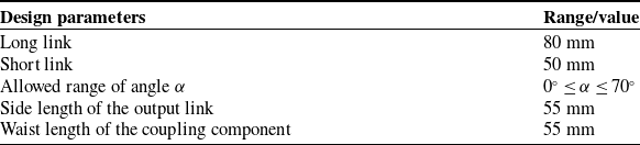
With the specific values of the parameters for the 3RR-3RRR MCM provided in Table II, each of the three 3RR-3RRR tetrahedral deployable units has an output link shaped as equilateral triangles and coupling components shaped as isosceles triangles.

Table II.

Prototype model parameters.

As shown in Figure 11, for material selection, each long/short link is made of T800H carbon fiber plates to achieve both lightweight design and structural stiffness. The output links and coupling components are 3D-printed with PLA material, ensuring dimensional accuracy while reducing revolute inertia. Bearings, bolts, and other standard parts are employed to minimize overall weight while maintaining required stiffness and strength. The inner ring of the bearing is wider than the outer ring, which is positioned by installing a spacer on the bolt on the outer side of the inner ring, and a lock nut is used to prevent loosening during rotation. The connection of the bearing is achieved through an interference fit between the mechanism links and the coupling parts. The bearing connections are realized through interference fits between mechanism links and coupling components. Positioning is achieved by installing spacers on bolts outside the inner rings, with lock nuts preventing loosening during rotation.

Figure 11.

3D exploded view of the link connections.

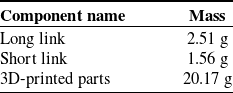
The masses of components within the mechanism are shown in Table III. In both actuation schemes, only the actuation input position of the motor is altered, with minimal impact on the overall mass of the mechanism. Each revolute joint is equipped with bearings to minimize friction; thus, the length of the moment arm and the mass of components connected to the motor significantly affect the motor torque. Based on the design parameters in Table II and component masses in Table III, a Maxon DCX-12L series miniature motor paired with a GPX-12 series planetary gearbox is selected. This compact motor configuration delivers relatively large output torque, fully meeting experimental requirements. Additionally, an ENX-10 encoder is chosen for feedback signals, with detailed motor parameters provided in Table IV.

Table III.

Prototype model mass.

Table IV.

Motor specifications.

The motor actuation is chosen to be the EPOS2 series digital position controller from Maxon. This controller allows real-time modification of control system parameters via PC software and visually reflects these parameters in the form of waveforms. The motor actuation is connected to the PC via a USB serial port, enabling it to receive output signals from the PC and feedback signals from the motor end to the PC. The specific parameters can be monitored in the upper computer software, and the system operation block diagram is shown in Figure 12.

Figure 12.

System operation block diagram.

6.2. Experimental validation

The previous section provided a theoretical examination of the mobility, singularity, and actuation selection schemes of the 3RR-3RRR MCM. The mobility is difficult to verify in experiments by means of numerical analysis. The singular positions are reflected in the workspace’s boundary, and the prototype can move smoothly except at the boundary. As a result, this part focuses on confirming the appropriate actuation choices via prototype experimental analysis. The actual power consumption of the motor during motion was measured by changing the output link motion trail, terminal load, and motion time under identical conditions. A lower actual power usage suggests lower energy consumption. The specific layout of the actuation motors for the two actuation schemes is shown in Figure 13.

Figure 13.

Physical diagram of the two actuation schemes. (a) Actuation scheme I. (b) Actuation scheme II.

To accurately assess the energy consumption differences between the actuation schemes, experiments were conducted under the condition of a motor torque≥0.4 and a load fluctuation ≤ 5%. A single-actuation joint was used to actuate the mechanism, while the remaining joints were set to a free-following state. This single-actuation configuration allowed the exclusion of multi-actuation coupling interference, thereby ensuring variable uniqueness in the comparative experiments and enhancing the clarity of result comparisons. The experimental platform comprised the following core modules: a PC host computer, a DC power supply, the test mechanism, and an actuation motor, as illustrated in Figure 14.

Figure 14.

Experimental platform.

To maintain the correctness of the experimental results, both actuation schemes were carried out on the same hexagonal base. Based on the mechanism analysis in the previous section and the actuation speed of the actuation joint calculated from the model parameters shown in Table II, the output connecting link was made to move along the same motion path within the same control time, enabling the overall mechanism to move from the same contracted state to the fully extended state. That is, as shown in Figure 6 (a), the singular configuration is reached and the motion stops simultaneously. The motion processes of the two selection schemes are shown in Figs. 15 and 16. According to the folding and unfolding states of the members between the modules (the red lines in the figure represent the members and the blue dots represent the revolute joints), it can be well observed which motion process the mechanism is in.

Figure 15.

Motion process of the mechanism with actuation scheme I. (a) Collapsed state. (b) Intermediate state. (c) Expanded state.

Figure 16.

Motion process of the mechanism with actuation scheme II. (a) Collapsed state. (b) Intermediate state. (c) Expanded state.

Under the condition that the constraints of the moving platform are the same, the corresponding current-time curves under the two actuation schemes are measured as shown in Figure 17. With a constant input voltage of 12 V, the actual power of the two actuation schemes is obtained as shown in Figure 18, and the results are compared with obvious effect, and the comparison yields that the actual power consumption of scheme I is lower, and the energy consumed under the first actuation scheme is smaller than that consumed under the second actuation scheme. Since the LTI value reflects the energy transfer efficiency, the scheme I demonstrates its superiority in the principle of energy optimization, with lower energy consumption and in line with the principle of energy optimization. This difference stems from the fact that the basic limb I, which is actuated by scheme I, is directly connected to the moving platform, which effectively reduces the inertial coupling effect during the movement of the mechanism, while scheme II is through the coupling limb. In addition, when the mechanism moves to the fully unfolded position, the measured speeds of all the actuation joints drop to zero synchronously, and the actuation motor current increases abruptly, triggering the overload protection of the system. This phenomenon indicates that the fully unfolded state is the actual dead point of the mechanism, where the moving platform loses all instantaneous DOFs. This configuration not only threatens the mechanism’s stability (e.g., motor overheating and mechanical jamming) but may also cause a loss of trajectory tracking control, which is entirely consistent with the theoretically predicted singular configuration.

Figure 17.

Current–time diagram. (a) Current–time diagram of actuation scheme I. (b) Current–time diagram of actuation scheme II.

Figure 18.

Power–time diagram.