1 Introduction
The time-dependent motion of a small spherical particle in a non-uniform Stokes flow can be described by the Maxey–Riley equation (Maxey & Riley Reference Maxey and Riley1983). Since 1983, a few studies have been conducted to extend the application of this equation to unsteady flows (Mei & Adrian Reference Mei and Adrian1992) and larger Reynolds number (Kim, Elghobashi & Sirignano Reference Kim, Elghobashi and Sirignano1998). However, the equation is still limited to the motion of a single sphere in a low
 $Re$
flow. Moreover, the Saffman (due to pressure distribution on the particle) and Magnus (due to particle rotation) lift forces, which are known to be important for large particles in turbulent flow have not been included in these equations (Crowe et al.
Reference Crowe, Schwarzkopf, Sommerfeld and Tsuji2012; Kim & Balachandar Reference Kim and Balachandar2012; Meller & Liberzon Reference Meller and Liberzon2015). These forces along with the wall repulsive force (Brenner Reference Brenner1961; Feng, Hu & Joseph Reference Feng, Hu and Joseph1994), particle–particle, and particle–wall collisions affect particle dynamics in turbulent particle-laden flow (Crowe et al.
Reference Crowe, Schwarzkopf, Sommerfeld and Tsuji2012). Therefore, to better model inertial particle motion in turbulent flows and support the continued development of numerical approaches, high-quality experimental data of particle dynamics for such flows are required. The latter can be obtained by measurement of particle acceleration through Lagrangian particle tracking techniques.
One of the first measurements of acceleration of inertial particles in a turbulent boundary layer was conducted by Gerashchenko et al. (Reference Gerashchenko, Sharp, Neuscamman and Warhaft2008). They recorded the two-dimensional trajectories of small (sub-Kolmogorov scale) airborne water droplets. The Stokes number (
 $St$
, the ratio of particle relaxation time to the flow time scale) of the droplets based on the Kolmogorov time-scale,
 $t_{K}$
, was in the range
 $0.035\leqslant St_{K}\leqslant 1.2$
at a small mass loading of 0.01 %. The droplets close to the wall were characterized as having an average streamwise deceleration (
 $\langle A_{x}\rangle <0$
, where
 $A_{x}$
is the instantaneous streamwise acceleration and
 $\langle \,\rangle$
is the ensemble average operator). Similar results were also obtained from numerical studies of turbulent particle-laden flows by Lavezzo et al. (Reference Lavezzo, Soldati, Gerashchenko, Warhaft and Collins2010), Zamansky, Vinkovic & Gorokhovski (Reference Zamansky, Vinkovic and Gorokhovski2011) and Yu, Vinkovic & Buffat (Reference Yu, Vinkovic and Buffat2016). These investigations used direct numerical simulation (DNS) for the fluid phase along with simplified versions of the Maxey–Riley equation for the solid phase. The numerical simulation of Lavezzo et al. (Reference Lavezzo, Soldati, Gerashchenko, Warhaft and Collins2010) was carried out for
 $0.87\leqslant St_{K}\leqslant 11.8$
, Zamansky et al. (Reference Zamansky, Vinkovic and Gorokhovski2011) for
 $1\leqslant St^{+}\leqslant 25$
(where
 $St^{+}$
is defined based on the inner time scale of the flow) and Yu et al. (Reference Yu, Vinkovic and Buffat2016) at
 $St^{+}=35$
. Each of these studies reported
 $\langle A_{x}\rangle <0$
in the near-wall region and related it to the dominant effect of viscous force on the particles. There is, however, a discrepancy in the values of the average wall-normal acceleration,
 $\langle A_{y}\rangle$
, as discussed below.
In the experiments of Gerashchenko et al. (Reference Gerashchenko, Sharp, Neuscamman and Warhaft2008), the droplets had
 $\langle A_{y}\rangle <0$
, with the positive axis pointing away from the wall. These droplets were sub-Kolmogorov, and had a high density ratio with respect to the carrier phase (
 ${\sim}833$
). Also, droplets do not rebound when they hit the wall, which is not the case for solid particles. The numerical simulations of Lavezzo et al. (Reference Lavezzo, Soldati, Gerashchenko, Warhaft and Collins2010) and Yu et al. (Reference Yu, Vinkovic and Buffat2016) also resulted in
 $\langle A_{y}\rangle <0$
for both unladen and particle-laden flows in the near-wall region while the Zamansky et al. (Reference Zamansky, Vinkovic and Gorokhovski2011) simulations showed that
 $\langle A_{y}\rangle >0$
. All these numerical simulations assumed point-wise particles and neglected the pressure distribution on the particle, near-wall lift, added-mass, and Basset forces. These forces are important when the particles are larger than the smallest scale of the flow (Calzavarini et al.
Reference Calzavarini, Volk, Lévêque, Pinton and Toschi2012). The aforementioned numerical studies also assumed elastic particle–wall interaction, and neglected wall repulsive forces and particle–particle collisions. Further development of the numerical simulations of turbulent particle-laden flows requires investigation of the effects of particle-related forces on their dynamics through collection and evaluation of experimental data.
The relationship between
 $St$
and particle acceleration has been previously investigated in turbulent flows to understand particle dynamics. The investigations have shown the remarkable effect of
 $St$
on the probability density function (p.d.f.) and root-mean-square (r.m.s.) of particle acceleration,
 $a$
. For example, Ayyalasomayajula et al. (Reference Ayyalasomayajula, Gylfason, Collins, Bodenschatz and Warhaft2006) analysed the effect of
 $St_{K}$
on the acceleration distribution of droplets in grid turbulence, which is isotropic. It was found that increasing
 $St_{K}$
from 0.09 to 0.15 narrowed the p.d.f. of
 $A_{x}$
and made its r.m.s. (i.e.
 $a_{x}$
) smaller. This trend was also reported by Bec et al. (Reference Bec, Biferale, Boffetta, Celani, Cencini, Lanotte, Musacchio and Toschi2006) who used DNS to investigate the effect of
 $St_{K}$
on the p.d.f. and r.m.s. of particles’ acceleration with
 $St_{K}<3.5$
in isotropic turbulent flows. The narrower tails of the acceleration p.d.f. and its smaller
 $a$
at higher
 $St_{K}$
in isotropic turbulence have been related to the effect of particle inertia on its motion; inertial particles are less responsive to the fluid motion and more likely to move out of vortices (where there are high acceleration motions) to regions with higher strain (Eaton & Fessler Reference Eaton and Fessler1994; Ayyalasomayajula et al.
Reference Ayyalasomayajula, Gylfason, Collins, Bodenschatz and Warhaft2006; Gerashchenko et al.
Reference Gerashchenko, Sharp, Neuscamman and Warhaft2008; Lavezzo et al.
Reference Lavezzo, Soldati, Gerashchenko, Warhaft and Collins2010).
In non-isotropic turbulence as would occur near a wall, a different relationship between
 $St_{K}$
and
 $a_{x}$
has been reported. For example, in the experimental study mentioned earlier, Gerashchenko et al. (Reference Gerashchenko, Sharp, Neuscamman and Warhaft2008) showed that increasing
 $St_{K}$
from 0.07 to 0.47 increased
 $a_{x}$
and suggested that this trend was because of the effect of gravity and mean shear on inertial particles. Lavezzo et al. (Reference Lavezzo, Soldati, Gerashchenko, Warhaft and Collins2010) conducted a DNS of particle-laden flow with and without gravity in non-isotropic turbulence to verify the effect of gravity on the relationship between
 $St_{K}$
and
 $a_{x}$
. The parameters of their simulation, including the particle/fluid density ratio and
 $St_{K}$
, were similar to those studied by Gerashchenko et al. (Reference Gerashchenko, Sharp, Neuscamman and Warhaft2008). In the study of Lavezzo et al. (Reference Lavezzo, Soldati, Gerashchenko, Warhaft and Collins2010), particles were able to collide with the wall and elastically rebound from it, in contrast to the droplets in the experiment of Gerashchenko et al. (Reference Gerashchenko, Sharp, Neuscamman and Warhaft2008). The comparison of the simulations of Lavezzo et al. (Reference Lavezzo, Soldati, Gerashchenko, Warhaft and Collins2010) with and without gravity confirmed that the increase in
 $a_{x}$
with increasing
 $St_{K}$
close to the wall is due to the combined effects of gravity and mean shear. They argued that the downward motion of the particles due to gravity exposes them to a strong deceleration due to the mean shear very close to the wall and causes high
 $a_{x}$
. The analysis of Lavezzo et al. (Reference Lavezzo, Soldati, Gerashchenko, Warhaft and Collins2010) showed that with increasing
 $St_{K}$
from 0.87 to 1.76, the
 $a_{x}$
slightly increased even in the absence of gravity (although this increase was small compared with that obtained when gravity was considered), followed by a continuous decrease in the value of
 $a_{x}$
as
 $St_{K}$
was increased from 1.76 to 11.8. This non-monotonic variation of
 $a_{x}$
with
 $St$
in the absence of gravity was also found in the numerical study of Zamansky et al. (Reference Zamansky, Vinkovic and Gorokhovski2011), who showed that in the near-wall, non-isotropic turbulence, the maximum value of
 $a_{x}$
increased when
 $St^{+}$
increased from 1 to 5, and then decreased for higher
 $St^{+}$
(up to
 $St^{+}=25$
). The results of the two numerical investigations indicate that other mechanisms in addition to gravity can decelerate the particles and increase
 $a_{x}$
. In particular, the effects of particle–wall interaction on acceleration statistics of inertial particles must be investigated.
The effects of particle–wall interactions have been studied experimentally under quiescent and flowing conditions. Joseph et al. (Reference Joseph, Zenit, Hunt and Rosenwinkel2001) measured the particle restitution coefficient (
 $e$
), defined as the ratio of particle velocity immediately after and before its collision with the wall, in fluids with different viscosities. Their experimental set-up consisted of a spherical particle attached to a string. This pendulum was released from different initial angles and moved through a quiescent liquid until the particle hit a vertical wall with an impact angle of
 $90^{\circ }$
. They defined the impact Stokes number,
 $St_{v}=\unicode[STIX]{x1D70C}_{p}d_{p}V_{0}/(9\unicode[STIX]{x1D707})$
, based on the particle’s wall-normal impact velocity (
 $V_{0}$
), particle diameter,
 $d_{p}$
, particle density,
 $\unicode[STIX]{x1D70C}_{p}$
and the dynamic viscosity of the fluid,
 $\unicode[STIX]{x1D707}$
. In their experiments, particle rebound did not occur (i.e.
 $e=0$
) when
 $St_{v}$
was below a critical value (
 $St_{v}\sim 10$
). At values
 $10<St_{v}<30$
, the coefficient
 $e$
rapidly increased with increasing
 $St_{v}$
(Joseph et al.
Reference Joseph, Zenit, Hunt and Rosenwinkel2001); however, with further increase in
 $St_{v}$
, values of
 $e$
increased more slowly and eventually asymptotically approached the value for dry collision (i.e. collision in air). The dependency of
 $e$
on
 $St_{v}$
is also reported by Gondret, Lance & Petit (Reference Gondret, Lance and Petit2002), Stocchino & Guala (Reference Stocchino and Guala2005) and Legendre et al. (Reference Legendre, Zenit, Daniel and Guiraud2006). Some other quiescent fluid studies also showed that
 $e$
depends on the impact angle,
 $\unicode[STIX]{x1D703}_{i}$
, which is defined as the angle between the particle trajectory and the wall. For example, Salman et al. (Reference Salman, Verba, Lukenics and Szabo1989, p. 31) tested particle–wall collisions in air and showed that an increase in
 $\unicode[STIX]{x1D703}_{i}$
reduced the wall-normal restitution coefficient (
 $e_{V}$
, defined as the ratio of the wall-normal velocity of a particle after and before the collision). This reduction was also observed by Joseph & Hunt (Reference Joseph and Hunt2004). The dependence of
 $e$
on
 $\unicode[STIX]{x1D703}_{i}$
in a turbulent flow of air was investigated by Sommerfeld & Huber (Reference Sommerfeld and Huber1999). They measured
 $e$
,
 $\unicode[STIX]{x1D703}_{i}$
, and rebound angle,
 $\unicode[STIX]{x1D703}_{r}$
, of spherical particles in air flowing through a horizontal rectangular channel. Their results also showed the reduction of
 $e$
with increasing
 $\unicode[STIX]{x1D703}_{i}$
. This reduction is also reported in a recent study by Sommerfeld & Lain (Reference Sommerfeld and Lain2018) for non-spherical particles in a turbulent air flow.
The dependence of
 $e$
on
 $\unicode[STIX]{x1D703}_{i}$
shows the important role this angle plays in particle–wall collision in turbulent flows. The motion of particles in non-isotropic turbulent flows strongly depends on the turbulent structures interacting with the particles (Kaftori, Hetsroni & Banerjee Reference Kaftori, Hetsroni and Banerjee1995a
,Reference Kaftori, Hetsroni and Banerjee
b
; Marchioli & Soldati Reference Marchioli and Soldati2002; Kiger & Pan Reference Kiger and Pan2002). For example, sweep and ejection motions affect particles’ flux toward and away from the wall (Nino & Garcia Reference Nino and Garcia1996; Soldati Reference Soldati2005), and quasi-streamwise vortices are known to cluster small particles along low-speed streaks (Nino & Garcia Reference Nino and Garcia1996). Knowledge of the distributions of
 $\unicode[STIX]{x1D703}_{i}$
and
 $e$
in a particle-laden turbulent flow is a key factor for modelling particle–wall interactions (Tsuji et al.
Reference Tsuji, Morikawa, Tanaka, Nakatsukasa and Nakatani1987; Sommerfeld & Huber Reference Sommerfeld and Huber1999; Kosinski & Hoffmann Reference Kosinski and Hoffmann2009; Sommerfeld & Lain Reference Sommerfeld and Lain2018).
In this study, we applied a time-resolved three-dimensional particle tracking velocimetry (3D-PTV) based on the shake-the-box (STB) algorithm of Schanz, Gesemann & Schröder (Reference Schanz, Gesemann and Schröder2016) to extract the Lagrangian trajectory of particles. This state-of-the-art particle tracking velocimetry method uses a few initial time steps to predict the particle location based on a polynomial fit of the particle trajectory. This prediction is corrected using an image matching technique, which involves ‘shaking’ the particles about their predicted location (Wieneke Reference Wieneke2013). As a result of this combined algorithm, accurate tracking of particles from two-dimensional images with up to 0.08 particles per pixel has become possible (Schröder et al.
Reference Schröder, Schanz, Michaelis, Cierpka, Scharnowski and Kähler2015; Schanz et al.
Reference Schanz, Gesemann and Schröder2016). The STB technique is used here to obtain trajectories, velocity and acceleration of inertial particles in a horizontal turbulent channel flow. The trajectories are also used to investigate the collision of the inertial particles with a wall, with specific attention paid to
 $\unicode[STIX]{x1D703}_{i}$
,
 $\unicode[STIX]{x1D703}_{r}$
and particle momentum exchange with the wall. The experimental set-up, data processing and the properties of the turbulent flow and the inertial particles are described in § 2. The accuracy of the measurement system and the processing algorithm is verified by comparing the measured velocity and acceleration statistics with DNS of unladen flow from Moser, Kim & Mansour (Reference Moser, Kim and Mansour1999) and Yeo, Kim & Lee (Reference Yeo, Kim and Lee2010) in § 3. The velocity and acceleration fields of the inertial particles are investigated in § 4. A quadrant analysis is performed in § 5 to study the contribution of turbulent motions to Reynolds stresses and acceleration of the inertial particles. The collision of the particles with the wall is investigated in § 6 using conditional averaging of particle velocity and acceleration based on the turbulent motions of particles and
 $\unicode[STIX]{x1D703}_{i}$
.
2 Experimental set-up
The experiments are conducted in a closed flow loop with a transparent test section constructed specifically for 3D-PTV measurements. The ability of the STB algorithm in simultaneous recording of the trajectories of a large number of particles across the measurement domain with high accuracy makes it a desirable method for the Lagrangian tracking of particles (Toschi & Bodenschatz Reference Toschi and Bodenschatz2009) and measurement of their acceleration in turbulent particle-laden flows. Descriptions of the flow facility, the test conditions and the 3D-PTV system are provided in the following sections.
2.1 Flow facility
The closed horizontal flow-loop consisted of 2 in. (nominal) diameter pipe and included a 3 m long rectangular test section as shown in figure 1. The test cross-section had dimensions of
 $(W\times 2H)=120\times 15~\text{mm}^{2}$
(where
 $H$
is the channel half-height) and thus a hydraulic diameter of
 $D_{h}=26.7$
mm. The test section was connected to the pipes using two gradual transition sections with 30 cm length. The measurement location was
 $220H$
from the entrance of the rectangular section to ensure fully developed turbulent flow. The test section had glass walls for optical access, which were also removable to calibrate the 3D-PTV system. A centrifugal pump (LCC-Metal, GIW Industries Inc.) circulated the flow inside the flow loop. The flow rate and the temperature were measured using a Coriolis flowmeter (Micro Motion F-Series, Emerson Industries) with mass flow accuracy of 0.2 %. The pump was isolated from the test section using rubber joints so that vibrations from the pump or flow loop do not affect the optical measurements. The temperature of the flow was kept constant at
 $20\,^{\circ }\text{C}$
for all the measurements using a double-pipe heat exchanger. All experiments were performed at
 $Re_{H}=14\,600$
, based on the channel height and the bulk velocity across the channel (
 $U_{b}=0.98~\text{m}~\text{s}^{-1}$
), which corresponded to a mass flow rate of
 $1.76~\text{kg}~\text{s}^{-1}$
. The friction velocity of the unladen flow was
 $u_{\unicode[STIX]{x1D70F}}=0.0548~\text{m}~\text{s}^{-1}$
, meaning the friction Reynolds number of
 $Re_{\unicode[STIX]{x1D70F}}=u_{\unicode[STIX]{x1D70F}}H/\unicode[STIX]{x1D710}=410$
. The wall-normal unit was
 $\unicode[STIX]{x1D706}=18.3~\unicode[STIX]{x03BC}\text{m}$
, estimated from the 3D-PTV measurements as discussed in § 3. The main flow parameters are shown in table 1.
The 18 m (length) by 0.054 m (diameter) flow loop used in the present study, which includes a transparent channel with a rectangular test section used for optical measurements.

The flow parameters describing the unladen flow. The inner scaling is calculated from the velocity profile measured using the 3D-PTV technique.

2.2 Particle-laden flow characteristics
The particle-laden flow consisted of narrowly sized glass beads with mean diameter of
 $d_{p}=125~\unicode[STIX]{x03BC}\text{m}$
and density of
 $\unicode[STIX]{x1D70C}_{p}=2.5~\text{g}~\text{cm}^{-3}$
dispersed in water at a volumetric concentration of
 $C_{v}=0.03\,\%$
, equivalent to a mass fraction of
 $C_{m}=0.1\,\%$
. For these glass beads and the test conditions under which they were studied,
 $St^{+}=3.9$
, where
 $St^{+}$
was defined as the ratio of the bead relaxation time to the inner time scale of the flow (
 $t_{p}/t_{f}$
). The time scales were estimated as
 $t_{p}=(\unicode[STIX]{x1D70C}_{p}-\unicode[STIX]{x1D70C}_{f})d_{p}^{2}/18\unicode[STIX]{x1D707}$
and
 $t_{f}=\unicode[STIX]{x1D710}/u_{\unicode[STIX]{x1D70F}}^{2}$
where
 $\unicode[STIX]{x1D70C}_{f}$
and
 $\unicode[STIX]{x1D710}$
are the density and kinematic viscosity of the fluid, respectively. The
 $St$
can also be determined based on the Kolmogorov time scale,
 $t_{K}$
. The Kolmogorov time scale is estimated as
 $t_{K}=(\unicode[STIX]{x1D710}/\unicode[STIX]{x1D700})^{0.5}$
where
 $\unicode[STIX]{x1D700}=C_{\unicode[STIX]{x1D707}}^{0.75}k^{1.5}/l_{m}$
. Here,
 $k$
is the turbulent kinetic energy,
 $l_{m}$
is turbulent mixing length and
 $C_{\unicode[STIX]{x1D707}}=0.09$
(Milojevié Reference Milojevié1990). Turbulent mixing length can be estimated using the
 $l_{m}=\unicode[STIX]{x1D705}y(1-y/(2H))^{0.5}$
, where
 $\unicode[STIX]{x1D705}=0.4$
is the von Kármán constant (Prandtl Reference Prandtl1932). Based on the values of
 $k$
and
 $l_{m}$
at
 $y=4$
mm (the farthest available data point from the bottom wall),
 $t_{K}$
is approximately 5 ms. Therefore, the lower bound of the glass bead’s
 $St_{K}$
in the measurement domain is 0.2.
The Reynolds number for glass beads can be defined as
 $Re_{p}=U_{s}d_{p}/\unicode[STIX]{x1D710}$
, where
 $U_{s}$
is the streamwise slip velocity of the beads. From the 3D-PTV measurement (discussed in § 3), the mean streamwise velocity of unladen flow,
 $\langle U_{f}\rangle$
, and the beads’ mean velocity,
 $\langle U_{p}\rangle$
, can be measured. These values are used to estimate
 $U_{s}$
as
 $|\langle U_{f}\rangle -\langle U_{p}\rangle |$
. Using this equation, the maximum
 $Re_{p}$
in the measurement domain is approximately 11.2. This maximum
 $Re_{p}$
is an order of magnitude less than the threshold of
 $Re_{p}=110$
, suggested for vortex shedding from spherical particles (Hetsroni Reference Hetsroni1989). The properties of the glass beads studied here are summarized in table 2. It should be expected that the inertia will have a considerable effect on the dynamics of the glass beads since
 $St^{+}>1$
(Aliseda et al.
Reference Aliseda, Cartellier, Hainaux and Lasheras2002). Particle–particle collisions were not expected to play a significant role at this concentration (Elghobashi Reference Elghobashi1994).
Properties of the glass beads used as inertial particles tested in the present study.

From a comparison of
 $C_{m}$
(0.1 %) and
 $d_{p}^{+}$
(6.8) of the current investigation with previous studies, the effect of glass beads on the turbulent structures of the fluid phase is expected to be negligible, i.e. a marginal two-way coupling. The experimental results of Kulick, Fessler & Eaton (Reference Kulick, Fessler and Eaton1994) showed that
 $90~\unicode[STIX]{x03BC}\text{m}$
glass beads with
 $C_{m}$
of 2 % and
 $d_{p}^{+}$
of 3 had a negligible effect on the turbulent intensity of the carrier phase. The numerical analysis of Nasr & Ahmadi (Reference Nasr and Ahmadi2007) for particles with
 $d_{p}^{+}$
of 2.2 and
 $C_{m}=2\,\%$
also showed a negligible change of the flow turbulent kinetic energy and dissipation. In Kulick et al. (Reference Kulick, Fessler and Eaton1994) and Nasr & Ahmadi (Reference Nasr and Ahmadi2007), the carrier phase was air, which has a higher
 $r_{\unicode[STIX]{x1D70C}}$
relative to the current study. Therefore, the smaller
 $r_{\unicode[STIX]{x1D70C}}$
of the present investigation is expected to result in an even smaller modulation of flow turbulence (Yu et al.
Reference Yu, Lin, Shao and Wang2017). Regarding the finite size of the beads, DNS of Luo et al. (Reference Luo, Hu, Wu and Fan2017) for particles with
 $d_{p}^{+}$
of 11.3 (without point-particle assumption),
 $r_{\unicode[STIX]{x1D70C}}$
of 3.3 and
 $C_{v}$
of 0.1 % showed a negligible effect on fluid turbulence. This observation was made in spite of turbophoresis and a larger near-wall particle concentration in their study.
2.3 Lagrangian 3D-PTV measurements
A time-resolved 3D-PTV system was used to obtain glass bead trajectories based on the STB algorithm (Schanz et al.
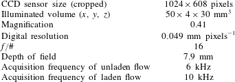
Reference Schanz, Gesemann and Schröder2016). The system consisted of four CMOS high-speed cameras (Phantom v611) with a pixel size of
 $20\times 20~\unicode[STIX]{x03BC}\text{m}^{2}$
operated at a cropped sensor size of
 $1024\times 608$
pixels. Each camera was equipped with a Scheimpflug adaptor and a Sigma SLR objective lens with a focal length of
 $f=105$
mm at an aperture size of
 $f/16$
. The magnification of the imaging system was 0.41 at a digital resolution of
 $0.049~\text{mm}~\text{pixels}^{-1}$
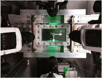
and depth-of-field of 7.9 mm. The cameras were arranged in a plus-like configuration with solid-angle of
 ${\sim}35^{\circ }$
from the
 $y$
-axis as shown in figure 2. The cameras were synchronized with a dual cavity Nd : YLF laser (DM20-527, Photonics Industries) through a high-speed controller (HSC v2, LaVision GmbH) controlled by DaVis 8.4 (LaVision GmbH). The laser had a wavelength of 527 nm and each cavity had maximum energy of 20 mJ per pulse (at frequency of 1 kHz). A combination of cylindrical and spherical lenses was used to collimate the laser beam into a sheet with cross-section of
 $50\times 4~\text{mm}^{2}$
in the streamwise (
 $x$
) and wall-normal (
 $y$
) directions. The laser sheet entered the test section from the sidewall, passed parallel to the bottom wall, and exited from the opposite sidewall (from top to bottom in figure 2). To increase the laser intensity a mirror was used on the opposite side (after the test section) to reflect the laser back into the measurement volume. Two knife-edges were used outside the sidewalls to form a top-hat intensity profile and limit the laser sheet in the region
 $0\leqslant y\leqslant 4$
mm. The
 $y$
-axis points in the wall-normal direction from the bottom wall toward the top wall with
 $y=0$
at the bottom wall. The centre of the coordinate system was located at the centre of the bottom wall of the test section as shown in figure 2. The flow was in the positive
 $x$
direction and the
 $z$
-axis indicates the spanwise direction.
An image of the high-speed 3D-PTV system showing the four cameras imaging the test section in a plus-like configuration. The laser sheet is reflected back into the test section using a mirror to increase the light intensity and to equalize the image intensity of the cameras in backward and forward scattering orientations (Ghaemi & Scarano Reference Ghaemi and Scarano2010).

A third-order polynomial function was obtained using a three-dimensional (3-D) target to calibrate the imaging system and map the physical coordinate system on the image coordinate system. The calibration errors were reduced to 0.05 pixel by applying a volume self-calibration algorithm of Wieneke (Reference Wieneke2008) in DaVis 8.4 (LaVision GmbH). The average disparity error in the whole measurement domain was approximately 0.01 pixel with standard deviation of 0.01 pixel. The reported disparity error is an order of magnitude smaller than the maximum recommended value of 0.1 pixel by Wieneke (Reference Wieneke2008). The measurement volume was
 $50\times 4\times 30~\text{mm}^{3}$
, which was equivalent to
 $1024\times 82\times 608~\text{pixels}^{3}$
. Image acquisition was at a speed of 6 kHz for the unladen flow measurements and 10 kHz for particle-laden measurements. In each case, the system was set to single-frame mode with simultaneous emission of the two laser cavities. The acquisition rate was higher for the particle-laden flow tests to better resolve the bead–wall collision process. The time interval between laser pulses was 167 and
 $100~\unicode[STIX]{x03BC}\text{s}$
for the unladen and bead-laden measurements, respectively, or approximately half and one-third of the inner time scale of the flow (
 $t_{f}=337~\unicode[STIX]{x03BC}\text{s}$
). The specifications of the 3D-PTV set-up are detailed in table 3. The unladen flow was seeded with
 $2~\unicode[STIX]{x03BC}\text{m}$
silver-coated tracers (SG02S40 Potters Industries) with a density of
 $3.6~\text{g}~\text{cm}^{-3}$
. The tracers had an image size of 3 pixels, their volumetric number density was
 $3~\text{tracer}~\text{mm}^{-3}$
, and the number density of the tracers in the images was 0.024 tracer per pixel. The maximum displacement of the tracers for unladen flow measurements did not exceed 4 pixels between two consecutive images. In the bead-laden flow (no tracer), the
 $125~\unicode[STIX]{x03BC}\text{m}$
glass beads had a Gaussian intensity profile and image diameter of
 ${\sim}3$
pixels. The number density of beads was 0.825 beads per cubic millimetre at volumetric concentration of 0.03 %. The number density of beads in the images was 0.008 beads per pixel. The maximum displacement of beads was
 ${\sim}2$
pixels between two consecutive images.
Specifications of the 3D-PTV system used in the present study.

After recording the images, the minimum intensity of the ensemble of images was subtracted from each image to remove the background. The signal-to-noise ratio of the images was also improved by subtracting the minimum intensity within a kernel of five pixels from each pixel, and normalizing it using the average intensity within a kernel of 50 pixels. The image intensity of the cameras was also normalized with respect to each other, and a Gaussian filter with kernel of
 $3\times 3$
pixel was applied. An optical transfer function (known as an OTF) was obtained and applied in every step of iterative particle reconstruction and the shaking as described by Schanz et al. (Reference Schanz, Gesemann and Schröder2016). The data were processed using the STB algorithm in DaVis 8.4 (LaVision, GmbH) to determine the 3-D trajectory of each tracer in unladen flow and each bead in bead-laden flow. In this algorithm, the 3-D location of each particle is initially determined based on particle intensity, an allowed triangulation error, and a prediction of particle location from the previous images. The deviation of the predicted location is corrected by shaking the particle around the predicted location in small increments, and calculating the residual intensity following the iterative particle reconstruction method (Wieneke Reference Wieneke2013). The allowed triangulation error was 0.5 pixel (
 $24.5~\unicode[STIX]{x03BC}\text{m}$
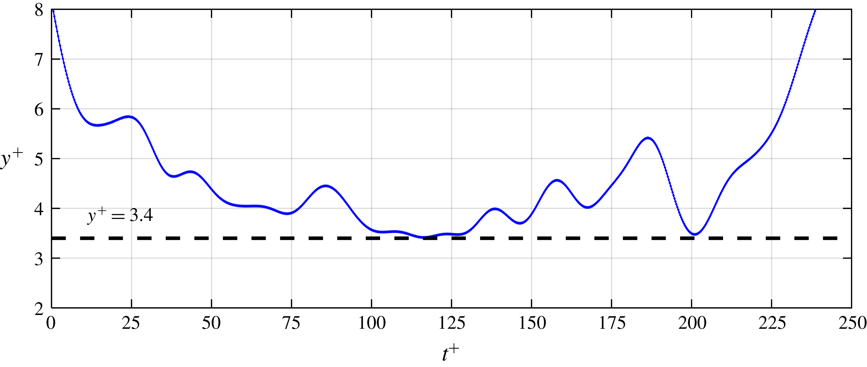
) and the shake width was 0.1 voxel. To avoid spurious results, the maximum allowable displacement was 4 voxels for the tracers and 3 voxels for beads. The maximum absolute and relative changes in the particle displacement between two consecutive images were limited to 2 pixel and 50 %, respectively. The STB algorithm detected approximately 300 tracer trajectories and approximately 50 bead trajectories per image for the unladen and the bead-laden experiments, respectively. Visualization of a sample trajectory of a bead is presented in figure 3 showing its wall-normal location normalized by the inner length-scale (
 $y^{+}=y/\unicode[STIX]{x1D706}$
) as a function of time, which is also normalized by the inner time scale (
 $t^{+}=t/t_{f}$
). The bead slides along the wall over a time period of
 $115\leqslant t^{+}\leqslant 130$
and the sharpest wall collision angle is at
 $t^{+}\approx 200$
.
The location of the lower wall was obtained using the minimum intensity of all the images. This minimum image was mostly dark, except for a few glare points due to the reflection of laser from the wall. To find the 3-D position of the glare point, i.e. wall location, the minimum image was reconstructed into the 3-D domain using the multiplicative algebraic reconstruction technique (known as MART) in DaVis 8.4 (Elsinga et al.
Reference Elsinga, Scarano, Wieneke and Van Oudheusden2006). The average intensity of the glare points was determined in each reconstructed
 $x$
–
 $z$
plane. A Gaussian distribution was fitted on the wall-normal variation of glare points’ intensity to obtain the wall location with subpixel accuracy. Based on this procedure the uncertainty of the wall-location is 0.1 pixel (
 $4.9~\unicode[STIX]{x03BC}\text{m}$
) which is equivalent to
 $0.27\unicode[STIX]{x1D706}$
.
Visualization of a bead trajectory showing multiple interactions with the wall. The dashed line shows
 $y^{+}=d_{p}^{+}/2$
which is the minimum
 $y$
that the centre of the bead can reach. The bead is sliding on the wall at
 $115\leqslant t^{+}\leqslant 130$
and has a relatively steep-angle collision with the wall at
 $t^{+}\approx 200$
.

The streamwise, wall-normal and spanwise instantaneous velocities (
 $U$
,
 $V$
,
 $W$
), velocity fluctuations (
 $u$
,
 $v$
,
 $w$
), instantaneous acceleration (
 $A_{x}$
,
 $A_{y}$
,
 $A_{z}$
) and r.m.s. of acceleration components (
 $a_{x}$
,
 $a_{y}$
,
 $a_{z}$
) were determined from the 3-D Lagrangian trajectories. The velocity and acceleration were obtained by applying a quadratic regression fit with temporal kernel of 4.5 ms (
 ${\sim}13t_{f}$
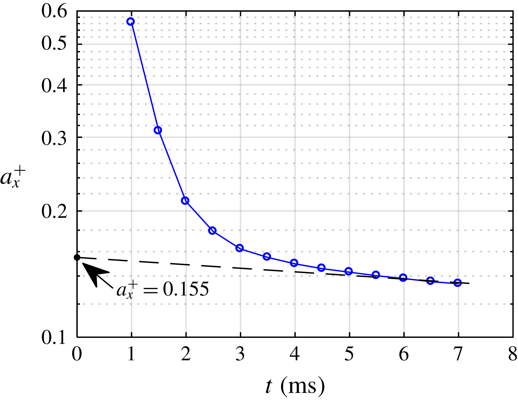
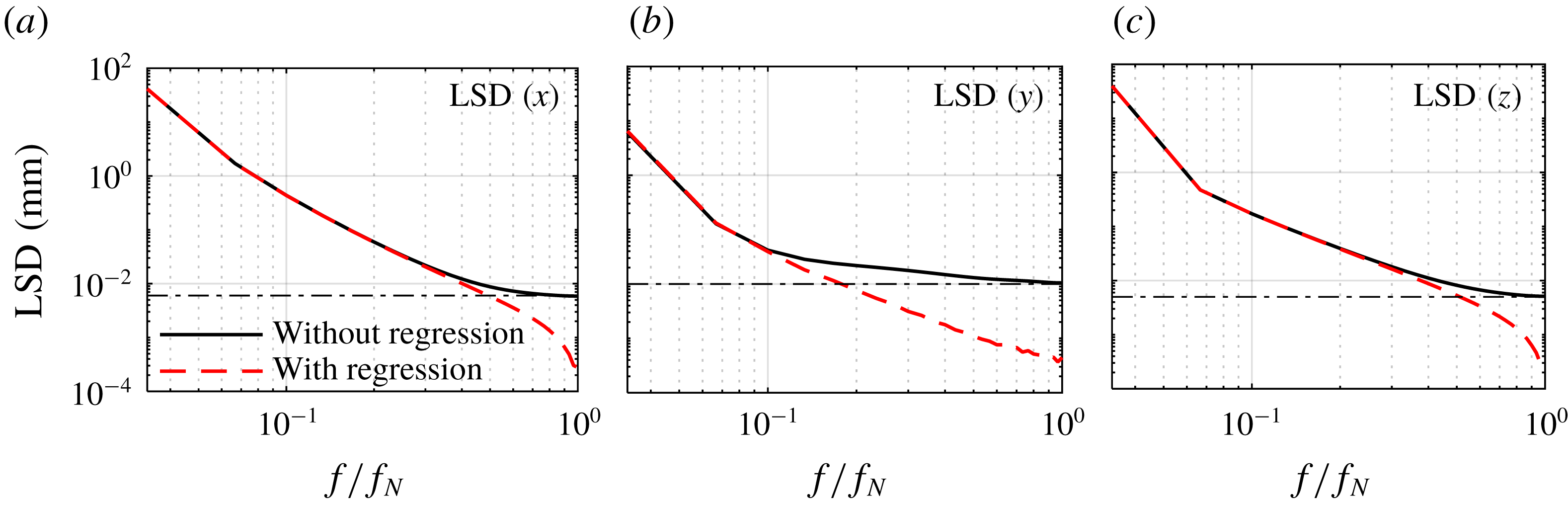
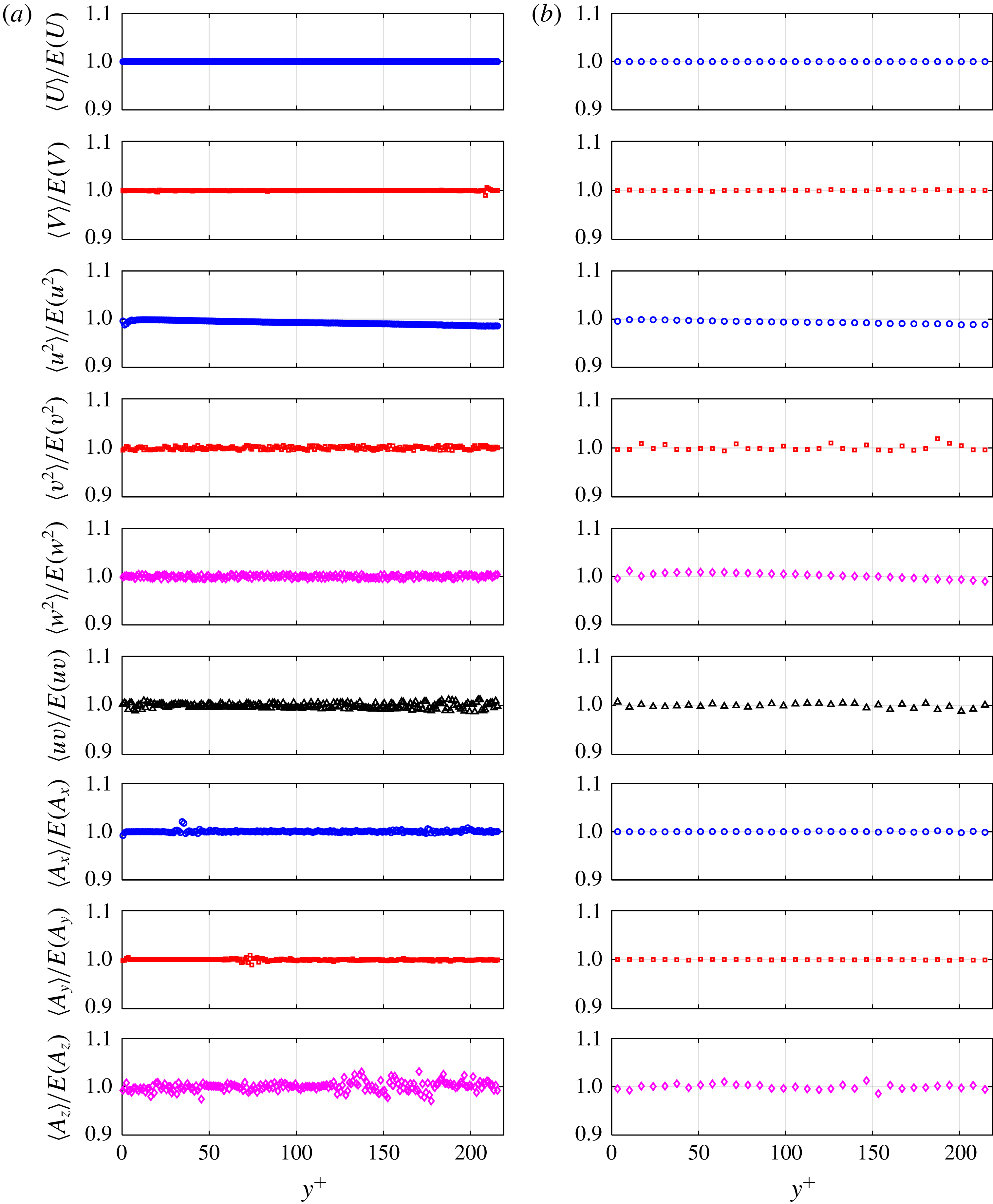
) on either the tracer or the bead trajectories. The kernel size was evaluated by comparing the velocity and acceleration statistics of unladen flow with the DNS results of Moser et al. (Reference Moser, Kim and Mansour1999) and Yeo et al. (Reference Yeo, Kim and Lee2010). The effect of the temporal kernel on the r.m.s. of acceleration values was evaluated following the method of Voth et al. (Reference Voth, La Porta, Crawford, Alexander and Bodenschatz2002) and Gerashchenko et al. (Reference Gerashchenko, Sharp, Neuscamman and Warhaft2008), and is shown in appendix A. The velocity and acceleration data were averaged in the streamwise and spanwise direction (in addition to time) due to homogeneity of the flow field in these directions. The ensemble averaged quantities are indicated using the
 $\langle \,\rangle$
symbol. The wall-normal dimension of the averaging bins was one wall unit,
 $\unicode[STIX]{x1D706}$
, for the unladen flow. The bin size was larger and equal to the diameter of a bead (
 $6.83\unicode[STIX]{x1D706}$
) for the bead-laden flow. More than
 $9\times 10^{6}$
tracer trajectories for unladen flow from 27 000 images (at 6 kHz) and approximately
 $2.3\times 10^{6}$
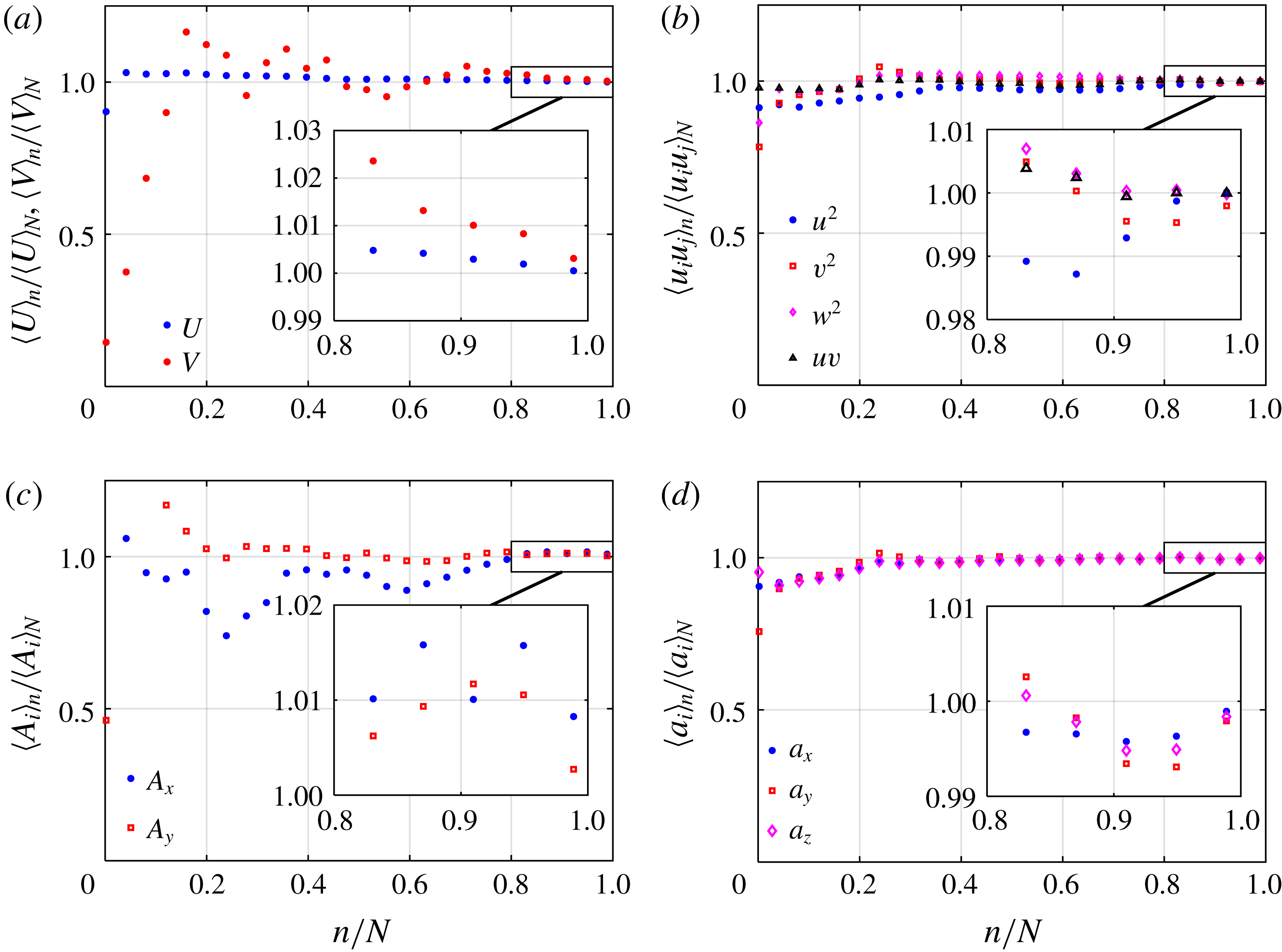
bead trajectories in the bead-laden flow from 45 000 images (at 10 kHz) were obtained using the STB algorithm. The convergence of the velocity and acceleration statistics of beads at
 $y^{+}=16.7$
, where
 $\langle u^{2}\rangle$
was a maximum, is investigated in appendix B. The random errors in measurement of velocity and acceleration statistics of glass beads were calculated based on the standard deviation of the last 20 % of data collected at this location and are presented in table 4. The mean duration of bead trajectories is relatively constant and is approximately 20 ms for
 $y^{+}>20$
. For smaller
 $y^{+}$
, the mean trajectory duration gradually shortens to approximately 13 ms.
Random errors of the velocity and acceleration statistics of glass beads based on the standard deviation of the last 20 % of data collected at
 $y^{+}=16.7$
. The details are available in appendix B.

3 Unladen turbulent channel flow
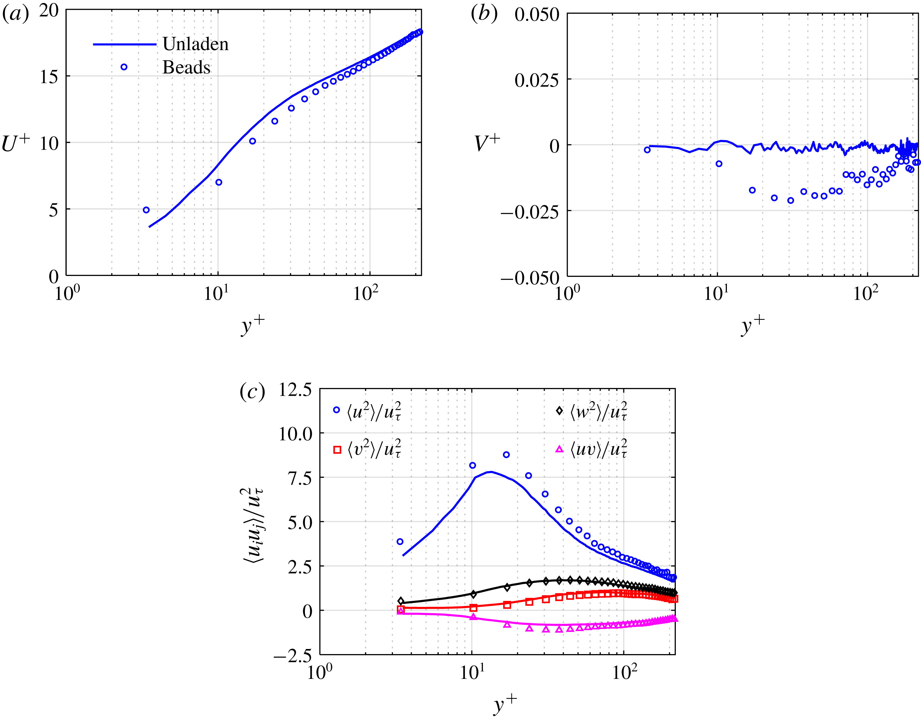
The unladen flow field statistics and the uncertainty of the 3D-PTV technique are evaluated by comparing the velocity statistics with the DNS results of Moser et al. (Reference Moser, Kim and Mansour1999) at
 $Re_{\unicode[STIX]{x1D70F}}=395$
and the acceleration statistics with a separate DNS study of Yeo et al. (Reference Yeo, Kim and Lee2010) at
 $Re_{\unicode[STIX]{x1D70F}}=408$
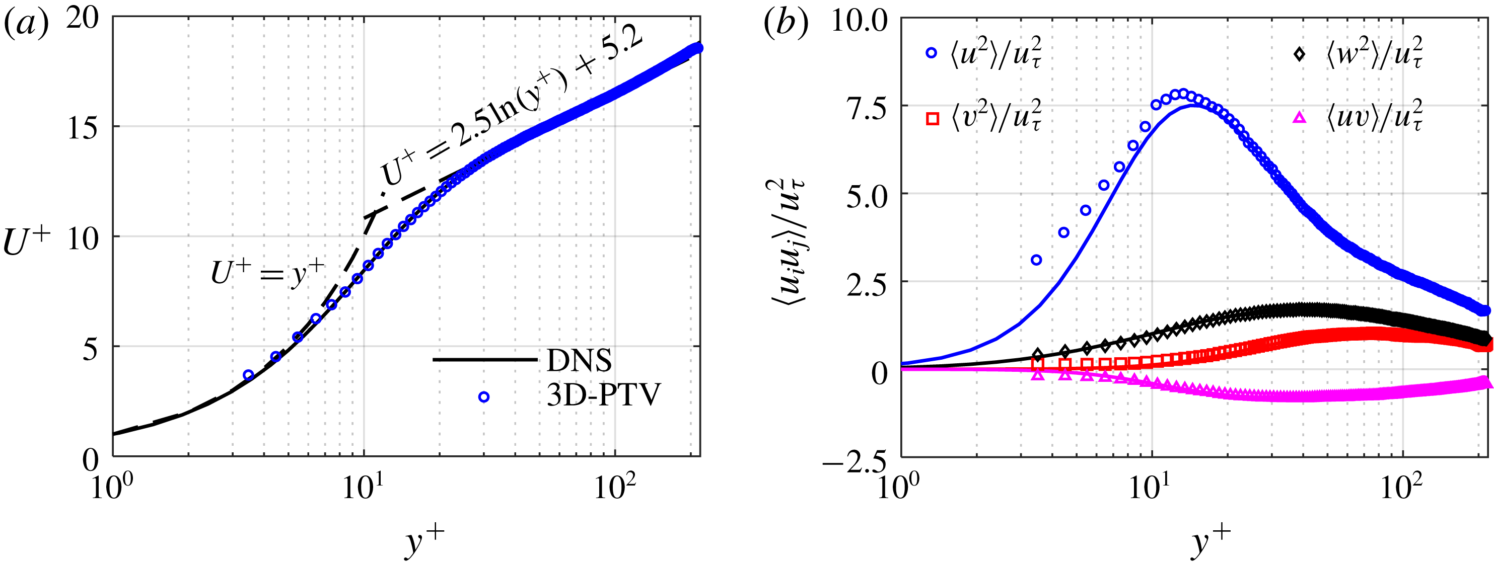
. The normalized mean streamwise velocity (
 $U^{+}$
), where
 $U^{+}=\langle U\rangle /u_{\unicode[STIX]{x1D70F}}$
, is shown here as figure 4(a). The 3D-PTV measurement agrees well with the DNS results of Moser et al. (Reference Moser, Kim and Mansour1999) from the first data point at
 $y^{+}=3.4$
in the viscous sublayer up to the border of the measurement volume at
 $y^{+}=218$
(
 $y=4$
mm) in the logarithmic region. The logarithmic law (
 $U^{+}=1/\unicode[STIX]{x1D705}\ln (y^{+})+B$
) with
 $\unicode[STIX]{x1D705}=0.4$
and
 $B=5.2$
is also shown in this figure.
Comparison of 3D-PTV measurement of (a) mean streamwise velocity, and (b) non-zero components of Reynolds stress tensor in unladen flow at
 $Re_{\unicode[STIX]{x1D70F}}=410$
(symbols) with the DNS results of Moser et al. (Reference Moser, Kim and Mansour1999) at
 $Re_{\unicode[STIX]{x1D70F}}=395$
(solid lines).

The non-zero components of the Reynolds stress tensor,
 $\langle \unicode[STIX]{x1D636}_{i}\unicode[STIX]{x1D636}_{j}\rangle$
, determined from 3D-PTV measurement, are shown in figure 4(b). The mean streamwise Reynolds stress profile,
 $\langle u^{2}\rangle$
, at the near-wall region of
 $y^{+}\leqslant 12$
is slightly larger (4 % in the peak) than the DNS results, and the maximum is also closer to the wall by
 ${\sim}2\unicode[STIX]{x1D706}$
. The difference can be partly attributed to the fact that the measurement was made at
 $Re_{\unicode[STIX]{x1D70F}}=410$
which results in a thinner inner layer and slightly larger values of
 $\langle u^{2}\rangle /u_{\unicode[STIX]{x1D70F}}^{2}$
than the Moser et al. (Reference Moser, Kim and Mansour1999) simulation, where
 $Re_{\unicode[STIX]{x1D70F}}=395$
. The profiles of mean wall-normal Reynolds stress,
 $\langle v^{2}\rangle$
, and mean spanwise Reynolds stress,
 $\langle w^{2}\rangle$
, overlap the DNS results and reach their maximum values at
 $y^{+}=70$
and 40, respectively. The mean Reynolds shear stress,
 $\langle uv\rangle$
, also agrees well with the DNS data, and the minimum value is reached at
 $y^{+}=35$
. The good agreement of the measurement with the DNS results also provides evidence indicating that (i) fully developed channel flow is established and (ii) the 3D-PTV can resolve the mean and second-order velocity statistics in the region
 $3.5\leqslant y^{+}\leqslant 218$
.
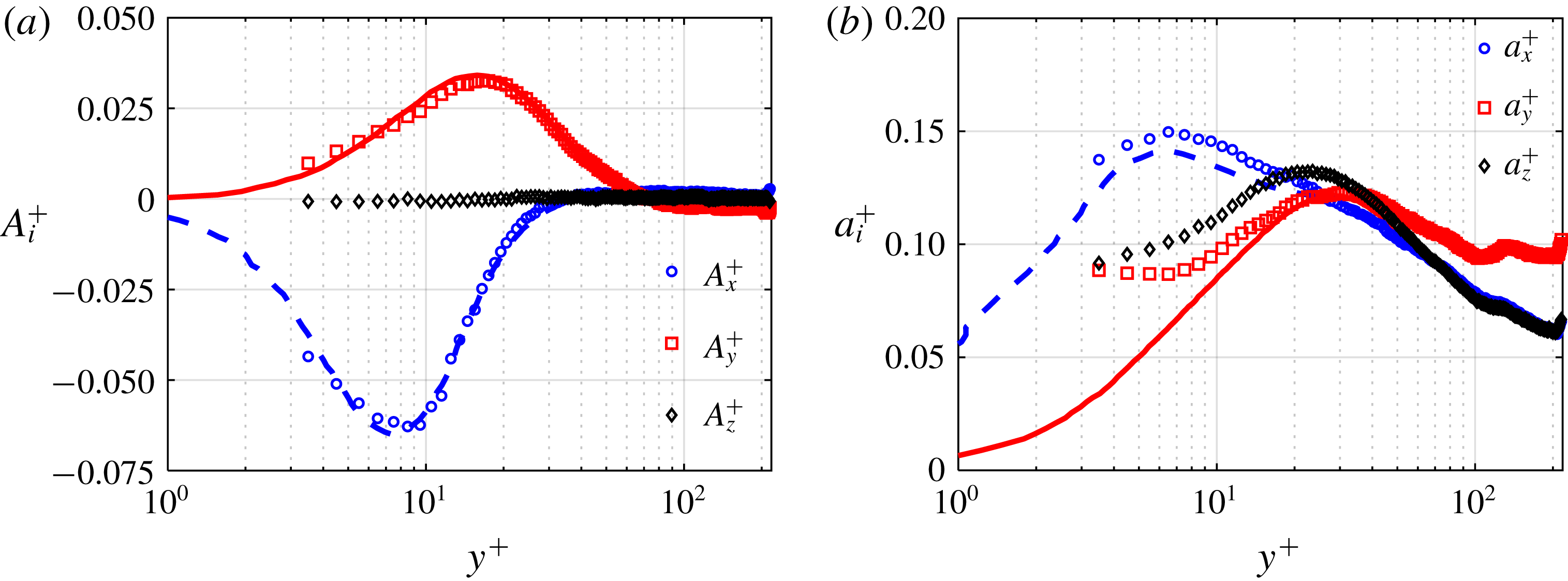
The ability of the 3D-PTV technique in resolving the mean and second-order acceleration statistics is investigated by comparing the results of the measurement made for the unladen flow with the DNS results of Yeo et al. (Reference Yeo, Kim and Lee2010) at
 $Re_{\unicode[STIX]{x1D70F}}=408$
. The profiles of normalized mean streamwise acceleration
 $A_{x}^{+}=\langle A_{x}\rangle /(u_{\unicode[STIX]{x1D70F}}^{3}/\unicode[STIX]{x1D710})$
and mean wall-normal acceleration,
 $A_{y}^{+}$
, and mean spanwise acceleration,
 $A_{z}^{+}$
, are presented in figure 5(a) for the unladen flow. The measurements of
 $A_{x}^{+}$
and
 $A_{y}^{+}$
show good agreement with the DNS. At the locations where the minimum value of
 $A_{x}^{+}$
and the maximum value of
 $A_{y}^{+}$
occur (
 $y^{+}=8$
and 18, respectively), the difference between the experimental and simulation results is approximately 4 %. At
 $y^{+}<35$
,
 $A_{x}^{+}$
is negative, which indicates flow deceleration. Yeo et al. (Reference Yeo, Kim and Lee2010) attributed the negative value of
 $A_{x}^{+}$
in the near-wall region mainly to the viscous force within the solenoidal acceleration (
 $\equiv \unicode[STIX]{x1D710}\unicode[STIX]{x2202}^{2}\langle U\rangle /\unicode[STIX]{x2202}y^{2}$
). The negative
 $A_{x}^{+}$
at
 $y^{+}<35$
is also expected because
 $\langle A_{x}\rangle \equiv \unicode[STIX]{x2202}\langle uv\rangle /\unicode[STIX]{x2202}y$
(Chen et al.
Reference Chen, Coleman, Vassilicos and Hu2010). As it is well known, and seen in figure 4(b),
 $\unicode[STIX]{x2202}\langle uv\rangle /\unicode[STIX]{x2202}y<0$
in this region. At
 $y^{+}<70$
,
 $A_{y}^{+}$
is positive as shown in figure 5(a). This agrees with the DNS results of Yeo et al. (Reference Yeo, Kim and Lee2010) at
 $Re_{\unicode[STIX]{x1D70F}}=[180,408,600]$
and the DNS results of Zamansky et al. (Reference Zamansky, Vinkovic and Gorokhovski2011) at
 $Re_{\unicode[STIX]{x1D70F}}=587$
. The positive values of
 $A_{y}^{+}$
at
 $y^{+}<70$
is also expected since
 $\langle A_{y}\rangle \equiv \unicode[STIX]{x2202}\langle v^{2}\rangle /\unicode[STIX]{x2202}y$
(Chen et al.
Reference Chen, Coleman, Vassilicos and Hu2010) and
 $\unicode[STIX]{x2202}\langle v^{2}\rangle /\unicode[STIX]{x2202}y$
is positive up to
 $y^{+}\approx 70$
as observed in figure 4(b). The variation of
 $A_{y}^{+}$
with
 $y^{+}$
also agrees with the variation of
 $\unicode[STIX]{x2202}\langle v^{2}\rangle /\unicode[STIX]{x2202}y$
with
 $y^{+}$
in figure 4(b). However, the trend of the values of
 $A_{y}^{+}$
measured for the present study is not in agreement with the DNS results of Lavezzo et al. (Reference Lavezzo, Soldati, Gerashchenko, Warhaft and Collins2010) at
 $Re_{\unicode[STIX]{x1D70F}}=300$
or Yu et al. (Reference Yu, Vinkovic and Buffat2016) at
 $Re_{\unicode[STIX]{x1D70F}}=150$
, who reported negative
 $A_{y}^{+}$
values near the bottom wall of horizontal channel flows. The positive
 $A_{y}^{+}$
in the inner layer is attributed to the irrotational component of
 $\langle A_{y}\rangle$
(
 $\equiv -\unicode[STIX]{x2202}\langle p\rangle /\unicode[STIX]{x1D70C}\unicode[STIX]{x2202}y$
) that accelerates the flow upward toward the axis of rotation of quasi-streamwise vortices (Lee, Yeo & Choi Reference Lee, Yeo and Choi2004; Lee & Lee Reference Lee and Lee2005; Yeo et al.
Reference Yeo, Kim and Lee2010). The rotational motion of the quasi-streamwise vortices provides a mean low-pressure core at
 $y^{+}\approx 20$
(Kim, Moin & Moser Reference Kim, Moin and Moser1987). This is consistent with the location of the maximum value of
 $A_{y}^{+}$
at
 $y^{+}=18$
in figure 5(a). The trends of the wall-normal variation of
 $\langle A_{x}\rangle$
and
 $\langle A_{y}\rangle$
of the unladen flow in the current study are also consistent with the experimental and DNS results of Stelzenmuller et al. (Reference Stelzenmuller, Polanco, Vignal, Vinkovic and Mordant2017). For a spanwise homogeneous flow,
 $A_{z}^{+}$
is expected to be zero. The maximum deviation of
 $A_{z}^{+}$
from zero is approximately
 $7.3\times 10^{-4}$
and occurs at
 $y^{+}=4.5$
, which is an indication of small measurement uncertainty.
The 3D-PTV measurement (symbols) of (a) mean acceleration, and (b) r.m.s. of acceleration for the unladen flow at
 $Re_{\unicode[STIX]{x1D70F}}=410$
. The results are normalized with inner scaling and compared with the DNS results of Yeo et al. (Reference Yeo, Kim and Lee2010) at
 $Re_{\unicode[STIX]{x1D70F}}=408$
(dashed and solid lines).

The normalized r.m.s. of the acceleration components are presented in figure 5(b) as
 $a_{i}^{+}=a_{i}/(u_{\unicode[STIX]{x1D70F}}^{3}/\unicode[STIX]{x1D710})$
, where
 $i=x$
,
 $y$
and
 $z$
, and are compared with the results of the simulations of Yeo et al. (Reference Yeo, Kim and Lee2010). There is a good agreement between the measured and the DNS values of
 $a_{x}^{+}$
, with a maximum difference of approximately 6 % at the maximum value of
 $a_{x}^{+}$
, which occurs at
 $y^{+}=6$
. The measured values of
 $a_{y}^{+}$
are in accord with the DNS profiles at
 $y^{+}\geqslant 30$
, with a difference of approximately 2 % for the maximum value of
 $a_{y}^{+}$
(at
 $y^{+}=30$
). At
 $y^{+}<10$
, the measured
 $a_{y}^{+}$
deviates from DNS while the profile of
 $a_{x}^{+}$
follows the DNS. This is due to the higher relative error in the
 $y$
(and
 $z$
) directions compared with the
 $x$
direction; the particles displacement in the
 $y$
(and
 $z$
) is an order of magnitude smaller than that in the
 $x$
direction. The maximum values of
 $a_{y}^{+}$
and
 $a_{z}^{+}$
are in the buffer layer (farther away from the wall than the maximum value of
 $a_{x}^{+}$
), which suggests that they are pressure driven due to vortical structures (Yeo et al.
Reference Yeo, Kim and Lee2010). It is also noticeable in figures 5(a) and 5(b) that the magnitudes of
 $a_{x}^{+}$
and
 $a_{y}^{+}$
are greater than the magnitudes of
 $A_{x}^{+}$
and
 $A_{y}^{+}$
, respectively, showing the intermittency of the events with high acceleration in the flow.
4 Bead-laden turbulent channel flow
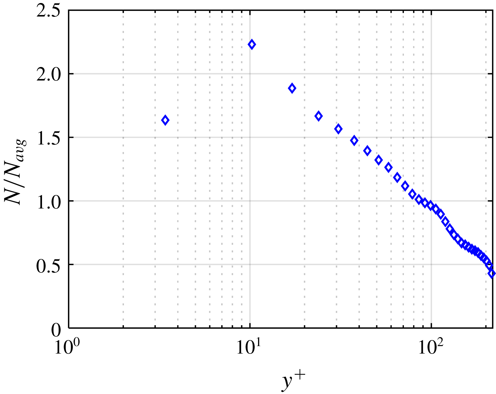
The distribution of the beads’ number density in the near-wall region is presented in figure 6. This distribution is determined based on the number of beads in each bin,
 $N$
, divided by the average number of beads across all the bins,
 $N_{avg}$
. The wall-normal location is normalized by
 $\unicode[STIX]{x1D706}$
. The averaging bin size for beads is equal to
 $d_{p}$
and the first data point is obtained at the centre of the first bin immediately after the wall (i.e. at
 $y^{+}=3.4$
). For this analysis, all the detected beads are considered, as no limitation is imposed on their trajectory length. As expected, the concentration of glass beads is higher close to the wall due to the gravity. The figure also demonstrates that local near-wall number density can be up to 2.2 times larger than the average number density within the measurement domain, i.e.
 $y^{+}<218$
region. The relatively small increase of local number density in the vicinity of the wall suggests that modulation of the liquid phase turbulence by the beads is small.
The normalized number density of glass beads in the near-wall region.

The velocity and acceleration statistics of glass beads obtained from the 3D-PTV measurement at
 $Re_{\unicode[STIX]{x1D70F}}=410$
are also investigated in this section. The velocity statistics are normalized using
 $u_{\unicode[STIX]{x1D70F}}$
, and the acceleration statistics are normalized using
 $u_{\unicode[STIX]{x1D70F}}^{3}/\unicode[STIX]{x1D710}$
. The
 $U^{+}$
profiles of beads and the unladen flow are compared in figure 7(a). The bead velocity is greater than that of the unladen flow at
 $y^{+}<10$
as the no-slip boundary condition does not apply to the beads. As a result,
 $\langle U_{f}\rangle -\langle U_{p}\rangle$
is negative; specifically, it is
 $-0.09~\text{m}~\text{s}^{-1}$
at
 $y^{+}=3.4$
which is approximately 10 % of the bulk velocity. At
 $y^{+}>10$
, the bead velocity is lower than that of the unladen flow. A similar observation was reported by Shao, Wu & Yu (Reference Shao, Wu and Yu2012) and Yu et al. (Reference Yu, Vinkovic and Buffat2016) and is associated with the larger inertia of beads (compared with that of the liquid phase). The trend of the
 $U^{+}$
profile is consistent with the results presented by others including Kussin & Sommerfeld (Reference Kussin and Sommerfeld2002), Shao et al. (Reference Shao, Wu and Yu2012) and Yu et al. (Reference Yu, Vinkovic and Buffat2016) for different values of
 $Re_{\unicode[STIX]{x1D70F}}$
and
 $St$
. The mean wall-normal velocity of unladen flow and glass beads is also normalized by
 $u_{\unicode[STIX]{x1D70F}}$
as
 $V^{+}=\langle V\rangle /u_{\unicode[STIX]{x1D70F}}$
, and presented in figure 7(b). The value of
 $V^{+}$
is close to zero for unladen flow in the whole measurement domain. However, glass beads have a small negative
 $V^{+}$
, showing their motion toward the lower wall. Therefore, the gravitational settling of beads is not totally balanced by turbulence diffusion. The former gradually accumulates the beads close to the wall, as seen in figure 6.
Comparison of 3D-PTV measurements of (a) mean streamwise velocity, (b) mean wall-normal velocity and (c) mean Reynolds stresses of beads (symbols) with the same parameters for the unladen flow (solid lines) at
 $Re_{\unicode[STIX]{x1D70F}}=410$
.

The normalized non-zero components of the Reynolds stress tensor of beads and the unladen flow are compared in figure 7(c), showing similar trends and approximately the same peak locations for the associated components. Beads have larger
 $\langle u^{2}\rangle$
in comparison with the unladen flow. Due to inertia, the glass beads can maintain their velocity for a longer time, and therefore over a longer wall-normal distance, relative to the fluid motions. As a result of this larger diffusion, a wider distribution of bead velocity, i.e. a larger velocity fluctuation, is observed (Shokri et al.
Reference Shokri, Ghaemi, Nobes and Sanders2017; Ahmadi et al.
Reference Ahmadi, Ebrahimian, Sanders and Ghaemi2019). The maximum of the absolute value of
 $\langle uv\rangle$
of beads,
 $|\langle uv\rangle |_{max}$
, is approximately 30 % larger than it is for the unladen flow, which indicates a greater correlation between their
 $u$
and
 $v$
and turbulence production. Shokri et al. (Reference Shokri, Ghaemi, Nobes and Sanders2017) compared the measured
 $\langle uv\rangle$
of inertial beads with unladen flow in an upward turbulent vertical pipe flow. Their results showed that the
 $|\langle uv\rangle |_{max}$
of beads (with
 $St^{+}$
values of 3.9 and 7.7) was approximately 30 % larger than the unladen flow. However, at
 $St^{+}=14$
,
 $|\langle uv\rangle |_{max}$
became 27 % smaller than
 $|\langle uv\rangle |_{max}$
for the unladen flow, indicating that the difference between
 $|\langle uv\rangle |_{max}$
of beads and unladen flow is strongly dependent on
 $St^{+}$
. The DNS results of Yu et al. (Reference Yu, Lin, Shao and Wang2017) showed a similar effect of
 $St$
on the difference between
 $|\langle uv\rangle |_{max}$
of particles and unladen flow in horizontal turbulent channel flows.
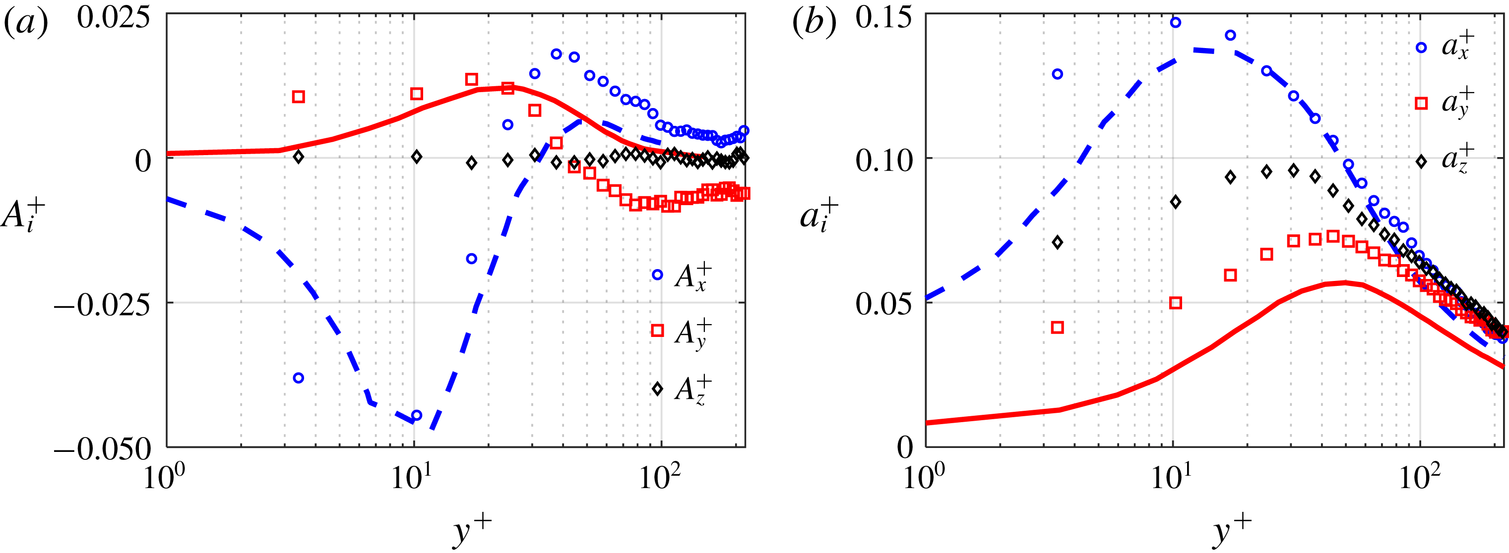
The normalized mean and r.m.s. of beads acceleration are compared with the numerical results of Zamansky et al. (Reference Zamansky, Vinkovic and Gorokhovski2011) in figure 8. This numerical simulation was carried out for small particles (
 $d_{p}^{+}<1$
) with a large density ratio (
 $r_{\unicode[STIX]{x1D70C}}=770$
). For this flow regime, Zamansky et al. (Reference Zamansky, Vinkovic and Gorokhovski2011) assumed point-particles, and the steady-state drag was the only force taken into account for the solid phase equations of motion. The effect of the added-mass, Basset, Saffman, Magnus and gravity forces were neglected. In the experiment,
 $d_{p}^{+}$
is larger and
 $r_{\unicode[STIX]{x1D70C}}$
is smaller. However, the numerical simulation is performed with
 $St^{+}=5$
and
 $Re_{\unicode[STIX]{x1D70F}}=587$
, which are close to the
 $St^{+}$
and
 $Re_{\unicode[STIX]{x1D70F}}$
of the current experiment. It should be noted that the comparison with the numerical simulation is not carried out here to evaluate the uncertainty of the 3D-PTV or the validity of the assumption for the numerical simulation. Here, we qualitatively compare the acceleration statistics of the experiment and the numerical simulation. The comparison also allows us to evaluate if the point-particle assumption is valid for the flow condition of the experiment. To the authors’ knowledge, this simulation is the best in comparison to the results of the current study, especially when one considers that mean and r.m.s. of acceleration are needed for the comparison.
From the
 $A_{x}^{+}$
profile of beads, presented in figure 8(a), bead deceleration (
 $A_{x}^{+}<0$
) occurs at
 $y^{+}<20$
with the minimum value of
 $A_{x}^{+}$
occurring at
 $y^{+}\approx 10$
. Bead deceleration is attributed to the slower viscous-dominated flow of the surrounding near-wall fluid and the interaction of beads with the wall. It is notable that the location of the minimum value of
 $A_{x}^{+}$
is close to the location of the minimum value of
 $\unicode[STIX]{x2202}\langle uv\rangle /\unicode[STIX]{x2202}y$
for beads shown in figure 7(c). Lavezzo et al. (Reference Lavezzo, Soldati, Gerashchenko, Warhaft and Collins2010) used DNS of a particle-laden flow, with
 $St_{K}=[0.87,1.76,11.8]$
to show that
 $\langle A_{x}\rangle$
and
 $\unicode[STIX]{x2202}\langle uv\rangle /\unicode[STIX]{x2202}y$
are related for inertial particles. The current experimental investigation also confirms this relation. The measured value at
 $y^{+}=3.4$
is
 $A_{x}^{+}=-0.038$
, while the numerical result at this location is
 $A_{x}^{+}=-0.019$
. This difference cannot be due to the different values of
 $St^{+}$
for as shown by Zamansky et al. (Reference Zamansky, Vinkovic and Gorokhovski2011), increasing
 $St^{+}$
from 1 to 5 does not considerably affect
 $A_{x}^{+}$
at this near-wall position. It also is not expected that the higher value of
 $Re_{\unicode[STIX]{x1D70F}}$
in the numerical study compared with the measurement is the reason for the difference in
 $A_{x}^{+}$
at
 $y^{+}=3.4$
. Yeo et al. (Reference Yeo, Kim and Lee2010) showed that increasing
 $Re_{\unicode[STIX]{x1D70F}}$
enhances the viscous force contribution and increases the deceleration; but this increment is negligible for
 $Re_{\unicode[STIX]{x1D70F}}>400$
. The difference between the measured
 $A_{x}^{+}$
and the numerical result at
 $y^{+}=3.4$
is attributed to the larger particles, smaller
 $r_{\unicode[STIX]{x1D70C}}$
and the bead–wall collision in the experiment. In the present study, the location of
 $A_{x}^{+}=0$
for beads is at
 $y^{+}\approx 20$
, which is closer to the wall than was found by Zamansky et al. (Reference Zamansky, Vinkovic and Gorokhovski2011). Comparison of the
 $A_{x}^{+}$
profiles for the solid-phase (figure 8
a) and the unladen flow (figure 5
a) shows that the two are different when
 $y^{+}>20$
: the unladen profile is relatively constant at a small positive value while for beads there is a local maximum at
 $y^{+}\approx 40$
, just above the buffer layer where
 $\unicode[STIX]{x2202}\langle uv\rangle /\unicode[STIX]{x2202}y$
is also positive, as shown in figure 7(c). The difference is mainly associated with the acceleration of the beads that are ejected away from the wall. The region of positive
 $A_{x}^{+}$
overlaps with the logarithmic layer and indicates where fluid applies a net positive force on the particles to accelerate them. The streamwise velocity difference between glass beads and fluid results in a drag force (Crowe et al.
Reference Crowe, Schwarzkopf, Sommerfeld and Tsuji2012), which causes a local maximum of
 $A_{x}^{+}$
at
 $y^{+}\approx 40$
.
Comparison between measurement of normalized (a) mean acceleration and (b) r.m.s. of acceleration components from the 3D-PTV (symbols) with the numerical results of Zamansky et al. (Reference Zamansky, Vinkovic and Gorokhovski2011) at
 $Re_{\unicode[STIX]{x1D70F}}=587$
with
 $St^{+}=5$
(lines).

The maximum value of
 $A_{y}^{+}$
is found at
 $y^{+}\approx 18$
of figure 8(a). This is the same location of the maximum value of
 $\unicode[STIX]{x2202}\langle v^{2}\rangle /\unicode[STIX]{x2202}y$
, as shown in figure 7(c), as well as the location of the maximum
 $A_{y}^{+}$
for the unladen flow, as shown in figure 5(a). This location is also near the mean axis of rotation of quasi-streamwise vortices, which is found at approximately
 $y^{+}\approx 20$
(Kim et al.
Reference Kim, Moin and Moser1987) where a minimum pressure is expected. The positive acceleration can be associated with the ejection motions of the fluid, which lift up the beads and transport them away from the wall (Kiger & Pan Reference Kiger and Pan2002). For particles moving toward the wall, their
 $V$
should decrease to result in a positive
 $A_{y}^{+}$
. In the region
 $18<y^{+}<40$
,
 $A_{y}^{+}$
decreases and becomes zero at
 $y^{+}\approx 40$
. Figure 8(a) shows that at
 $y^{+}<20$
, the
 $A_{y}^{+}$
of beads is larger than the
 $A_{y}^{+}$
reported by Zamansky et al. (Reference Zamansky, Vinkovic and Gorokhovski2011). After the zero
 $A_{y}^{+}$
point, the effect of gravity becomes dominant and the
 $A_{y}^{+}$
of beads becomes negative. The negative
 $A_{y}^{+}$
values were not observed in the numerical results of Zamansky et al. (Reference Zamansky, Vinkovic and Gorokhovski2011) in which gravity was not considered. As expected, the
 $A_{z}^{+}$
of glass beads is almost zero in the whole measurement domain. The maximum deviation of
 $A_{z}^{+}$
from zero is approximately
 $8.5\times 10^{-4}$
at
 $y^{+}=17$
.
Considering the r.m.s. of the bead acceleration in figure 8(b), the maximum value of
 $a_{x}^{+}$
of beads coincides with the location of the minimum value of
 $A_{x}^{+}$
in figure 8(a). The maximum value of
 $a_{x}^{+}$
is larger than those of Zamansky et al. (Reference Zamansky, Vinkovic and Gorokhovski2011). For unladen flow, Yeo et al. (Reference Yeo, Kim and Lee2010) observed that as
 $Re_{\unicode[STIX]{x1D70F}}$
increases from 408 to 600, the maximum value of
 $a_{x}^{+}$
increases by 3 %. The numerical results of Zamansky et al. (Reference Zamansky, Vinkovic and Gorokhovski2011) showed that the relationship between
 $St^{+}$
and
 $a_{x}^{+}$
is not monotonic:
 $a_{x}^{+}$
increased with increasing
 $St^{+}$
from 1 to 5, but decreased with further increases in
 $St^{+}$
. The greater values of
 $a_{x}^{+}$
at
 $St^{+}\sim 5$
compared to its values at the other
 $St^{+}$
in their simulations is associated with the balance between the particles’ response to the surrounding fluid and their wall-normal dispersion. The wall-normal dispersion is expected to initially increase with increasing
 $St^{+}$
, which results in acceleration/deceleration of beads when transported to different fluid layers, thereby increasing
 $a_{x}^{+}$
. The maximum value of
 $a_{y}^{+}$
in the measurement is also greater than that of the simulation. Again, the difference between
 $a_{x}^{+}$
and
 $a_{y}^{+}$
of the current measurement and those reported by Zamansky et al. (Reference Zamansky, Vinkovic and Gorokhovski2011) in the immediate vicinity of the wall is mainly associated with the larger particles and the smaller
 $r_{\unicode[STIX]{x1D70C}}$
in the experiment. The discrepancy suggests that the point-particle assumption cannot be applied to the conditions of the current experiment. The fully elastic particle–wall collision assumption applied in the numerical simulation and measurement noise can also contribute to the discrepancy in bead’s acceleration r.m.s. in the immediate vicinity of the wall.
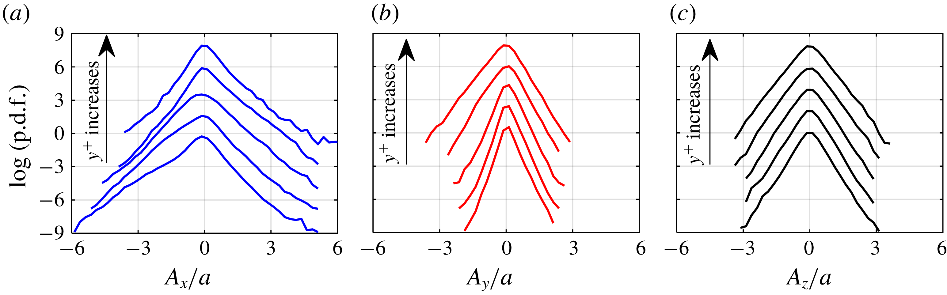
The probability density functions of the components of the bead mean acceleration normalized with the r.m.s. of total acceleration,
 $a$
, taken at five different
 $y^{+}$
, are presented in figure 9. As figure 9(a) shows, at
 $y^{+}=3.4$
and 10.2, the p.d.f. of
 $A_{x}$
is skewed towards negative
 $A_{x}$
, which is consistent with the results of figure 8(a) and the p.d.f.s produced from the measurements of Gerashchenko et al. (Reference Gerashchenko, Sharp, Neuscamman and Warhaft2008). It is conjectured that the negative skewness of the p.d.f. is due to the deceleration of beads by strong near-wall viscous forces and the beads’ interaction with the wall. With increasing
 $y^{+}$
, the viscous dominated deceleration reduces, and beads accelerate due to inertial forces. At
 $y^{+}=17$
, the p.d.f. is more symmetric. With further increases in
 $y^{+}$
to 44.3 and 98.8, the p.d.f. becomes right-skewed, which shows more beads tend to have positive
 $A_{x}$
.
Probability density functions of mean (a) streamwise, (b) wall-normal and (c) spanwise acceleration of beads. The curves in each plot, from bottom to top, correspond to
 $y^{+}=3.4$
, 10.2, 17, 44.3, 98.8. The p.d.f.s are each shifted up by two units of the vertical axis for clarity.

The p.d.f. of
 $A_{y}$
shown in figure 9(b) has a different behaviour than was described above for
 $A_{x}$
. Close to the wall and up to
 $y^{+}=44.3$
the p.d.f. is skewed right, indicating that more beads tend to have a positive
 $A_{y}$
, which means the value of
 $V$
of upward moving beads increases or the value of
 $V$
of downward moving beads decreases. The positive
 $A_{y}$
can be associated with several forces. As it was mentioned, ejection motions of the liquid phase are known to lift up and accelerate beads away from the wall (Kiger & Pan Reference Kiger and Pan2002). It is conjectured that the negative wall-normal pressure gradient also contributes to the positive
 $A_{y}$
of the upward moving beads. This pressure gradient has been attributed to a region of high vorticity where there is a larger accumulation of quasi-streamwise vortex cores located (Kim Reference Kim1989; Yeo et al.
Reference Yeo, Kim and Lee2010). In the high-shear near-wall region, glass beads can also experience a large Magnus force. For a downward moving bead, the value of
 $V$
is hypothesized to decrease due to the wall-normal pressure gradient and the increasing pressure of the fluid layer between the bead and the wall, known as wall repulsive force (Feng et al.
Reference Feng, Hu and Joseph1994). By increasing
 $y^{+}$
, the effect of these forces reduces, and glass beads experience a negative acceleration due to gravity. At
 $y^{+}>44.3$
, the
 $A_{y}$
p.d.f. is skewed to the negative side, indicating that a large number of the beads with upward motion slow down, and downward moving beads speed up under the effect of gravity. The p.d.f. of spanwise acceleration in figure 9(c) is symmetric as expected.
5 Quadrant analysis
The turbulent motion of the fluid and beads can be further analysed by plotting
 $u$
and
 $v$
in a quadrant plot. The motions described by the four quadrants are: Quadrant 1 (
 $Q_{1}$
), upward interactions with
 $u>0$
and
 $v>0$
; ejections (
 $Q_{2}$
) with
 $u<0$
and
 $v>0$
; downward interactions (
 $Q_{3}$
) with
 $u<0$
and
 $v<0$
; and sweeps (
 $Q_{4}$
) with
 $u>0$
and
 $v<0$
, as originally proposed by Wallace, Eckelmann & Brodkey (Reference Wallace, Eckelmann and Brodkey1972). To evaluate the contribution of each quadrant to
 $\langle uv\rangle$
, the motions of the unladen flow and beads are sampled based on the
 $u$
and
 $v$
signs of each quadrant. The conditionally sampled data are averaged as indicated by
 $\langle uv\rangle _{Q_{i}}$
, where
 $i$
varies from 1 to 4, referring to the four
 $u$
–
 $v$
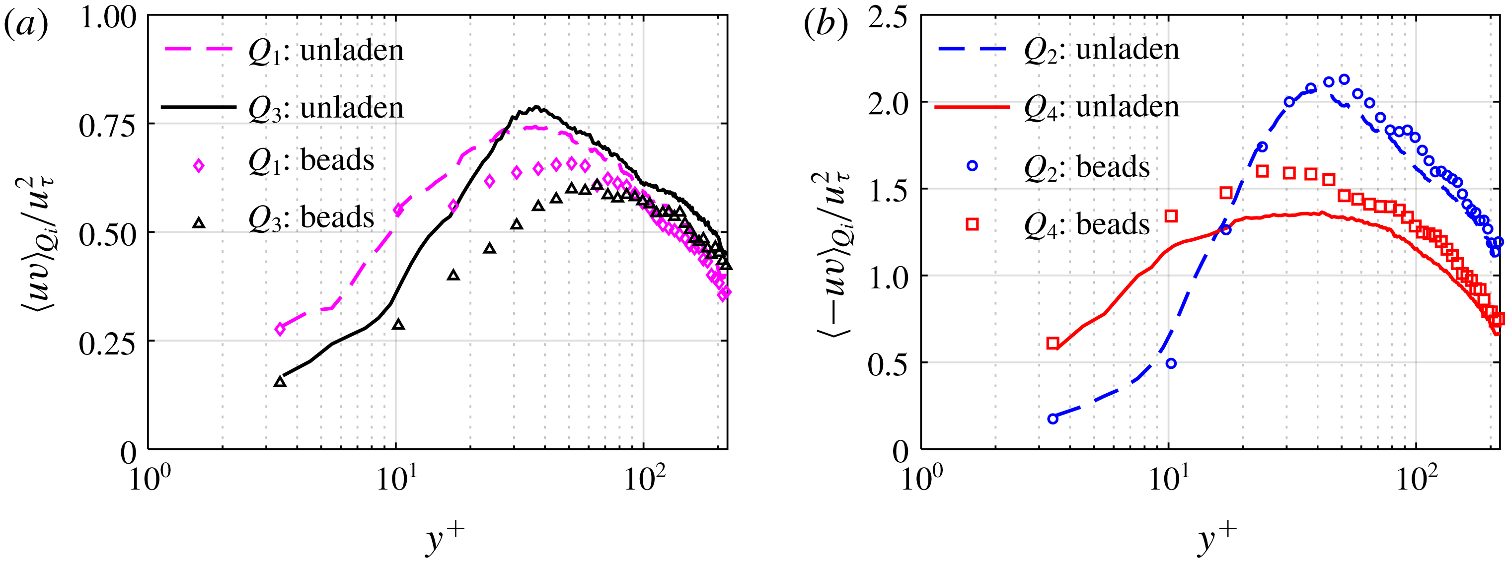
quadrants. Figure 10(a) shows the contribution of
 $Q_{1}$
and
 $Q_{3}$
while figure 10(b) shows the contribution of
 $Q_{2}$
and
 $Q_{4}$
. Based on the sign of
 $\langle uv\rangle$
and the positive
 $\unicode[STIX]{x2202}\langle U\rangle /\unicode[STIX]{x2202}y$
on the lower wall of the channel, the motions in
 $Q_{1}$
and
 $Q_{3}$
are associated with reduction of turbulence while motions represented in
 $Q_{2}$
and
 $Q_{4}$
generate turbulence. Comparison of figure 10(a) with figure 10(b) shows that there is poorer correlation of
 $u$
and
 $v$
for the beads in
 $Q_{1}$
and
 $Q_{3}$
than observed for the unladen flow; however, the beads with ejection and sweep motions in
 $Q_{2}$
and
 $Q_{4}$
have higher
 $\langle -uv\rangle$
compared with the unladen flow. Therefore, beads have a larger
 $\langle uv\rangle$
in the near-wall region which is consistent with their
 $\langle uv\rangle$
profile in figure 7(c). For the unladen flow, the sweep motion contributes more to turbulence production than ejection motions at
 $y^{+}<15$
. Farther from the wall at
 $y^{+}>15$
, the ejections become dominant as also observed in the DNS results of Kim et al. (Reference Kim, Moin and Moser1987). The beads with sweep and ejection motions also show a similar trend with the transition between sweep and ejection regions at
 $y^{+}=20$
.
Conditional average of Reynolds shear stress of the unladen flow and beads based on motions in the (a) first and third, and (b) second and fourth
 $u$
–
 $v$
quadrants.

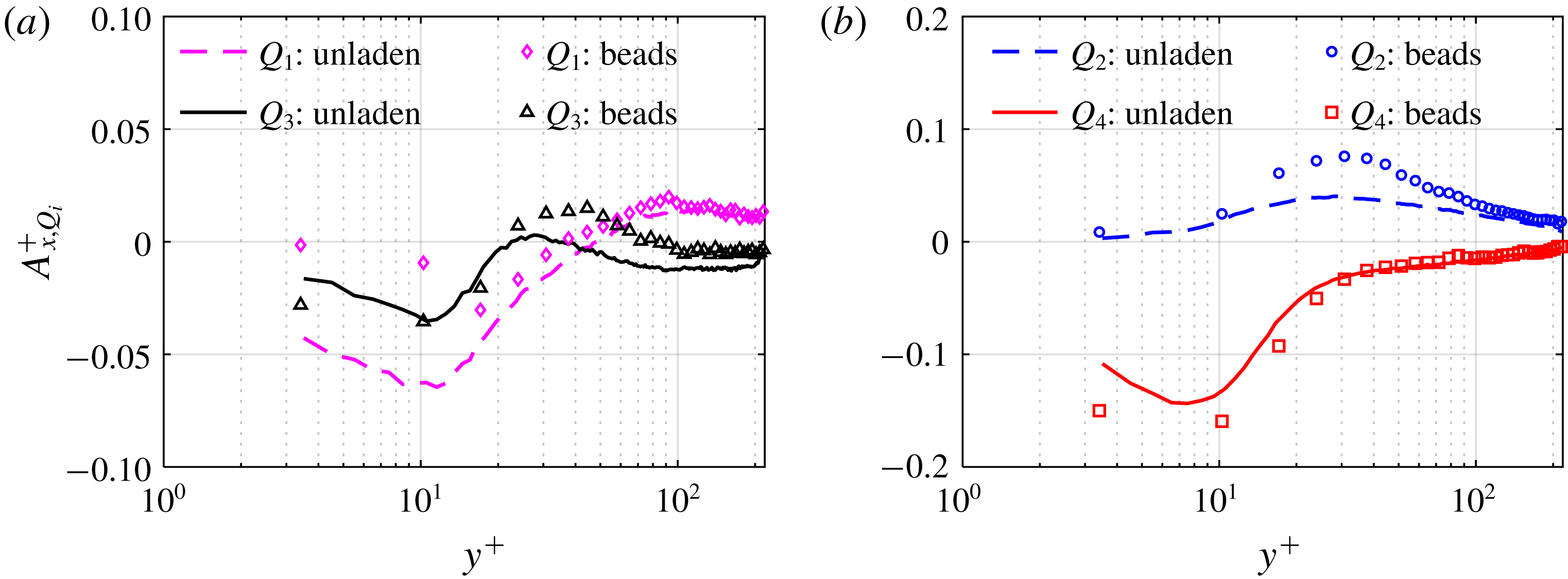
The quadrant analysis is extended in figure 11 to conditionally averaged acceleration,
 $A_{x,Qi}^{+}$
, of the unladen flow and beads to identify the contribution of quadrant motions to
 $A_{x}^{+}$
. The beads with
 $v>0$
(
 $Q_{1}$
and
 $Q_{2}$
) gain momentum from the high-speed region by moving away from the wall and have
 $A_{x}^{+}>0$
, except for
 $Q_{1}$
at
 $y^{+}<40$
where the viscous forces are dominant. At
 $y^{+}<20$
, only ejection motions of
 $Q_{2}$
result in positive
 $A_{x}^{+}$
. The maximum of the conditionally averaged
 $A_{x}^{+}$
based on
 $Q_{2}$
for both the unladen flow and beads is almost at the outer boundary of the buffer layer, or
 $y^{+}\sim 30$
. At this location, the viscous effects diminish and the surrounding fluid accelerates the ejected fluid and beads. The larger wall-normal displacement of beads due to their inertia moves them farther into the high-speed region. This results in higher drag force on the ejected beads compared with the ejected fluid. Therefore, the positive
 $A_{x}^{+}$
of beads is larger than that of the fluid, as shown in figure 11(b). It is also seen in this figure that in the near-wall region, sweep motions have
 $A_{x}^{+}<0$
for both the unladen flow and beads. The conditionally averaged
 $A_{x}^{+}$
based on
 $Q_{4}$
for unladen flow has a minimum at
 $y^{+}\approx 8$
while the minimum for beads is found at
 $y^{+}\approx 10$
. The locations of the minimum values of these conditional averages are consistent with the locations of the minimum values of
 $A_{x}^{+}$
shown in figure 5(a) and figure 8(a), respectively. Comparison of figures 11(a) and 11(b) shows that for both the unladen flow and beads, ejections and sweeps (
 $Q_{2}$
and
 $Q_{4}$
quadrants) are the major turbulent motions which provide positive and negative
 $A_{x}^{+}$
, respectively.
Conditional average of
 $A_{x}^{+}$
based on the motions in (a) first and third quadrants, and (b) second and fourth quadrants.

The conditionally averaged
 $A_{y}^{+}$
values, based again on
 $u$
–
 $v$
quadrant analysis, are shown in figure 12 for the unladen and bead-laden flows. As this figure shows, the positive
 $A_{y}^{+}$
of unladen flow is due to fluid elements with
 $v>0$
(
 $Q_{1}$
and
 $Q_{2}$
) in the whole near-wall region as well as sweep motions (
 $Q_{4}$
) at
 $y^{+}<100$
. The wall-normal pressure gradient induced by the low-pressure cores of the quasi-streamwise vortices pulls the flow upward and provides
 $A_{y}^{+}>0$
. At
 $y^{+}<100$
for the unladen flow it is only the motions in
 $Q_{3}$
that have negative contribution to
 $A_{y}^{+}$
. Similar trends are observed for beads but the values of
 $A_{y}^{+}$
are smaller because of gravity and their larger inertia compared with the unladen fluid flow. The
 $Q_{2}$
and
 $Q_{4}$
profiles for beads show that ejection and sweep motions have similar contribution to
 $A_{y}^{+}$
for the near-wall region: they both have
 $A_{y}^{+}>0$
at
 $y^{+}<40$
and
 $A_{y}^{+}<0$
at
 $y^{+}>40$
. Figure 12 shows that for both unladen flow and beads,
 $Q_{1}$
and
 $Q_{3}$
have the major contributions to positive and negative
 $A_{y}^{+}$
, respectively.
Conditional average of
 $A_{y}^{+}$
based on the motions in the (a) first and third quadrants, and (b) second and fourth quadrants.

6 Bead–wall interactions
In this section, the effect of the wall is analysed on beads with a wall separation distance of
 $y_{p}<d_{p}$
, where
 $y_{p}$
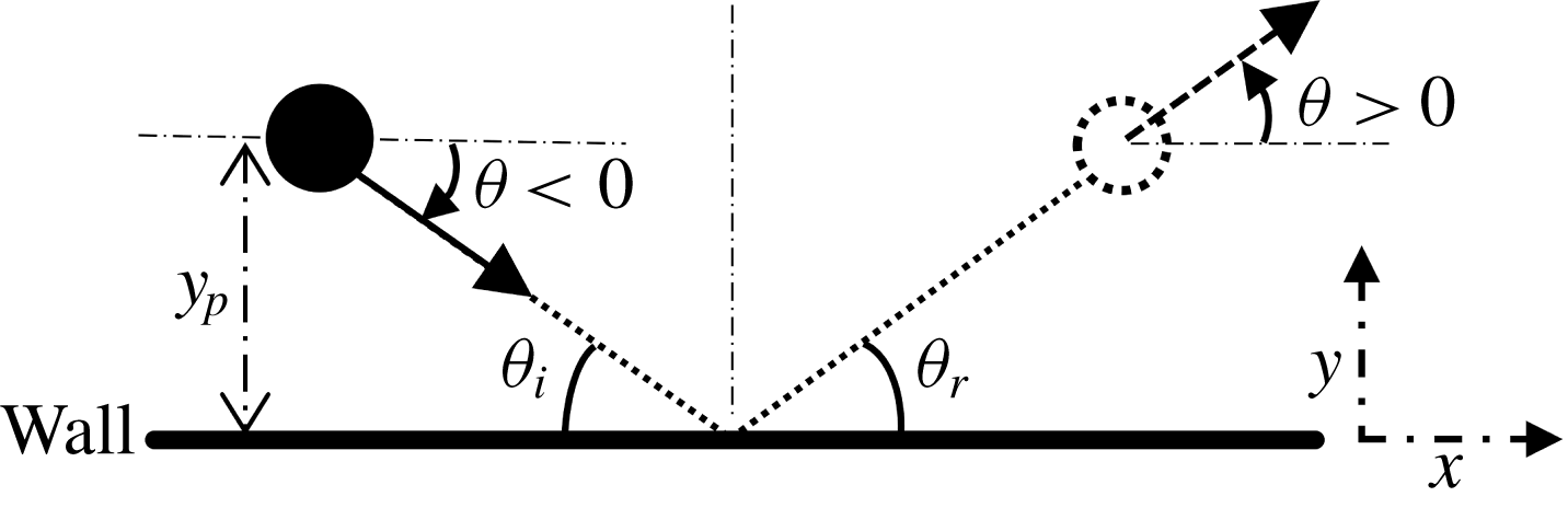
is the distance between the bead centre and the wall. The trajectory, velocity and acceleration of these near-wall beads is investigated. In addition, the temporal scales of the near-wall trajectories and their collision with the wall is statistically characterized. The bead trajectories are analysed based on the trajectory angle,
 $\unicode[STIX]{x1D703}$
, which is defined as
 $\tan ^{-1}(V/U)$
. Based on this definition and as seen in figure 13, a bead which is approaching the wall (i.e.
 $V<0$
) has a negative
 $\unicode[STIX]{x1D703}$
and a bead which is moving away from the wall (i.e.
 $V>0$
) has a positive
 $\unicode[STIX]{x1D703}$
. For a bead colliding with the lower wall of the channel, the impact angle,
 $\unicode[STIX]{x1D703}_{i}$
, and rebound angle,
 $\unicode[STIX]{x1D703}_{r}$
, are defined as the trajectory angle of the bead before and after collision, respectively. In total, more than 80 000 bead trajectories at
 $y_{p}<d_{p}$
were detected from 5 s of time-resolved 3D-PTV data.
A schematic to define the parameters used to characterize bead collision with the lower wall of the channel.

6.1 Trajectory angle
To scrutinize the relation of
 $\unicode[STIX]{x1D703}$
with velocity fluctuations for the beads at
 $y_{p}<d_{p}$
, the joint probability density function (j.p.d.f.) of
 $\unicode[STIX]{x1D703}$
and
 $u/u_{\unicode[STIX]{x1D70F}}$
, and the j.p.d.f. of
 $\unicode[STIX]{x1D703}$
and
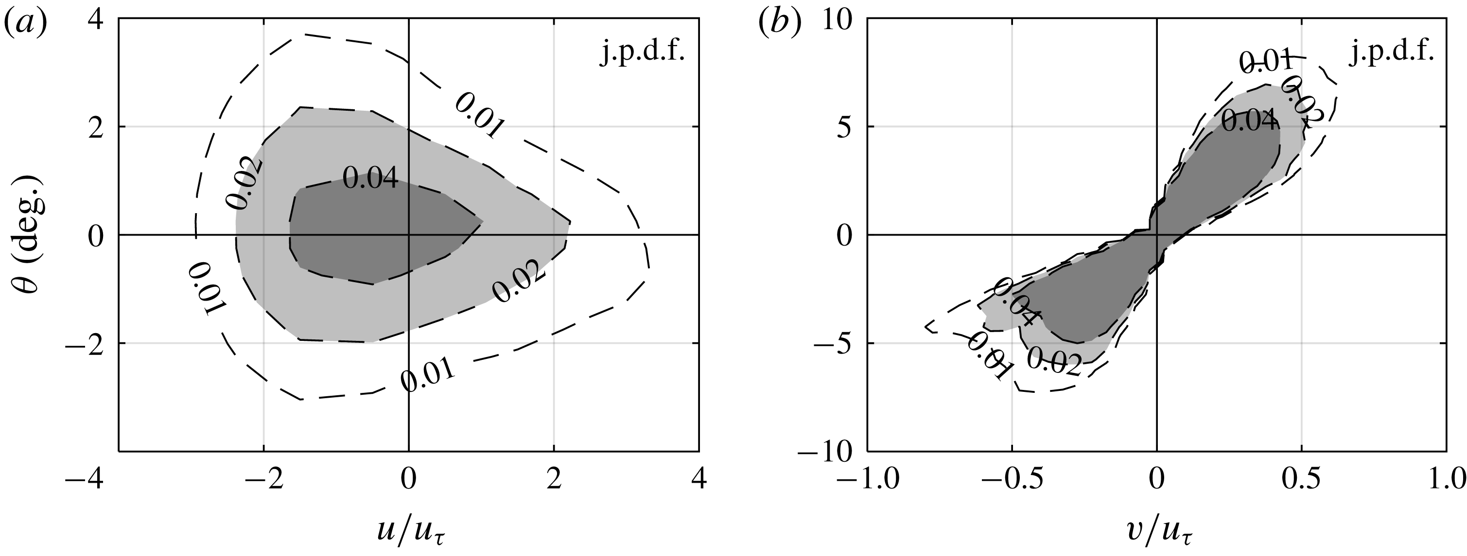
 $v/u_{\unicode[STIX]{x1D70F}}$
are shown in figures 14(a) and 14(b), respectively. The j.p.d.f. has a drop-shaped contour with a large variation of
 $\unicode[STIX]{x1D703}$
for large negative
 $u$
, and a small variation of
 $\unicode[STIX]{x1D703}$
for large positive
 $u$
. Therefore, the smaller is the instantaneous streamwise velocity of the bead,
 $U$
, the wider is the distribution of
 $\unicode[STIX]{x1D703}$
. This relation is pronounced here, since the mean streamwise velocity,
 $\langle U\rangle$
, is small in the vicinity of the wall. The relation between
 $\unicode[STIX]{x1D703}$
and
 $v$
is as expected; a positive
 $v$
results in a positive
 $\unicode[STIX]{x1D703}$
, and vice versa. It is also observed that distribution of
 $\unicode[STIX]{x1D703}$
becomes wider with increasing
 $v$
.
Joint probability density function of (a)
 $u/u_{\unicode[STIX]{x1D70F}}$
and
 $\unicode[STIX]{x1D703}$
, and (b)
 $v/u_{\unicode[STIX]{x1D70F}}$
and
 $\unicode[STIX]{x1D703}$
, for beads with
 $y_{p}<d_{p}$
.

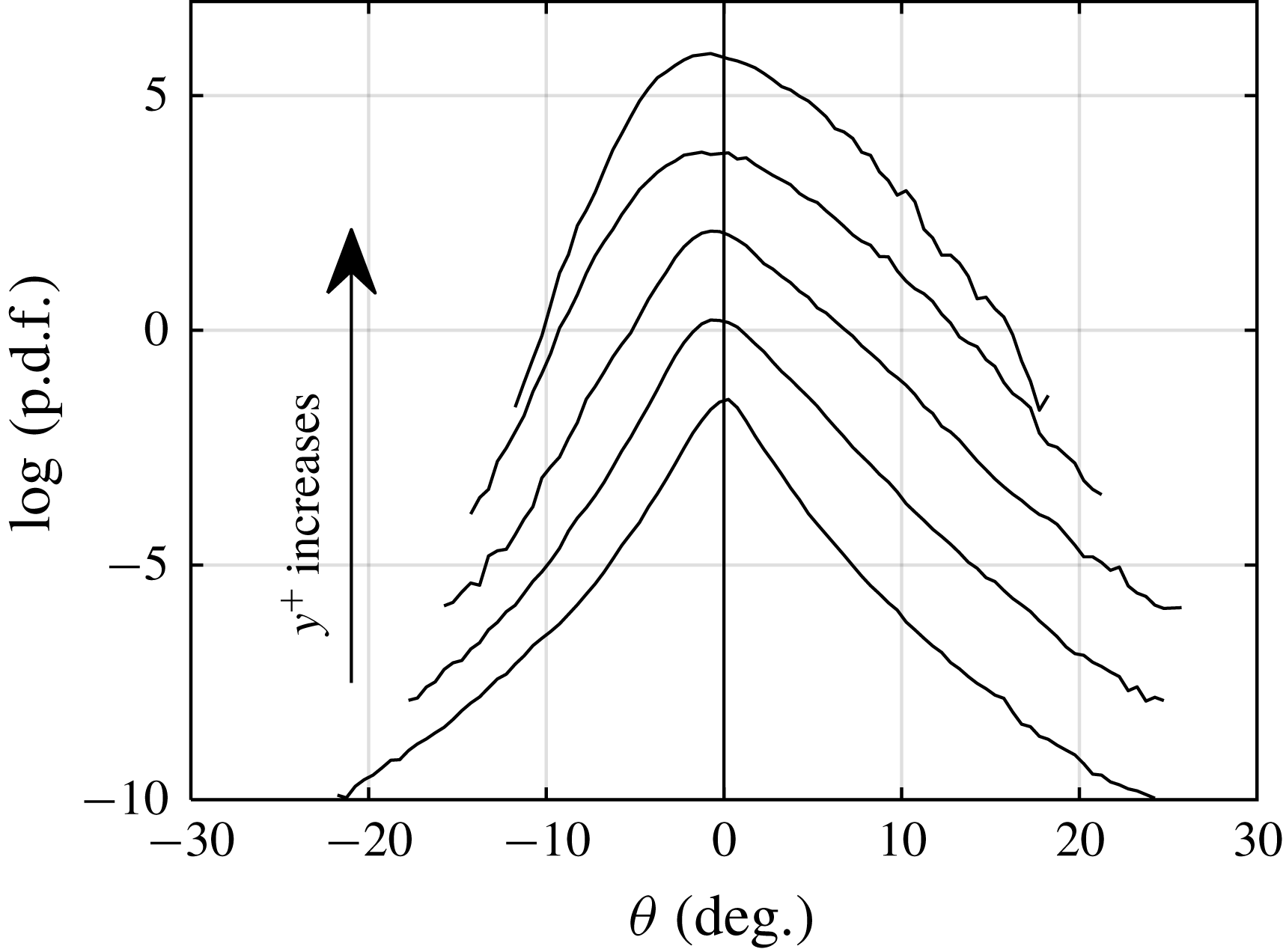
The p.d.f. of
 $\unicode[STIX]{x1D703}$
for beads in the vicinity of the wall at
 $y_{p}<d_{p}$
, i.e.
 $y^{+}=3.4$
, and higher
 $y^{+}$
locations, is shown in figure 15. The p.d.f. for
 $y^{+}=3.4$
has a larger peak at
 $\unicode[STIX]{x1D703}=0$
, while the tails of the p.d.f. extend to large positive and negative
 $\unicode[STIX]{x1D703}$
, reaching
 $\pm 20^{\circ }$
. This peaky behaviour of the p.d.f. reduces with increasing
 $y^{+}$
. At higher
 $y^{+}$
, the peak of the p.d.f. attenuates and shifts towards negative
 $\unicode[STIX]{x1D703}$
, which means that most of the trajectories descend toward the wall. It is also observed that the tail of the p.d.f. disappears with increasing
 $y^{+}$
as the probability of large
 $\unicode[STIX]{x1D703}$
becomes negligible. Therefore, the larger
 $\unicode[STIX]{x1D703}$
events are limited to the vicinity of the wall where the instantaneous streamwise velocity of the beads is small.
The p.d.f. of
 $\unicode[STIX]{x1D703}$
for beads at
 $y^{+}=3.4$
, 10.2, 17.0, 44.3 and 98.8, from bottom to top, respectively. The p.d.f.s are shifted up by two units of the vertical axis for clarity.

6.2 Velocity and acceleration
Conditional averaging is applied here to investigate the contribution of each quadrant of velocity fluctuations to instantaneous velocity and acceleration of the near-wall beads, i.e.
 $y_{p}<d_{p}$
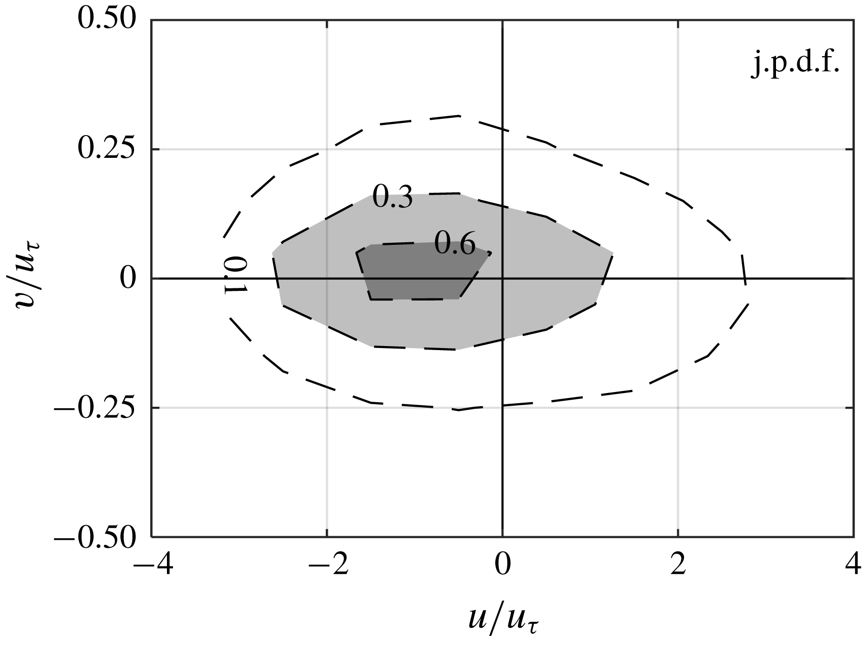
. First, to characterize the distribution of the motions, j.p.d.f. of
 $u$
and
 $v$
fluctuations of the beads is presented in figure 16. The j.p.d.f. is relatively symmetric with respect to the horizontal axis (
 $v=0$
). Most of beads have
 $u<0$
caused by (i) the fluid viscous force, as the surrounding fluid has lower velocity than beads and (ii) bead–wall interactions. The contours are also slightly shifted toward
 $v>0$
and more beads are in the second quadrant (
 $Q_{2}$
) than in the third quadrant (
 $Q_{3}$
). Considering the smaller
 $U$
of the fluid than the beads due to the no-slip boundary condition at
 $y^{+}=3.4$
, the Saffman force at this location should be downward. Therefore, it is the ejection motions, Magnus lift force, and wall collision, which can move the beads away from the wall and cause
 $v>0$
.
Joint probability density function of normalized velocity fluctuations. Only the beads with
 $y_{p}<d_{p}$
are considered.

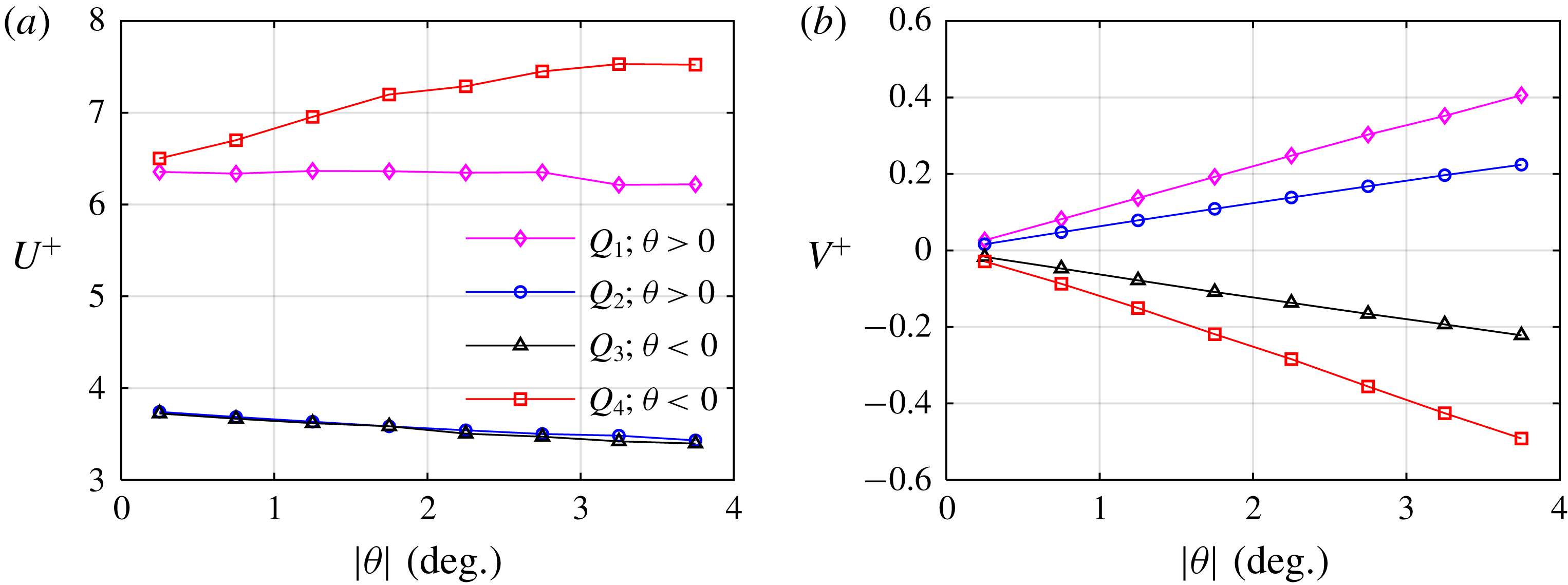
The relation between instantaneous velocity and the absolute value of trajectory angle,
 $|\unicode[STIX]{x1D703}|$
, is shown in figures 17(a) and 17(b) for the streamwise and wall-normal components, respectively. Results are also conditionally averaged based on the
 $u$
–
 $v$
quadrants of bead’s motion. The conditional averaging is carried out for
 $|\unicode[STIX]{x1D703}|<4^{\circ }$
with a bin size of
 $0.5^{\circ }$
. The
 $|\unicode[STIX]{x1D703}|<4^{\circ }$
range is applied to ensure statistical convergence as there are few beads outside this range. As expected, the beads with
 $Q_{1}$
and
 $Q_{4}$
motion (
 $u>0$
) have larger
 $U^{+}$
than the beads with
 $Q_{2}$
and
 $Q_{3}$
motion (
 $u<0$
) in figure 17(a). The
 $U^{+}$
of the beads in the first quadrant (
 $Q_{1}$
) is
 ${\sim}6.3u_{\unicode[STIX]{x1D70F}}$
and does not considerably change with
 $|\unicode[STIX]{x1D703}|$
; streamwise velocity of the beads with
 $Q_{1}$
motion is not a function of the trajectory angle. For the beads with a sweep motion (
 $Q_{4}$
),
 $U^{+}$
increases with increasing
 $|\unicode[STIX]{x1D703}|$
and reaches
 ${\sim}7.5u_{\unicode[STIX]{x1D70F}}$
at
 $|\unicode[STIX]{x1D703}|=4^{\circ }$
. This is because the beads with larger
 $|\unicode[STIX]{x1D703}|$
have come down from a higher
 $y^{+}$
, and therefore have higher
 $U^{+}$
. The
 $U^{+}$
value of the beads in
 $Q_{2}$
and
 $Q_{3}$
are almost equal at different
 $|\unicode[STIX]{x1D703}|$
, and for both quadrants,
 $U^{+}$
slightly decreases with increasing
 $|\unicode[STIX]{x1D703}|$
. As seen in figure 17(b), there is a linear relation between
 $|\unicode[STIX]{x1D703}|$
and
 $V^{+}$
, which indicates that
 $|\unicode[STIX]{x1D703}|$
is mainly caused by a variation of
 $V$
and not
 $U$
. The conditionally averaged values of
 $V^{+}$
also show that the beads with
 $Q_{1}$
and
 $Q_{4}$
motions (
 $u>0$
) have a larger magnitude of
 $V^{+}$
compared with the beads with
 $Q_{2}$
and
 $Q_{3}$
(
 $u<0$
). This means the faster beads (
 $Q_{1}$
and
 $Q_{4}$
) have a larger wall-normal velocity, which diffuses their momentum in the wall-normal direction.
Conditionally averaged (a)
 $U^{+}$
and (b)
 $V^{+}$
of beads based on
 $u$
–
 $v$
quadrants as functions of
 $|\unicode[STIX]{x1D703}|$
. Only the beads with
 $y_{p}<d_{p}$
are considered in this analysis.

The variation of conditionally averaged
 $A_{x}^{+}$
with
 $|\unicode[STIX]{x1D703}|$
is shown in figure 18(a) to compare the contributions of different quadrants. It is expected that the beads with upward motion (
 $Q_{1}$
and
 $Q_{2}$
) accelerate in the streamwise direction as they move upward into the regions with higher
 $U$
values. However, figure 18(a) shows that such a trend is only valid for
 $|\unicode[STIX]{x1D703}|>1$
, when the motion away from the wall is large enough. When the bead’s ascent angle is smaller than
 $1^{\circ }$
,
 $A_{x}^{+}$
for
 $Q_{1}$
and
 $Q_{2}$
motions is negative. The beads in
 $Q_{3}$
have downward motion (
 $\unicode[STIX]{x1D703}<0$
) and
 $A_{x}^{+}<0$
. In all these cases, streamwise deceleration is associated with viscous deceleration by the near-wall fluid and particle–wall collisions. Figure 18(a) shows that beads with sweeping motion in the
 $Q_{4}$
quadrant experience the highest streamwise deceleration. The deceleration of these beads also increases with increasing
 $|\unicode[STIX]{x1D703}|$
. This larger deceleration of trajectories with large
 $|\unicode[STIX]{x1D703}|$
is associated with a larger viscous drag due to their greater velocity difference with respect to the surrounding fluid; the beads with larger
 $|\unicode[STIX]{x1D703}|$
have come down from higher
 $y^{+}$
locations with higher velocity.
Conditionally averaged (a)
 $A_{x}^{+}$
and (b)
 $A_{y}^{+}$
of beads based on
 $u$
–
 $v$
quadrants as functions of
 $|\unicode[STIX]{x1D703}|$
. Only the beads with
 $y_{p}<d_{p}$
are considered in this analysis.

The variation of conditionally averaged
 $A_{y}^{+}$
values is also investigated for the
 $u$
–
 $v$
quadrants and is presented in figure 18(b). All four quadrants have a positive
 $A_{y}^{+}$
. As it was explained previously, a positive
 $A_{y}^{+}$
indicates acceleration of upward moving beads and deceleration of downward moving beads. For the sweeping motion of
 $Q_{4}$
, a strong increase in
 $A_{y}^{+}$
with increasing
 $|\unicode[STIX]{x1D703}|$
is observed. The larger positive
 $A_{y}^{+}$
of the sweeping beads is attributed to greater wall-normal drag and wall repulsive force as they approach the wall under a larger
 $|\unicode[STIX]{x1D703}|$
. A strong increase in
 $A_{y}^{+}$
with increasing
 $|\unicode[STIX]{x1D703}|$
, is also observed for the upward moving beads (
 $v>0$
) in
 $Q_{1}$
. Therefore, upward trajectories with a larger angle undergo a stronger wall-normal acceleration. A possible cause of this trend can be stronger ejection events which accelerate the beads upward under a larger ascent angle. The
 $A_{y}^{+}$
of beads with
 $Q_{2}$
motion slightly increases with increasing
 $|\unicode[STIX]{x1D703}|$
, while the
 $A_{y}^{+}$
of beads in
 $Q_{3}$
does not show a strong and monotonic dependence on
 $|\unicode[STIX]{x1D703}|$
. In general, beads with
 $u>0$
(
 $Q_{1}$
and
 $Q_{4}$
) have greater
 $A_{y}^{+}$
than the beads with
 $u<0$
(
 $Q_{2}$
and
 $Q_{3}$
). As was seen in figure 17(b), the beads with
 $u>0$
have a larger
 $V^{+}$
, which can cause a larger velocity difference relative to the surrounding fluid. Therefore, a larger drag force can act on beads with
 $u>0$
, which increases their
 $A_{y}^{+}$
.
6.3 Temporal scales
The temporal autocorrelation of beads’ motion is investigated here to characterize their time scales at different wall-normal distances. For a variable
 $S$
, the autocorrelation coefficient is determined as
 $C_{SS}(t)=\langle S(t_{0}^{+})S(t_{0}^{+}+t^{+})\rangle /\langle S^{2}(t_{0})\rangle$
, where
 $S(t_{0}^{+})$
is the value of
 $S$
at the initial time step of
 $t_{0}^{+}$
, and
 $t^{+}$
is the time shift. This autocorrelation is calculated from the time-resolved values of
 $U$
,
 $V$
,
 $W$
and
 $\unicode[STIX]{x1D703}$
along the bead trajectories. The results are shown in figure 19 at five different
 $y^{+}$
. In general, all the autocorrelation coefficients decrease with increasing
 $t^{+}$
. The
 $C_{UU}$
coefficient indicates that streamwise velocity of the beads stays correlated for a longer time since
 $C_{UU}$
stays positive for a long
 $t^{+}$
, beyond the investigated range. However,
 $C_{VV}$
,
 $C_{WW}$
and
 $C_{\unicode[STIX]{x1D703}\unicode[STIX]{x1D703}}$
coefficients reach close to zero within
 $t^{+}<100$
for all the investigated
 $y^{+}$
.
Temporal autocorrelation of (a)
 $U$
, (b)
 $V$
, (c)
 $W$
and (d)
 $\unicode[STIX]{x1D703}$
of glass beads. The curves in each plot, from bottom to top, correspond to
 $y^{+}=3.4$
, 10.2, 17.0, 44.3 and 98.8.

The autocorrelation coefficients approach zero at a larger gradient with decreasing
 $y^{+}$
, which indicates a smaller time scale of the beads’ motion. This is expected as the turbulent structures of fluid phase also become smaller with decreasing
 $y^{+}$
. However, the
 $C_{VV}$
and
 $C_{\unicode[STIX]{x1D703}\unicode[STIX]{x1D703}}$
at
 $y^{+}=3.4$
demonstrate a different trend due to the presence of local minimums and negative values. At
 $y^{+}=3.4$
, with increasing
 $t^{+}$
, there is an initial and rapid decrease of
 $C_{VV}$
to a local minimum at
 $t^{+}=11$
. This is followed by a small increase and then a reduction to negative values at
 $t^{+}=20$
. For the same wall-normal location of
 $y^{+}=3.4$
,
 $C_{\unicode[STIX]{x1D703}\unicode[STIX]{x1D703}}$
rapidly decreases and reaches a local minimum also at
 $t^{+}=11$
. The time shift,
 $t^{+}$
, to reach negative
 $C_{VV}$
and
 $C_{\unicode[STIX]{x1D703}\unicode[STIX]{x1D703}}$
, both indicate the time scale when the bead changes its wall-normal direction of motion, shift from upward to downward motion, and vice versa. However, the local minimum is more pronounced for
 $C_{\unicode[STIX]{x1D703}\unicode[STIX]{x1D703}}$
since
 $\unicode[STIX]{x1D703}$
is strongly modulated by the small magnitude of
 $U$
according to
 $\unicode[STIX]{x1D703}=\tan ^{-1}(V/U)$
. Therefore, change in the direction of a weak wall-normal motion (small
 $V$
) can result in a significant change of
 $\unicode[STIX]{x1D703}$
if
 $U$
is small.
6.4 Collision with the wall
The momentum exchange of beads during bead–wall collision is investigated by analysing bead trajectories that are in a narrower wall separation distance relative to the previous analysis. In this analysis, only beads that the distance of their centroid from the wall is equal to, or smaller than, half of the mean particle diameter (i.e.
 $y_{p}\leqslant 0.5d_{p}$
) are considered. This resulted in approximately 34 000 bead trajectories within 5 s of time-resolved 3D-PTV data. For these near-wall trajectories, wall-collision is defined when the bead also has a negligible wall-normal velocity. This criterion is imposed when the instantaneous wall-normal bead velocity,
 $V$
, is an order of magnitude smaller than the average of the absolute wall-normal bead velocity,
 $\langle |V|\rangle$
. Therefore,
 $|V|<0.1\langle |V|\rangle$
, where
 $\langle |V|\rangle =0.01~\text{m}~\text{s}^{-1}$
at
 $y^{+}=3.4$
. The period when this criterion is valid is defined as the wall-interaction time,
 $t_{i}$
. For the tracks with a detected collision and within
 $y^{+}\leqslant 0.5d_{p}^{+}$
, the absolute value of trajectory angle before collision is averaged and indicated as
 $|\unicode[STIX]{x1D703}_{i}|$
. The average trajectory angle after collision is also estimated and denoted as the average rebound angle,
 $\langle \unicode[STIX]{x1D703}_{r}\rangle$
.
The variation of the estimated
 $\langle \unicode[STIX]{x1D703}_{r}\rangle$
with
 $|\unicode[STIX]{x1D703}_{i}|$
is presented in figure 20(a). For
 $|\unicode[STIX]{x1D703}_{i}|<1.5^{\circ }$
,
 $\langle \unicode[STIX]{x1D703}_{r}\rangle$
is greater than
 $|\unicode[STIX]{x1D703}_{i}|$
, meaning that trajectories with small
 $\unicode[STIX]{x1D703}$
rebound at a larger angle and disperse through collision with the wall. Beads with
 $|\unicode[STIX]{x1D703}_{i}|>1.5^{\circ }$
rebound at a smaller angle;
 $\langle \unicode[STIX]{x1D703}_{r}\rangle <|\unicode[STIX]{x1D703}_{i}|$
. The normalized average of the wall-interaction time (
 $t_{i}^{+}=\langle t_{i}\rangle /t_{f}$
) is presented in figure 20(b) as a function of
 $|\unicode[STIX]{x1D703}_{i}|$
. Inspection of the data shows that a bead with
 $|\unicode[STIX]{x1D703}_{i}|<1.5^{\circ }$
can spend on average
 $5t_{f}$
in contact with the wall. Such beads may have multiple small collisions with the wall or slide along it. The wall-interaction time scale approaches a constant value of approximately 1.6 for beads with
 $|\unicode[STIX]{x1D703}_{i}|>1.5^{\circ }$
.
(a) The average rebound angle and (b) the wall-interaction time scale of beads as a function of incident angle.

The average restitution ratio of beads (the ratio of the rebound velocity to the incident velocity) in the streamwise direction,
 $\langle e_{U}\rangle$
, and wall-normal,
 $\langle e_{V}\rangle$
, are determined and presented in figure 21 to show their variation with
 $|\unicode[STIX]{x1D703}_{i}|$
. Figure 21(a) shows that for small incident angles of
 $|\unicode[STIX]{x1D703}_{i}|<1^{\circ }$
,
 $\langle e_{U}\rangle$
is close to 1 which means that the sliding beads have negligible momentum exchange and undergo elastic collision in the streamwise direction. This is consistent with the smaller
 $A_{x}^{+}$
values observed for downward moving beads (
 $Q_{3}$
and
 $Q_{4}$
) at small
 $|\unicode[STIX]{x1D703}|$
, as seen in figure 18(a). As the incident angle becomes steeper (
 $|\unicode[STIX]{x1D703}_{i}|>1^{\circ }$
),
 $\langle e_{U}\rangle$
reduces to
 ${\sim}0.925$
for
 $|\unicode[STIX]{x1D703}_{i}|>2^{\circ }$
. In other words, the streamwise momentum of these beads reduces by 7.5 % due to collision with the wall.
Variation of (a) streamwise and (b) wall-normal bead restitution ratios with absolute incident angle.

The beads with
 $|\unicode[STIX]{x1D703}_{i}|<1.5^{\circ }$
have wall-normal restitution ratios,
 $\langle e_{V}\rangle$
, greater than 1 as seen in figure 21(b). These beads slide on the wall over a longer period of time as seen in figure 20(b). The longer interaction increases the angular velocity of a bead since the bottom surface of the bead is subject to surface friction due to the interaction with the wall, while its upper surface is subjected only to shear. This angular velocity is known to produce the Magnus lift force (Rubinow & Keller Reference Rubinow and Keller1961). The Magnus force in the wall-normal direction can be determined as
 $F_{mag}=\unicode[STIX]{x03C0}d_{p}^{3}\unicode[STIX]{x1D70C}_{f}\unicode[STIX]{x1D714}(U_{p}-U_{f})/8$
(Crowe et al.
Reference Crowe, Schwarzkopf, Sommerfeld and Tsuji2012). Here,
 $\unicode[STIX]{x1D714}$
is the angular velocity of a glass bead, which is approximated as the half of the local shear rate (Drew & Passman Reference Drew and Passman1999). Based on the unladen mean velocity profile, the mean shear rate at
 $y^{+}=3.4$
is approximately 2800
 $1~\text{s}^{-1}$
. At this wall-normal location,
 $\langle U_{p}\rangle -\langle U_{f}\rangle$
is approximately
 $0.09~\text{m}~\text{s}^{-1}$
. Therefore, the approximate
 $F_{mag}$
for a glass bead at
 $y^{+}=3.4$
is approximately
 $9.7\times 10^{-8}$
N. This force is approximately four times more than the weight of a glass bead (
 ${\sim}2.5\times 10^{-8}$
N) and can potentially lift a glass bead. This type of particle motion, where particle lift occurs after some period of sliding on the bottom wall, was observed in figure 3 and was also recently observed by Barros, Hiltbrand & Longmire (Reference Barros, Hiltbrand and Longmire2018). Based on these observations, the fact that
 $\langle e_{V}\rangle >1$
does not mean that the bead gains wall-normal momentum through collision with the wall; the excess momentum is due to the additional angular momentum which in turn produces a lift force. By increasing
 $|\unicode[STIX]{x1D703}_{i}|$
,
 $\langle e_{V}\rangle$
decreases to a value of approximately 0.8 for the beads with
 $|\unicode[STIX]{x1D703}_{i}|>1.75^{\circ }$
. Generally, increasing the incident angle increases the wall-normal momentum loss and results in lower values of
 $\langle e_{V}\rangle$
.
7 Summary and conclusions
To characterize acceleration statistics and wall-collision of inertial particles in non-isotropic near-wall turbulence, glass beads with
 $d_{p}^{+}=6.8$
at a volume concentration of 0.03 % in a turbulent channel flow at
 $Re_{\unicode[STIX]{x1D70F}}=410$
were investigated using time-resolved 3D-PTV. It has been shown that for glass beads, there are qualitative relations between the wall-normal variations of
 $\langle A_{x}\rangle$
and
 $\unicode[STIX]{x2202}\langle uv\rangle /\unicode[STIX]{x2202}y$
as well as
 $\langle A_{y}\rangle$
and
 $\unicode[STIX]{x2202}\langle v^{2}\rangle /\unicode[STIX]{x2202}y$
. Comparison of the wall-normal acceleration of glass beads and unladen flow showed similarities between bead dynamics and the near-wall fluid dynamics. The investigations show the presence of two layers based on the acceleration of the beads: (i) an inner layer in the vicinity of the wall at approximately
 $y^{+}<20$
, and (ii) an outer layer at farther distance from the wall at
 $y^{+}>20$
.
Within the inner-layer, the beads decelerated (on average) in the streamwise direction. The maximum negative streamwise deceleration was observed at
 $y^{+}=10$
and it gradually reduced to zero at
 $y^{+}=20$
. In the inner-layer, a large percentage of the beads had velocities less than the average bead velocity and their turbulent motions belonged to the second and the third quadrants of velocity fluctuations. However, the bead dynamics in this layer were dominated by the extreme motions of a smaller number of beads in the fourth quadrant. These beads had a sweeping motion toward the wall and demonstrated the largest streamwise momentum and deceleration. The wall-normal acceleration of the beads in the inner layer was positive, which indicated an increase in wall-normal velocity when a bead moves away from the wall, or a reduction of wall-normal velocity when a bead moves towards the wall.
In the outer layer, the beads had an overall positive streamwise acceleration, which peaked at approximately
 $y^{+}=30$
. The peak was associated with the beads in the second quadrant, i.e. an ejection motion. The maximum transfer of momentum from the liquid phase to the beads occurred in the logarithmic layer, where the streamwise acceleration of the beads was large and positive. However, the streamwise acceleration gradually attenuated with increasing
 $y^{+}$
. At a farther distance from the wall, the positive streamwise acceleration of the beads moving away from the wall was balanced by the negative streamwise acceleration of the beads moving towards the wall. The outer-layer beads also had a negative wall-normal acceleration, which was associated with an increase in the wall-normal velocity of beads in the third and fourth quadrant, and reduction in the wall-normal velocity of beads of the first and second quadrant.
The interaction of glass beads with the wall was studied by analysing the trajectory angle, velocity and acceleration of the beads found in the immediate vicinity of the wall. At
 $y_{p}<d_{p}$
, beads with sweeping motion had the maximum momentum, streamwise deceleration, and wall-normal acceleration compared with other beads. These terms increased with increasing the trajectory angle,
 $|\unicode[STIX]{x1D703}|$
. At
 $y_{p}=d_{p}/2$
, the bead trajectory angle had a peaky distribution; a large number of beads had a near zero angle while there were occasional extremely large trajectory angles of up to
 $20^{\circ }$
. The latter was associated with the near-wall beads that had a small streamwise velocity. With increasing
 $y^{+}$
, the trajectory angle did not demonstrate a peaky distribution, and the mode of the distribution was slightly negative as most of the beads gradually settled toward the wall. For beads within
 $y_{p}\leqslant d_{p}/2$
, wall collision was defined when a bead had a negligible wall-normal velocity. The beads with an incident angle of
 $|\unicode[STIX]{x1D703}_{i}|<1.5^{\circ }$
had a longer average interaction time with the wall, which could be as long as
 ${\sim}5t_{f}$
. These beads were referred to as the sliding beads and had a negligible streamwise momentum exchange (
 ${\sim}5\,\%$
) during their interaction with the wall. It is conjectured that their longer interaction time increased the effect of the Magnus lift force on them. As a result, their average rebound angle was larger than their incident angle and their wall-normal restitution coefficient was larger than one. The beads with sharper collision angle with the wall of
 $|\unicode[STIX]{x1D703}_{i}|>1.5^{\circ }$
had smaller streamwise and wall-normal restitution coefficients, and also a smaller average wall-interaction time. The autocorrelation coefficients of wall-normal velocity and trajectory angle had a local minimum with negative value at a time-shift of approximately
 $11t_{f}$
. This indicates the average time for change in the direction of wall-normal motions for the beads at
 $y_{p}\leqslant d_{p}/2$
due to their interaction with the wall. A negative autocorrelation coefficient was not observed for the beads at a farther distance from the wall.
In general, this experimental investigation shows that the assumptions of point-particles and elastic particle–wall collision are inadequate for accurate modelling of large inertial beads in water. The discrepancy between the acceleration profiles from the experiments and those from the numerical simulation of Zamansky et al. (Reference Zamansky, Vinkovic and Gorokhovski2011) showed that the point-particle assumption is not valid for large particles (
 $d_{p}^{+}=6.8$
) with small density relative to the carrier phase (
 $\unicode[STIX]{x1D70C}_{p}/\unicode[STIX]{x1D70C}_{f}=2.5$
). Measurements of particles’ velocity also showed evidence of prolonged interactions with the wall for particles that impact the wall at a shallow angle. This resulted in an increase of beads’ momentum, which cannot be accounted for using the steady-state drag of the point-particle model. In addition, the measurements demonstrated evidence of inelastic particle–wall collisions with considerable loss of momentum at larger impact angles.
Appendix A. Uncertainty evaluation
A quadratic regression is applied on each position component of the tracers and glass beads along their trajectory to reduce the noise and estimate their velocity and acceleration. A quadratic regression over a long period (i.e. large temporal kernel) can filter out the high-frequency content of the data while a short kernel may not be effective in reducing the noise. Therefore, the size of the temporal kernel of the quadratic fit is optimized by evaluating the minimum kernel length just before the increase in noise of acceleration r.m.s. following the method used by Gerashchenko et al. (Reference Gerashchenko, Sharp, Neuscamman and Warhaft2008). The variation of the normalized r.m.s. of streamwise acceleration,
 $a_{x}^{+}=a_{x}/(u_{\unicode[STIX]{x1D70F}}^{3}/\unicode[STIX]{x1D710})$
, of tracers with the temporal kernel size is evaluated in figure 22 at
 $y^{+}=3.4$
. It is observed that
 $a_{x}^{+}$
rapidly increases when the kernel size becomes smaller than 3 ms. The point where the variation of
 $a_{x}^{+}$
with reduction of the kernel size deviates from a straight line (more than 1 %) is selected as the appropriate temporal kernel size. This optimum kernel is estimated at
 $t=4.5$
ms in figure 22.
The dependence of streamwise acceleration r.m.s. of the tracers at
 $y^{+}=3.4$
on the temporal kernel of the quadratic regression fit. The dashed straight line shows the fitted line based on the method presented by Voth et al. (Reference Voth, La Porta, Crawford, Alexander and Bodenschatz2002). The extrapolation of
 $a_{x}^{+}$
to
 $t=0$
based on this fit is 0.155.

Voth et al. (Reference Voth, La Porta, Crawford, Alexander and Bodenschatz2002) showed that the acceleration r.m.s. can be estimated as a summation of an exponential term (represents the contribution of turbulence) and a power law term (represents the contribution of position noise). They argued that an estimation of the acceleration r.m.s. can be obtained by extrapolation of the exponential term to zero temporal kernel. They confirmed that this extrapolation overestimates the true value of acceleration variance by approximately 10 % based on comparison with the DNS results of Vedula & Yeung (Reference Vedula and Yeung1999). The extrapolation of the exponential term to
 $t=0$
in figure 22 results in
 $a_{x}^{+}=0.155$
which is approximately 13 % larger than the
 $a_{x}^{+}=0.137$
at
 $y^{+}=3.4$
obtained based on a kernel of 4.5 ms.
The performance of the quadratic regression in reducing the noise in estimating particle position is investigated by calculating the pre-multiplied linear spectral density (LSD) of the
 $x$
,
 $y$
and
 $z$
components of tracer trajectories before and after applying the polynomial regression, following the method of Gesemann et al. (Reference Gesemann, Huhn, Schanz and Schröder2016). The result is presented in figure 23 as a function of the frequency,
 $f$
, normalized by the Nyquist frequency,
 $f_{N}$
, for positional error in
 $x$
,
 $y$
and
 $z$
location of tracers. When no polynomial regression is applied, a flat section is observed in the high-frequency end of the LSD, which shows the measurement noise. Based on this flat section, the estimated noise level is approximately 6, 10 and
 $5~\unicode[STIX]{x03BC}\text{m}$
that is equivalent to 0.1, 0.2 and 0.1 pixel in
 $x$
,
 $y$
and
 $z$
directions, respectively. As expected, the out of plane component has a larger noise level. As seen in figure 23, the quadratic regression reduced the high-frequency random noise while it does not affect the low-frequency motions. The normalized cross-over frequency, the frequency at which the LSD profile after regression crosses the estimated noise level, is 0.49, 0.18 and 0.51 for the
 $x$
,
 $y$
and
 $z$
components, respectively.
Linear spectral density of (a)
 $x$
-, (b)
 $y$
- and (c)
 $z$
-components of tracers’ position in unladen flow with and without applying quadratic regression. The dashed-dotted lines show the measurement noise level in each component.

The difference between the measured velocity statistics of the unladen flow at
 $y^{+}=3.4$
with those from DNS of Moser et al. (Reference Moser, Kim and Mansour1999) at
 $Re_{\unicode[STIX]{x1D70F}}=395$
is presented in table 5. For acceleration statistics, the measured statistics of the unladen flow are compared with DNS of Yeo et al. (Reference Yeo, Kim and Lee2010) at
 $Re_{\unicode[STIX]{x1D70F}}=410$
. It should be noted that the difference between the velocity statistics of the present study and the DNS of Moser et al. (Reference Moser, Kim and Mansour1999) can be partially due to the small difference in
 $Re_{\unicode[STIX]{x1D70F}}$
.
An estimation of uncertainty of 3D-PTV measurements based on the difference between the measured velocity and acceleration statistics in unladen flow with those of DNS at
 $y^{+}=3.4$
. The DNS of Moser et al. (Reference Moser, Kim and Mansour1999) at
 $Re_{\unicode[STIX]{x1D70F}}=395$
is used for velocity statistics, and DNS of Yeo et al. (Reference Yeo, Kim and Lee2010) at
 $Re_{\unicode[STIX]{x1D70F}}=410$
is used for acceleration statistics.

Appendix B. Statistical convergence
The expected value of a discrete random variable,
 $S$
, with finite outcomes
 $s_{n}$
, is defined as
 $E(S)=\sum _{n=1}^{N}s_{n}P(s_{n})$
, where
 $P(s_{n})$
is the probability and
 $N$
is the total number of data points (Montgomery & Runger Reference Montgomery and Runger2002). The ensemble average of
 $S$
, denoted by
 $\langle S\rangle$
, is equal to
 $E(S)$
when
 $N$
approaches infinity. The convergence of the velocity and acceleration statistics of unladen and particle-laden flows is investigated at different
 $y^{+}$
by determining the ratio of
 $\langle S\rangle /E(S)$
for each variable, as shown in figure 24. This ratio is close to one for velocity and acceleration statistics in the whole measurement domain for unladen and particle-laden flows, showing the convergence of the investigated statistics. The maximum deviation from one among all the variables is for
 $\langle A_{z}\rangle /E(A_{z})$
of unladen flow at
 $y^{+}=170$
that is approximately 3 %.
The ratio of the ensemble average of velocity and acceleration statistics over their associated expected value for (a) unladen flow and (b) beads in particle-laden flow.

The convergence of first- and second-order statistics of velocity and acceleration of glass beads is also investigated at
 $y^{+}=16.7$
, as shown in figure 25. The selected location coincides with peak location of
 $\langle u^{2}\rangle$
. The random error of the velocity and acceleration statistics is calculated as the standard deviation of the last 20 % of data (from
 $n/N$
of 0.8 to 1) and was presented in table 4 of § 2.
Variations of ensemble averaged values of (a) mean streamwise velocity (b) Reynolds stresses (c) average acceleration and (d) r.m.s. of acceleration of glass beads at
 $y^{+}=16.7$
. The total number of data points is
 $N=2.82\times 10^{6}$
.