


1. Introduction
Owing to their microscopic size and the very viscous fluids in which they are immersed commonly, microorganisms live in a world where fluid inertia is effectively non-existent, i.e. they swim at zero Reynolds number (Purcell Reference Purcell1977). As Purcell described in his famous talk ‘Life at low Reynolds number’, the fact that microswimmers move at  $Re = 0$ sets extraordinary constraints on the types of swimming strategies, or ‘gaits’, they can adopt. For example, it is well known (Purcell Reference Purcell1977) that swimmers trying to move via reciprocal motion in Stokes flow, wherein the swimming stroke is identical when viewed forwards and backwards in time, exhibit zero net propulsion. These constraints all originate from the fact that the Stokes equations (i.e. the governing equations for Stokes flow) are linear, in contrast to the highly nonlinear Navier–Stokes equations that govern flows with inertia (Kim & Karrila Reference Kim and Karrila2013). To overcome the aforementioned constraints, real microorganisms utilize geometric asymmetries or other nonlinear interactions (e.g. employing a flexible rather than rigid tail) to enable propulsion at
 $Re = 0$ (Lauga & Powers Reference Lauga and Powers2009). One interesting example of this is propulsion that is enabled by nonlinearities present in the stress–strain rate relationship of the surrounding fluid itself. For example, if the surrounding fluid is viscoelastic, then propulsion mechanisms forbidden in Newtonian Stokes flow suddenly become possible in this non-Newtonian fluid.
For example, Qiu et al. (Reference Qiu, Lee, Mark, Morozov, Münster, Mierka, Turek, Leshansky and Fischer2014) demonstrated experimentally that the scallop shape discussed by Purcell actually can swim when placed in non-Newtonian (shear-thinning and shear-thickening) fluids. Propulsion driven by fluid elasticity (i.e. nonlinear elastic stresses) has also been demonstrated by both Keim, Garcia & Arratia (Reference Keim, Garcia and Arratia2012) and Datt, Nasouri & Elfring (Reference Datt, Nasouri and Elfring2018) through reciprocal motion of an artificial ‘dimer’ and a ‘two-sphere’ swimmer, respectively. Another example is the work by Pak et al. (Reference Pak, Zhu, Brandt and Lauga2012) and Puente-Velázquez et al. (Reference Puente-Velázquez, Godínez, Lauga and Zenit2019), where any object consisting of two spheres of unequal sizes (resembling a snowman) is made to rotate in a viscoelastic fluid through the use of an external magnetic field. They find through theory, simulations and experiments that such an object exhibits zero propulsion in a Newtonian fluid at  $Re = 0$, but is able to break symmetry and propel in the direction of the smaller sphere when placed in a viscoelastic fluid. The work by Pak et al. (Reference Pak, Zhu, Brandt and Lauga2012) actually motivated the theoretical study of Binagia & Shaqfeh (Reference Binagia and Shaqfeh2021). These latter authors demonstrated that if two spheres at a fixed distance were allowed to swirl about the axis through their centres such that there was no net torque or force on the combined bodies, then they would be propelled in a viscoelastic fluid in the direction of the larger sphere. That is, the propulsion was opposite to that of the ‘snowman’ as described by Pak et al. (Reference Pak, Zhu, Brandt and Lauga2012). This followed since the no torque condition generally means the smaller sphere (the ‘tail’) must swirl faster than the larger sphere (the ‘head’) by approximately a factor of the cube of the radius ratio of the two spheres. In addition, Binagia & Shaqfeh (Reference Binagia and Shaqfeh2021) demonstrated that the propulsion in the case of freely suspended swirling objects was not limited to the two-sphere configuration, but could involve any bodies of revolution as well as multiple ‘tails’. Pak et al. (Reference Pak, Zhu, Brandt and Lauga2012) had described in their paper that the externally rotated ‘snowman’ could be used as a rheometer since a measure of the propulsion towards the smaller sphere was related to the normal stress in the fluid. Subsequent studies examined how rotationally asymmetric objects (e.g. helical solid bodies) rotated by external magnetic fields may also be used to measure normal stress and viscosity in complex fluids (Ghosh et al. Reference Ghosh, Dasgupta, Pal, Morozov, Leshansky and Ghosh2018; Ghosh & Ghosh Reference Ghosh and Ghosh2021). The recent theoretical work of Binagia & Shaqfeh (Reference Binagia and Shaqfeh2021) regarding freely suspended rotationally symmetric ‘swirlers’ opened the possibility of the development of autonomous swirling robotic rheometers, which is the subject of the present work.
We present a robotic swimmer that not only leverages non-Newtonian rheology to propel itself in a viscoelastic fluid, but also does so as a freely suspended swimmer. This swimmer consists of two counter-rotating spheres of unequal sizes; the relative rotation rate of the two spheres is prescribed via an on-board microcontroller as opposed to the body being rotated rigidly via an external field. Because our swimmer is thus both force- and torque-free, we believe that it can more faithfully capture the swimming dynamics of biological microswimmers. An additional benefit to truly torque-free designs is that these devices are highly portable, requiring little to no infrastructure to operate. Moreover, temporal changes in the response of the swimmer can be reflective of changes in the environment, such as spatial gradients in fluid properties. Finally, as will be shown, the rotation of the head and the forward propulsion speed of the swimmer are related directly to important rheological properties of the surrounding fluid. Therefore the device not only is an interesting model of a low-Reynolds-number swimmer, but also may be used as a portable rheological probe in different fluid environments.
1.1. Theory and numerical simulations
To model the motion of our robotic swimmer via theory and numerical simulations, we adopt the model illustrated in figure 1(b). The model swimmer consists of two spheres of unequal sizes, whose diameters are  $D_L$ and
 $D_S$. The spheres are separated by a distance
 $h_{sep}$, and the magnitude of the rotation rates for the two spheres are
 $\varOmega _L$ and
 $\varOmega _S$. The motion of the fluid is governed by conservation of momentum and mass at zero Reynolds number, written in dimensionless form as
 $\boldsymbol {\nabla }\boldsymbol {\cdot }\boldsymbol {\sigma }=0$ and
 $\boldsymbol {\nabla }\boldsymbol {\cdot }\boldsymbol {u}=\boldsymbol {0}$, respectively, where
 $\boldsymbol {u}$ is the fluid velocity, and
 $\boldsymbol {\sigma }$ is the Cauchy stress. Note that both these equations and those that follow are made dimensionless by scaling lengths by the radius of the large sphere,
 $R_L$, time by the inverse of the smaller sphere's rotation rate,
 $\varOmega _S^{-1}$, velocities by the product
 $R_L \varOmega _S$, and stresses by
 $\mu _0 R_L^2 \varOmega _S$, where
 $\mu _0$ is the total zero-shear solution viscosity. Because the fluid is viscoelastic, we write the total stress
 $\boldsymbol {\sigma }$ as the sum of Newtonian and polymeric contributions:
 $\boldsymbol {\sigma } = -p{\boldsymbol {I}} + \beta (\boldsymbol {\nabla }\boldsymbol {u} + \boldsymbol {\nabla }\boldsymbol {u}^{\rm T}) + \boldsymbol {\tau }^p$, where
 $p$ denotes pressure,
 $\boldsymbol {\tau }^p$ is the extra stress coming from deformation of polymer molecules in the fluid, and
 $\beta =\mu _s/(\mu _s+\mu _p)=\mu _s/\mu _0$ is the ratio of the solvent viscosity
 $\mu _s$ to
 $\mu _0$ (for a fluid with polymer viscosity
 $\mu _p$). We use the Giesekus constitutive equation to describe the extra polymer stress
 $\boldsymbol {\tau }^p$:
 \begin{equation} \boldsymbol{\tau}^{p} = \frac{1-\beta}{{De}}\,(\boldsymbol{c}-\boldsymbol{I}), \quad {De}\, {\stackrel{\triangledown}{\boldsymbol{c}}} + (\boldsymbol{c}-\boldsymbol{I}) + \alpha_m(\boldsymbol{c}-\boldsymbol{I})^2 = \boldsymbol{0}. \end{equation}
In this equation,  $\boldsymbol {c}$ is the conformation tensor,
 ${\stackrel {\triangledown }{\boldsymbol {c}}}=\partial \boldsymbol {c}/\partial t+\boldsymbol {u}\boldsymbol {\cdot }\boldsymbol {\nabla }\boldsymbol {c}-\boldsymbol {\nabla }\boldsymbol {u}^{\rm T}\boldsymbol {\cdot }\boldsymbol {c}-\boldsymbol {c}\boldsymbol {\cdot }\boldsymbol {\nabla }\boldsymbol {u}$ is the upper-convected derivative, and
 ${De}=\lambda \varOmega _S$ is the Deborah number, which describes the relative importance of elastic effects in a viscoelastic fluid with relaxation time
 $\lambda$.
(a) The design of a rotationally symmetric swimming robot. (b) Illustration of the model two-sphere swimmer considered in the asymptotic theory and numerical simulations. See § 1.1 for variable definitions. The axis of revolution or the vertical direction is taken to be the  $z$-direction (imagining a cylindrical coordinate system centred at the centre of the swimmer). (c) An actual robot pictured during an experiment. (d) A motor placed in the head drives the head and tail to counter-rotate. The motor rotates a drive shaft within the head, which is coupled magnetically to the tail. The device is battery powered and has closed-loop speed control.

If the Giesekus mobility parameter  $\alpha _m$ is chosen to be equal to zero, then the simpler Oldroyd-B model is recovered, which models the polymer molecules in the fluid to be Hookean dumbbells (Oldroyd Reference Oldroyd1950). Non-zero values of
 $\alpha _m$ allow the Giesekus equation to predict more realistic rheological behaviour such as shear-thinning and non-zero second normal stress differences (Bird, Armstrong & Hassager Reference Bird, Armstrong and Hassager1987).
In our previous work (Binagia & Shaqfeh Reference Binagia and Shaqfeh2021), the above set of governing equations was solved alongside the appropriate boundary conditions (i.e.  $\boldsymbol {u} (r\rightarrow \infty )=0$ and no-slip at the surface of the rotating spheres) and constraints (that the swimmer is net force- and torque-free; Lauga & Powers Reference Lauga and Powers2009) via both numerical simulations and a far-field asymptotic theory valid for small
 $De$. Since the present work is focused largely on the experimental realization of the ideas presented in Binagia & Shaqfeh (Reference Binagia and Shaqfeh2021), only a brief summary of the numerical and theoretical methodology (emphasizing key results and differences from our prior work) will be presented; we refer the interested reader to Binagia & Shaqfeh (Reference Binagia and Shaqfeh2021) for further details on the numerics and asymptotic theory.
In brief, the numerical solution considers the co-moving frame of reference such that a body-fitted mesh may be considered around the swimmer (with increasing mesh resolution near the swimmer). Mesh convergence studies have been performed to ensure the robustness of our results. The flow solver used is a highly accurate (third-order) finite volume flow solver developed at Stanford (Ham, Mattsson & Iaccarino Reference Ham, Mattsson and Iaccarino2006) that has been validated for a wide range of problems, including viscoelastic flows (Yang, Krishnan & Shaqfeh Reference Yang, Krishnan and Shaqfeh2016) and active swimmers (Binagia, Guido & Shaqfeh Reference Binagia, Guido and Shaqfeh2019; Binagia et al. Reference Binagia, Phoa, Housiadas and Shaqfeh2020; Housiadas, Binagia & Shaqfeh Reference Housiadas, Binagia and Shaqfeh2021). The swimmer's speed  $U$ and head rotation rate
 $\varOmega _L$ are determined through an iterative process at each time step such that the swimmer is force- and torque-free. In Binagia & Shaqfeh (Reference Binagia and Shaqfeh2021), a large cylindrical domain was used such that there were no appreciable hydrodynamic interactions between the swimmer and walls (to facilitate comparison to the theory, which assumes an unbounded fluid). In contrast, a rectangular domain is used in the present work, with the width
 $W$ of the domain chosen to match the relative confinement (
 $C=2R_L/W$) of the robotic swimmer used in the experiments.
In Binagia & Shaqfeh (Reference Binagia and Shaqfeh2021), an approximate asymptotic theory valid for small  $De$ was devised to validate the numerical computations and to provide insight into the physics of the swimming motion. In short, the steps taken to derive such an approximate solution for the swimmer's speed involve considering the
 $O({De})$ disturbance flow created by each rotating sphere (Bird et al. Reference Bird, Armstrong and Hassager1987), using Faxén's law to compute the force exerted on each sphere from the disturbance flow of the other (Kim & Karrila Reference Kim and Karrila2013), and finally balancing these forces with the drag on the overall swimmer (since the forces must sum to zero) to solve for the swimming speed
 $U$.
While Binagia & Shaqfeh (Reference Binagia and Shaqfeh2021) performed these steps in the context of the Oldroyd-B constitutive equation ((1.1) with  $\alpha _m=0$), a more general result can be obtained by considering the second-order fluid (SOF) model. The SOF model, which applies to slowly varying flows, is derived by applying the retarded motion expansion to a given flow and retaining terms quadratic in the velocity gradient (Bird et al. Reference Bird, Armstrong and Hassager1987). The deviatoric stress, i.e.
 $\boldsymbol {\tau }=\beta (\boldsymbol {\nabla }\boldsymbol {u} + \boldsymbol {\nabla }\boldsymbol {u}^{\rm T}) + \boldsymbol {\tau }^p$, for the SOF model is given by
 $\boldsymbol {\tau }=\boldsymbol {\dot {\gamma }}-{De_{SO}}\left ({\stackrel {\triangledown }{\boldsymbol {\dot {\gamma }}}}+B \boldsymbol {\dot {\gamma }}\boldsymbol {\cdot } \boldsymbol {\dot {\gamma }}\right )$, where
 $\boldsymbol {\dot {\gamma }}=\boldsymbol {\nabla }\boldsymbol {u} + \boldsymbol {\nabla }\boldsymbol {u}^{\rm T}$,
 ${De_{SO}}=(\varPsi _1 \varOmega _S)/(2\mu _0)$ is the Deborah number defined for the SOF model,
 $B=-2\varPsi _2/\varPsi _1$, and
 $\varPsi _1$ and
 $\varPsi _2$ are the first and second normal stress coefficients, respectively. Note that because
 $\lambda ={\varPsi _1}/{2\mu _p}$,
 ${De_{SO}}={De}\,(1-\beta )$ (Bird et al. Reference Bird, Armstrong and Hassager1987).
Thus, considering the leading-order  $O({De})$ disturbance flow created by each sphere rotating in an SOF fluid (Bird et al. Reference Bird, Armstrong and Hassager1987), the following general result for
 $U$ is obtained:
 \begin{equation} U = {De_{SO}}\,(1-B)\,f({r^*},{h^*},{\varOmega^*}). \end{equation}
Here,  $f({r^*},{h^*},{\varOmega ^*})$ is a function that depends on the particular geometry and kinematics of the swimmer:
 ${r^*}=R_S/R_L$ is the ratio of the radii of the two spheres,
 ${h^*}=h_{sep}/R_L$ is the dimensionless distance between the two spheres, and
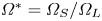 ${\varOmega ^*}=\varOmega _S/\varOmega _L$ is the ratio of their respective rotation rates. We refer the reader to (A1)–(A3) in Appendix A for the full expression of
 $U$ written explicitly in terms of
 ${r^*}$,
 ${h^*}$ and
 ${\varOmega ^*}$. Note that the swimming speed in an Oldroyd-B fluid (i.e. the expression found in Binagia & Shaqfeh Reference Binagia and Shaqfeh2021) can be recovered by setting
 $\varPsi _2=0$ (i.e.
 $B=0$) and noting that
 ${De_{SO}}={De}\,(1-\beta )$.
We can rewrite (1.2) such that the first and second normal stress coefficients of the fluid,  $\varPsi _1$ and
 $\varPsi _2$, appear as dependent variables:
 \begin{equation} \varPsi_1\left(1+\frac{2\varPsi_2}{\varPsi_1}\right) = \frac{2 U' \mu_0}{\varOmega_S^2 R_L\, f({r^*},{h^*},{\varOmega^*})}, \end{equation}
where  $U'$ is the dimensional swimming speed. From this equation, one can clearly see how the elastic properties of the fluid (
 $\varPsi _1$ and
 $\varPsi _2$) can be determined from a measurement of the robot's speed
 $U'$ for a prescribed tail rotation rate
 $\varOmega _S$. We note that for most polymeric fluids of interest,
 $|\varPsi _2|/\varPsi _1 \ll 1$ (a common heuristic is
 $\varPsi _2=-0.1 \varPsi _1$) (Bird et al. Reference Bird, Armstrong and Hassager1987; Morrison et al. Reference Morrison2001), so the left-hand side of (1.3) simplifies to just
 $\varPsi _1$. Thus, assuming
 $\varPsi _2 \approx 0$, one can measure directly
 $\varPsi _1$ so long as the viscosity
 $\mu _0$ is known.
Alternatively, one can also determine both  $\varPsi _1$ and
 $\varPsi _2$ simultaneously by measuring both the swimmer's speed
 $U'$ and the rotation rate of the head (which itself will depend on the rheology of the fluid) for a single experiment. This fact can be appreciated by deriving an asymptotic expression for the head rotation rate directly in terms of
 $\varPsi _1$ and
 $\varPsi _2$ (in a process identical to that done for the swimming speed but now balancing torques rather than forces acting on the swimmer):
 \begin{equation} \bar{\varOmega}_L={r^*}^3\,\dfrac{1-\dfrac{1}{(1+{r^*}+{h^*})^3} -\dfrac{2(\varPsi_1 \varOmega_S/(2\mu_0))^2}{15}\,(1-2\varPsi_2/\varPsi_1)^2}{1-\dfrac{{r^*}^3}{(1+{r^*}+{h^*})^3}}, \end{equation}
where we have defined a dimensionless head rotation rate  $\bar {\varOmega }_L=\varOmega _L/\varOmega _S={\varOmega ^*}^{-1}$. Note that if we take the limit
 ${h^*}\rightarrow \infty$ and
 ${De_{SO}}=0$, then we can confirm
 $\bar {\varOmega }_L={r^*}^3$ (which is the expected result in the case of a Newtonian fluid with zero hydrodynamic interactions).
Thus, just as was the case for (1.3) and the swimming speed, we now have a direct relationship between the head rotation rate and rheological parameters of the fluid. This means that if, for example, the viscosity of a fluid is known, then (1.3) and (1.4) can be solved simultaneously as a system of two equations for the variables  $\varPsi _1$ and
 $\varPsi _2$ after measuring the swimming speed and head rotation of our swimmer for a prescribed tail rotation rate. We point out that the potential to measure both
 $\varPsi _1$ and
 $\varPsi _2$ is especially exciting in the field of rheology where traditionally measurements of
 $\varPsi _2$ have proved quite challenging, requiring both fine instrument sensitivity (since typically
 $|\varPsi _2|\ll \varPsi _1$) as well as unique instrument configurations (Morrison et al. Reference Morrison2001). Furthermore, recently proposed methods for measuring the normal stress coefficients – e.g. measuring the speed of a rotating dumbbell (Pak et al. Reference Pak, Zhu, Brandt and Lauga2012) or the relative force between two microrheological probes (Khair & Squires Reference Khair and Squires2010) – require that two independent measurements be made to compute both
 $\varPsi _1$ and
 $\varPsi _2$; in contrast, both
 $\varPsi _1$ and
 $\varPsi _2$ can be computed from a single experiment in our methodology since we can observe simultaneously two measurable quantities (speed and head rotation rate) that each depend on the rheological parameters of the fluid in a distinctive independent manner (i.e. comparing (1.3) and (1.4)).
Finally, while the theoretical expressions above were derived in the context of a single-mode fluid, the extension to a multi-mode model is straightforward. The effect of the multiple modes can be shown to be additive, such that their impact on the swimming speed is captured completely by the mean of their individual effects. Put more precisely, the swimming speed for the swimmer immersed in a multi-mode fluid is given by (1.3) but with the Deborah number  $De$ now defined in terms of the average relaxation time of the fluid,
 ${De}=\bar {\lambda }\varOmega _S$. This allows us to make direct comparisons between experimental data, where the fluid is fit to a multi-mode constitutive equation, and theory using a single-mode fluid.
1.2. Description of experiments
A small robot was constructed that is capable of untethered self-propulsion in viscoelastic fluids (figures 1a,c) at low  $Re$ (
 $Re = 0.1\unicode{x2013}1$). The robot was designed in two modules: the head (spherical, 70 mm diameter) and a number of tails (most emphasis here is on the 30 mm diameter spherical tail). The counter-rotation between the head and tail was achieved via a stepper motor and microcontroller placed in the head. The propulsion of the swimmer was tested in several fluids. For each fluid, the robot was tuned for neutral buoyancy (see Appendix D) and centre of mass location (see Appendix E), such that it can swim predominantly horizontally as shown in figure 2(a) (e.g. propulsive thrust and gravity are approximately perpendicular to one another). In particular, we confirmed that zero self-propulsion was observed in a viscous Newtonian fluid, i.e. corn syrup (cf. figure 2). To test the swimmer in a viscoelastic fluid, approximately 3 gallons of a polyacrylamide-based ‘Boger’ fluid (Boger & Walters Reference Boger and Walters2012) was was prepared so as to minimize the degree of shear-thinning present in the fluid and thus to isolate the effects of fluid elasticity on propulsion. The composition of our Boger fluid was 92.5 % corn syrup (Karo syrup), 7.4 % deionized water, and 0.1 % polyacrylamide (molecular weight
 $5\times 10^6\,{\rm g}\,{\rm mol}^{-1}$) by weight. The rheology of the fluid was measured using an ARES-G2 rheometer (the raw data of which may be found in Appendix G). A fit to the stress relaxation after a step-strain yielded a longest relaxation time
 $\lambda _{long}\approx 2.51$ s. A multi-mode fit to the small-amplitude oscillatory shear data using three modes (
 $n=3$) yields solvent viscosity
 $\mu _s=2.05$ Pa s, zero-shear solution viscosity
 $\mu _0=4.46$ Pa s, viscosity ratio
 $\beta =0.46$, and average relaxation time
 $\bar {\lambda }=({\sum }_{i=0}^n \lambda ^{(i)} \mu _p^{(i)})/({\sum }_{i=0}^n \mu _p^{(i)})=1.38$ s. A Giesekus mobility parameter for each mode,
 $\alpha _m^{(i)}$, was determined through a fit to the shear rheology data (specifically
 $\varPsi _1$), yielding
 $\alpha _m^{(0)}=0.2$,
 $\alpha _m^{(1)}=0.0002$ and
 $\alpha _m^{(2)}=0.1996$. Note that for the single-mode Giesekus equation,
 $B=-2\varPsi _2/\varPsi _1=\alpha _m$ (Bird et al. Reference Bird, Armstrong and Hassager1987), showing that a fluid with a non-zero value of
 $\alpha _m$ exhibits not only shear-thinning but also a non-zero second normal stress difference. Finally, a power-law fluid model was fit to the shear viscosity data to ascertain the degree of shear-thinning present in the fluid. A shear-thinning exponent 0.93 was found, indicating a very modest degree of shear-thinning present in the fluid. Based on this and the fact that the largest shear rate experienced in the robot experiments is in fact
 ${\dot \gamma }_{max}=2\varOmega _S\approx 2\,{\rm rad}\,{\rm s}^{-1}$ (i.e. the shear rate present at the equator of the small sphere), we conclude that this fluid meets our criteria for an elastic fluid with minimal shear-thinning.
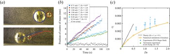
(a) Image analysis (circle detection) was used to determine the trajectory of the swimmer (and thus its propulsion speed) as a function of time. (b) For different tail rotation speeds, the coordinates of the centre of mass were tracked as a function of time. (c) Dimensionless swimming speed  $U$ as a function of the Deborah number
 $De$. The asymptotic theory, valid for small
 $De$, is shown as the dashed black line and assumes an infinite domain and zero shear-thinning in the fluid. Experimental data are shown as the blue dots, with error bars denoting the standard deviation of measurements over repeated trials. Simulations (orange circles) are performed with a multi-mode Giesekus model (which allows for shear-thinning and second normal stress differences in the fluid), with the mesh domain defined to match approximately the size of the experimental tank (the confinement ratio is
 $C=2R_L/W=0.32$).

2. Results
2.1. Characterization of propulsion speed
As described in the preceding section, the swimming speed of the robot is related directly to the elasticity of the fluid.Thus it is critical to assess how the speed of the robotic swimmer compares to that predicted by theory and simulations, since the latter two may then be used to infer properties of the fluid based on observed swimming speeds. In figure 2(c), the dimensionless swimming speed  $U$ of the robot is plotted as a function of the Deborah number (
 $De$) of the fluid,
 $De =\bar {\lambda } \varOmega _S$. Experimental data, shown as the blue dots in figure 2(c), are plotted alongside our small
 $De$ asymptotic theory (black dashed line) and our numerical simulations (orange circles). To compare experiments, both the theory and simulations take as input the specific geometry of the robotic swimmer and the rheology of the fluid:
 ${h^*}=0.17$,
 ${r^*}=0.43$,
 $\bar {\lambda }=1.38$ s and
 $\beta =0.46$.
Some minimal scatter in experimental data (figure 2b) arises from our imaging system (e.g. the camera attempting to refocus due to the presence of bubbles, etc.) and image analysis (lighting, shadows). Transient effects from the swimmer starting and stopping are cropped prior to analysis, and we focus only on regions of steady operation. Raw data in figure 2(b) demonstrate that the propulsive effects are very linear for  $De\approx 0.5\unicode{x2013}1.5$, while the robot is operating at a constant rotation rate, indicating that the transient effects from elastic instabilities are minimal in this
 $De$ range.
From figure 2(c), we observe that both experiments and simulations predict a modest increase in dimensionless swimming speed as a function of the Deborah number  $De$. The asymptotic theory agrees with numerical simulations for small
 $De$, but the two depart as
 $De$ increases. Note that the
 $De$ at which the two depart from one another is smaller than that in Binagia & Shaqfeh (Reference Binagia and Shaqfeh2021) since the present simulations account for shear-thinning present in the fluid and swimmer confinement effects, both of which are neglected in the present theory. We remark that the asymptotic theory for the swimming speed could also be improved by considering higher-order terms in the series expansion, e.g. terms of
 $O({De}^2)$, through computation of the surrounding flow field through
 $O({De}^2)$. The good agreement between simulations and experiments serves as a validation for the computational model and thus allow us to make claims about the propulsion mechanism through an analysis of the numerical results.
2.2. Propulsion mechanism
The propulsion mechanism of this device is related directly to the first normal stress coefficient (e.g. see (1.2)). However, it is not immediately clear how normal stresses in the fluid are generating swimmer thrust mechanistically.
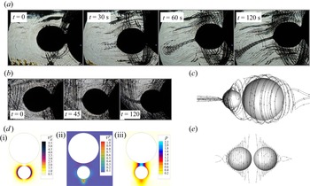
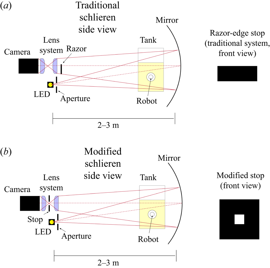
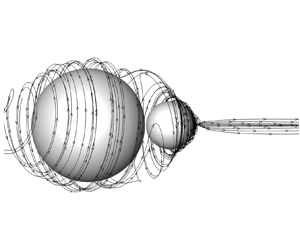
To investigate further, we imaged the robot using a slightly modified schlieren imaging set-up. As shown in figures 3(a,b), features of the flow indicate that a narrow viscoelastic jet develops behind the tail of the robot over a period of tens of seconds. Significant flow in the azimuthal direction (i.e. around the spinning tail) is also visible as dark strands around the small sphere; such flow is predicted to generate regions of large hoop stress around the tail of the swimmer (Binagia & Shaqfeh Reference Binagia and Shaqfeh2021).
(a) Schlieren imaging was used to image features of the flow field in experiments. Shortly after the rotation of the small sphere is initiated ( $t=0$,
 $t=30$), we observe the formation of hoop-like strands around the small sphere and the creation of a slender jet-like structure at the pole of the small spherical tail. As time progresses (
 $t=60$), the jet is seen to persist and grow in length. Even at long times (
 $t=120$), this jet structure is still present behind the rear of the swimmer. (b) We have repeated this imaging process with multiple trials and observe the formation of this jet each time. (c) Numerical simulations visualizing the streamlines of the flow also indicate the presence of an elastic jet. Parameter values used are
 $\beta =0.46$,
 ${De}=2$,
 ${r^*}=0.43$ and
 ${h^*}=0.17$. (d) Polymer stress and pressure in the surrounding flow field: (i) trace of the polymer stress tensor
 $\tau _{ii}^p$; (ii)
 $zz$ component of the polymer stress
 $\tau ^p_{zz}$; (iii) pressure
 $p$. To facilitate visualization, the simulations used the single-mode Giesekus equation with
 $\alpha _m=0.035$ (the value of
 $\alpha _m$ yielding the best single-mode fit to the shear rheology data). (e) When the head and tail are identical in size, the jet structures appear at both head and tail.

Numerical simulations indicate a set of fluid structures that match those seen in the experiments (figure 3c). Simulations suggest that while hoop stresses seem to dominate the polymer stress (figure 3d-i), a non-negligible polymer stress develops along the swimming direction ( $\tau _{zz}^p$, figure 3d-ii) in the region of the viscoelastic jet, precisely where a large pressure wake shown to drive propulsion is located (Binagia & Shaqfeh (Reference Binagia and Shaqfeh2021) and figure 3d-iii).
While the elastic properties of the fluid enable the robot to propel itself, it is the interaction between the solid bodies (specifically, in the context of an asymmetry between the head and the tail) and the nonlinearity of this viscoelastic fluid that enable it to form a primary jet and region of high pressure behind the tail. Figure 3(e) demonstrates this concept, showing that when the head and tail are of equal size, there exist two such jets also of equal size, and each expels fluid from the head and tail, with no net propulsion. Fundamentally, the formation of each jet is a manifestation of the Weissenberg effect (Bird et al. Reference Bird, Armstrong and Hassager1987; Boger & Walters Reference Boger and Walters2012).
2.3. Geometric optimization
In the interest of maximizing the propulsion of our robotic swimmer, we conducted numerical simulations for a range of tail shapes and geometries. Since the speed is the primary signal used in inferring the rheological parameters of the fluid when using the robot as a fluid sensor, maximizing the speed for a given relative rotation rate and fluid rheology is equivalent to maximizing the signal-to-noise ratio of the robot as a measurement device.
Three distinct tail shapes were considered in this process: spherical tails, cylindrical tails and conical tails (specifically, cones with the tip of the cone removed, otherwise known as a conical frustum). Sequential least squares programming (Kraft et al. Reference Kraft1988) was used to determine which tail geometries to simulate, with the algorithm proceeding until a local maximum was reached in the swim speed. Note that the optimal shape of the sphere (i.e.  ${r^*}=0.75$) has been determined in prior work (Binagia & Shaqfeh Reference Binagia and Shaqfeh2021). To reduce the computational cost of the optimization procedure, the single-mode rather than multi-mode Giesekus equation was used, with the same value of
 $\beta =0.46$ but now with
 $\alpha _m=0.035$ (determined from fitting the single-mode model to the shear rheology data). These locally optimal shapes were then used to determine the swimmer's speed as a function of
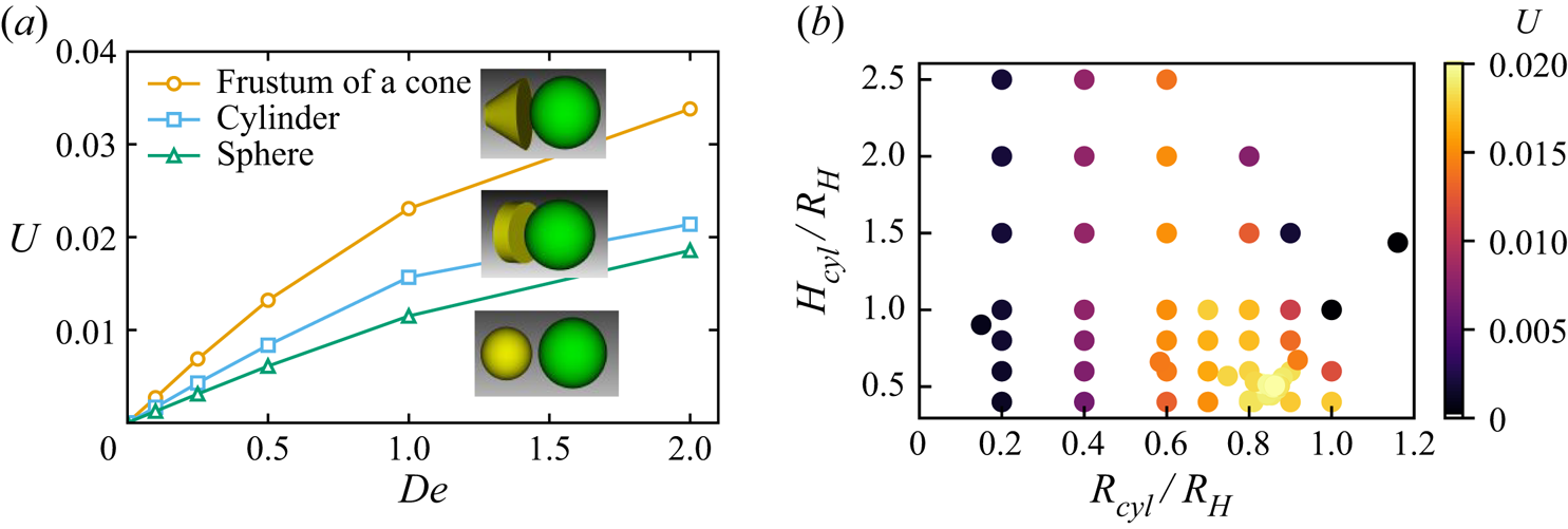
 $De$, as shown in figure 4. We see that for all
 $De$, the speed of the optimal cylindrical tail is strictly greater than the optimal spherical tail; likewise, the speed of the conical frustum is always greater than that of the cylindrical tail. This figure suggests that the swimming speed of the robot with an optimal spherical tail could be more than doubled by constructing a tail in the shape of a frustum.
(a) Dimensionless swimming speed  $U$ as a function of
 $De$ for various tail shapes. For all
 $De$, the swimmer with optimal cylindrical tail (
 $R_{cyl}/R_H=0.86$ and
 $H_{cyl}/R_H=0.51$, where
 $R_H$ denotes the radius of the spherical head) is faster than that with the optimal spherical tail (
 ${r^*}=0.75$). Likewise, the swimmer with the optimal conical frustum tail (
 $R_{1,fr}/R_H=1.0$,
 $R_{2,fr}/R_H=0.31$,
 $H_{fr}/R_H=1.1$, where
 $R_{1,fr}$ is the radius closest to the head) is faster than that having the cylindrical tail for all
 $De$. The insets depict the optimal geometry for each shape family. (b) The set of cylindrical tail shapes that were considered in finding the locally optimal tail used in (a). The optimization procedure was performed at
 $De = 1$ and
 ${h^*}=0.17$.

It is noted that the conical tail shape itself contains a fore–aft asymmetry (therefore may be generating its own net propulsive flow), whereas the cylindrical and spherical tail shapes are generating their propulsion only via flow interactions with the head. At these low  $Re$ (
 $\ll 1$) and weak
 $De$ (
 $O(0.1)\unicode{x2013}O(1)$), the spherical or cylindrical tails are not generating any net propulsive force in isolation. This may not be the case at very high
 $De$ or
 $Re$; for example, Rogowski et al. (Reference Rogowski, Ali, Zhang, Wilking, Fu and Kim2021) demonstrate that a sphere rotating at very high
 $De$ is capable of spontaneous symmetry-breaking. Such effects do not play an important role in this low
 $De$ regime, but they do suggest that the optimal tail geometry will likely change based on the
 $De$ range. We expect that this would especially be the case in very high
 $De$ and
 $Re$ regimes, where new nonlinearities arise from polymer stress instabilities.
3. Discussion
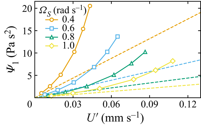
Mimicking attributes of microbiological swimmers, we have built an untethered swimmer that adapts passively to propel itself at different speeds, depending on the properties of the surrounding fluid. In this way, the behaviour itself acts passively as a sensor to the observer. The functionality of this system implies a clear application: a swimming rheometer. Figure 5 depicts a design curve, constructed from our simulation data and our theoretical results at low Deborah number. Observation of the propulsive speed of the robot ( $x$-axis) is a direct measure of the first normal stress coefficient. This is exemplified by (1.3), where the rheology parameter that we want to infer (i.e.
 $\varPsi _1+2\varPsi _2$) is written directly as a function of observables (the swimmer's speed and tail rotation rate) and known quantities (i.e. the swimmer's geometry, the viscosity of the fluid, etc.). Furthermore, very often it is the case in polymeric fluids that
 $|\varPsi _2| \ll \varPsi _1$ (Bird et al. Reference Bird, Armstrong and Hassager1987), so upon assuming
 $\varPsi _2 \approx 0$, (1.3) yields a direct expression for
 $\varPsi _1$ based upon swim speed observations of our swimming robot.
The value of the first normal stress coefficient  $\varPsi _1$ that the robot infers as it is observed to swim at (dimensional) speed
 $U'$ at a tail rotation rate
 $\varOmega _S$. Here, we consider the viscosity to be known a priori from independent measurements (
 $\mu _0=4.46$ Pa s). The dashed lines denote predictions from our low-
 $De$ theory (i.e. (1.3) with
 ${h^*}=0.17$,
 ${r^*}=0.43$, and assuming
 $\varPsi _2\approx 0$). The solid lines and markers are predictions from our numerical simulations using the multi-mode Giesekus equation (i.e. the simulation data shown in figure 2, using the fact that
 $\varPsi _1=2\sum \lambda ^{(i)} \mu ^{(i)}_p$ for a multi-mode model). This figure illustrates the operating characteristics of the swimming robot in terms of its use as a sensor. For example, operating at a small value of
 $\varOmega _S$ (e.g.
 $\varOmega _S=0.4$) allows the robot to be more sensitive to small changes in
 $U'$ but necessarily requires a greater experimental resolution of the observed swimming speed.

To provide a proof of concept for our swimming rheometer, we can compare the inferred values of  $\varPsi _1$ based on the swimmer observations to that which we obtain from a bench-top rheometer. Using (1.3), we obtain predictions of
 $\varPsi _1$ (again assuming here
 $\varPsi _2\approx 0$) equal to 4.3, 3.1, 2.7 and 2.5 Pa
 $\mathrm {s}^2$ for the four different tail speeds. It should be emphasized at this point that typical commercial rheometers cannot measure
 $\varPsi _1$ at these low shear rates (Morrison et al. Reference Morrison2001). For this reason, we compare these measured values of
 $\varPsi _1$ from our swimming rheometer to that predicted by a multi-mode Giesekus fit at shear rates corresponding to the average shear rate created by a sphere rotating at rotation rate
 $\varOmega _S$. This fit to the bench-top rheometer data predicts the ‘true’ values of
 $\varPsi _1$ to be 3.1, 2.2, 1.8 and 1.7 Pa
 $\mathrm {s}^2$. This comparison between our inferred values of
 $\varPsi _1$ from experiments and those predicted from a fit to
 $\varPsi _1$ measurements taken using a commercial rheometer are in reasonable agreement, considering the assumptions of our asymptotic theory used to derive (1.3), and considering that
 $\varPsi _1$ is a dimensional quantity that can range across many orders of magnitude (Bird et al. Reference Bird, Armstrong and Hassager1987; Morrison et al. Reference Morrison2001). The eventual miniaturization of such devices could open numerous opportunities for applications in microbiology, environmental sensing and medical diagnostics.
Supplementary movies
Supplementary movies are available at https://doi.org/10.1017/jfm.2022.485.
Funding
M.P. thanks the Gordon and Betty Moore Foundation (grant no. 5762) and the NSF/UCSF award for the Center for Cellular Construction project (grant no. 9917sc). E.S.G.S. acknowledges that this work is also supported in part by the National Science Foundation (NSF) grant no. CBET 1803765. J.P.B. acknowledgements support from the Stanford Office of the Vice Provost for Graduation Education and the Gerald J. Lieberman fellowship.
Declaration of interests
The authors report no conflict of interest.
Author contributions
L.A. Kroo and J.P. Binagia contributed equally to this work.
Appendix A. Derivation of the swimming speed at small  $De$

For sufficiently small  $De$, the swimming speed can be predicted via an asymptotic theory developed by Binagia & Shaqfeh (Reference Binagia and Shaqfeh2021). While we refer the interested reader to Binagia & Shaqfeh (Reference Binagia and Shaqfeh2021) for the details of the derivation, we will summarize briefly the main ideas and results for this analytical theory since it is used frequently in the present work. The main result is a prediction for the dimensionless velocity of the swimmer
 $U_z$:
 \begin{equation} U_z = U_z^0+U_z^{(HO)}, \end{equation}
where
 \begin{equation} U_z^{0} = {De}\,(1-\beta)\,\dfrac{(1+{h^*})^2{r^*}^3(1+{h^*}+3{r^*}){\varOmega^*}^2-{r^*}({h^*}+{r^*})^2(3+{h^*}+{r^*})}{(1+{r^*})(1+{h^*}+{r^*})^5{\varOmega^*}^2} \end{equation}
and
 \begin{equation} U_z^{(HO)} = {De}\,(1-\beta){r^*}^3\left(\dfrac{Q}{3(1+{r^*})(1+{h^*}+{r^*})^7{\varOmega^*}^2}\right). \end{equation}
The factor  $Q$ in the numerator of (A3) is given by
 $$\begin{gather} Q({r^*},{h^*},\varOmega^*)={-}3+15{h^*}+6{h^*}^2+2{h^*}^3+15{r^*}+12{h^*}{r^*}+6{h^*}^2{r^*}+6{r^*}^2+6{h^*}{r^*}^2\nonumber\\ +\,2{r^*}^3-\left[2(1+{h^*})^3+6(1+{h^*})^2{r^*}+15(1+{h^*}){r^*}^2-3{r^*}^3\right]{\varOmega^*}^2. \end{gather}$$
We use the subscript  $z$ to denote the fact that the velocity is in the vertical
 $z$-direction, i.e. along the axis of rotation (cf. figure 1b). These equations are written in terms of several key dimensionless numbers, including the ratio of the sizes of the two spheres
 ${r^*}=R_S/R_L$, the dimensionless separation between the two spheres
 ${h^*}=h_{sep}/R_L$, and the ratio of the spheres’ rotation rates
 ${\varOmega ^*}=\varOmega _S/\varOmega _L$. As discussed in Binagia & Shaqfeh (Reference Binagia and Shaqfeh2021), this expression for the swimming speed is derived by considering far-field hydrodynamic interactions between two spheres rotating in isolation at
 $Re=0$. The flow field for a sphere is assumed to be the leading-order viscoelastic flow for a rotating sphere in Stokes flow (Bird et al. Reference Bird, Armstrong and Hassager1987). Furthermore, since we are considering a weakly elastic flow, we assume that the hydrodynamic drag for each sphere is simply that given by Stokes’ drag law (Kim & Karrila Reference Kim and Karrila2013). To enforce the fact that the swimmer should be torque-free, we set
 $\varOmega ^*=(1/{r^*})^3$, a relationship that is derived by equating the dimensional torque that each sphere experiences when rotating at
 $Re=0$ in a Newtonian fluid, i.e.
 $8{\rm \pi} \mu _0 \varOmega R^3$. Despite these simplifying assumptions, it is shown in Binagia & Shaqfeh (Reference Binagia and Shaqfeh2021) that this simple analytical theory agrees with numerical simulations up to
 ${De} \approx 1$ for a wide range of values for the viscosity ratio
 $\beta$; this is likely a consequence of the fact that the disturbance flow created by the rotation of each sphere decays relatively rapidly for problems of this kind, decaying as
 $1/r^2$, where
 $r$ is the distance from the centre of each sphere. Finally, we remark that for all of the sets of parameters considered in Binagia & Shaqfeh (Reference Binagia and Shaqfeh2021) as well as in the present work,
 $U_z>0$, corresponding to propulsion in the direction of the large sphere.
The equations above were derived in the context of the Oldroyd-B constitutive equation and are thus written in terms of the rheological parameters  $\mu _p$ and
 $\lambda$; however, it is quite straightforward to express these results in terms of another common constitutive equation, the second-order fluid (SOF) model. The SOF model, which applies to slowly varying flows, is derived formally by applying the retarded motion expansion to a given flow and retaining terms quadratic in the velocity gradient (Bird et al. Reference Bird, Armstrong and Hassager1987). The deviatoric stress (i.e.
 $\boldsymbol {\tau }=\beta (\boldsymbol {\nabla }\boldsymbol {u} + \boldsymbol {\nabla }\boldsymbol {u}^{\rm T}) + \boldsymbol {\tau }^p$) for the SOF model is given by
 \begin{equation} \boldsymbol{\tau}=\boldsymbol{\dot{\gamma}}-{De_{SO}}\left({\stackrel{\triangledown}{\boldsymbol{\dot{\gamma}}}}+B \boldsymbol{\dot{\gamma}}\boldsymbol{\cdot} \boldsymbol{\dot{\gamma}}\right), \end{equation}
where  $\boldsymbol {\dot {\gamma }}=\boldsymbol {\nabla }\boldsymbol {u} + \boldsymbol {\nabla }\boldsymbol {u}^{\rm T}$,
 ${De_{SO}}=(\varPsi _1 \varOmega _S)/(2\mu _0)$ is the Deborah number defined for the SOF model,
 $B=-2\varPsi _2/\varPsi _1$, and
 $\varPsi _1$ and
 $\varPsi _2$ are the first and second normal stress coefficients, respectively. Note that because
 $\lambda ={\varPsi _1}/{2\mu _p}$ ,
 ${De_{SO}}={De}\,(1-\beta )$ (Bird et al. Reference Bird, Armstrong and Hassager1987). From (A5), it is clear that the second-order fluid model captures the first deviations from Newtonian behaviour (where simply
 $\boldsymbol {\tau }=\boldsymbol {\dot {\gamma }}$).
Binagia & Shaqfeh (Reference Binagia and Shaqfeh2021) showed that the swimming speed for the two-sphere swimmer is proportional to the radial disturbance flows created by each rotating sphere. The leading-order radial flow created by a rotating sphere in a viscoelastic fluid is identical for the Oldroyd-B and second-order fluid models; written dimensionlessly in terms of the parameters of the latter, it is  $u_r={De_{SO}}\,(1-B)[(1/2r^2-3/2r^4+1/r^5)(3\cos ^2\theta -1)]$ (Bird et al. Reference Bird, Armstrong and Hassager1987). We can write this in terms of the Oldroyd-B fluid by noting that
 $\varPsi _2=0$ (and hence
 $B=0$) for the Oldroyd-B fluid, and
 ${De_{SO}}={De}(1-\beta )$, so
 $u_r={De}(1-\beta )[(1/2r^2-3/2r^4+1/r^5)(3\cos ^2\theta -1)$. Binagia & Shaqfeh (Reference Binagia and Shaqfeh2021) presented this final result, which is linear in
 ${De}(1-\beta )$ (since the swimming speed is proportional to the radial flow velocity in this asymptotic theory), but we will now allow for non-zero
 $\varPsi _2$, such that in general the swimming speed takes the form
 \begin{equation} U = |U_z| = {De_{SO}}\,(1-B)\,f({r^*},{h^*},{\varOmega^*}), \end{equation}
where  $f({r^*},{h^*},{\varOmega ^*})$ captures the complex dependence on the geometry and kinematics of the swimmer (i.e. as shown in (A1)–(A3)). Writing the expression for speed in this way, in terms of
 $\varPsi _1$ and
 $\varPsi _2$, allows us to rearrange explicitly for these direct measures of the rheology of the fluid:
 $$\begin{gather} \frac{U'}{\varOmega_S R_L} = \left(\frac{\varPsi_1 \varOmega_S}{2 \mu_0}\right)(1+2\varPsi_2/\varPsi_1)\,f({r^*},{h^*},{\varOmega^*}), \end{gather}$$
 $$\begin{gather}\varPsi_1+2\varPsi_2 =\frac{2 U' \mu_0}{\varOmega_S^2 R_L\,f({r^*},{h^*},{\varOmega^*})}. \end{gather}$$
Equation (A8) illustrates how rheological properties of the fluid ( $\varPsi _1$ and
 $\varPsi _2$) can be inferred directly from a measurement of the dimensional swimming speed
 $U'$ of the robot for a given tail rotation rate
 $\varOmega _S$. It also illustrates how the geometry of the swimmer, i.e. the function
 $f({r^*},{h^*},{\varOmega ^*})$, affects directly the mapping between the measured speed
 $U'$ and the inferred properties
 $\varPsi _1$ and
 $\varPsi _2$; in other words, the geometry should be selected carefully to maximize the utility of the device as a sensor for the fluid. We note at this point that unless one assumes
 $\varPsi _2\approx 0$,
 $\varPsi _1$ and
 $\varPsi _2$ cannot both be determined via (A8); rather, we can compute only the sum
 $\varPsi _1+2\varPsi _2$. As we will discuss in the next appendix, however, an independent measurement of the head rotation rate of the swimmer provides an additional equation that, when solved alongside (A8), allows one to determine uniquely both the values of
 $\varPsi _1$ and
 $\varPsi _2$.
Finally, while expressions (A7) and (A8) were derived in the context of a single-mode fluid, the extension to a multi-mode model is straightforward. The effect of the multiple modes can be shown to be additive, such that their impact on the swimming speed is captured completely by the mean of their individual effects. Put more precisely, the swimming speed for the swimmer immersed in a multi-mode fluid is given by (A1)–(A3), but with the Deborah number  $De$ now defined in terms of the average relaxation time of the fluid,
 ${De}=\bar {\lambda }\varOmega _S$. This allows us to make direct comparisons of experimental data, where the fluid is fit to a multi-mode constitutive equation, with simulations and theory for a single-mode fluid.
Appendix B. Derivation of the head rotation rate at small $De$

An expression for the rotation rate of the head (i.e. the larger sphere) can be obtained by enforcing the torque-free condition on the swimmer. In the case of two spheres rotating in a Newtonian fluid at  $Re=0$ and neglecting hydrodynamic interactions, the balance is simply
 \begin{equation} {-}8{\rm \pi} \mu_0 R_L^3 \varOmega_L+8{\rm \pi} \mu_0 R_S^3 \varOmega_S=0, \end{equation}
where again  $\varOmega _L$ and
 $\varOmega _S$ denote the magnitudes of the rotation rates. Thus in a Newtonian fluid at Stokes flow, the ratio of the rotation rates is
 $\varOmega _L/\varOmega _S=(R_S/R_L)^3={r^*}^3$. Of course, there will be a modification to the torque experienced by each sphere when rotating in a viscoelastic fluid; Walters & Waters (Reference Walters and Waters1963, Reference Walters and Waters1964a,Reference Walters and Watersb) have performed a perturbation expansion for a sphere rotating in a third-order fluid and found that the hydrodynamic torque
 $L'$ experienced by the sphere is given by
 $$\begin{align} L'&={-}8{\rm \pi} \mu_0 R^3 \varOmega\left[ 1 + \frac{Re^2}{1200}+\frac{Re\,{De_{SO}}}{140}\left(1+\frac{b_{11}}{b_2}\right)-\frac{2\,De_{SO}^2}{15}\left(1+\frac{b_{11}}{b_2}\right)^2\right.\nonumber\\ &\quad\left.-\,\frac{24\,De_{SO}^2}{5}\,\frac{b_1(b_{12}-b_{1:11})}{b_2^2}\right], \end{align}$$
where  $b_1$,
 $b_{12}$,
 $b_{1:11}$ and
 $b_{2}$ are parameters of the third-order fluid model (Bird et al. Reference Bird, Armstrong and Hassager1987). Here,
 $Re={\rho R^2 \varOmega }/{\mu _0}$ and
 ${De_{SO}}=(\varPsi _1\varOmega )/(2\mu _0)=-b_2\varOmega /b_1$. For
 $Re=0$, we can rewrite this as
 \begin{equation} L'={-}8{\rm \pi} \mu_0 R^3 \varOmega\left[ 1-\frac{2\,De_{SO}^2}{15}\,(1+B)^2-\frac{24\,De_{SO}^2}{5}\,(B_{12}-B_{1:11})\right], \end{equation}
where  $B=b_{11}/b_2=-2\varPsi _2/\varPsi _1$,
 $B_{12}=b_{12}b_1/b_2^2$ and
 $B_{1:11}=b_{1:11}b_1/b_2^2$. From this equation, it is readily apparent that as the elasticity of the fluid increases (increasing
 $De$), the hydrodynamic torque experienced by the rotating sphere decreases. In summary, each sphere experiences a Newtonian torque
 $L_{newt}'=8{\rm \pi} \mu _0 R^3 \varOmega$ and an additional torque from rotating in an elastic fluid,
 $L_{elastic}'$:
 \begin{equation} L_{elastic}'=8{\rm \pi} \mu_0 R^3 \varOmega\left[ \frac{2\,De_{SO}^2}{15}\,(1+B)^2+\frac{24\,De_{SO}^2}{5}\,(B_{12}-B_{1:11})\right]. \end{equation}
The final contribution that we would like to consider in our torque balance is that from hydrodynamic interactions. Note that for this, we need consider only hydrodynamic interactions given by the Newtonian disturbance flow created by each sphere; this is because to leading order, fluid elasticity has zero effect on the azimuthal component of velocity for a rotating sphere (Bird et al. Reference Bird, Armstrong and Hassager1987). Indeed, given the alignment of our spheres in the vertical direction, the only component of velocity that can alter the torque experienced by the other sphere is the azimuthal component. Applying Faxén's law for the hydrodynamic torque applied to one sphere as a result of the disturbance flow from the other sphere (Kim & Karrila Reference Kim and Karrila2013), we obtain the following contributions to the torque on each half of the swimmer's body:
 $$\begin{gather} L_{HI,L}'={-}8{\rm \pi} \mu_0 R_L^3 \left( \frac{R_S^3 \varOmega_S}{(R_S+R_L+h_{sep})^3}\right), \end{gather}$$
 $$\begin{gather}L_{HI,S}'=8{\rm \pi} \mu_0 R_S^3 \left( \frac{R_L^3 \varOmega_L}{(R_S+R_L+h_{sep})^3}\right). \end{gather}$$
Note that interactions between the two spheres reduce the net hydrodynamic torque that either of them experiences. A negative sign appears in the expression for  $L_{HI,L}'$ given the convention that we have taken in figure 1(b), where the larger sphere is seen to have a positive angular velocity with respect to the vertical
 $z$-axis (and thus the torque applied by the smaller sphere will act in the negative
 $z$-direction, in alignment with its negative angular velocity).
We can combine each of the above contributions into a total torque balance on the swimmer:
 $$\begin{gather} L_L' + L_S' = 0, \end{gather}$$
 $$\begin{gather}L_{newt,L}'+L_{elastic,L}'+L_{HI,L}'+L_{newt,S}'+L_{elastic,S}'+L_{HI,S}'=0, \end{gather}$$
 $$\begin{gather} -8{\rm \pi} \mu_0 R_L^3 \varOmega_L \left[1+ \frac{R_S^3 (\varOmega_S/\varOmega_L)}{(R_S+R_L+h_{sep})^3}-\frac{2\,De_{SO}^2}{15}\left(\frac{\varOmega_L}{\varOmega_S}\right)^2(1+B)^2\right.\nonumber\\ \hspace{-8pc}\left.-\frac{24\,De_{SO}^2}{5}\left(\frac{\varOmega_L}{\varOmega_S}\right)^2(B_{12}-B_{1:11})\right]\nonumber\\ \hspace{12pt}+\,8{\rm \pi} \mu_0 R_S^3 \varOmega_S\left[ 1+\frac{R_L^3 (\varOmega_L/\varOmega_S)}{(R_S+R_L+h_{sep})^3} -\,\frac{2\,De_{SO}^2}{15}\,(1+B)^2\right.\nonumber\\ \hspace{-7.3pc}\left.-\,\frac{24\,De_{SO}^2}{5}\,(B_{12}-B_{1:11})\right]=0. \end{gather}$$
In dimensionless form:
 $$\begin{align} &-\bar{\varOmega}_L\left[1+ \frac{{r^*}^3 \bar{\varOmega}_L^{{-}1}}{(1+{r^*}+{h^*})^3}-\frac{2\,De_{SO}^2}{15}\,\bar{\varOmega}_L^2(1+B)^2-\frac{24\,De_{SO}^2}{5}\bar{\varOmega}_L^2\,(B_{12}-B_{1:11})\right]\nonumber\\ &\quad +{r^*}^3\left[ 1+\frac{\bar{\varOmega}_L}{(1+{r^*}+{h^*})^3} -\frac{2\,De_{SO}^2}{15}\,(1+B)^2-\frac{24\,De_{SO}^2}{5}\,(B_{12}-B_{1:11})\right]=0, \end{align}$$
where we have defined a dimensionless head rotation rate  $\bar {\varOmega }_L=\varOmega _L/\varOmega _S$. Here,
 ${De_{SO}}=(\varPsi _1\varOmega _S)/(2\mu _0)$ is defined using the rotation rate of the small sphere (the ‘tail’ of the swimmer) as is done in the rest of the paper. At this point, we can simplify the torque balance by noting the following. We know from the torque balance in a Newtonian fluid that
 $\bar {\varOmega }_L \sim {r^*}^3$. Thus the elastic contribution to the torque on the small sphere is of size
 $O(De_{SO}^2)$, while that on the large sphere is
 $O({r^*}^9 De_{SO}^2)$. Since
 ${r^*} \le 1$, clearly the latter will be significantly smaller than the former and can be neglected safely. That leaves us with the expressions
 $$\begin{gather} -\bar{\varOmega}_L\left[1+ \frac{{r^*}^3 \bar{\varOmega}_L^{{-}1}}{(1+{r^*}+{h^*})^3}\right] +{r^*}^3\left[1+\frac{\bar{\varOmega}_L}{(1+{r^*}+{h^*})^3} -\frac{2\,De_{SO}^2}{15}\,(1+B)^2\right.\nonumber\\ \hspace{-8pc}\left.{}-\frac{24\,De_{SO}^2}{5}\,(B_{12}-B_{1:11})\right]=0, \end{gather}$$
 $$\begin{gather} {r^*}^3\left[ 1 -\frac{2\,De_{SO}^2}{15}\,(1+B)^2-\frac{24\,De_{SO}^2}{5}\,(B_{12}-B_{1:11})-\frac{1}{(1+{r^*}+{h^*})^3}\right]\nonumber\\ \hspace{-8pc}=\bar{\varOmega}_L\left(1-\frac{{r^*}^3}{(1+{r^*}+{h^*})^3}\right). \end{gather}$$
Solving for  $\bar {\varOmega }_L$:
 \begin{equation} \bar{\varOmega}_L={r^*}^3\,\dfrac{\left( 1-\dfrac{1}{(1+{r^*}+{h^*})^3} -\dfrac{2\,De_{SO}^2}{15}\,(1+B)^2-\dfrac{24\,De_{SO}^2}{5}\,(B_{12}-B_{1:11})\right)} {1-\dfrac{{r^*}^3}{(1+{r^*}+{h^*})^3}}. \end{equation}
This result shows that, in contrast to the swimming speed, fluid elasticity has no effect on the rotation rate of the large sphere to leading order (i.e. at  $O(De)$). Rather, the effect of elasticity manifests at
 $O({De}^2)$ and leads to a reduction in the dimensionless rotation rate of the large sphere. Note that if we take the limit
 ${h^*}\rightarrow \infty$ and
 ${De_{SO}}=0$, then we can confirm that we obtain
 $\bar {\varOmega }_L={r^*}^3$ (which is what we expect in the case of a Newtonian fluid and zero hydrodynamic interactions). This equation can also be simplified if we wish to omit the third-order fluid parameters by setting
 $B_{12}=0$ and
 $B_{1:11}=0$ (i.e. in effect considering only the second-order fluid model):
 \begin{equation} \bar{\varOmega}_L={r^*}^3\,\dfrac{\left( 1-\dfrac{1}{(1+{r^*}+{h^*})^3} -\dfrac{2\,De_{SO}^2}{15}\,(1+B)^2\right)}{1-\dfrac{{r^*}^3}{(1+{r^*}+{h^*})^3}}. \end{equation}
This form of the equation is useful when we consider the application of our swimmer as a rheometer for the fluid since now the only rheological parameters appearing on the right-hand side are  $\varPsi _1$ and
 $\varPsi _2$ via the definitions of
 ${De_{SO}}$ and
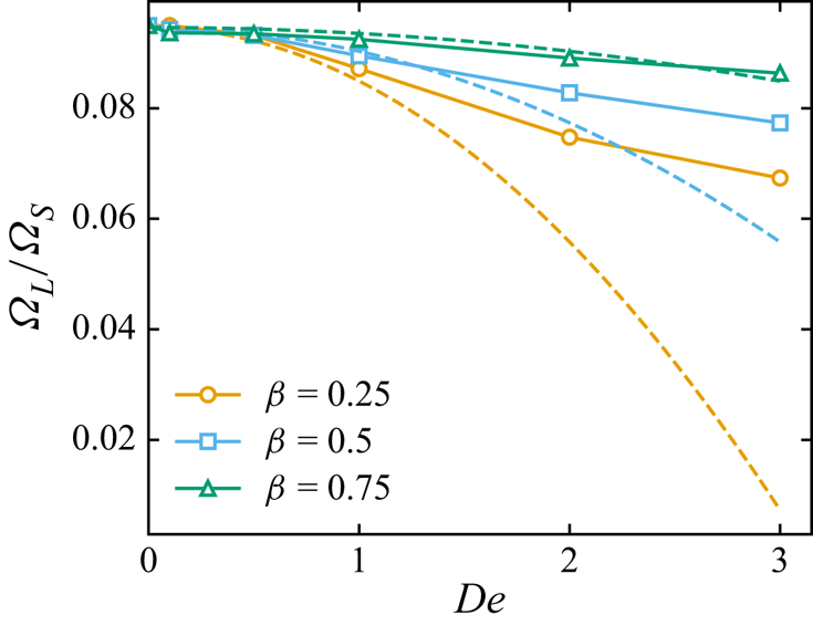
 $B$, respectively. We can confirm the formula presented in (B14) by comparing it to numerical simulations using the single-mode Oldroyd-B equation, as shown in figure 6. To compare figure 6 to numerical simulations using the Oldroyd-B equation, we note that for the Oldroyd-B equation
 $\varPsi _2=0$, thus
 $B=0$, and furthermore that the Deborah number defined for the Oldroyd-B equation, i.e.
 ${De}=\lambda \varOmega _S$, is related to that for the second- and third-order fluid models via
 ${De_{SO}}=(1-\beta )\,{De}$. The agreement between the theory and simulations suggests that our asymptotic equation is indeed an accurate measure of the head rotation rate for small
 $De$.
Rotation rate of the head of the swimmer ( $\varOmega _L$) normalized by that of the tail (
 $\varOmega _S$) as a function of the Deborah number (
 $De$) and the viscosity ratio (
 $\beta$). The markers denote numerical simulations, while the dashed lines denote the asymptotic theory, i.e. (B14); both consider
 ${h^*}=0.05$ and
 ${r^*}=0.5$.

Appendix C. Robot design
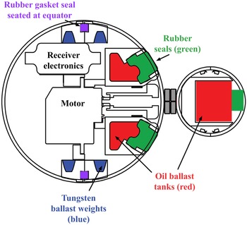
The 70 mm ‘head’ contains all power and electronics for the system, including a pseudo-closed-loop speed control system consisting of a small stepper motor and gearbox. The initial versions of the robot were constructed within molded polypropylene spherical shells to ensure high geometric precision of the exterior, to match with simulations and theory. Both the head and tail modules required ballast tanks for tuning the buoyancy and centre of mass of the robot. As shown in figure 7, these tanks were accessible from the exterior, and use rubber seals, which allow the user to inject or withdraw fluid repeatedly from the ballasts at multiple points on the robot.
Methods for buoyancy tuning. Oil ballast tanks (red) are used for fine tuning during experiments, by the user injecting small volumes of oil into the tanks (displacing air) through a rubber stopper. Modular tungsten weights are used in the head for large adjustments, but these large adjustments require a moderate amount of disassembly.

The head and tail are coupled with a magnetic linker shaft (thus the design includes no rotary shaft seal). This allows the robot to be highly configurable and modular, specifically allowing for quickly swapping tail attachments without any modification to the robot. Because the system has closed-loop speed control (and is not power-limited), effects of friction in the magnetic linker do not significantly affect the system performance.
The device is powered with small lithium polymer batteries, with an onboard voltage regulator, microcontroller, IR receiver and stepper motor driver. Speed control protocols can be uploaded to the onboard microcontroller, and transmitted during experiments with a modified IR remote control (transmitter modified from 940 nm to 850 nm to avoid significant absorption from the submersion fluid). The robot is capable of receiving signals at significant distances while fully submerged (tested to approximately 0.5 m without receiver difficulty).
Appendix D. Maintaining neutral buoyancy
One important design aspect of this device is a practical way to tune its mass easily/precisely. Because the forward motion of the swimmer is a crucial measurement signal, it is necessary to either know the sum of the forces acting on the robot due to gravity and buoyancy a priori, or, if this information is not known, tune these forces to be as close to zero as possible prior to use.
In our prototype device, we tune the mass of the robot to achieve neutral buoyancy in two stages: gross and fine. In the first stage of gross tuning, the head of the robot is taken apart into two hemispheres. The sphere comes apart in these two discrete halves, with a (compressible) rubber gasket at the equator. In each half, there are slots along the interior for tungsten ballast weights, and tungsten putty. This allows tuning of mass in the range approximately 20–60 g from the initial base weight. This gross mass change allows the device to be tuned for a variety of submersion fluids that vary widely in density.
In the second stage of buoyancy tuning, fine adjustments can be made (of the order of 0.1 g). This is achieved by adding oil to small tanks on the device. After gross adjustments (when the device is fully assembled and often submerged in the fluid), a sharp needle is used to penetrate a rubber ‘vacutainer’ seal, and oil can be added in the tail or to two locations in the head. The seal self-heals when the needle is removed, and can be used for thousands of use cycles. As the oil tanks themselves are non-compliant, very small and watertight, a release needle (to allow for air to escape) is also necessary when adding fluid to the oil ballasts. This two-stage method allows for very fine control over the buoyancy of the laboratory prototype, which is necessary to achieve good measurement signal.
The same two-step buoyancy tuning method is also used on the tail attachments. It is proposed that active buoyancy control would be ideal in this circumstance, although difficult to achieve on such small-scale prototypes (automatically self-adjusting the mass of the swimmer while in use, based on the density of the submersion fluid). For very-small-scale device versions, it seems feasible to manufacture a series of devices with unique densities – and subsequently choose the most appropriate device based on the submersion fluid.
Appendix E. Centre of mass tuning: trim and stability
In addition to tuning the overall mass of the swimmer, it is necessary to consider the exact position of the centre of mass in the robot.
Another way of phrasing this: it is ideal if the distance (along the swimming axis) between the centre of gravity and the centre of buoyancy is minimized. The centre of gravity will be located at the centre of mass of the robot (including the mass of the magnetic linker, which is not negligible). The centre of buoyancy will be located at the geometric/volumetric centre of the robot in a homogeneous submersion fluid, and more generally, at the centre of mass of the fluid that the device is displacing.
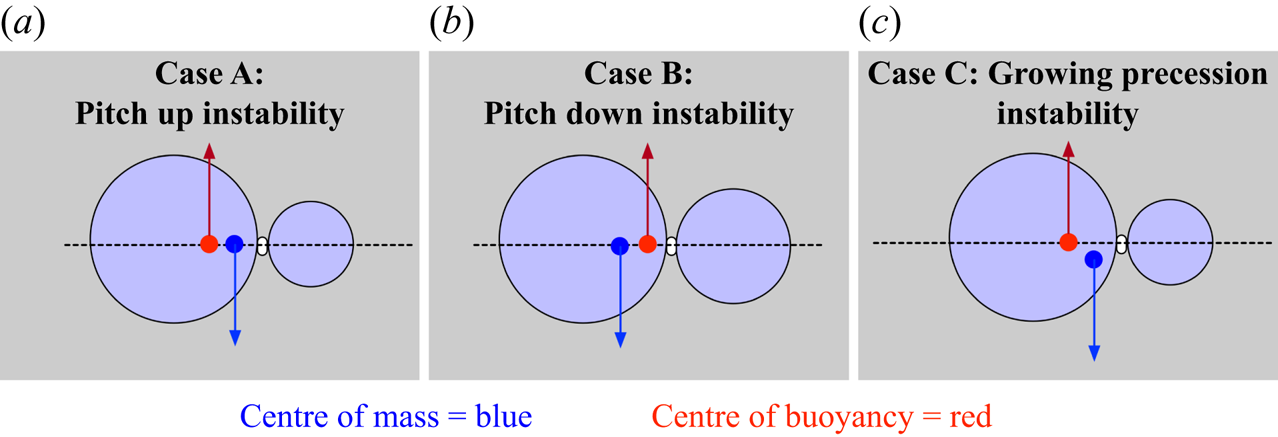
Even if the total mass of the robot is nearly perfectly tuned, the tail will have a tendency to pitch up or down relative to the forward motion vector of the device (especially once the device begins to propel forward), if the relative mass between the head and tail has not also been considered. The presence of these instabilities (detailed further in figure 8) decreases/obfuscates the apparent forward propulsion, lowering the accuracy of the device if not taken into account carefully.
Modes of swimmer instability.

Investigations into the stability of the swimmer are ongoing. We have observed experimentally that tails of larger diameters (0.5 times the head sphere and larger) are far more sensitive to this effect than smaller diameter tails.
The balancing rig, pictured in figure 9, was used just prior to experimental data collection to ensure that the centre of mass within the head was precisely centred to avoid the unstable case in figure 8(c).
Balancing rig for aligning the head's centre of mass along the swimming axis.

This sensitivity to centre of mass (on- and off-axis) is challenging to overcome in horizontal swimming modes. We have now begun to move towards vertical swimming modalities where the swimmer swims downwards in the fluid, such that the centre of mass and centre of buoyancy are easier to tune on-axis (these data are not pictured).
Appendix F. Schlieren imaging of fluid flow
A slightly modified schlieren imaging system was constructed to visualize features in the flow, as shown in the main text.
The use of multiple edges at the stop (instead of a single razor blade) allows us to see gradients along both  $x$- and
 $y$-axes.
The refracted angle of a beam interacting with a finite element at  $(x,y)$ can then be written as the sum
 \begin{equation} \theta = \dfrac{1}{n} \int \left( \left| \dfrac{\partial n_{x,y}}{\partial y} \right| +\left| \dfrac{\partial n_{x,y}}{\partial x} \right| \right)\,{\rm d}z, \end{equation}
where  $n_{x,y}$ is the index of refraction in a specific finite element of the tank. The contrast in figure 10 is a threshold function of the refracted angle,
 $\theta$. Edges on both sides of the aperture allow both positive and negative gradients along that axis to achieve the same effect in refraction angle (absolute values on terms).
Imaging system for capturing fluid features in the Boger fluid.

Changes in the index of refraction in this system may be caused by several factors. We expect that minor heterogeneity in the fluid flow (which will tend to propagate along the flow direction) will highlight the flow structures visually. This is a well-known property of water-based Boger fluids; however, it has a minimal rheological effect (for example, samples from different parts of the tank will have indistinguishably similar storage and loss moduli). Another possibility is that the polymer stress is inducing mesoscale lensing in the fluid, leading to regions that tend to appear darker where large changes in polymer stress are present (hoop stress region, viscoelastic jet). The latter possibility is under further study within our group, and warrants further careful investigation.
Appendix G. Formulation and rheology of the non-Newtonian Boger fluid
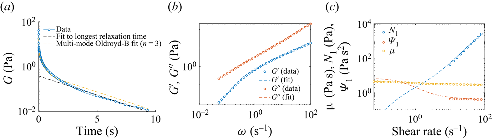
A model viscoelastic fluid, i.e. a ‘Boger’ fluid (Boger & Walters Reference Boger and Walters2012), was prepared to minimize shear-thinning in the rheological properties and thus to isolate the effects of fluid elasticity on propulsion. The composition of our Boger fluid was 92.5 % corn syrup (Karo syrup), 7.4 % deionized water, and 0.1 % polyacrylamide (molecular weight  $5\times 10^6\,{\rm g}\,{\rm mol}^{-1}$) by weight. The rheology of the fluid was measured using an ARES-G2 rheometer and is shown in figure 11. Several experiments were conducted to characterize the fluid on an ARES-G2 rheometer, including stress relaxation after a step strain (figure 11a), small-amplitude oscillatory shear (figure 11b), and steady shear (figure 11c). Stress relaxation after a step strain (figure 11a) was used to determine the longest relaxation time of the fluid. This longest relaxation time was found to be
 $\lambda _{long}\approx 2.51$ s. With the relaxation time determined, a multi-mode Oldroyd-B model was fit to the small-amplitude oscillatory shear data shown in figure 11(b), with the total zero-shear solution viscosity determined by the value of the shear viscosity
 $\mu$ at the lowest measured shear rate (cf. figure 11c). A summary of the fit is provided in table 1. This fit yields solvent viscosity
 $\mu _s=2.05$ Pa s, zero-shear solution viscosity
 $\mu _0=4.46$ Pa s, viscosity ratio
 $\beta =0.46$, and average relaxation time
 $\bar {\lambda }=1.38$ s. In situations where we wish to model shear-thinning in the fluid and a non-zero second normal stress coefficient
 $\varPsi _2$, we fit the shear rheology shown in figure 11(c) to either a single-mode or a multi-mode Giesekus model. The fit to the single-mode Giesekus equation (which was fitted to the shear viscosity) yields a best fit value
 $\alpha _m=0.035$, and the fit to the multi-mode Giesekus equation with
 $n=3$ (which was fitted to the data for
 $\varPsi _1$) yields
 $\alpha _m^{(0)}=0.2$,
 $\alpha _m^{(1)}=0.0002$ and
 $\alpha _m^{(2)}=0.1996$. This fit is shown as the yellow dashed line in figure 11(c). Note that for the single-mode Giesekus equation,
 $B=-2\varPsi _2/\varPsi _1=\alpha _m$ (Bird et al. Reference Bird, Armstrong and Hassager1987), showing that a fluid with a non-zero value of
 $\alpha _m$ exhibits not only shear-thinning but also non-zero second normal stress difference. Finally, a power-law fluid model was fit to the shear viscosity data presented in figure 11(c) to ascertain the degree of shear-thinning present in the fluid. A shear-thinning exponent 0.93 was found, indicating a very modest degree of shear-thinning present in the fluid. Based on this and the fact that the largest shear rate experienced in the robot experiments is in fact
 ${\dot \gamma }_{max}=2\varOmega _S\approx 2\,{\rm rad}\,{\rm s}^{-1}$ (i.e. the shear rate present at the equator of the small sphere), we concluded that this fluid meets our criteria for an elastic fluid with minimal shear-thinning.
Rheological characterization of the viscoelastic Boger fluid used in this study. (a) Stress relaxation after a step strain of 500 %. Benchtop rheometer data of the relaxation modulus, G, is shown as a function of time. Shown alongside the data (blue markers) are a fit to the longest relaxation time of the fluid (black dashed line) and the prediction from the multi-mode Oldroyd-B fit with  $n=3$ (yellow dashed line). (b) Small-amplitude oscillatory shear experiment to characterize the linear viscoelastic response of the fluid (i.e. the storage and loss moduli
 $G'$ and
 $G''$). Raw data are shown as markers, with the multi-mode fit shown as dashed lines. (c) Nonlinear shear rheology of the fluid, i.e. the shear viscosity
 $\mu$, the first normal stress difference
 $N_1$, and the first normal stress coefficient
 $\varPsi _1$. The largest shear rate in the experiments was
 ${\dot \gamma }_{max}=2\varOmega _S\approx 2\,{\rm rad}\,{\rm s}^{-1}$ (i.e. the shear rate present at the equator of the small sphere). The dashed lines denote predictions from the multi-mode Giesekus equation with
 $\alpha _m^{(0)}=0.2$,
 $\alpha _m^{(1)}=0.0002$ and
 $\alpha _m^{(2)}=0.1996$ for the nonlinear rheology (the
 $\alpha _m^{(i)}$ being determined from a fit to the data for
 $\varPsi _1$).

Summary of the multi-mode fit to the rheological data presented in figure 11. Note that these values of  $\lambda ^{(i)}$ and
 $\mu ^{(i)}_p$ are relevant for both a multi-mode Oldroyd-B and Giesekus fit since the two predict the same linear viscoelastic response (i.e.
 $G'$ and
 $G''$). The multi-mode Giesekus fit consists of these parameters plus the following values for the mobility parameters for each mode (determined from a fit to the nonlinear rheology, figure 11c):
 $\alpha _m^{(0)}=0.2$,
 $\alpha _m^{(1)}=0.0002$ and
 $\alpha _m^{(2)}=0.1996$.

Appendix H. Numerical simulations
For the numerical calculations, the methodology follows largely that described in Binagia & Shaqfeh (Reference Binagia and Shaqfeh2021) and is summarized briefly below. Three-dimensional simulations of the governing equations and boundary conditions are conducted through the use of a third-order-accurate finite volume flow solver developed at Stanford's Center for Turbulence Research (Ham et al. Reference Ham, Mattsson and Iaccarino2006). This code has been tested thoroughly for accuracy and robustness for a wide range of problems, including viscoelastic flows (Richter, Iaccarino & Shaqfeh Reference Richter, Iaccarino and Shaqfeh2010; Padhy et al. Reference Padhy, Shaqfeh, Iaccarino, Morris and Tonmukayakul2013; Yang et al. Reference Yang, Krishnan and Shaqfeh2016), deformable particles (Saadat et al. Reference Saadat, Guido, Iaccarino and Shaqfeh2018), and active swimmers (Binagia et al. Reference Binagia, Guido and Shaqfeh2019, Reference Binagia, Phoa, Housiadas and Shaqfeh2020; Housiadas et al. Reference Housiadas, Binagia and Shaqfeh2021). The problem is solved in the co-moving frame of reference, wherein the swimmer is stationary in a uniform flow, such that we may use a body-fitted mesh for our computational domain. The evolution equation for the conformation tensor is solved using the log-conformation method (Fattal & Kupferman Reference Fattal and Kupferman2004; Hulsen, Fattal & Kupferman Reference Hulsen, Fattal and Kupferman2005), and for boundary conditions for the conformation tensor, we set  $\boldsymbol {c}=\boldsymbol {I}$ at the entrance to the domain and utilize a convective outlet boundary condition at the exit. To resolve the stress boundary layers present near the swimmer, we use an unstructured tetrahedral mesh with increasing resolution towards the centre of the domain (where the swimmer is located). We have performed mesh convergence studies to ensure that results are independent of the choice of mesh size. The swimming speed
 $U$ and rotation rate of the large sphere
 $\varOmega _L$ are determined by advancing the equations of motion forward in time, solving for
 $U_z$ and
 $\varOmega _L$ at each time step such that
 $F_z=0$ and
 $L_z=0$ via a quasi-Newton iteration – specifically, Broyden's method (Broyden Reference Broyden1965).
Appendix I. Secondary effects on the swimming speed: confinement and shear-thinning
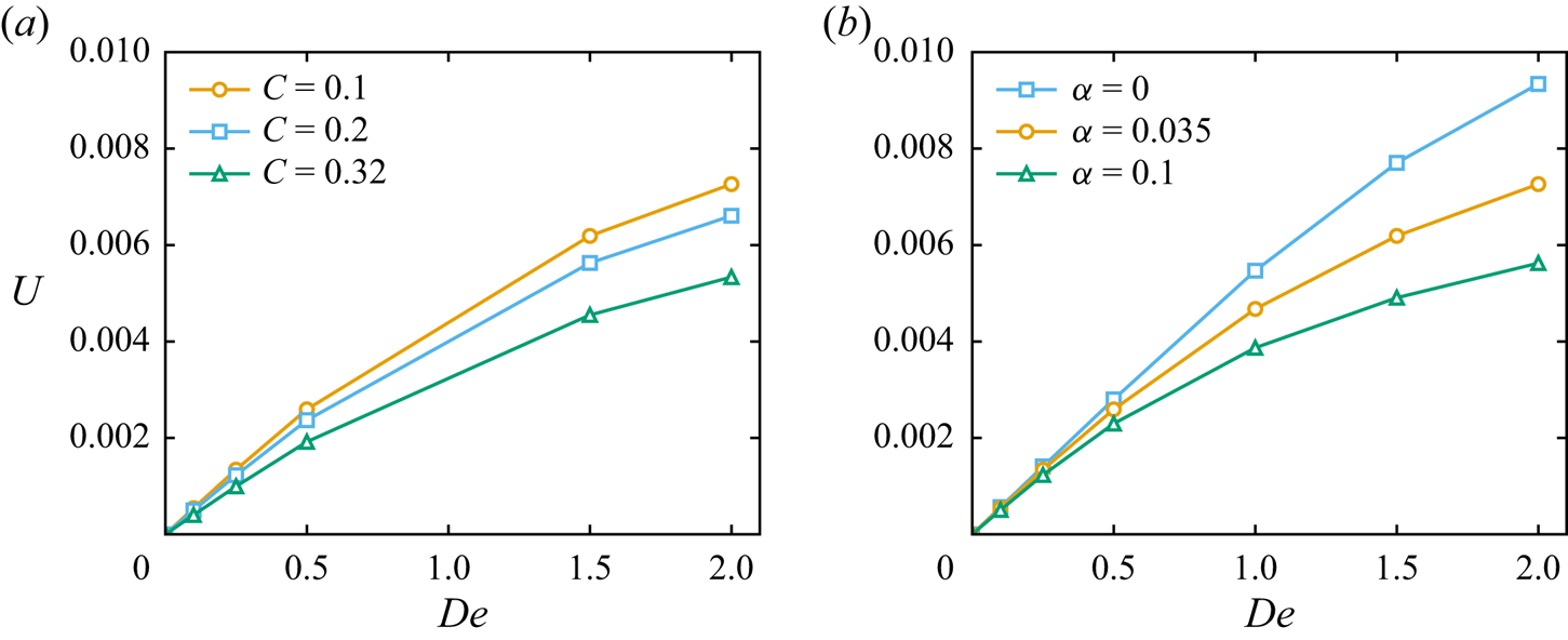
As discussed in the main text, two effects not considered in the numerical simulations of our previous work (Binagia & Shaqfeh Reference Binagia and Shaqfeh2021) but now included in the present work are shear-thinning rheology and confinement of the swimmer. From figure 12(a), we see that as the confinement around the swimmer  $C=2R_L/W$ increases, the swimming speed decreases for all
 $De$. From figure 12(b), we see that as
 $\alpha _m$ increases (corresponding to a larger extent of shear-thinning and larger value of
 $\varPsi _2$ for the fluid), the swimming speed decreases for all
 $De$. Note that for
 $\alpha _m=0$, corresponding to the Oldroyd-B constitutive equation, the fluid exhibits zero shear-thinning and
 $\varPsi _2=0$. In summary, both increasing confinement and increasing the extent of shear-thinning present in the fluid are seen to decrease the swimmer's speed in a viscoelastic fluid.
(a) Effect of confinement  $C=2R_L/W$ on the swimming speed
 $U$. Simulations were performed using the single-mode Giesekus constitutive equation with
 $\alpha _m=0.035$,
 $\beta =0.46$,
 ${r^*}=0.43$ and
 ${h^*}=0.17$. As the confinement around the swimmer increases (i.e. increasing
 $C$), the swimming speed is observed to decrease. (b) Effect of the Giesekus mobility parameter
 $\alpha _m$ on the swimming speed
 $U$. For non-zero values of
 $\alpha _m$, the Giesekus equation exhibits shear-thinning and a non-zero second normal stress coefficient. Simulations for (b) were performed using the single-mode Giesekus constitutive equation with
 $C=0.1$,
 $\beta =0.46$,
 ${r^*}=0.43$ and
 ${h^*}=0.17$. We find that as
 $\alpha _m$ increases, the speed of the swimmer decreases for all
 $De$.

Appendix J. Simulations with a conical frustum tail
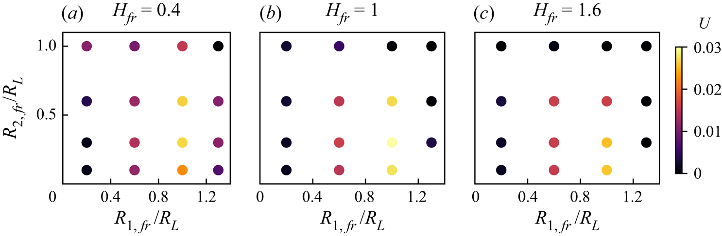
In figure 13, we visualize the simulations conducted for various conical frustum tail shapes. From these plots, we see that a relatively large frustum radius near the head is desirable (the optimal value of  $R_{1,fr}/R_L$ is 1.0), while a smaller radius seems to be desirable near the rear of the swimmer (the optimal value of
 $R_{2,fr}/R_L$ being 0.31). In contrast to the dependence on the radii, the dependence on the length of the cone is much less substantial, with the optimal cone length
 $H_{fr}/R_L=1.1$.
For the optimization study of the frustum, a three-dimensional shape space must be explored. Here we show, for three different cone height values, the forward speed as a function of the other two geometric parameters ( $R_{1,fr}$ and
 $R_{2,fr}$), and the radii of the circular cross-sections at each end of the tail (where
 $R_{1,fr}$ refers to the radius closest to the swimmer's head).

Appendix K. Tail shape optimization procedure
To complete optimization of propulsion for tail shapes of various geometries, a mesh and time step convergence study was used to determine the coarsest spatial and temporal dimension that could give a translation speed  $U$ within 15 % of the finest grid result. To run the geometric optimization, many function evaluations are needed, so running many simulations at the finest mesh resolution is infeasible. To generate an initial guess for the optimizer, univariate optimizations were run for all the geometric degrees of freedom (i.e. radius and height of a cylinder). A sequential least-squares programming (SLSP) method was then used with the initial guess to find the global maximum, with a convergence tolerance of
 $1\times 10^{-4}$ with respect to
 $U$. The SLSP method estimates the Jacobian of the objective function at a given point to converge quickly to the function's minimum. To confirm the coarse grid results, multiple points were chosen near the found maximum and were run on both the coarse and fine mesh. These data confirmed that the found maximum on the coarse grid was also a maximum on the fine grid within the chosen convergence tolerance. After the optimization, a sweep of different geometric values was chosen to evaluate the global characteristics of the objective function
 $U$ and to confirm that the global maximum was found.
Appendix L. Using a design curve to measure $\varPsi _1$

Further comments and minor details are included in this appendix, related to the discussion section in the main text about how this device may be used (in a very practical sense) as an untethered rheometric device.
From figure 5, we observe that while the low- $De$ asymptotic theory predicts linear design curves, the numerical simulations appear to be nonlinear with respect to the observed speed; this fact can be appreciated by noting that the curve of
 $\varPsi _1$ versus
 $U'$ is in many ways an inversion of figure 2 (i.e. now speed is on the
 $x$-axis and a measure of the fluid elasticity is on the
 $y$-axis). While the asymptotic theory is advantageous in that it provides a closed-form relationship between
 $\varPsi _1$ and the swimmer's geometry, observed speed, etc., its usage should be confined to cases where the assumptions of its derivation hold (i.e.
 $Re = 0$,
 $De \ll 1$, an unconfined swimmer). In contrast, the curves mapped out by the numerical simulations are valid for finite
 $De$ and can consider arbitrary levels of confinement; however, they define only an implicit relationship between
 $U'$ and
 $\varPsi _1$. In order to use effectively the numerical simulations to create a mapping between
 $U'$ and
 $\varPsi _1$, curve fitting would be required to interpolate between the points at which simulations were conducted.
One consequence of figure 5 is that different robot tail speeds (different values of  $\varOmega _{S}$) should reproduce the same rheological property of the fluid, but with different sensitivities. This is related to the operating conditions: a rotation rate should be chosen such that both the sensitivity of the signal and the desired sensing range are taken into account. This design space may be constructed for other, more efficient tail shapes such as the cylinder.
A corollary associated with this operating curve also holds: if maintaining a constant motor speed and the forward propulsion speed changes in time, this indicates a non-homogeneous fluid, where rheological properties of the fluid are changing spatially. This allows an observer to map non-uniform rheological properties within a region.
Here, we note some minor details in how we arrived at the inferred values of  $\varPsi _1$ based on our experimental observations and using (A8). The experimental data points displayed in figure 2(c) correspond to average tail rotation rates 0.46, 0.73, 0.89 and
 $1.0\,{\rm rad}\,{\rm s}^{-1}$, and swimming speeds 0.036, 0.070, 0.091 and 0.12 mm s
 $^{-1}$. Plugging these values into (A8), we would obtain respective predictions of
 $\varPsi _1$ (assuming here again
 $\varPsi _2\approx 0$) equal to 4.3, 3.1, 2.7 and 2.5 Pa
 $\mathrm {s}^2$, respectively. It should be emphasized at this point that typical commercial rheometers cannot measure
 $\varPsi _1$ at these low shear rates (Morrison et al. Reference Morrison2001). For this reason, we compare our inferred values of
 $\varPsi _1$ from our swimming rheometer to that predicted by our multi-mode Giesekus fit at shear rates corresponding to the average shear rate created by a sphere rotating at rate
 $\varOmega _S$.
The average shear rate for a sphere of radius  $R$ rotating at rate
 $\varOmega$ at
 $Re=0$ is
 \begin{equation} {\dot\gamma}_{avg} = \left(\int_0^{\rm \pi}\left|\frac{{\rm d}u_\phi}{{\rm d}r}\right|_{r=R}{\rm d}\theta\right)\left/\left(\int_0^{\rm \pi} {\rm d}\theta\right)\right.=4\varOmega/{\rm \pi}. \end{equation}
At these shear rates, the fits to the multi-mode Giesekus equation are 3.1, 2.2, 1.8 and 1.7 Pa  $\mathrm {s}^2$. If we take the values from the bench-top rheometer (as predicted by the Giesekus fit) as the ‘ground truth’, then we obtain differences (as compared to values using our swimming robot) 38 %, 43 %, 47 % and 50 %, respectively. Because
 $\varPsi _1$ is a dimensional quantity that can range across many orders of magnitude (Morrison et al. Reference Morrison2001; Bird et al. Reference Bird, Armstrong and Hassager1987), it is also relevant to report that the estimated absolute error on
 $\varPsi _1$ is computed to be
 $0.8\unicode{x2013}1.2$ Pa s
 $^2$ at these low shear rates (under 1 Hz).
This comparison between our inferred values of  $\varPsi _1$ from experiments and those predicted from a fit to
 $\varPsi _1$ measurements taken using a commercial rheometer are in reasonable agreement, considering the assumptions of our asymptotic theory used to derive (A8). It is notable that effectively, the swimming rheometer is providing a direct estimate for
 $\varPsi _1$ at shear rates where commercial rheometers typically cannot. Finally, we remark that as the tail rotation rate decreases, i.e. decreasing
 $De$, the accuracy of our low-
 $De$ theory and formula for
 $\varPsi _1$ increases; indeed, this is manifested clearly above in that we observe the relative percent errors decreasing with decreasing
 $\varOmega _S$.