ASSESSING THE DEGREE OF TRADE PROTECTION

The degree to which an import-competing sector of the economy is protected from foreign competition is a deceptively complex question. The first step in addressing this question is to examine nominal rates of protection. In the late nineteenth century, import tariffs were the sole form of U.S. trade intervention (subsidies and quotas were not employed until later in the twentieth century). The nominal rates of protection are the rates of import duty as set by Congress and applied at the border by customs officials.

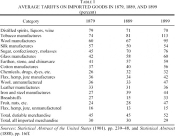
Table 1 shows the average import tariffs with respect to the major import-competing sectors of the economy in 1879, 1889, and 1899. Because the United States was a net exporter of agricultural goods and a net importer of manufactured goods for most of this period, tariffs were imposed mainly on imported manufactured goods and consumption items. The rates of most import duties were very stable over the period from 1870 to 1913. The average tariff on total imports was about 30 percent and the average tariff on dutiable imports was about 45 percent.⁴

The distinction between dutiable and nondutiable imports is important because about one-third of U.S. imports during this time entered the country duty-free, largely because they were goods that did not compete with domestic producers. These included coffee and tea, raw silk and certain hides, India rubber, and tropical fruits such as bananas.

Nominal rates of protection do not necessarily indicate the actual degree of protection given to domestic producers. One problem with nominal rates is that they ignore the structure of protection across industries. The effective rate of protection, defined as the percentage change in value added in an activity as a result of the tariff structure, takes into account the impact of tariffs on intermediate and final goods in determining the degree to which producers of final goods are protected.⁵

Low tariffs on intermediate goods combined with high tariffs on final goods can result in very high effective rates of protection for final goods.

This tendency is evident in the late-nineteenth-century U.S. tariff code. As Table 1 indicates, tariffs on unprocessed raw materials (such as flax and wool) were set lower than duties on final manufactured goods. For example, the duty on unmanufactured wool was about 33 percent, whereas the duty on manufactured wool products was about 67 percent. According to G. R. Hawke's calculations, the effective rate of protection given to domestic wool manufacturers was 229 percent in 1889.⁶

Indeed, his study confirms that, for most U.S. industries during this period, the escalation of the tariff with the level of processing led to much higher effective rates of protection than indicated by the nominal rate of protection. However, a critical shortcoming of the effective rate of protection is that it does not necessarily reflect the magnitude (or even the direction) of the underlying incentive to shift resources into import-competing industries.⁷

A third measure of protection takes the price of nontraded goods as a numeraire against which one can determine the degree of assistance given to import-competing producers and the size of the burden placed upon export-oriented producers. The “net” or “true” rate of protection is defined as the proportionate change in the domestic price of importables relative to nontradeable goods.⁸

Taking I. A. McDougall's and Rudiger Dornbusch's work on tariffs and nontraded goods as a point of departure, Larry Sjaastad and others have shown how a tariff leads to excess demand for nontraded goods, resulting in an increase in their price and an appreciation of the real exchange rate (a decline in the price of traded relative to nontraded goods) as part of the international adjustment mechanism.⁹

To illustrate the concept, consider a small open economy that produces exportables, importables, and nontraded goods. The prices of the traded goods are determined on the world market (the terms of trade), but the prices of the nontraded goods depend on domestic supply and demand. (Thus, there are three relative prices, the terms of trade and the prices of exportables and importables in terms of the nontradeables.) The imposition of an import tariff raises the domestic price of importables relative to exportables and, initially, relative to nontraded goods as well. This higher price shifts resources into the production of importables and out of the production of exportables and nontradeables. It also shifts demand away from importables toward exportables and nontraded goods. The increased demand for and reduced supply of nontraded goods increases the price of nontraded goods in terms of exported goods and mitigates the increase in price of importables relative to nontraded goods.

These price changes are a necessary part of the international adjustment mechanism. An increase in the tariff reduces imports, leading to an incipient balance of trade surplus and excess demand for nontradeables. An appreciation of the real exchange rate (that is, an increase in the relative price of nontraded to traded goods) is required to restore balanced trade and eliminate the excess demand. Because of the higher price of nontradeables, the magnitude of protection given to domestic producers of import-competing goods is less than that indicated by the nominal tariff rate. In addition, producers of exportables face a decline in their price relative to that of nontradeables.

In this framework, the net or true rate of protection is defined as the proportionate change in the domestic price of importables relative to nontradeables. The tariff increases the domestic price of importables by (1 + t), where t is the ad valorem tariff rate, which in turn increases the domestic price of nontradeables by (1 + d), where d is the percentage increase in the price of nontraded goods. As a result, the net protection to the importables sector is

or

Similarly, the net subsidy to the exportables sector is

where s is the rate of export subsidy granted by the government. If s = 0, as in the late nineteenth century, then s* reduces to −d/(1 + d), which will be negative (i.e., an export tax).

For example, suppose that a 50 percent import tariff leads to a 20 percent increase in the price of nontraded goods. This means that the net subsidy to import-competing producers as a result of the tariff (as measured by the increase in the price of importables relative to nontraded goods) is 25 percent, while the net tax imposed on exporters (as measured by the decline in the price of exportables relative to nontradeables) is 17 percent. If the price of nontraded goods had risen by the full amount of the tariff, then the import-competing sector would have received no protection, as its relative price would not have increased.

As is often the case in tax policy, policy makers can choose the nominal rate of protection, but cannot directly control the incidence of the tariff because they cannot influence how much it drives up the price of nontraded goods. In terms of incidence, in the example just considered, only 60 percent of the nominal protection actually reaches import-competing producers as a subsidy, while 40 percent of the nominal protection falls on exporters as an effective export tax. Only if the tariff has no impact on nontraded goods prices will the nominal rate of protection translate into assistance of the same magnitude for import-competing producers.

Furthermore, the following equilibrium relationship can be shown to hold

where P_N is the price of nontraded goods, P_M is the price of importables, P_X is the price of exportables, a ˆ indicates the proportion rate of change (e.g., ΔP_X / P_X). The incidence or shift parameter ω is a function of the compensated demand and supply price elasticities for nontradeables with respect to the three prices.

¹⁰

This incidence or shift parameter ω summarizes the general equilibrium relationship between the prices of traded and nontraded goods and indicates the degree to which importables and nontradeables are substitutes in production and consumption. In general, ω falls between zero and one and indicates the fraction of the increase in the price of importables (with a tariff) that spills over and increases the price of nontradeables. When ω is zero, there is no change in the price of nontradeables as a result of the tariff and hence the price of import-competing goods rises by the amount of nominal protection. As ω approaches one, in which case ΔP_N / P_N will be close to ΔP_M / P_M, implying that import-competing and nontraded goods are close substitutes in production and consumption, there will be little net protection of importables relative to nontradeables.

If import tariffs are the only form of trade intervention, such that there are no export subsidies and therefore ΔP_X / P_X = 0, then from equation 2 we have

Combining equations 1 and 2′ yields

In this equation, the net or true rate of protection hinges on the nominal rate of tariff protection (t) and the incidence parameter (ω). Because 0 ≤ ω ≤ 1, the nominal rate of protection overstates the true degree of protection (t ≥ t* ≥ 0). If ω = 0, then t* = t, but as ω approaches one, then t* approaches zero.

The incidence parameter ω also indicates the proportion of the tariff that is borne by exporters as an implicit export tax. Assuming again that there are no export subsidies, then combining equations 1′ and 2′ yields

If ω = 0, then the price of exportables in terms of nontradeables does not change and exporters do not suffer (i.e., s* = 0), but if ω > 0, then s* < 0. In the limit, if ω = 1, then the price of exportables relative to nontradeables falls by the full extent of the tariff and a nominal tariff of a given amount acts as an export tax of the same amount. Thus, if the tariff has a large impact on the price of nontraded goods, the tariff simultaneously yields a low level of protection for import-competing producers while imposing a great cost on exporters.

Figure 1 illustrates these relationships. The horizontal axis measures the relative price of exportables in terms of nontradeables (P_X / P_N) and the vertical axis measures the relative price of importables in terms of nontradeables (P_M / P_N). In the absence of any trade policy interventions, the domestic price of importables in terms of exportables (P_M / P_X) is given by the world market and is represented by the ray extending from the origin. The schedule HH indicates different combinations of prices of importables and exportables (relative to nontradeables) that clear the market for nontradeable goods. (If the price of importables goes up, then the price of exportables must go down to eliminate the excess demand for nontradeables.) The initial equilibrium is at A where the terms-of-trade ray intersects the HH schedule.

The imposition of an ad valorem import tariff of rate t increases the domestic price of importables relative to exportables, rotating the ray upward by the amount of the nominal tariff. The new equilibrium point is B, where this ray intersects the HH schedule. To remove the incipient tariff-induced trade surplus and accompanying excess demand for nontradeables, the price of nontraded goods increases by d percent. The price of exportables relative to nontradeables falls by 1 / (1 + d) while the price of importables relative to nontradeables increases by (1 + t) / (1 + d).

The magnitude of the increase in price of nontradeables is determined by the degree of substitutability between nontradeables and importables in production and consumption. If there is substitutability between nontraded and traded goods, then HH is negatively sloped.¹¹

Figure 1 also depicts two extreme cases. If importables and nontradeables are perfect substitutes in production and consumption (ω = 1), the HH schedule is horizontal, the price of nontradeables increases by the full extent of the tariff, and the final equilibrium is at C. In this case, the import-competing sector receives no protection, because its relative price did not increase, and the burden of the tariff falls entirely on producers of exportables, whose price falls relative to nontradeables by 1 / (1 + t). This nominal tariff is a pure export tax with no protection for import-competing producers relative to nontradeables.

Alternatively, if exportables and nontradeable are close substitutes (ω = 0), the HH schedule is vertical, the price of nontradeables does not change, and the final equilibrium is at D. In this case, the nominal tariff equals the net or true protection given to import-competing producers. The price of exportables falls relative to importables, but not relative to nontraded goods.

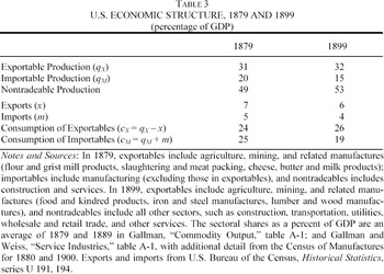
This framework is a useful way of thinking about the late-nineteenth-century American economy for several reasons. First, the U.S. economy at this time can be viewed as being composed of three sectors, producing agricultural goods (exportables), manufactured goods (importables), and nontraded goods (services). These sectors were roughly balanced in terms of size: in 1879, agriculture and mining accounted for 33 percent of GDP, manufacturing about 23 percent of GDP, and services roughly 44 percent of GDP.¹²

Any analysis that goes beyond a simple two-sector tradeoff between the export and import-competing sectors and brings into account another large segment of the economy (the nontraded services sector) is therefore historically relevant.

Second, the impact of protection in raising the price of nontraded goods and inflating the cost structure of the economy is not only commonly recognized today, but was frequently mentioned in the late nineteenth century. The imposition of high trade barriers to protect a large segment of the economy could not help but to have an impact on the nontraded sector of the economy as well. Many observers recognized that increased production in import-competing industries as a result of the tariff would create demands on resources that would increase production costs and thereby mitigate the gains to domestic producers of import-competing goods while adversely affecting exporters. The Special Commissioner for Revenue, David Wells, wrote in his first report that a high import tariff “will soon distribute itself throughout the whole community, and will eventually manifest itself and reappear in the shape of an increased price for all other forms of labor and commodities; thus aggravating the very evil which in the outset it was intended to remedy.”¹³

And William Grosvenor noted: “A duty on one article may not affect at all the cost of producing others. But duties on three thousand articles, each duty being diffused in its effect through a whole community, must have some power to increase the cost of producing every thing, and thus must not only tend to neutralize every benefit contemplated, but to put even our natural industries at a disadvantage.”¹⁴

Third, changes in the real exchange rate were an important part of the international adjustment mechanism in the late nineteenth century. In response to a higher tariff, an alternative adjustment would be a nominal exchange rate appreciation, which would also lower the relative price of tradeables. For most of the late nineteenth century, however, the United States was on the gold standard and so nominal exchange rate changes were ruled out. Instead, changes in the domestic price level, i.e., the price of nontradeables, were required to remove the excess demand for nontraded goods and restore the trade balance to its previous level.¹⁵

MEASURING NET PROTECTION AND TARIFF INCIDENCE

Like the concepts of nominal and effective protection, the net or true rate of protection can be explored with some simple calculations. Because the incidence parameter ω is determined by a complex structure of substitution relationships, a common strategy is to estimate it indirectly by rearranging equation 2 as follows

and estimating

where ω is the elasticity of P_N / P_X with respect to P_M / P_X and ε is an error term. This regression relies on the fact that the terms of trade are determined by the world market whereas the prices of nontraded goods are endogenous.

¹⁶

This equation focuses on how changes in the relative price of imports (as depicted by a rotation of the ray in Figure 1) affect the relative price of nontradeables, but excludes anything that might change the price of domestic nontraded goods without necessarily changing the price of imports or exports. That is, it does not account for factors that might shift the HH schedule itself. A plausible shift variable for domestic prices (the HH schedule) is the domestic money stock, or currency held by the public, relative to nominal GDP. This is a measure of inflationary pressures, as changes in the money supply might bring about changes in domestic prices beyond those induced by changes in the prices of traded goods. Therefore, equation 5 can be modified as follows

where M is the domestic monetary stock relative to nominal GDP.

This method of estimating ω has the advantage of requiring only time series data on export and import prices, the price of nontradeables, and the money supply. Robert Lipsey calculates export and import prices starting in 1879, as presented in U.S. Bureau of the Census, Historical Statistics of the United States, series U-226 and U-238, and Matthew Simon reports a similar series back to 1865.¹⁷

A series representing the price of nontraded goods is not readily available, in part because data on the prices of such goods (which typically include housing and other services) are scarce and have not been collected to create a separate price index. Researchers have typically used a broad price index, such as the GDP deflator or the consumer price index, as largely representative of nontraded goods prices in lieu of data on purely domestic goods prices. In this case, the GDP deflator is taken from the work of Louis Johnston and Samuel Williamson and the consumer price index of Paul David and Peter Solar.¹⁸ The data on the stock of money (currency held by the public) is presented in U.S. Bureau of the Census, Historical Statistics of the United States, series X 410, and nominal GDP is from the Johnston and Williamson series.¹⁹

One concern about this specification is that the results from a regression based on equation (5) or (5′) may be spurious if the relative price series are nonstationary. In results that are not reported, augmented Dickey-Fuller test statistics on the data series confirm that one cannot reject the hypothesis that log(P_M / P_X) and log(P_N / P_X) using either the GDP deflator or CPI have a unit root in levels (i.e., are nonstationary), while one can reject that hypothesis in first difference (i.e., the series are stationary when differenced). Estimation of equation (5) and (5′) in levels might be appropriate if the nonstationary series are cointegrated, i.e., that there is a long-run equilibrium relationship between the two such that a linear combination of them is stationary; otherwise, they should be estimated in first differences to ensure that the regressors are stationary.

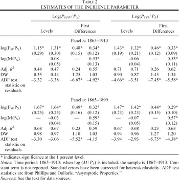
Table 2 presents regression results for equations (5) and (5′) in levels and first differences for the period 1865 to 1913 (in panel a) and 1865 to 1899 (in panel b). The results for the levels regressions suggest that log(P_N / P_X) and log(P_M / P_X) are not cointegrated. Using the approach of Robert Engle and Clive Granger, the augmented Dickey-Fuller test on the residuals of the levels regression indicates that the residuals are nonstationary and hence the levels results are not consistent and may be spurious.²⁰

(The Durbin-Watson test statistic also suggests that the residuals are not stationary.)

In the first-difference regression, both the regressors and the residuals are stationary. In estimating equation 5 for the period 1865 to 1913 (panel a), both measures of nontraded goods prices produce similar point estimates of ω, 0.48 in the case of the GDP deflator and 0.46 in the case of the consumer price index. However, as noted before, these estimates may suffer from omitted variables bias because they do not account for possible changes in domestic prices that occur independently of changes in the prices of traded goods. Hence, results are also reported including log(M / P_X) as in equation (5′), which appears to confirm the bias of the previous estimates. With the inclusion of this variable, the estimate of ω falls to 0.34 in the case of the GDP deflator and 0.33 in the case of the consumer price index, and the explanatory power of the regression improves considerably.

One concern with these estimates is that the structure of U.S. trade underwent a dramatic shift starting in the mid-1890s when the United States became a net exporter of manufactured goods. To ensure that the estimates of ω are not affected by this problem, panel b reports the same regression results for the period 1865 to 1899. Regardless of the general price index used, the estimates of ω are similar to those in panel a: about 0.46 in first regression and about 0.31 in the second regression controlling for inflationary pressures.

Thus, depending upon which specification is preferred, the high estimate of ω is about 0.45 and the low estimate of ω is about 0.32. With an average tariff on total imports of 30 percent, equation (2′) indicates that these duties would push up the price of nontradeables by 14 percent under the high estimate of ω and by 10 percent under the low estimate of ω. Is it plausible that import tariffs were at such a high level as to have raised the prices of nontraded goods by about 10 to 14 percent? Most accounts of this period put the level of U.S. prices as substantially higher than those in free-trade Britain. Marianne Ward and John Devereux report that the prices of services (housing, domestic service, and transportation) were roughly 25 percent higher in the United States than in Britain during the late nineteenth century, despite the similar income levels in the two countries.²¹

In 1910 the nominal dollar-sterling exchange rate was $4.86, but Jeffrey Williamson calculates the purchasing power parity exchange rate was 30 percent higher at $6.35, reflecting trade impediments and higher U.S. nontraded goods prices.²² These would be upper-bound indicators of the possible impact of tariffs on the price of nontradeables. Higher import tariffs may indeed have contributed in part to the higher price level in the United States.

Using equations 3 and 3′ results in estimates of ω that the nominal rate of protection of 30 percent translates into a 15 percent degree of net protection given to import-competing producers (manufacturing) and amounts to a 12 percent effective tax on exporters (agriculture) in the case of the high ω, and a 19 percent degree of net protection and 9 percent export tax in the case of the low ω. As expected, import tariffs were not nearly as protective as indicated by nominal or effective rates of protection and the burden imposed on the exportables sector was significant.

These results have implications that help explain several well-known features of the nineteenth-century debate over tariff policy. The advantages effectively gained by the import-competing producers, as compared to nontraded goods producers, were much lower than might be deduced from the nominal rates of protection. Just as agricultural subsidies in the twentieth century get capitalized into land values and the prices of other inputs, thereby raising farmers' costs, the import tariffs of the late nineteenth century put upward pressure on producers' costs by increasing nominal wages and the prices of nontraded goods. As a result, import-competing interests had an incentive to press for even higher tariffs to gain greater protection.²³

The results also indicate that exporters faced a substantial export tax, on the order of about 10 percent. The term ω indicates the fraction of protection that is borne by exporters; meaning that about 30 to 40 percent of whatever nominal import tariffs were imposed resulted in a higher price of nontraded goods with no compensating change in the price of exportable goods. Although the Constitution formally prohibited export taxes, agriculture faced a large, implicit export tax as a result of the import tariffs of the day. The implicit export tax hit a broad constituency because agricultural exports were quite diverse in the late nineteenth century, encompassing traditional staples such as cotton and tobacco produced in the South, as well as grains and meat products produced in many states across the Midwest. This feature of protection may account for the general opposition of midwestern farmers and Southern planters to the high level of the tariff.

The framework developed above can also reveal the income transfers associated with this incidence of protection.²⁴

Table 3 presents data on the structure of the economy that are required to calculate the income transfers between various groups. Because of change in the structure of the U.S. economy and trade over this period, two years (1879 and 1899) are taken as benchmarks. In general, exportable production is the fraction of GDP accounted for by agriculture and mining, while importables production is manufacturing as a share of GDP, although these have been adjusted to reflect U.S. trade at the time.²⁵

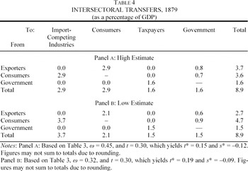
Table 4 presents an intersectoral transfer matrix that records the implied income transfers among five groups—import-competing producers, exporters, consumers, taxpayers, and the government—as a result of the tariff policy in 1879. The redistribution of income is calculated under the assumption of that the policy does not change total income and results are presented for the high and low estimates of the incidence parameter.²⁶

These results indicate that trade protection was responsible for reshuffling almost 9 percent of GDP between various agents in the economy. The implicit export tax accompanying the policy of import protection imposed a cost on exporters—measured as ωt*q_X / (1 − ω)— that ranged from 2.7 percent to 3.7 percent of GDP, depending on the high or low estimate of ω. Meanwhile, the tariff forced consumers to pay between 3.6 and 4.7 percent of GDP in terms of higher prices on importables, with 2.9 to 3.7 percent of GDP going to import-competing producers (t*q_M) and about 0.7 percent of GDP going to the government (t*m) in customs duties. Turning to the beneficiaries, import-competing industries gained 3.2 to 3.7 percent of GDP from consumers, while consumers gained the equivalent of about 2.2 percent of GDP at the expense of exporters by virtue of the lower prices of exportables. The government collected a total of about 1.6 percent of GDP in customs revenue, which—by assumption—was returned directly to taxpayers.

The most interesting question addressed by the transfer matrix is whether consumers benefited or lost from protection. Consumers gain from the lower domestic price of exportables (by the amount ω t*c_X / (1 − ω)) but lose from the higher domestic price of importables (by the amount t*c_M). This gives rise to the “neoclassical ambiguity” of the standard specific factors trade model wherein the change in the real wage as a result of the tariff hinges on the weights of goods in the consumption bundle.²⁷

In this case, the condition for consumers to gain from protection is ω > c_M / (c_M + c_X), i.e., when the incidence parameter is greater than the share of importables in the consumption of tradeables. Thus, consumers stand a chance of gaining from tariffs when domestic consumption of exportables is large.

The results here indicate that consumers lost income as a result of protection, but not a substantial amount. As the Table 4 indicates, consumers gained between 2.1 and 2.9 percent of GDP at the expense of exporters but paid 2.9 to 3.7 percent of GDP to import-competing producers (about 0.8 percent of GDP sent to the government in the form of tariff revenue is presumed to be returned to all consumers in a lump-sum payment). Thus, tariff protection cost consumers on net less than 1 percent of GDP. The reason import duties did not put a huge burden on consumers is that about 40 percent of consumption expenditures were devoted to food, and food accounted for more than half of U.S. exports in the mid-1880s. (After cotton, breadstuffs and meat were the largest categories of U.S. exports.) Although these products were important exports, most domestic production was consumed at home; for example, about three-quarters of the wheat crop was for domestic consumption. About 20 percent of consumer expenditures went to clothing, the major importable in the consumption bundle, and another 10 percent was devoted to tobacco manufactures and alcohol, both of which were imported to some degree.²⁸

Thus, as Table 4 indicates, the consumption of importables as a share of GDP exceeded that of exportables, but consumer spending was not highly skewed toward expenditures on importables.²⁹

Even if the net effect of protection on consumers was negative, consumers-cum-taxpayers could have gained from protection on the assumption that all the revenues from import duties (some of which are paid by exporters, not just consumers) were returned to consumers as a lump-sum rebate or exchanged for lower domestic taxes financing public goods.³⁰

Consumers-cum-taxpayers gain whenever the shift parameter exceeds the share of production of importables in the total production of tradeables, i.e., ω > q_M / (q_M + q_X), a condition that does not quite hold. Table 4 indicates that consumers lost 4.1 percent of GDP as a result of protection but gained 3.9 in government transfers, amounting to a net loss of just 0.2 percent of GDP. Thus, the overall effect of tariff protection on consumers as taxpayers was roughly neutral.

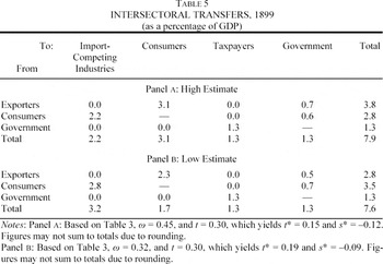
Table 5 presents the intersectoral transfer matrix for the year 1899. Due to structural changes in the economy, including the greater export orientation of U.S. manufacturers, the magnitude of the transfers in 1899 declined by a full percentage point of GDP compared with 1879. The implicit tax on exporters was roughly the same magnitude of GDP, but the transfers to import-competing industries fell from about 3.5 percent of GDP in 1879 to about 2.7 percent of GDP in 1899. Because of the declining transfers to import-competing industries and the bias in the structure of consumption toward exportables, consumers may have gained by protection in 1899 instead of losing as they had in 1879. However, the gain was very slight, only about 0.1 to 0.3 percent of GDP. Consumers-cum-taxpayers gained somewhat more from the policy of protection.

If the impact of tariffs on consumers as a broad class (and not in their role as producers) was roughly neutral by 1899, it would have been difficult to mobilize them to oppose the policy. In fact, in the 1888 presidential election fought largely over the tariff issue, the voting electorate was closely divided but slightly in favor of the tariff-reform candidate. The incumbent Democratic president, Grover Cleveland, who wanted to reduce tariff rates, received 48.6 percent of the vote, while his protariff Republican rival, Benjamin Harrison, received 47.8 percent of the vote. However, the geographic distribution of these votes ensured that Harrison won the electoral college by 233 to 168 and thus became president.³¹

The extremely close popular vote could be interpreted as indicating that the electorate was equally divided on the tariff question, consistent with the distributional effects here on consumers.

As a check on the results in Tables 4 and 5, we can use other data to assess the validity of the magnitude of the transfers reported here. The most transparent transfer is from the government to taxpayers. In 1879, the federal government collected $137 million in customs revenue, about 1.4 percent of nominal GDP, and in 1899 the government collected $206 million in customs revenue, about 1.1 percent of nominal GDP.³²

These figures are close to the 1.5 percent of GDP and 1.3 percent of GDP indicated in the calculations for those two years.

One important qualification suggests that these results may overstate the amount of redistribution brought about by the late-nineteenth-century tariffs. The magnitude of these transfers would be reduced if import tariffs significantly improved the terms of trade of the United States. It is unlikely that the estimates of the incidence parameter would be affected by tariff-induced terms-of-trade effects.³³

But if the United States was a large country, a major tariff change would not pass through to import prices on a one-for-one basis as assumed in these calculations. For example, the imposition of a 30 percent average tariff would not increase the relative price of importables by 30 percent, but by some fraction of that amount depending upon how much the tariff reduced the price of imports. Unfortunately, there is little evidence available on the ability of the United States to influence its terms of trade through policy measures.

AN ANTEBELLUM COMPARISON

Although this article has focused on the impact of the tariff in the late-nineteenth-century United States, this framework can also be used to shed some light on the antebellum period. Given the sharp political conflicts between the North and the South over tariff policy, the connections between the tariff and income distribution prior to the Civil War has long been of interest to economic historians. Clayne Pope, John James, and Harley all employed computable general equilibrium models of varying degrees of sophistication to examine the impact of the tariff prior to the Civil War (specifically, in 1859, in the cases of James and Harley).³⁴

The framework of net protection provides a much simpler, but also much less detailed, approach to the questions posed in those models.³⁵ Two key differences promise to make the results dissimilar to those for the late nineteenth century. First, the incidence parameter ω should be higher in the antebellum period. As ω also represents the degree of substitutability between traded and nontraded goods, a value closer to one than to zero implies somewhat more substitutability between importables and nontradeables than between exportables and nontradeables. In the antebellum period, exports consisted largely of cotton and tobacco produced on Southern plantations and other traditional goods (i.e., raw material or natural-resource-intensive primary products), which are typically less substitutable with nontradeables than are importables and nontradeables.³⁶ Second, the structure of the antebellum U.S. economy was quite different from that in the late nineteenth century. Although exports and imports as a percent of GDP were comparable, production of exportables (agriculture) was a larger and production of importables (manufactures) was a smaller part of the economy.

The results for the antebellum period will be presented very briefly. Export and import prices are from Douglass North, the money stock is from Peter Temin, the GDP deflator is taken from Johnston and Williamson, and the consumer price index is from David and Solar.³⁷

Like the findings in the previous section, the three variables—log(P_M / P_X) and log(P_N / P_X) using either the GDP deflator or the CPI—are nonstationary in levels but are stationary in first differences for the period 1815 to 1860. (These results are not reported.) Like the postbellum period, the levels regressions suggest that log(P_N / P_X) and log(P_M / P_X) are not cointegrated and hence those regression results are not consistent.

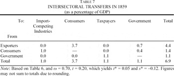
In the first-difference regressions, both the regressors and the residuals are stationary. In the first-difference estimate of equation 5′, the point estimates of ω are 0.65 (with a standard error of 0.06) using the GDP deflator and 0.78 (with a standard error of 0.08) using the consumer price index. Taking a rough estimate of ω as 0.70 along with an average tariff on all imports of 20 percent in late 1850s, equation 2′ indicates that this tariff would push up the price of nontradeables by 14 percent. This implies that the net protection given to import-competing producers (manufacturing) was just 5 percent and the effective tax on exporters (agriculture) was 12 percent. The higher estimate of ω implies a large impact on the price of nontraded goods and reaffirms Southerner complaints that the burden of the tariff was largely shifted onto Southern exporters through higher prices of importables and nontraded goods.

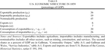
Table 6 presents the structure of the economy in 1859 and Table 7 presents the implied transfers.³⁸

Three differences stand out in comparison to the late-nineteenth-century period. First, the magnitude of the total transfers was smaller in the antebellum period, owing to the lower average tariff (after the early 1830s). Second, despite the lower tariff, transfers from exporters were greater in the antebellum period than in the Gilded Age. The greater resources squeezed from exporters combined with a greater commodity and geographic concentration of those exporters in the South made the tariff even more controversial in the antebellum period. Third, unlike the later period, consumers in the antebellum period appear to gain from the tariff because domestic consumption of exportables (agriculture) was greater while consumption of importables (manufactures) was lower as a percentage of GDP.³⁹ These results may be somewhat misleading in that the major exportables were cotton and tobacco, and at least the former was not directly purchased by consumer households but by textile firms in the North.

The Table 7 results can be compared with those in Harley's general equilibrium calculations.⁴⁰

Perhaps because the categories are not exactly comparable, the similarity in the results is mixed. Harley finds a much smaller positive impact of the tariff on the price of nontraded goods, only about 3 to 6 percent, as opposed to the 14 percent here. He also estimates that labor as a whole lost a small amount (about 0.5 percent) from the tariff whereas a nontrivial gain to consumers is estimated here (about 2 percent of GDP). This difference may be due to the different assumptions about the consumption bundle, as households were not the direct consumers of exportables such as cotton. However, Harley's estimate of the tariff's burden on farmers and planters is close to that found here; he estimates a loss of about 2 to 3 percent of GDP for farmers and planters (exporters), and the results here indicate it is about 4 percent. His gains to capital (an import-competing factor) are only about 0.4 percent of GDP whereas here they amount to about 1 percent of GDP.⁴¹