





1. Introduction
Stochastic resonance (SR) has long been recognised as a hallmark of bistable nonlinear systems, where interaction of noise and weak periodic forcing results in a strongly enhanced periodic signal (Benzi, Sutera & Vulpiani Reference Benzi, Sutera and Vulpiani1981; Gammaitoni et al. Reference Gammaitoni, Hänggi, Jung and Marchesoni1998). This phenomenon has been observed in diverse fields, such as biology, where SR appears due to enhancement of weak sensory signals by noise (Douglass et al. Reference Douglass, Wilkens, Pantazelou and Moss1993), and climate science, where it explains periodic Ice Age cycles (Benzi et al. Reference Benzi, Sutera and Vulpiani1981). Recently, SR has been identified as a critical mechanism in fluid dynamics (Li & Steinberg Reference Li and Steinberg2024a ).
Here, we discover SR in a viscoelastic channel flow as a key ingredient driving chaotic flow under conditions of a chaotic streamwise velocity power spectrum
 $E_u(f)$
and in the presence of flat, white-noise-like spanwise velocity power spectrum
 $E_w(f)$
with low intensity elastic waves, taking place above the instability onset. This new pathway with SR occurs just above the elastic instability onset in a lower subrange of a transition flow regime, whereas SR disappears in a upper subrange of transition regime and, further on, in the elastic turbulence (ET) and drag reduction (DR) flow regimes, where the amplification mechanism of vorticity fluctuations by the elastic wave becomes effective (Li & Steinberg Reference Li and Steinberg2023a
).
The elastic waves are non-dispersive transverse waves revealed in viscoelastic parallel shear chaotic flows and driven by elastic stress. Experimental studies of low-inertia polymer solution channel flow have demonstrated that elastic waves (Varshney & Steinberg Reference Varshney and Steinberg2019; Jha & Steinberg Reference Jha and Steinberg2021; Shnapp & Steinberg Reference Shnapp and Steinberg2022; Li & Steinberg Reference Li and Steinberg2023b
), emerging above the elastic instability onset, defined by the critical Weissenberg number (
 $\textit{Wi}_c$
), play a central role in promoting chaotic flow. The Weissenberg number (
 $\textit{Wi}$
) is defined as
 $\textit{Wi}=\lambda \dot {\gamma }$
, where
 $\lambda$
is the longest relaxation time of the polymer solution and
 $\dot {\gamma }$
is the shear rate, and
 $\textit{Wi}_c$
is the critical
 $\textit{Wi}$
upon which instability happens. These waves amplify wall-normal vortex fluctuations through resonant energy transfer withdrawn from the main flow (Li & Steinberg Reference Li and Steinberg2023a
), whereas at
 $\textit{Wi}_c$
, the elastic wave intensity is insufficient to amplify vortex fluctuations, leaving an essential gap in understanding the transition to chaotic flow. Our findings demonstrate that SR fills this gap (Li & Steinberg Reference Li and Steinberg2024a
).
This mechanism highlights the crucial role of elastic waves in mediating energy transfer in elastic chaotic flow: elastic waves extract energy from the mean flow and subsequently transfer it to wall-normal vortex fluctuations (Li & Steinberg Reference Li and Steinberg2023a ). The intensity of elastic waves governs the resulting chaotic states from the upper sub-range of the transition, ET and DR flow regimes. Here, the transition regime is defined as the flow state occurring above the onset of elastic instability up to the onset of ET (Jha & Steinberg Reference Jha and Steinberg2021; Li & Steinberg Reference Li and Steinberg2023b ). These three chaotic flow regimes differ by an exponent value of a power-law decay of the velocity power spectrum: in ET steeper than -3, whereas in transition and DR regimes flatter than −3 (Li & Steinberg Reference Li and Steinberg2023a ,Reference Li and Steinberg b ).
Finite external perturbations, quantified as root-mean-square streamwise velocity fluctuations at the inlet (
 $u^{\prime}_{rms}(l/h=0)$
), seed a new resonance mechanism of promoting chaotic flow downstream , i.e. SR. Notably, at sufficiently large external perturbations, SR emerges exclusively within a lower subrange of the transition regime, where the root-mean-square velocity fluctuations (
 $u^{\prime}_{rms}(l/h)$
) decrease relative to their inlet values (Li & Steinberg Reference Li and Steinberg2024a
,Reference Li and Steinberg
b
). Here,
 $u'(t) = u(t) - u_{mean}$
represents the fluctuating component of the streamwise velocity, with
 $u(t)$
being the time-dependent velocity and
 $u_{mean}$
the mean velocity at the channel centre,
 $l/h$
is the ratio of the distance from the channel inlet (
 $l$
) to its height (
 $h$
). This discovery provides a new perspective on the continuous (supercritical) transition from laminar to chaotic flow, driven by finite external perturbations
 $u^{\prime}_{rms}(l/h = 0)$
(Li & Steinberg Reference Li and Steinberg2024a
,Reference Li and Steinberg
b
,Reference Li and Steinberg
c
).
The first indicator of SR in viscoelastic channel flow is the appearance of a sharp peak at the frequency below algebraic decay in the chaotic power spectrum of the streamwise velocity
 $E_u(f)$
(Li & Steinberg Reference Li and Steinberg2024a
). In a typical SR framework, a weak periodic modulation superimposed on a noise background is essential. The modulation source is attributed to nascent elastic waves, while the noise is provided by the white-noise spanwise velocity fluctuations. The presence of a weak elastic modulation is reflected in the spanwise velocity spectrum
 $E_w(f)$
, which exhibits a flat profile just above the elastic instability threshold
 $\textit{Wi}_c$
. However, when at the inlet (
 $l/h = 0$
), the noise intensity becomes too strong, SR does not appear at
 $l/h=22$
, the closest vicinity to the inlet we could reach, but meanwhile the elastic wave intensity is found to be sufficiently high to amplify the wall-normal vorticity fluctuation at
 $l/h=22$
(Li & Steinberg Reference Li and Steinberg2024a
,Reference Li and Steinberg
c
). Based on these observations, the three essential ingredients for SR in viscoelastic channel flow can be summarised as follows: (i) the emergence of a distinct resonance peak in
 $E_u(f)$
; (ii) a spanwise velocity signal that resembles white noise, indicated by a flat
 $E_w(f)$
; and (iii) a weak elastic wave amplitude, corresponding to the early stages of elastic wave development just beyond
 $\mathrm{Wi_c}$
(Li & Steinberg Reference Li and Steinberg2024a
,Reference Li and Steinberg
b
).
Actually, SR in viscoelastic channel flows shares similarities with classical SR, which appears in bistable systems (Benzi et al. Reference Benzi, Sutera and Vulpiani1981; Gammaitoni et al. Reference Gammaitoni, Hänggi, Jung and Marchesoni1998). In these systems, external white noise induces switching between two stable states in a double-well potential with a mean frequency depending on the height of the potential barrier and noise intensity. Then, SR is realised in bistable systems driven simultaneously by noise and a weak periodic signal. However, the results reveal a distinct phenomenon: SR in chaotic flows exhibits a resonance-like peak in the chaotic power spectrum of the streamwise velocity (
 $E_u$
), in the presence of a flat, white-noise-like
 $E_w$
. A weak elastic wave acts as the periodic signal driving this resonance. This behaviour is reminiscent of deterministic stochastic resonance (DSR), observed in chaotic deterministic dynamical systems driven by weak periodic modulation and white noise (Anishchenko et al. Reference Anishchenko, Neiman and Safanova1993, Reference Anishchenko, Neiman, Moss and Shimali nsky-Geier1999).
Thus, we present the first experimental observation of DSR occurring above
 $\textit{Wi}_c$
in the lower subrange of the transition regime in inertia-less polymer solution channel flow (Li & Steinberg Reference Li and Steinberg2024a
). In the lower subrange, SR dominates, with its peak intensity (
 $I_p$
) in
 $E_u$
being significantly larger than the elastic wave intensity (
 $I_{el}$
), which is orders of magnitude smaller than that in the upper subrange of the transition regime. At higher
 $\textit{Wi}$
, in the upper subrange of the transition regime, ET and DR flow regimes, SR disappears, and the white-noise power spectrum
 $E_w$
transforms into a chaotic spectrum, characterised by a power-law decay and a significantly larger elastic wave peak intensity (Li & Steinberg Reference Li and Steinberg2024a
,Reference Li and Steinberg
b
).
In this study, we investigate the occurrence of DSR in a inertia-less polymer solution channel flow, where the inlet perturbations are significantly smaller than those considered in previous studies. Specifically, the inlet perturbation
 $u^{\prime}_{rms}(l/h = 0)$
is an order of magnitude smaller than in prior studies (Li & Steinberg Reference Li and Steinberg2023a
,Reference Li and Steinberg
b
), resulting in a substantially higher
 $\textit{Wi}_c =350$
compared with the typical range from 120 up to 150 in two identical channels but with different numbers of small holes on the top plate: six versus two, respectively (Li & Steinberg Reference Li and Steinberg2023a
,Reference Li and Steinberg
b
). This set-up provides a unique opportunity to examine how the appearance and characteristics of SR are affected by such small external perturbations. Additionally, we aim to clarify the nature of the wave associated with the DSR peak in
 $E_u$
. In particular, we seek to determine the nature of SR oscillation, that is, whether it is transverse or longitudinal and propagating or standing. This question remains unresolved in the literature, as existing theoretical models of SR focus on oscillations in deterministic systems, where time is the sole variable (Anishchenko et al. Reference Anishchenko, Neiman and Safanova1993, Reference Anishchenko, Neiman, Moss and Shimali nsky-Geier1999). Consequently, the spatial properties of DSR in polymer solution flows could be resolved either experimentally or by numerical simulations. By addressing these issues, this work seeks to deepen our understanding of DSR, its role in the continuous transition from laminar to chaotic flow and the complex relationship between external perturbations and chaotic dynamics.
2. Experimental set-up and methods
The experiments were performed in a linear channel with dimensions
 $L \times h \times W = 450 \times 0.5 \times 3.5$
mm
 $^3$
, where
 $L$
is the total length of the linear channel and
 $W$
is the channel width, as illustrated in figure 1. The channel was fabricated using transparent acrylic glass. The bottom plate was precision machined to ensure a uniform cross-section and a smooth inlet configuration, while the top plate was drilled with a circular opening to accommodate an O-ring seal. The top and bottom plates were assembled using a stainless steel frame, secured with screws, and sealed with an appropriately sized O-ring. Two channel configurations were tested: one without holes and another with two small holes (0.5 mm in diameter) on the top plate. In the latter configuration, one hole was located upstream at
 $l/h = -80$
, far from the inlet, and the other downstream near the outlet. The longitudinal and transverse coordinates of the channel were designated as
 $x$
and
 $z$
, respectively, with the origin (
 $x$
,
 $z$
) = (0, 0) defined at the start of the straight channel. The inlet geometry tapered over a 50 mm length in the
 $x$
direction, narrowing from 5.5 to 0.5 mm in the
 $y$
direction and from 5 to 3.5 mm in the
 $z$
direction.
Schematic of the experimental set-up. The polymer solution is stored in a large stainless steel vessel and driven by compressed nitrogen gas, controlled by pressure regulators. The solution flows through a straight channel with a smoothed inlet. The solution exiting the outlet is collected in a beaker placed on a balance. Two holes, located outside the inlet and outlet, are used to reduce potential external disturbances and measure pressure fluctuations. The balance measures the flow discharge rate. Seeded tracers are illuminated by a thin laser sheet in the
 $x{-}z$
plane at the centre of the channel, and a high-speed camera is used for image acquisition.

The working fluid is a dilute polymer solution of high molecular weight polyacrylamide (Polysciences,
 $M_w = 18$
MDa) at a concentration of 80 ppm (
 $c/c^* \approx 0.4$
), where
 $c^* \approx 200$
ppm is the overlap concentration (Liu, Jun & Steinberg Reference Liu, Jun and Steinberg2009). The solvent is a water–sucrose mixture with a sugar weight fraction of 64 %. The solution properties are as follows: the density,
 $\rho = 1320$
kg m−
 $^3$
; the solvent viscosity,
 $\eta _s = 0.13$
Pa
 $\cdot$
s; and the total solution viscosity,
 $\eta = 0.17$
Pa
 $\cdot$
s. The ratio of solvent viscosity to total solution viscosity is
 $\eta _s / (\eta _s + \eta _p) = 0.765$
, where
 $\eta _p$
is the polymer contribution to the viscosity. The longest polymer relaxation time,
 $\lambda = 13$
s, was obtained using the stress relaxation method (Liu et al. Reference Liu, Jun and Steinberg2009).
The fluid is driven by nitrogen gas at pressures up to 120 psi. The instantaneous fluid discharge,
 $m(t)$
, is measured using a PC-interfaced balance (BPS-1000-C2-V2, MRC). The time-averaged fluid discharge rate,
 $Q = \langle \Delta m / \Delta t \rangle$
, is used to calculate the average velocity,
 $U = Q / (\rho W h)$
. The Weissenberg number,
 $\textit{Wi} = \lambda U / h$
, and the Reynolds number,
 $\textit{Re} = \rho U h / \eta$
, vary in the ranges of (100, 6000) and (0.015, 0.9), respectively. The resulting
 $\mathrm{El} = \textit{Wi} / \textit{Re} = \lambda \eta / \rho h^2 = 6.7 \times 10^3$
.
The flow field at various positions
 $l/h$
was analysed using particle image velocimetry (PIV). The PIV set-up utilised 3.2
 $\unicode{x03BC} \mathrm{m}$
latex particle tracers at a concentration of approximately 1 % w/w (Thermo Scientific), illuminated by a laser sheet with a thickness of approximately 50
 $\unicode{x03BC} \mathrm{m}$
in the central channel plane (
 $x{-}z$
plane). A high-speed camera (Mini WX100 FASTCAM, Photron) with high spatial resolution captured images of tracer pairs at frame rates ranging from 2000 to 20 000 fps. The velocity components
 $u(x, z, t)$
and
 $w(x, z, t)$
in the two-dimensional
 $x{-}z$
plane were obtained using the OpenPIV software (Liberzon et al. Reference Liberzon, Käufer, Bauer, Vennemann and Zimmer2020). Data were recorded for approximately
 $\mathcal{O}(30)$
minutes, or
 $\mathcal{O}(100\lambda )$
, at each
 $\textit{Wi}$
to ensure sufficient statistics. For velocity fluctuations shown in figures 2, 3, 4, 5 and 6, spatial averaging was performed over narrow windows with a resolution of 256 (
 $x$
)
 $\times$
96 (
 $z$
) pixels
 $^2$
using a 4x objective, which is served as a single-point velocity measurement at the channel centre. This spatial averaging method, combined with sufficiently long-time statistics, ensures the accuracy of the measurements. The temporally averaged velocity in these narrow regions is denoted as
 $U_{\mathrm{mean}}$
for normalisation. For the velocity profiles in figure 9(a), (b) and (d), and velocity cross-correlation in figure 9(c), the window resolutions were chosen as minimal slits. These velocities were averaged within narrow regions: spanning the
 $x$
direction with a resolution of 256 (
 $x$
) pixels. The PIV window size was 32
 $\times$
32 pixels
 $^2$
, with a 50 % overlap and a search window size of 200 %.
3. Results
The main difference between the current channel and those used in previous experiments (Li & Steinberg Reference Li and Steinberg2023a
,Reference Li and Steinberg
b
, Reference Li and Steinberg2024a
,Reference Li and Steinberg
b
) is the carefully smoothed and tapered inlet, designed to minimise external flow disturbances (Li & Steinberg Reference Li and Steinberg2024c
), similar to the set-up in Shnapp & Steinberg (Reference Shnapp and Steinberg2022). The instability occurs under conditions of negligible inertia but high elasticity, characterised by a critical Reynolds number
 $\textit{Re}_c \approx 0.05$
and
 $\textit{Wi}_c = 350 \pm 20$
.
Left column: streamwise velocity fluctuations (
 $u^{\prime}_{p}(t)$
) partially averaged over 100 neighbouring points, plotted versus time (
 $t$
). Right column: corresponding streamwise velocity power spectra (
 $E_u$
) (without averaging), plotted against normalised frequencies (
 $\lambda f$
) in lin–log scale for low-frequency ranges at various downstream positions (
 $l/h$
) and
 $\textit{Wi}$
. Panels show (a) and (b)
 $l/h=40$
at
 $\textit{Wi}=525, 1078$
; (c) and (d)
 $l/h=90$
at
 $\textit{Wi}=525, 1120, 2850, 5710$
; (e) and (f)
 $l/h=635$
at
 $\textit{Wi}=550, 1150, 2760, 5510$
, covering the transition, ET and DR flow regimes. Measurements are made by PIV in the centre of the x–z plane.

3.1. Streamwise periodic sharp spikes
Upon reaching instability, streamwise velocity fluctuations (
 $u'(t)$
) at the channel centre exhibit periodic sharp spikes within the chaotic flow. As shown in figure 2, the first column and ten rows, labelled as (a, c and e), present the temporal evolution of the streamwise velocity fluctuations (
 $u^{\prime}_p(t)$
) averaged over 100 consecutive points over a 1 second period, measured at three downstream positions:
 $l/h =$
40, 90 and 635, and for various
 $\textit{Wi}$
values across the transition, ET and DR regimes. For comparison, the original temporal evolution of
 $u'(t)$
without averaging at
 $l/h = 90$
and 635 for several
 $\textit{Wi}$
values in the ET and DR regimes is shown in figure 3. Although noisy, periodic velocity fluctuations are clearly visible. Remarkably, five time series of
 $u'(z,t)$
, presented at
 $z/W$
positions located symmetrically around the centre at
 $z/W=0$
, at the highest value of
 $Wi=5217$
in DR and
 $l/h=500$
, show surprising agreement in their frequencies.
The first key observation in figure 2 is the variation in periodic spikes associated with SR at different downstream positions. At
 $l/h = 40$
, these spikes – and hence SR – appear only at two values of
 $\textit{Wi}$
: 525 and 1078, within the lower subrange of the transition flow regime (Li & Steinberg Reference Li and Steinberg2024c
). In contrast, at
 $l/h = 90$
and 635, SR spikes are observed across all three flow regimes. In the five rightmost rows (b, d and f),
 $E_u$
are plotted against the frequency normalised by the longest relaxation time (
 $\lambda f$
) in logarithm–linear (log–lin) coordinates for the same positions and
 $\textit{Wi}$
values as in figure 2(a, c and e). These power spectra reveal sharp, high-intensity SR peaks. As observed, at
 $l/h = 40$
, the SR peaks occur exclusively in the lower subrange of the transition flow regime near
 $\textit{Wi}_c$
, while at
 $l/h = 90$
and 635, SR peaks are present across all three flow regimes. These
 $E_u$
data are also presented in logarithm–logarithm (log–log) coordinates in figure 4.
Temporal evolution of stream-wise velocity fluctuations
 $u'(t)$
. (a)
 $Wi = 2850$
and
 $l/h = 90$
, (b)
 $Wi = 2760$
and
 $l/h = 635$
, and (c)
 $Wi = 5710$
and
 $l/h = 90$
show short time series demonstrating periodic noisy spikes. (d) Five time series of
 $u'(z,t)$
at five fixed
 $z/W$
values at
 $Wi = 5217$
and
 $l/h = 500$
.

Streamwise velocity power spectra
 $E_u$
versus
 $\lambda f$
in log–log coordinates at
 $l/h = 40, 90, 635$
. For each
 $l/h$
value, data are shown at four different
 $Wi$
values in three flow regimes. The decay regions of
 $E_u$
are fitted by power-law relationships, represented by dashed lines, with corresponding exponent values indicated.

In figure 5(a, b and c), we present plots of probability density function (PDF) of the streamwise velocity,
 $P(u'/ u^{\prime}_{rms})$
, measured at the centre of the
 $x$
–
 $z$
channel midplane, for the same three downstream positions and
 $\textit{Wi}$
values. As reported previously (Li & Steinberg Reference Li and Steinberg2024a
), for
 $\textit{Wi} \lt \textit{Wi}_c$
, the PDFs follow a Gaussian distribution. However, for
 $\textit{Wi} \gt \textit{Wi}_c$
, within the lower subrange of the transition regime, the PDFs deviate from Gaussian behaviour, with the deviation becoming more pronounced as
 $\textit{Wi}$
increases – especially for negative
 $u'/u^{\prime}_{rms}$
values corresponding to negative spikes. This deviation from Gaussian, associated with SR, disappears at
 $\textit{Wi} \gt 300$
in the upper subrange of the transition regime, and further in the ET and DR regimes (Li & Steinberg Reference Li and Steinberg2024a
,Reference Li and Steinberg
b
), where the negative tail becomes exponential, a characteristic feature of chaotic flows (Groisman & Steinberg Reference Groisman and Steinberg2004). While deviations from Gaussianity are also evident in the present data (figure 5
a, b and c), these deviations are less pronounced compared with those reported earlier (Li & Steinberg Reference Li and Steinberg2024a
), particularly at
 $l/h =$
90 and 635, as the result of an order of magnitude smaller noise intensity at the inlet. To quantify the deviation from Gaussian, we plot the ratio of the PDFs at
 $\textit{Wi} \gt \textit{Wi}_c$
to the Gaussian PDF as a function of
 $u'/u^{\prime}_{rms}$
in figure 5(d, e and f).
Upper row: PDFs of normalised streamwise velocity fluctuations (
 $P(u'/u_{rms})$
) Lower row: ratio between
 $P(u'/u_{rms})$
and the Gaussian distribution at the channel centre for three downstream positions (
 $l/h$
) and varying
 $\textit{Wi}$
. Panels show (a) and (d)
 $l/h = 40$
at
 $\textit{Wi} = 525, 1078, 2760, 5620$
; (b) and (e)
 $l/h = 90$
at
 $\textit{Wi} = 525, 1120, 2850, 5710$
; (c) and (f)
 $l/h = 635$
at
 $\textit{Wi} = 550, 1150, 3760, 5510$
, covering the transition, ET and DR flow regimes. Gaussian PDFs for
 $\textit{Wi} \lt \textit{Wi}_c = 350$
are included for each
 $l/h$
as a reference. Arrows in (a) and (d) indicate increasing
 $\textit{Wi}$
.

3.2. Spanwise flat white noise
In figure 6(a, b and c), we present
 $E_w$
as a function of
 $\lambda f$
in log–log coordinates at
 $l/h =$
40, 90 and 635, for
 $\textit{Wi}$
values above
 $\textit{Wi}_c$
in the three flow regimes. Except for
 $l/h = 40$
at
 $\textit{Wi} = 2760$
and 5620 in the ET and DR flow regimes, the spectra are flat, indicating a white-noise power spectrum similar to the behaviour observed at
 $\textit{Wi} \lt \textit{Wi}_c$
. In these instances, elastic wave peaks are either not noticeable or several orders of magnitude smaller than those at
 $l/h = 40$
and higher
 $\textit{Wi}$
values.
Power spectra of spanwise velocity (
 $E_w$
) versus normalised frequency (
 $\lambda f$
) in log–log scale for three downstream positions (
 $l/h$
) at different
 $\textit{Wi}$
values. Panels (a), (b) and (c) correspond to
 $l/h = 40, 90, 635$
, respectively, with four values in the transition, ET and DR flow regimes, consistent with figures 1 and 2 in the main text. Large elastic wave peaks are clearly noticeable only at
 $l/h=40$
in ET and DR flow regimes. In contrast, at all other
 $l/h$
and
 $\textit{Wi}$
values, the spanwise power spectra,
 $E_w$
, are flat, and elastic wave peaks are not distinguishable.

Range of SR occurrence in
 $\textit{Wi}-l/h$
coordinates. For
 $l/h \geqslant 90$
, SR peaks are observed across all three flow regimes. Green squares represent cases without SR, while red circles denote cases with SR detected. The dashed line indicates the boundary between cases with and without SR.

3.3. Range of SR appearance
The appearance of SR, characterised by streamwise low-frequency velocity spikes and spanwise flat white noise, depends on both control parameters
 $l/h$
and
 $\textit{Wi}$
. Figure 7 reveals an intriguing result: the range of SR occurrence is much broader at smaller external perturbations compared with flows with larger inlet noise, where SR is restricted to the lower subrange of the transition regime, just above
 $\textit{Wi}_c$
(Li & Steinberg Reference Li and Steinberg2024b
). As shown by Li & Steinberg (Reference Li and Steinberg2024b
), three factors are critical for SR to emerge as a function of
 $\textit{Wi}$
and
 $u^{\prime}_{rms}(l/h)$
: (i) a flat, white-noise power spectrum
 $E_w$
, (ii) a chaotic power spectrum
 $E_u$
and (iii) low-intensity elastic waves
 $I_{el}$
(see figure 8
b). The phase diagram for
 $\textit{Wi}$
and
 $l/h$
coordinates in figure 7 demonstrates that SR appears in all three flow regimes for
 $l/h \geqslant 90$
, for much smaller external perturbations compared with previous studies, where SR was confined to the lower subrange of the transition regime (Li & Steinberg Reference Li and Steinberg2024a
,Reference Li and Steinberg
b
). The SR is also observed at
 $l/h = 16$
for
 $\textit{Wi}$
= 515 and 1070, and at
 $l/h = 40$
for
 $\textit{Wi} = 525$
and 1078, both only in the lower range of the transition flow regime (see figure 7 and figure 8).
(a) Values of
 $\lambda f_p$
and
 $\lambda f_{el}$
versus
 $Wi$
at all
 $l/h$
values in three flow regimes. (b) Values of
 $I_p$
and
 $I_{el}$
versus
 $Wi$
at all
 $l/h$
values in three flow regimes. The quantities
 $\lambda f_p$
and
 $\lambda f_{el}$
are fitted to the function
 $A \times (Wi / Wi_c - 1)^\gamma$
, with exponents
 $\gamma = 0.45 \pm 0.05$
for
 $\lambda f_p$
and
 $\gamma = 0.5 \pm 0.05$
for
 $\lambda f_{el}$
. The dashed line in the lower plot of (b) represents the resolution limit of
 $I_{el}$
.

3.4. Spatial properties of periodic spikes
Finally, to investigate the spatial properties of the periodic spikes, figure 9 presents two experimental approaches to determine whether SR represents either standing or propagating wave in the
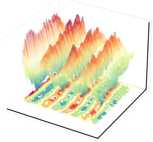
 $x{-}z$
plane and transverse or longitudinal waves. As shown in figure 9(a,b), SR is shown by space–time plots of the streamwise velocity fluctuations,
 $u'(z,t)$
, with uniform amplitude in the
 $z$
-direction. The first method, described by Varshney & Steinberg (Reference Varshney and Steinberg2019), involves calculating the SR propagation velocity in the
 $z$
-direction
 $c_{p}$
using the cross-correlation function
 $C(\Delta z, \tau )$
of
 $u'(z,t)$
, shown in the insets of figure 9(c), for
 $\textit{Wi} = 5217$
,
 $l/h = 500$
(left) and
 $\textit{Wi} = 1850$
,
 $l/h = 70$
(right). By varying
 $\Delta z$
, the spatial separation between two points in the
 $z$
-direction, and measuring the corresponding time shift
 $\tau$
of the
 $C(\Delta z, \tau )$
peak, the SR propagation velocity in the z-direction
 $c_{p} = \Delta z / \tau$
is found to be approximately zero inside sufficiently large error bars (figure 9
c). The second method is based on reconstruction of a three-dimensional (3-D) SR image of
 $u'(z,t)$
as a function of
 $z$
and
 $t$
(figure 9
d, at
 $\textit{Wi} = 5217$
,
 $l/h = 500$
). Since the wave profile is parallel to the
 $z$
-axis, SR propagation velocity in
 $z$
-direction is nearly zero, as shown above. On the other hand, in figure 9(d),
 $u'(z,t)$
, located in the x–zplane in the
 $x$
-direction, demonstrates oscillations in the
 $x$
-direction, being evidence of their longitudinal nature. The problem whether SR is propagating or standing waves should be resolved separately. The temporal dynamics of SR oscillations presented by
 $u'(z,t)$
is shown in the Supplementary Movie.
Characterisation of SR in 2-D and 3-D space–time plots. (a,b) Space–time plots of the streamwise velocity fluctuations (
 $u'(z,t)$
) under band-pass filters [0.21, 0.27] and [0.1, 0.12], at
 $\textit{Wi} = 5217$
,
 $l/h = 500$
and
 $\textit{Wi} = 1850$
,
 $l/h = 70$
, respectively. (c) Cross-correlation function
 $C(\Delta z, \tau )$
of
 $u'(z, t)$
at
 $\textit{Wi} = 5217$
,
 $l/h = 500$
(left) and
 $\textit{Wi} = 1850$
,
 $l/h = 70$
(right), shown in insets. Here,
 $C(\Delta z, \tau )$
is used to determine the SR propagation velocity (
 $c_{p} = \Delta z/\tau$
) by varying
 $\Delta z$
and measuring the time shift
 $\tau$
of the
 $C(\Delta z, \tau )$
peak. (d) A 3-D presentation of SR at
 $\textit{Wi} = 5217$
and
 $l/h = 500$
, with
 $u'(z, t)$
plotted against
 $z$
and
 $t$
in colour.

4. Discussion
In our experiments, we observe DSR manifesting in low-inertia polymer solution channel flows as a resonance-like peak in
 $E_u$
. This peak arises due to the cooperative interaction between a chaotic
 $E_u$
, white-noise-like
 $E_w$
and low-intensity elastic waves above
 $\textit{Wi}_c$
. With the inlet external perturbations (
 $u^{\prime}_{rms}(l/h=0)$
) reduced by an order of magnitude, figure 7 provides clear evidence that DSR occurs at
 $\textit{Wi}\gt \textit{Wi}_c$
over the channel length from
 $l/h\geqslant 90$
, in all three flow regimes: transition, ET and DR. These flow regimes are well established and characterised by distinct dependencies of the normalised friction factor, pressure fluctuations and both streamwise and spanwise velocity fluctuations measured at
 $l/h = 320$
as a function of
 $\textit{Wi}$
(Li & Steinberg Reference Li and Steinberg2024c
). We observe a distinct phenomenon from those with different inlet perturbations (Pan et al. Reference Pan, Morozov, Wagner and Arratia2013; Qin et al. Reference Qin, Salipante, Hudson and Arratia2019; Jha & Steinberg Reference Jha and Steinberg2021; Shnapp & Steinberg Reference Shnapp and Steinberg2022; Li & Steinberg Reference Li and Steinberg2023a
,Reference Li and Steinberg
b
): the temporal evolution of
 $u^{\prime}_p (t)$
shows almost periodic spikes, which are characterised by sharp SR peaks in
 $E_u$
, as shown in figure 2 and figure 8.
As presented in Li & Steinberg (Reference Li and Steinberg2024a
), both flat white-noise-like power spectra
 $E_u$
and
 $E_w$
exist below
 $\textit{Wi}_c=150$
(figure. 7), where also spikes are absent (figure 4 in Li & Steinberg Reference Li and Steinberg2024a
). While at
 $\textit{Wi}\gt \textit{Wi}_c$
,
 $E_u$
becomes chaotic and spikes appear but
 $E_w$
remains flat in the lower subrange of the transition flow regime. Notably, in the channel with the smoothed inlet and with
 $\textit{Wi}_c=350$
, in figure 5 of Li & Steinberg (Reference Li and Steinberg2024c
) and figure 6 and figure 4 in the current paper,
 $E_w$
remains flat at
 $l/h=0$
and higher depending on the
 $Wi$
values and whether
 $E_u$
stays flat close to the inlet and becomes chaotic at
 $l/h\gt 0$
and
 $\textit{Wi}\gt \textit{Wi}_c$
.
The emergence and persistence of DSR are particularly striking when compared with flows with larger external perturbations. It is crucial that the appearance and persistence of DSR up to the largest
 $\textit{Wi}$
– enabled by the presence of flat white-noise-like
 $E_w$
–represents a breakthrough in the understanding of the stochastic nature of the mechanism to promote a sustained chaotic flow above
 $\textit{Wi}_c$
up to the largest
 $\textit{Wi}$
value, when the elastic wave intensity is insufficient to amplify wall-normal vortex fluctuations. This unexpected striking difference of the DSR occurrence range compared with flows at much larger perturbations at the inlet is directly linked to the appearance range of a flat, white-noise-like power spectrum of the spanwise velocity fluctuations. The transformation of
 $E_w$
thus serves as the critical factor delineating the DSR regime from subsequent chaotic flow states. While previous studies identified DSR only in a narrow range near
 $\textit{Wi}_c$
(Li & Steinberg Reference Li and Steinberg2024a
,Reference Li and Steinberg
b
), we demonstrate that the persistence of a white-noise spectrum for
 $E_w$
is the key ingredient driving DSR far beyond the onset of elastic instability. As mentioned above, the puzzle of whether DSR represents a propagating or standing wave could only be resolved experimentally, especially at sufficiently low noise levels. The theoretical models currently used to explain DSR are based on deterministic dynamical chaotic systems where time is the only variable, and they do not consider spatial variables, thus suggesting oscillations without clearly distinguishing between standing and propagating or transverse and longitudinal waves (Anishchenko et al. Reference Anishchenko, Neiman and Safanova1993, Reference Anishchenko, Neiman, Moss and Shimali nsky-Geier1999). Thus, a deterministic dynamical chaotic systems with predicted DSR are not suitable to consider spatial DSR features. Here, in our experiments, we provide the first experimental proof to our knowledge that SR manifests as either a standing or propagating longitudinal wave in the
 $x$
-direction, with a uniform amplitude of
 $u'(z,t)$
in the
 $z$
-direction, shown in the space–time plots in figure 9(a) at
 $\textit{Wi} = 1850$
,
 $l/h = 70$
and figure 9(b) at
 $\textit{Wi} = 5217$
,
 $l/h = 500$
. The second approach involves measuring the wave propagation velocity
 $c_p$
in the z-direction for different values of
 $\textit{Wi}$
by calculating
 $C(\Delta z, \tau )$
of
 $u'(z,t)$
. By varying
 $\Delta z$
and measuring the time shift
 $\tau$
of the peak in
 $C(\Delta z, \tau )$
, the propagation velocity
 $c_{p} = \Delta z / \tau$
in the
 $z$
direction is found to be zero within the measurement errors (figure 9
c).
These results constitute a major step forward in understanding the chaotic transition in polymer solution channel flows. By highlighting the persistence of DSR under minimal perturbation conditions and its dependence on white-noise-like spanwise velocity fluctuations, we provide a robust mechanism that connects the onset and evolution of chaos in viscoelastic fluid flows. This work not only resolves longstanding questions about the transition to chaos, but also broadens the applicability of DSR as a framework for analysing complex dynamical systems, opening the door for future numerical simulations to further validate these results.
Supplementary movie
Supplementary movie is available at https://doi.org/10.1017/jfm.2025.10309.
Acknowledgements
The authors thank G. Han and R. Baron for their help in setting up the experimental set-up. Y.L. is grateful for the assistance of R. Min on data post-processing and the valuable discussion with Professors A. Zhang and H. Zhang.
Funding
This project has received funding from National of Science Foundation of China (No.12472255). The Scientific Research Innovation Capability Support Project for Young Faculty (No. ZYGXQNJSKYCXNLZCXM-O1) and the Fundamental Research funds for the Central Universities (No. 3072025CFJ0102).
Declaration of interests
The authors report no conflict of interest.
Author contributions
Y.L. and V.S. designed the experiment. Y.L. performed the experiments. Y.L. and V.S. analysed the data and wrote the manuscript.



