1. Introduction
Stress-release processes are a class of point processes, the first of which were self-correcting processes [Reference Isham and Westcott7]. Intuitively, a process is self-correcting if the occurrence of past points inhibits the occurrence of future points. The stress-release processes are a generalization of self-correcting processes and were introduced in a series of papers by Vere-Jones and others [Reference Zheng and Vere-Jones24, Reference Zheng and Vere-Jones25] as well as extensions to coupled stress-release processes [Reference Liu, Vere-Jones, Ma, Shi and Zhuang11, Reference Lu, Harte and Bebbington12, Reference Shi, Liu, Vere-Jones, Zhuang and Ma18] and further developments [Reference Bebbington and Harte1, Reference Bebbington and Harte2].
In this study we work with a generalization of the stress-release process which includes an exogenous point process term whose values upon arrival are modeled by a positive real-valued random variable. We call our model the extrinsic stress-release processes.
We present a new formula for the law of the joint inter-arrival times for extrinsic stress-release processes. As a natural consequence, an exact simulation algorithm is then proposed which gives an alternative method to generating sample paths relative to standard methods [Reference Lewis and Shedler9]. Our exact simulation algorithm naturally extends the results of [Reference Wang, Vere-Jones and Zheng22] as a special case. The extension of our model is motivated by the influence of exogenous geophysical data on earthquake occurrence (see e.g. [Reference Ogata15] and [Reference Zhuang and Ma26]). Point process models of this kind are typically used to describe the evolution of stochastic phenomena in earthquake modeling, and it is important to be able to simulate them for reliable predictions of damage due to a range of earthquake scenarios. Thinning algorithms [Reference Ogata14] have been successfully employed to simulate a wide range of point processes, such as inhomogeneous point processes (see [Reference Daley and Vere-Jones5, pages 270–271] and [Reference Zammit-Mangion, Dewar, Kadirkamanathan and Sanguinetti23]), or Hawkes processes [Reference Veen and Schoenberg19]. Indeed, the same idea can be applied to the generalized stress-release process proposed here. In this paper, simulation of the extrinsic stress-release process by our exact algorithm will be compared with the standard thinning algorithm.
Finally, we present the infinitesimal generator for extrinsic stress-release processes. This generator is intimately linked to the martingale problem, which is used to characterize the weak solutions of partial integro-differential equations [Reference Liptser and Shiryaev10], and it allows us to derive the theoretical reciprocal moments of the intensity function. In Section 6 these reciprocal moments are used to demonstrate the correctness of our simulation algorithms. Basic notions and results in stochastic calculus are taken as prerequisites throughout the present text (see e.g. [Reference Protter17]).
2. Extrinsic stress-release model
At the base of everything is some filtered probability space
 $(\Omega,\mathcal{F},\mathbb{F},\mathbb{P})$
. We assume that
 $\mathcal{F}_0$
is trivial, and the filtration
 $\mathbb{F} \,{:}\,{\raise-1.5pt{=}}\, (\mathcal{F}_t)_{t\geq 0}$
fulfills the usual conditions and is generated by a point process
 $N(\cdot)$
on
 $\mathbb{R}_{+}$
where
 $0 < T_1 < T_2 < \cdots$
denote the occurrence times of the events. Let
 $N_t = \sharp\{T_i \,:\, 0 < T_i \le t\}$
be the number of the occurrence points in the time interval (0, t] with
 $N_0=0$
. Furthermore, we let
 $N^{\prime}_t = \sharp\{T^{\prime}_j \,:\, 0 < T^{\prime}_j \le t\}$
be a Poisson process on
 $\mathbb{R}_{+}$
, with arrival times
 $0 <T^{\prime}_1 < T^{\prime}_2< \cdots$
endowed with intensity
 $\rho$
, which is independent of
 $N_t$
, with
 $N^{\prime}_0=0$
.
Definition 2.1. The proposed extrinsic stress-release process
 $N(\cdot)$
is a point process on
 $\mathbb{R}_+$
with conditional intensity function given by
 \begin{align}\lambda_t \,{:}\,{\raise-1.5pt{=}}\, \lambda(t\mid \mathcal{F}_t) = \lambda_0\exp(\beta t - S_t - S^{\prime}_t),\,\quad t\geq 0,\end{align}
where
 $S_t=\sum_{i\,:\, T_i< t} X_i$
and
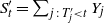 $S^{\prime}_t=\sum_{j\,:\, T^{\prime}_j < t} Y_j$
are the compound point process and compound Poisson process, respectively. The
 $X_i$
and
 $Y_j$
are i.i.d. positive random variables, with distribution functions
 $F_X$
and
 $F_Y$
respectively, and the stress accumulation rate is the constant
 $\beta>0$
.
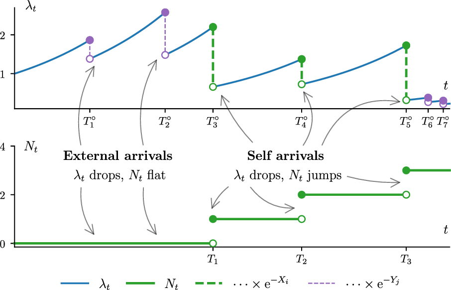
Between jumps,
 $\lambda_t$
increases exponentially with a positive rate of
 $\beta>0$
. Jumps are downward multiplicative factors of size
 $\textrm{e}^{-X_i} < 1$
for a self-arrival at time
 $T_i$
, or of size
 $\textrm{e}^{-Y_j} < 1$
for an external arrival at time
 $T^{\prime}_j$
. When a self-arrival occurs at time
 $T_i$
,
 $N_t$
increases by one, hence
 $(N_t, \lambda_t)$
is a Markov process. Instead of separating the self-arrivals of
 $N_t$
and the external arrivals of
 $N^{\prime}_t$
, it is sometimes convenient to consider all the arrivals indiscriminately. As such, we label the kth arrival as
 $T^\circ_k$
, and it can correspond either to some self-arrival
 $T_i$
or some external arrival
 $T^{\prime}_j$
. See Figure 1 for an example realization of the extrinsic stress-release process, with the effects of the self-arrivals and external arrivals on the conditional intensity function
 $\lambda_t$
highlighted.
An example realization of an extrinsic stress-release process, with
 $\lambda_0 = 1$
,
 $\beta = 1.5$
,
 $\rho = 2$
, and
 $X_i \sim \mathsf{Exp}(1)$
and
 $Y_j \sim \mathsf{Exp}(2)$
. Note that N is càdlàg while
 $\lambda$
is càglàd.

Remark 2.1. Our proposed extrinsic stress-release process differs slightly from the coupled stress-release model of [Reference Liu, Vere-Jones, Ma, Shi and Zhuang11]. Their equivalent of
 $X_i$
and
 $Y_j$
from Definition 2.1 are not unobserved random variables: they are deterministic functions of the observed earthquake magnitudes. In our proposed model, we allow for these quantities to take any i.i.d. random variables that are positive and unobserved, so our formulation generalizes theirs. Unlike ours, they allow for model parameters c and
 $c^{\prime}$
in the exponent of equation (2.1) of the form
 \begin{equation*}-c S_t - c^{\prime} S^{\prime}_t ,\end{equation*}
where c and
 $c^{\prime}$
can take either negative or positive values, thereby allowing for both damping and excitation. We only consider the inhibitory regime, i.e.
 $c=c^{\prime}=1$
, so in this case their formulation for general c and
 $c^{\prime}$
subsumes ours. In either formulation, little or no work has appeared on exact simulation strategies for the coupled stress-release model. We also add some new aspects to the computation of explicit generators, facilitating moment computations. For other theoretical and stationary moment calculations without the exogenous term S
′, see [Reference Borovkov and Vere-Jones3], [Reference Ogata and Vere-Jones16], [Reference Vere-Jones20], and [Reference Vere-Jones and Ogata21].
3. The law of joint inter-arrival times
In this section we present the explicit law of the joint inter-arrival times for extrinsic stress-release processes. This terminology, ‘joint inter-arrival time’, refers to the time between each of
 $T^\circ_k$
arrivals (defined in Section 2). Itô’s formula [Reference Jacod and Shiryaev8] splits
 $\lambda_t$
into continuous and jump components:
 \begin{equation*}\lambda_t = \lambda_0 + \int_0^t\beta\lambda_s \textrm{d}{s} + \sum_{i \,:\, T_i \le t} \lambda_{T_i} \left(\textrm{e}^{-X_i}-1\right) + \sum_{j \,:\, T^{\prime}_j \le t} \lambda_{T^{\prime}_j} \left(\textrm{e}^{-Y_j}-1\right) .\end{equation*}
Between consecutive jumps the
 $\lambda$
process evolves according its continuous part. In particular, conditioned on
 $T^\circ_k$
and
 $\lambda_{T^{\circ+}_k}$
, we have
 \begin{equation} \lambda_t = \lambda_{T^{\circ+}_k} \exp(\beta(t-T^\circ_k)) \quad \text{for } t \in (T^\circ_k, T^\circ_{k+1}).\end{equation}
The intensity of the
 $T^\circ_k$
arrivals is the combination of the
 $T_i$
and
 $T^{\prime}_j$
arrival intensities
 $\lambda_t + \rho$
. Let the kth joint inter-arrival time be denoted by
 $\tau_k \,{:}\,{\raise-1.5pt{=}}\, T^\circ_k-T^\circ_{k-1}$
with cumulative density function
 $F_{\tau_{k}}$
. With (3.1), we can simplify the point process relation
 \begin{align} F_{\tau_{k+1}}(t)= 1 - \exp\biggl( {-} \int_{0^+}^t (\lambda_{T^\circ_k + s} + \rho) \textrm{d}{s} \biggr)= 1 - \exp\biggl( {-} \frac{\lambda_{T^{\circ+}_k}}{\beta} (\textrm{e}^{\beta t}-1) \biggr) \textrm{e}^{-\rho t} ,\end{align}
which is the law of the joint inter-arrival times.
4. Simulation methods
The law of the joint inter-arrival times in (3.2) can be used to derive a simulation method for extrinsic stress-release processes. To simulate we need to (i) generate
 $T^\circ_k$
joint inter-arrival times, and (ii) be able to attribute each arrival as being either a self-arrival from
 $N_t$
or an external arrival from
 $N^{\prime}_t$
. By the inverse probability integral transform, we have
 \begin{equation*}\tau_{k+1} \overset{\mathcal{D}}{=} F_{\tau_{k+1}}^{-1}(U),\quad U\sim \mathsf{U}[0,1],\end{equation*}
where
 $\overset{\mathcal{D}}{=}$
denotes equality in distribution. The inverse
 $F_{\tau_{k+1}}^{-1}$
does have an analytic solution (which is somewhat rare) in terms of the Lambert W-function, so we can generate joint inter-arrival times by the inverse transform method. However, the Lambert W-function is relatively slow in many software packages, and this calculation does not perform the second attribution step. A faster alternative, which solves both problems at once, is to use the composition method.
4.1. Exact simulation of stress-release model
The composition method [Reference Devroye6, Section VI.2.3] simulates
 $\tau_{k+1}$
from two simpler independent random variables
 $\tau^{(1)}_{k+1}$
and
 $\tau^{(2)}_{k+1}$
by taking
 \begin{equation*}\tau_{k+1} \overset{\mathcal{D}}{=} \tau^{(1)}_{k+1} \wedge \tau^{(2)}_{k+1},\end{equation*}
where the notation
 $\tau^{(1)}_{k+1} \wedge \tau^{(2)}_{k+1}$
is simply shorthand for
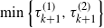 $\min\left\{ \tau^{(1)}_{k+1}, \tau^{(2)}_{k+1} \right\}$
. One way to satisfy this relation is to choose
 \begin{equation*}\mathbb{P}\left(\tau^{(1)}_{k+1}>s\right) = \exp\left({-} \lambda_{T^{\circ+}_k} \beta^{-1} \left(\textrm{e}^{\beta s}-1\right)\right)\quad\text{and}\quad\mathbb{P}\left(\tau^{(2)}_{k+1}>s\right)=\textrm{e}^{-\rho s},\end{equation*}
so
 \begin{align}\tau^{(1)}_{k+1} & \overset{\mathcal{D}}{=} \frac{1}{\beta}\log\biggl(1-\frac{\beta}{\lambda_{T^\circ_k}}\log(U_1)\biggr),\quad\tau^{(2)}_{k+1} \overset{\mathcal{D}}{=} -\frac{1}{\rho}\log(U_2),\quad U_1,U_2\sim \textsf{U}[0,1].\end{align}
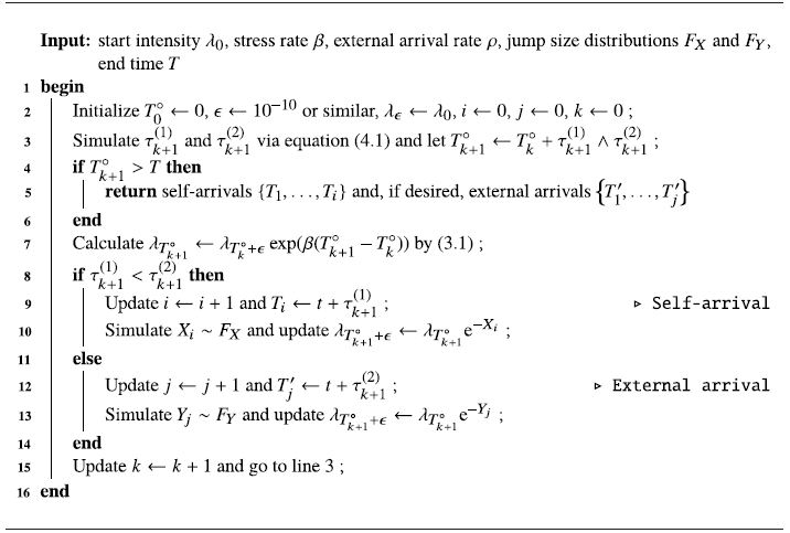
This is the key step in the composition algorithm, presented in full in Algorithm 1.1.
Generate an extrinsic stress-release process by composition.

4.2. Simulation by thinning
Extrinsic stress-release processes can also be simulated via the thinning algorithm. The basic idea in this method is to generate a point process that has more arrivals than the model dictates, then probabilistically remove the excess points. The result can be computationally inefficient, and we compare the runtime of the thinning and composition simulation methods in Section 6.
The first step in thethinning algorithm is to generate the
 $N^{\prime}_t$
and
 $S^{\prime}_t$
processes. The self-arrivals are then generated conditional on these external arrivals. Each self-arrival is generated sequentially and requires a local upper bound on the intensity process. If we know
 $S^{\prime}_t$
for all
 $t \in \mathbb{R}_+$
, we obviously have
 \begin{equation*} \lambda_t \leq \lambda_0\exp(\beta t - S^{\prime}_t),\,\quad t\in\mathbb{R}_+, \end{equation*}
though as t increases this becomes an extremely loose bound. However, if we also know the process
 $S_t$
up until time
 $\tau$
, then
 \begin{align}\overline{\lambda}_{t \mid \tau} \,{:}\,{\raise-1.5pt{=}}\, \lambda_0\exp(\beta t - S_{t \wedge \tau} - S^{\prime}_t),\,\quad t\in\mathbb{R}_+,\end{align}
is a much tighter upper bound on the intensity, at least for
 $t \in (\tau, \tau+\Delta)$
for moderately small
 $\Delta$
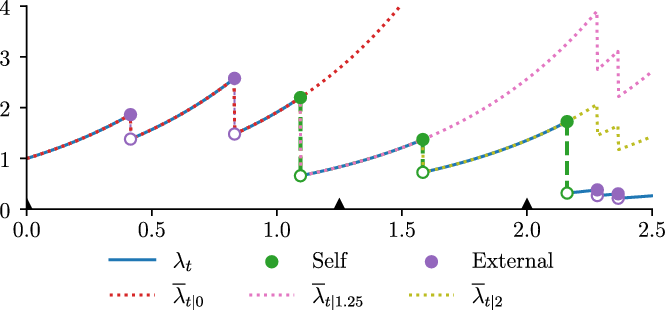
. Figure 2 shows some example realizations of (4.2).
Example
 $\overline{\lambda}_{t \mid \tau}$
upper bounds on the intensity function
 $\lambda_t$
. This is the same realization of the generalized stress-release process from Figure 1.

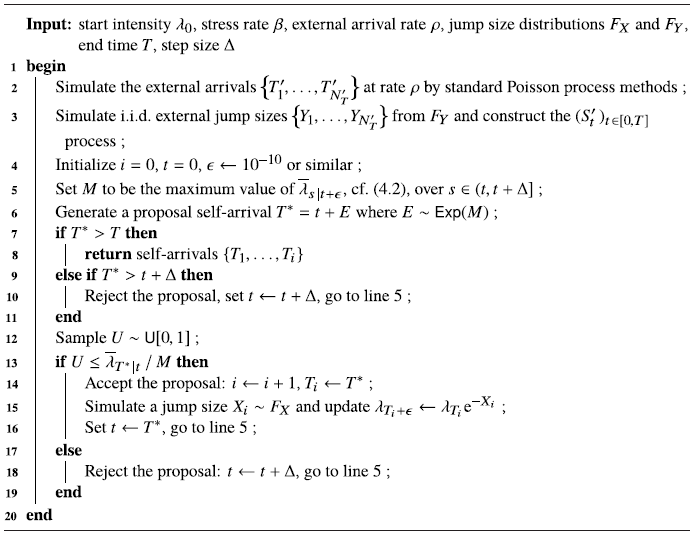
With this definition, we can describe the thinning algorithm for the generalized stress-release process in Algorithm 1.2. In particular, line 5 of the algorithm uses (4.2) to find an upper bound of
 $\lambda_t$
over a small region
 $t \in (\tau, \tau+\Delta]$
; these maximum values are not too tedious to find, as they occur either at the end time
 $\tau+\Delta$
or at one of the external arrival times
 $T^{\prime}_j$
that arrives inside the region.
Generate an extrinsic stress-release process by thinning.

5. The generator
In this section we derive theexplicit form of the infinitesimal generator for our process. With this we are able to find reciprocal moments, which are then used to confirm the validity of our simulation algorithm.
5.1. Constructing the infinitesimal generator
Let us introduce the integro-differential operator
 $\mathcal{L}^{\textrm{sr}}$
of our extrinsic stress-release process
 $(\lambda_t,N_t,t)$
, which acts on a function
 $f(\lambda,n,t)$
within its domain
 $\Omega(\mathcal{L}^{\textrm{sr}})$
as follows:
 \begin{align}\mathcal{L}^{\textrm{sr}} f & \,{:}\,{\raise-1.5pt{=}}\, \frac{\partial f}{\partial t} + \beta\lambda \frac{\partial f}{\partial t} + \lambda \int_{\mathbb{R}} [f(\lambda \textrm{e}^{-x},n+1,t)-f(\lambda,n,t)] \, F_X(\textrm{d}{x}) \notag \\
&\quad\, + \rho \int_{\mathbb{R}} [f(\lambda \textrm{e}^{-y},n,t)-f(\lambda,n,t)] \, F_Y(\textrm{d}{y}).\end{align}
From Propositions II.1.16 & II.1.15 in [Reference Jacod and Shiryaev8], the conditional intensity function in equation (2.1) can be recast as
 \begin{equation*}\lambda_t = \lambda_0\exp\biggl(\beta t - \int_0^t\int_{\mathbb{R}} x \mu(\textrm{d}{x}, \textrm{d}{s}) - \int_0^t\int_{\mathbb{R}} y \mu'(\textrm{d}{y}, \textrm{d}{s})\biggr),\end{equation*}
where
 $\mu$
and
 $\mu'$
are the jump measures associated with S and S
′, respectively. Their associated predictable compensators are
 $\nu(\textrm{d}{x}, \textrm{d}{t}) = F_X(\textrm{d}{x}) \lambda_t \textrm{d}{t}$
and
 $\nu'(\textrm{d}{y}, \textrm{d}{t}) = F_Y(\textrm{d}{y}) \rho \textrm{d}{t}$
. We now state the following result.
Proposition 5.1. Let the integro-differential operator for our stress-release process be defined as in equation (5.1). Then, for each
 $t\in\mathbb{R}_+$
, we obtain
 \begin{align*} \mathbb{E}[f(\lambda_t,N_t,t)] = f(0,N_0,\lambda_0) + \mathbb{E}\biggl[\int_0^t \mathcal{L}^{\textrm{sr}} f(\lambda_s,N_s,s) \textrm{d}{s}\biggr]\end{align*}
if the following f-integrability conditions hold:
 \begin{align}\mathbb{E}\biggl[\int_0^t \lambda_s \textrm{d}{s} \int_{\mathbb{R}} [f(\lambda_{s^+},N_s,s)-f(\lambda_s,N_{s^-},s)]^2 \, F_X(\textrm{d}{x}) \biggr]<\infty\end{align}
and
 \begin{align}\mathbb{E}\biggl[\int_0^t \rho \textrm{d}{s} \int_{\mathbb{R}} [f(\lambda_{s^+},N_s,s)-f(\lambda_s,N_{s^-},s)]^2 \, F_Y(\textrm{d}{y}) \biggr]<\infty .\end{align}
Moreover, f satisfies the following partial integro-differential equation:
 \begin{align}& \frac{\partial f}{\partial t} + \beta\lambda\frac{\partial f}{\partial\lambda} + \lambda \int_{\mathbb{R}}[f(\lambda \textrm{e}^{- x},n+1,t)-f(\lambda,n,t)] F_X(\textrm{d}{x}) \notag \\ & \quad\, +\rho\int_{\mathbb{R}}[f(\lambda \textrm{e}^{-y},n,t)-f(\lambda,n,t)] F_Y(\textrm{d}{y})=0.\end{align}
Proof. First note that
 $\lambda_t$
can be recast as
 \begin{equation*}\lambda_{t} = \lambda_0 + \int_0^t \beta\lambda_{s} \textrm{d}{s} + \int_0^t\int_{\mathbb{R}}\lambda_s(\textrm{e}^{- x}-1)\mu(\textrm{d}{x}, \textrm{d}{s})+ \int_0^t\int_{\mathbb{R}}\lambda_s(\textrm{e}^{- y}-1)\mu'(\textrm{d}{y}, \textrm{d}{s}).\end{equation*}
Invoking Itô’s formula (see [Reference Medvegyev13, Chapter VI]) on the arbitrary function
 $f(\lambda_t,N_t,t)$
yields
 \begin{align*}f(\lambda_t,N_t,t) & = f(\lambda_0,N_0,0) + \int_0^t \frac{\partial f}{\partial s} \textrm{d}{s} + \int_0^t \frac{\partial f}{\partial\lambda} \textrm{d}{\lambda_s^{c}} + \sum_{0<s\leq t} [f(\lambda_{s^+},N_s,s) - f(\lambda_s,N_{s^-},s)],\end{align*}
where
 $\lambda^c$
denotes the continuous part of the semimartingale. We can write
 \begin{align*}&\sum_{0<s\leq t}[f(\lambda_{s^+},N_s,s) - f(\lambda_s,N_{s^-},s)]\\ &\quad = \sum_{0<s\leq t}[f(\lambda_{s^+},N_s,s) - f(\lambda_s,N_{s^-},s)]\cdot\Delta N_s \\& \quad\quad\, + \sum_{0<s\leq t}[f(\lambda_{s^+},N_s,s) - f(\lambda_s,N_{s^-},s)]\cdot\Delta N^{\prime}_s \\&\quad = Q_t(f) + \int_0^t\int_{\mathbb{R}} [f(\lambda_{s^+},N_s,s) - f(\lambda_s,N_{s^-},s)]\,\nu(\textrm{d}{x}, \textrm{d}{s}) \\ & \quad\quad\, + Q^{\prime}_t(f) + \int_0^t\int_{\mathbb{R}} [f(\lambda_{s^+},N_s,s) - f(\lambda_s,N_{s^-},s)]\,\nu'(\textrm{d}{x}, \textrm{d}{s})\end{align*}
with
 $Q_{\cdot}(f)$
and
 $Q^{\prime}_{\cdot}(f)$
being processes defined by
 \begin{equation*}Q_{\cdot}(f) \,{:}\,{\raise-1.5pt{=}}\, \int_0^{\cdot} \int_{\mathbb{R}} [f(\lambda_{s^+},N_s,s) - f(\lambda_s,N_{s^-},s)](\mu-\nu)(\textrm{d}{x}, \textrm{d}{s})\end{equation*}
and
 \begin{equation*}Q^{\prime}_{\cdot}(f) \,{:}\,{\raise-1.5pt{=}}\, \int_0^{\cdot} \int_{\mathbb{R}} [f(\lambda_{s^+},N_s,s) - f(\lambda_s,N_{s^-},s)](\mu'-\nu')(\textrm{d}{x}, \textrm{d}{s}),\end{equation*}
respectively. The integrability conditions in equations (5.2) and (5.3) guarantee that Q(f) and Q
′(f) are square-integrable martingales [Reference Brémaud4, Theorem VIII of Chapter II]. Hence we conclude that the process
 $(f(\lambda_t,N_t,t))_{t\in\mathbb{R}_+}$
is a special semimartingale [Reference Protter17] which can be decomposed into a martingale and a predictable finite variation process
 \begin{align}f(\lambda_t,N_t,t)-f(\lambda_0,N_0,0) = Q_t(f) + Q^{\prime}_t(f)+\int_0^t \mathcal{L}^{\textrm{sr}} f(\lambda_s,N_s,s) \,{\textrm{d}{s}}.\end{align}
Since Q(f) and Q’(f) are square-integrable martingales, the process defined by
 \begin{align*} \biggl(f(\lambda_t,N_t,t)-f(\lambda_0,N_0,0)-\int_0^t \mathcal{L}^{\textrm{sr}} f(\lambda_s,N_s,s) \,{\textrm{d}{s}} \biggr)_{t\in\mathbb{R}_+}\end{align*}
is also a square-integrable martingale. Taking the expected value of both sides of equation (5.5) yields the result. For the subsequent expression, first define
 $T > t$
and
 $g_t \,{:}\,{\raise-1.5pt{=}}\, \mathbb{E}[h(\lambda_T,N_T,T)\mid t,\lambda_t=\lambda,N_t=n]$
for some function h such that g satisfies the g-integrability conditions (5.2) and (5.3). Then, by construction,
 $g_t$
is a martingale. By similar arguments, we see that
 $g-Q(g)-Q'({g})$
is a square-integrable martingale, but
 $g - Q(g)-Q'(g) = \int_0^\cdot \mathcal{L}^{\textrm{sr}} g \textrm{d}{s}$
is also a continuous process with finite variation. It must therefore be a continuous martingale with finite variation [Reference Jacod and Shiryaev8, Corollary I-3.16]; hence we must have
 $\mathcal{L}^{\textrm{sr}} g=0$
 $\mathbb{P}$
-almost surely, which yields the partial integro-differential equation in (5.4).
5.2. Reciprocal moments
Consistent with the observation in [Reference Vere-Jones and Ogata21], we are unable to find moments of
 $\lambda_t$
but we can find moments of its reciprocal. Throughout Sections 5.2 and 5.3 we assume that
 $\lambda_0 = 1$
, though the same arguments can be made in the general
 $\lambda_0$
case.
Lemma 5.1. Let
 $m_1^S \,{:}\,{\raise-1.5pt{=}}\, \int (\textrm{e}^{x}-1) \, F_X(\textrm{d}{x})$
and
 $m_1^E \,{:}\,{\raise-1.5pt{=}}\, \int (\textrm{e}^{y}-1) \, F_Y(\textrm{d}{y})$
. We assume that
 $\beta>\rho m_1^E$
and
 $\lambda_0 = 1$
. Then the expectation of
 $\lambda^{-1}_t$
is given by
 \begin{align}\mathbb{E}[{\lambda^{-1}_t}] = \textrm{e}^{-\psi_1 t} + \frac{m_1^S}{\psi_1}(1-\textrm{e}^{-\psi_1 t}),\end{align}
where
 $\psi_1 \,{:}\,{\raise-1.5pt{=}}\, \beta-\rho m_1^E$
.
Proof. From Proposition 5.1, we have for
 $f\in\Omega(\mathcal{L}^{\textrm{sr}})$
that
 \begin{equation*} f(\lambda_t,N_t,t) - f(\lambda_0,N_0,0) - \int \mathcal{L}^{\textrm{sr}} f(\lambda_s,N_s,s) \textrm{d}{s} \end{equation*}
is an
 $\mathcal{F}$
-martingale. Setting
 $f=\lambda^{-1}$
in the generator yields
 \begin{equation*}\mathcal{L}^{\textrm{sr}} (\lambda^{-1}) = -{\beta}{\lambda^{-1}} + m_1^S + {\rho}{\lambda^{-1}} m_1^E\end{equation*}
and
 \begin{equation*}\mathbb{E}\biggl[\lambda^{-1}_t-\lambda^{-1}_0-\int_0^t \mathcal{L}^{\textrm{sr}} (\lambda^{-1}_s) \textrm{d}{s} \biggr]=0.\end{equation*}
Differentiating
 $\theta_1(t) \,{:}\,{\raise-1.5pt{=}}\, \mathbb{E}[{\lambda^{-1}_t}]$
with respect to t yields the non-linear inhomogeneous ODE
 \begin{equation*}\theta^{\prime}_1 + \psi_1 \theta_1=m_1^S,\quad\theta_1(0)=1,\end{equation*}
whose solution is given in equation (5.6).
By a similar token, and setting
 $f=\lambda^{-2}$
, we state the following.
Lemma 5.2. Let
 \begin{equation*} m_2^S \,{:}\,{\raise-1.5pt{=}}\, \int \big(\textrm{e}^{2x}-1\big) \, F_X(\textrm{d}{x}), \quad m_2^E \,{:}\,{\raise-1.5pt{=}}\, \int \big(\textrm{e}^{2x}-1\big) \, F_Y(\textrm{d}{y}). \end{equation*}
We assume that
 $\beta>\rho m_1^E$
,
 $2 \beta > \rho m_2^E$
, and
 $\lambda_0 = 1$
. Then the expectation of
 $\lambda^{-2}_t$
is given by
 \begin{align}\mathbb{E}[{\lambda^{-2}_t}]\,{=}\,\textrm{e}^{-\psi_2 t} \,{+}\, m^S_2 \biggl\{\frac{\textrm{e}^{-\psi_1 t} \,{-}\, \textrm{e}^{-\psi_2 t}}{\psi_2 - \psi_1} \,{+}\,\frac{m_1^S}{\psi_1} \biggl[\biggl(\frac{1}{\psi_2} \,{-}\, \frac{\textrm{e}^{-\psi _1 t}}{\psi_2 - \psi_1}\biggr) -\textrm{e}^{-\psi_2 t} \biggl(\frac{1}{\psi_2} - \frac{1}{\psi_2 - \psi_1}\biggr)\!\biggr]\!\biggr\},\end{align}
where
 $\psi_2 \,{:}\,{\raise-1.5pt{=}}\, 2\beta - \rho m_2^E$
.
We end this section by giving some recursive relationships related to the inverse moments of our process. Let
 $\mathbb{N}$
be the set of natural numbers and let
 $k\in\mathbb{N}$
,
 $m_k^S \,{:}\,{\raise-1.5pt{=}}\, \int (\textrm{e}^{kx}-1) \, F_X(\textrm{d}{x})$
,
 $m_k^E \,{:}\,{\raise-1.5pt{=}}\, \int (\textrm{e}^{ky}-1) \, F_Y(\textrm{d}{y})$
, and
 $\psi_k\,{:}\,{\raise-1.5pt{=}}\, k\beta-\rho m^E_k$
. We further assume that
 $k\beta>\rho m^E_k$
. Then the generator for the function
 $f=\lambda^{-k}$
is readily computed as follows:
 \begin{align*}\mathcal{L}^{\textrm{sr}}(\lambda^{-k})=m_k^S\lambda^{k-1} - \psi_k\lambda^{k}.\end{align*}
By the martingale property we have that
 \begin{align}\mathbb{E}\biggl[\lambda^{-k}_t-\lambda^{-k}_0-\int_0^t \mathcal{L}^{\textrm{sr}} (\lambda^{-k}_s) \textrm{d}{s} \biggr]=0.\end{align}
Define the quantity
 $\theta_k(t) \,{:}\,{\raise-1.5pt{=}}\, \mathbb{E}[{\lambda^{-k}_t}]$
, and differentiating equation (5.8) with respect to t, we arrive at the recursive non-linear inhomogeneous ODE
 \begin{align*}\theta^{\prime}_k(t)+\psi_k \theta_k(t) = m^S_k\theta_{k-1}(t) ,\end{align*}
where
 $\theta_0\equiv 1$
, which can be solved in a recursive fashion to obtain further reciprocal moments.
5.3. Covariance process
We provide an expression for the mean of the product of two reciprocals of intensities for our process. This can be used to compute the covariance process. For
 $s<t$
, it holds true that
 \begin{align}\mathbb{E}\left[\lambda_t^{-1}\lambda_s^{-1}\right] & =\mathbb{E}\left[\mathbb{E}\left[\lambda_t^{-1}\lambda_s^{-1}\mid \lambda_s^{-1}\right]\right]\nonumber \\& =\textrm{e}^{-\psi_1 (t-s)}\mathbb{E}\left[\lambda_s^{-2}\right]+\frac{m^S_1}{\psi_1}(1-\textrm{e}^{-\psi_1(t-s)})\mathbb{E}\left[\lambda^{-1}_s\right].\end{align}
To see why this is true, note that the inner expectation can be computed as follows:
 \begin{align*}\mathbb{E}\left[\lambda_t^{-1}\lambda_s^{-1}|\lambda_s^{-1}\right] & =\lambda_s^{-1}\mathbb{E}\left[\lambda_t^{-1}|\lambda_s^{-1}\right]=\lambda_s^{-2}\textrm{e}^{-\psi_1 (t-s)}+\lambda^{-1}_s\frac{m^S_1}{\psi_1}\left(1-\textrm{e}^{-\psi_1(t-s)}\right).\end{align*}
Therefore, for
 $s < t$
, we have
 \begin{align*}\mathbb{C}\textrm{ov}\left(\lambda_s^{-1}, \lambda_t^{-1}\right)&= \mathbb{E}\left[\lambda_t^{-1}\lambda_s^{-1}\right] - \mathbb{E}\left[\lambda_t^{-1} \right] \mathbb{E}\left[\lambda_s^{-1} \right] \\&= \textrm{e}^{-\psi_1 (t-s)}\mathbb{E}\left[\lambda_s^{-2}\right]+\frac{m^S_1}{\psi_1}\left(1-\textrm{e}^{-\psi_1(t-s)}\right)\mathbb{E}\left[\lambda^{-1}_s\right] - \mathbb{E}\left[\lambda_t^{-1} \right] \mathbb{E}\left[\lambda_s^{-1} \right],\end{align*}
where the remaining expectations are given by (5.6) and (5.7). Furthermore, when we set
 $S^{\prime}=0$
in equation (2.1), we retrieve the covariance results in [Reference Borovkov and Vere-Jones3, Theorem 2, page 317] upon substituting the results of Lemmas 5.1 and 5.2 to get an expression for equation (5.9) and subsequently subtracting the quantity
 $\mathbb{E}[\lambda^{-1}_t]\cdot\mathbb{E}[\lambda^{-1}_s]$
.
6. Numerical results
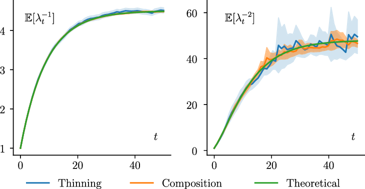
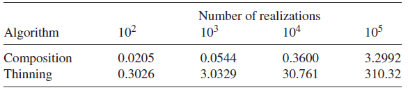
To confirm that the simulation algorithms of Section 4 agree with the reciprocal moments derived in Section 5, we compare the first reciprocal moments given by the theory to Monte Carlo estimates. The results are given in Figure 3. The theory and the simulated values agree nicely. This example is also used to illustrate the speed benefits to the composition simulation method over the thinning method. In particular, Table 1 shows how long the two algorithms took to generate a fixed number of realizations of the extrinsic stress-release process. The difference in performance can be explained by (i) the fact that the composition method is easily vectorized while thinning is not, and (ii) the thinning algorithm is inherently inefficient as it intentionally generates too many points and discards a possibly large fraction of them.
First reciprocal moments
 $\mathbb{E}\big[{\lambda^{-1}_t}\big]$
and second reciprocal moments
 $\mathbb{E}\big[{\lambda^{-2}_t}\big]$
for
 $t \in [0, 50]$
of an extrinsic stress-release process with
 $\lambda_0 = 1$
,
 $\beta = 0.25$
,
 $\rho = 1.25$
, and
 $X_i \sim \mathsf{Exp}(3)$
and
 $Y_j \sim \mathsf{Exp}(10)$
. The theoretical values, given by (5.6) and (5.7), are compared with crude Monte Carlo estimates using the two simulation methods from Section 4. Both simulation methods were allocated the same amount of computation time (55–60 seconds); as such, Algorithm 1.1 generated
 $375\,000$
sample paths of
 $\lambda_t$
, whereas Algorithm 1.2 generated
 $25\,000$
. The shaded regions indicate the 95% confidence intervals of the Monte Carlo estimates.

Comparison of runtime (in seconds) to simulate a number of realizations of the extrinsic stress-release process until time
 $T = 100$
using Algorithms 1.1 and 1.2. The fastest time of three attempts is recorded. A grid search is performed to select the optimal step size
 $\Delta = 1.86$
for Algorithm 1.2 (this search is not included in the runtimes). The specification of the process (
 $\lambda_0$
,
 $\beta$
,
 $\rho$
, etc.) is the same as in Figure 3.

7. Concluding remarks
In this article we have introduced a straightforward but computationally efficient way of simulating exactly for a class of generalized stress-release process. The idea stems from the observation that between contiguous jumps at points in time, the process satisfies the continuous part of the semimartingale and is thus governed by an ordinary differential equation. This permits us to derive an expression for the distribution between events. The end result is that we are able to sidestep the need to resort to thinning algorithms for the simulation of this class of point processes.
The explicit form of the infinitesimal generator for the extrinsic stress-release process is given. Theoretical reciprocal moments are derived which are then used to establish the validity of our simulation algorithms.
We envisage that the approach outlined in this paper extends naturally to the general coupled stress release models, i.e. the linked stress-release model [Reference Bebbington and Harte1, Reference Bebbington and Harte2] with appropriate structures satisfying the martingale generators. Ongoing work is investigating such a problem.
Acknowledgements
Young Lee is grateful to Professors Angelos Dassios and Louis Chen for inspiring discussions. An anonymous referee is thanked for his/her careful reading of an earlier version of the paper leading to a significant improvement of the presentation.
Funding information
Patrick J. Laub conducted this research within the DAMI – Data Analytics and Models for Insurance – Chair under the aegis of the Fondation du Risque, a joint initiative by UCBL and BNP Paribas Cardif. Hongbiao Zhao would like to acknowledge the financial support from the National Natural Science Foundation of China (#71401147) and the research fund provided by the Innovative Research Team of Shanghai University of Finance and Economics (#2020110930) and Shanghai Institute of International Finance and Economics.
Competing interests
There were no competing interests to declare which arose during the preparation or publication process of this article.
Data
The Python code used to generate the numerical results is available at https://github.com/Pat-Laub/exact-simulation-of-extrinsic-stress-release-processes.