1. Introduction
As spanwise wall oscillation has been shown to attain a drag reduction (
 ${\mathcal{D}}{\mathcal{R}}$
) as high as 40 % (Jung, Mangiavacchi & Akhavan Reference Jung, Mangiavacchi and Akhavan1992), this type of flow control techniques have attracted considerable attention among other methods (Karniadakis & Choi Reference Karniadakis and Choi2003). The main aim of such control methods is to reduce the skin-friction drag (Choi, DeBisschop & Clayton Reference Choi, DeBisschop and Clayton1998; Dhanak & Si Reference Dhanak and Si1999; Bandyopadhyay Reference Bandyopadhyay2006), which is of paramount importance in many engineering applications. One prominent application of flow control is in the transport industry, in particular, the air transport, in which a significant reduction of drag corresponds to large fuel savings and a lower level of
 $\text{CO}_{2}$
emissions (Bieler et al.
Reference Bieler, Abbas, Chiaramonte and Sawyers2006; Spalart & McLean Reference Spalart and McLean2011). For these high-Reynolds-number situations, an understanding of the Reynolds number effect is crucial, as a knowledge of the drag reduction achievable at a cruise condition gives an important insight into the applicability of the control method.
Wall oscillation can be defined by two parameters: the maximum wall velocity,
 $A$
, and the time period of the oscillation,
 $T$
,
 $$\begin{eqnarray}w(x,y=0,z,t)=A\sin ({\it\omega}t),\end{eqnarray}$$
where
 ${\it\omega}=2{\rm\pi}/T$
is the angular frequency. In this study,
 $x,y$
and
 $z$
denote the streamwise, wall-normal and spanwise directions, respectively. The effects of these parameters on drag reduction at
 $\mathit{Re}_{{\it\tau}}=200$
has been examined with a parametric study by Quadrio & Ricco (Reference Quadrio and Ricco2004). The friction Reynolds number of the turbulent channel flow is defined as
 $\mathit{Re}_{{\it\tau}}=u_{{\it\tau}}h/{\it\nu}$
, where
 $u_{{\it\tau}}$
is the friction velocity,
 $h$
is the channel half-width, and
 ${\it\nu}$
is the kinematic viscosity of the fluid. (The friction velocity is defined as
 $u_{{\it\tau}}\equiv \sqrt{{\it\tau}_{w}/{\it\rho}}$
, where
 ${\it\tau}_{w}$
is the wall shear stress and
 ${\it\rho}$
is the density of the fluid.) Quadrio & Ricco (Reference Quadrio and Ricco2004) observed that, for any given
 $T^{+}$
, the drag reduction increases with
 $A^{+}$
, but the rate of increase diminishes as
 $A^{+}$
becomes large. In this study, the superscript
 $+$
represents wall units using
 $u_{{\it\tau}}$
and
 ${\it\nu}$
. An optimal value of
 $T^{+}$
is found in the range
 $100\leqslant T^{+}\leqslant 125$
, as discussed by Karniadakis & Choi (Reference Karniadakis and Choi2003), which can give the maximum drag reduction of around 40 %, whilst a drag increase is achieved when a large time period (
 $T^{+}=1000$
) is employed at
 $\mathit{Re}_{{\it\tau}}=200$
(Jung et al.
Reference Jung, Mangiavacchi and Akhavan1992).
The temporal wall oscillation case can be converted to a purely spatial one, involving a streamwise dependant, sinusoidal wave of spanwise velocity (Viotti, Quadrio & Luchini Reference Viotti, Quadrio and Luchini2009). The stationary wave can be defined by the maximum wall velocity,
 $A$
, and the streamwise wave length of the oscillation,
 ${\it\lambda}$
,
 $$\begin{eqnarray}w(x,y=0,z,t)=A\sin ({\it\kappa}_{x}x),\end{eqnarray}$$
where
 ${\it\kappa}_{x}=2{\rm\pi}/{\it\lambda}$
is the spatial wavenumber. As the near-wall structures move along the wave, a similar effect to that of wall oscillation is experienced; in fact, the stationary wave was found to be more effective than the wall oscillation for any given
 $A^{+}$
. For example, for
 $A^{+}=12$
, the optimal wall oscillation (with
 $T^{+}=100$
) resulted in a drag reduction of 33 % while the stationary wave produced a drag reduction of 45 %. The optimal wavelength of the forcing is in the range
 $1000\leqslant {\it\lambda}^{+}\leqslant 1250$
, in which the stationary wave produces a significantly larger drag reduction compared with the wall oscillation case. The optimal of the wall oscillation and stationary wave cases are related by a convection velocity
 $U_{c}^{+}\approx 10$
. Recently, the effectiveness of stationary wave was confirmed by Skote (Reference Skote2013) for the boundary-layer flow.
A general form of the streamwise travelling waves incorporates both the wall oscillation and stationary wave into one wall control technique (Quadrio, Ricco & Viotti Reference Quadrio, Ricco and Viotti2009). This flow control method is applied in the form
 $$\begin{eqnarray}w(x,y=0,z,t)=A\sin ({\it\kappa}_{x}x-{\it\omega}t).\end{eqnarray}$$
These travelling waves are equivalent to the temporal and spatial cases when
 ${\it\kappa}_{x}=0$
and
 ${\it\omega}=0$
respectively, and when both parameters are non-zero, is a spatially dependant sinusoidal wave travelling at a speed
 $c={\it\omega}/{\it\kappa}_{x}$
. With a fixed maximum wall velocity of
 $A^{+}=12$
, the forward travelling wave gives a drag increase within a region with
 $0.35<c/U_{p}<0.6$
(where
 $U_{p}$
is the centreline velocity of a laminar Poiseuille flow with the same flow rate) or
 $8<c^{+}<14$
. The maximum drag reduction is found at 48 %, also by a forward travelling wave, and the maximum net power saving is found as 18 % (
 ${\it\omega}\approx 0.15,{\it\kappa}_{x}\approx 1$
), with an even larger saving of 26 % for a lower value of
 $A^{+}=6$
.
Since the first direct numerical simulation (DNS) study of wall oscillation for flow control by Jung et al. (Reference Jung, Mangiavacchi and Akhavan1992), a number of DNS studies have been performed for the channel flow (Baron & Quadrio Reference Baron and Quadrio1996; Choi, Xu & Sung Reference Choi, Xu and Sung2002; Ricco & Quadrio Reference Ricco and Quadrio2008; Quadrio et al.
Reference Quadrio, Ricco and Viotti2009; Viotti et al.
Reference Viotti, Quadrio and Luchini2009; Ricco et al.
Reference Ricco, Ottonelli, Hasegawa and Quadrio2012; Touber & Leschziner Reference Touber and Leschziner2012), pipe flow (Orlandi & Fatica Reference Orlandi and Fatica1997; Quadrio & Sibilla Reference Quadrio and Sibilla2000) and boundary-layer flow (Yudhistira & Skote Reference Yudhistira and Skote2011; Skote Reference Skote2012; Lardeau & Leschziner Reference Lardeau and Leschziner2013; Skote Reference Skote2013). Although the drag reduction of wall oscillation has been found to decrease as the Reynolds number increases, the majority of previous studies have been confined to lower Reynolds numbers, and also the Reynolds number range investigated has not been wide enough to give a clear indication of the Reynolds number effect on the drag reduction. Furthermore, only a few (
 ${\it\omega}^{+},{\it\kappa}_{x}^{+}$
) cases were considered, instead of studying a wide range of control parameters, due to the great computational cost of high Reynolds number DNS. Understanding the Reynolds number effect on the drag reduction achieved by the control strategy is extremely useful and can help ascertain the applicability of the control to high-Reynolds-number situations. However, flow control of the moderate- to high-Reynolds-number flow imposes a serious challenge to both DNS and experiment studies. In DNS, the number of grid points grows as
 $\mathit{Re}_{{\it\tau}}^{11/4}$
, and the total cost, including time advancement, will scale even less favourably. To date, the highest Reynolds numbers used in DNS of channel flows are
 $\mathit{Re}_{{\it\tau}}=2000$
(Hoyas & Jiménez Reference Hoyas and Jiménez2006) and
 $\mathit{Re}_{{\it\tau}}=4000$
(Bernardini, Pirozzoli & Orlandi Reference Bernardini, Pirozzoli and Orlandi2014); for boundary-layer flows
 $\mathit{Re}_{{\it\tau}}=2000$
(Sillero, Jiménez & Moser Reference Sillero, Jiménez and Moser2013) and
 $\mathit{Re}_{{\it\tau}}=2000$
(Pirozzoli & Bernardini Reference Pirozzoli and Bernardini2013); and for pipe flows
 $\mathit{Re}_{{\it\tau}}=1000$
(El-Khoury et al.
Reference El-Khoury, Schlatter, Noorani, Fischer, Brethouwer and Johansson2013) and
 $\mathit{Re}_{{\it\tau}}=1100$
(Wu & Moin Reference Wu and Moin2008). These high-Reynolds-number flow DNS studies are very challenging. For example, Bernardini et al. (Reference Bernardini, Pirozzoli and Orlandi2014) used
 $8192\times 1024\times 4096$
grid points for their channel flow DNS with a total number of over 34 billion.
In this study, the DNS were performed over a range of
 $\mathit{Re}_{{\it\tau}}$
from 200 to 1600. In order to fully understand the scaling, a wide range of control parameters were considered at increased Reynolds number, as opposed to the few parameters studied in previous studies. The drag reduction values at various control conditions are presented, and the scaling of
 ${\mathcal{D}}{\mathcal{R}}$
values with Reynolds number is examined. The present study seeks to improve current knowledge by extending the limit of the Reynolds number as far as
 $\mathit{Re}_{{\it\tau}}=1600$
. To the best of the authors’ knowledge, this is the highest Reynolds number reported for full-scale DNS of flow control. Some of earlier results were presented in Chung & Hurst (Reference Chung, Hurst, Zhou, Liu, Huang and Hodges2014).
2. Reynolds number effect
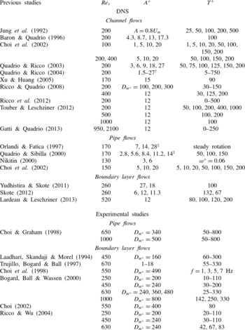
Overview of previous DNS studies on wall oscillation flow control.
 $\mathit{Re}_{{\it\tau}}$
for the pipe flow was calculated from
 $\mathit{Re}_{D}=U_{m}D/{\it\nu}$
. Here
 $\mathit{Re}_{{\it\tau}}$
for the boundary layer was calculated from
 $\mathit{Re}_{{\it\delta}}^{\ast }=U_{\infty }{\it\delta}^{\ast }/{\it\nu}$
and
 $\mathit{Re}_{{\it\theta}}=U_{\infty }{\it\theta}/{\it\nu}$
,
 $\text{}^{\dagger }A^{+}$
was calculated from the displacement,
 $D_{m^{+}}$
, and
 $\text{}^{\ddagger }A^{+}$
was calculated from the rotation number for pipe flow.

While most of previous DNS studies on wall oscillation flow control listed in table 1 have been confined to
 $\mathit{Re}_{{\it\tau}}=200$
or 400, several simulations of wall oscillation have been performed at higher Reynolds numbers. Simulations of the wall oscillation at
 $\mathit{Re}_{{\it\tau}}=400$
were performed by Choi et al. (Reference Choi, Xu and Sung2002) with
 $A^{+}=5$
, 10 and 20, and
 $T^{+}=50$
, 100, 150 and 200. A significant decrease in the drag reduction was observed as the Reynolds number increased from
 $\mathit{Re}_{{\it\tau}}=100$
and 400, and the parameters were scaled by wall units. However, the Reynolds number effect on drag reduction was not assessed directly. Instead, they presented a scaling function linking the input parameters to the level of drag reduction. They proposed a combined parameter
 $V_{c}^{+}$
, which included a Reynolds number dependence,
 $V_{c}^{+}\sim \mathit{Re}_{{\it\tau}}^{-0.2}$
. They obtained a correlation of
 ${\mathcal{D}}{\mathcal{R}}\sim aV_{c}^{+}+bV_{c}^{+2}$
, where
 $a$
and
 $b$
are constant, implying that the Reynolds number effect in this correlation is between
 $\mathit{Re}_{{\it\tau}}^{-0.2}$
and
 $\mathit{Re}_{{\it\tau}}^{-0.4}$
. The square term (
 $bV_{c}^{+2}$
) dominates except for
 $V_{c}^{+}<0.05$
, suggesting that a Reynolds number effect is close to
 $\mathit{Re}_{{\it\tau}}^{-0.4}$
.
Ricco & Quadrio (Reference Ricco and Quadrio2008) performed wall oscillation simulations at
 $\mathit{Re}_{{\it\tau}}=400$
, with
 $T^{+}=30$
, 125 and 200 and
 $A^{+}=12$
. A decrease in the drag reduction from the
 $\mathit{Re}_{{\it\tau}}=200$
case was again shown. An interesting feature of their simulations is that the change in the drag reduction, when the Reynolds number was increased from
 $\mathit{Re}_{{\it\tau}}=200$
to 400, was larger for higher values of
 $T^{+}$
. Recently, Touber & Leschziner (Reference Touber and Leschziner2012) studied wall oscillation at
 $\mathit{Re}_{{\it\tau}}=500$
and 1000. The lower drag reduction at higher Reynolds numbers was proposed to be attributed to the large-scale structures, which will become more influential over the wall as the Reynolds number increases.
No Reynolds number effect of wall oscillation has been observed in experiment. Choi & Graham (Reference Choi and Graham1998) conducted pipe flow experiments at two Reynolds numbers:
 $\mathit{Re}_{D}=2.33\times 10^{4}$
and
 $3.63\times 10^{4}$
, with the corresponding Reynolds number ratio of
 $\mathit{Re}_{2}/\mathit{Re}_{1}=1.47$
. The pipe was oscillated at a frequency of up to 50 Hz with a fixed angle of
 $30^{\circ }$
. Due to the use of a constant oscillation amplitude, the wall velocity
 $A^{+}$
varied with the oscillating period
 $T^{+}$
and also with the Reynolds number. This makes a direct comparison between the two Reynolds numbers difficult. In figure 2 of their paper,
 ${\mathcal{D}}{\mathcal{R}}$
for the higher-Reynolds-number flow appears to be consistently larger than
 ${\mathcal{D}}{\mathcal{R}}$
for the lower Reynolds number, and this was mainly because 30 % smaller
 $A^{+}$
values were used at the lower Reynolds number. When scaled to compensate for different
 $A^{+}$
values, similar
 ${\mathcal{D}}{\mathcal{R}}$
values are obtained from the two Reynolds numbers, and the difference between the two cases is much smaller than the expected difference of
 ${\rm\Delta}{\mathcal{D}}{\mathcal{R}}=7\,\%$
for
 $A^{+}=12$
. Ricco & Wu (Reference Ricco and Wu2004) studied the boundary-layer wall oscillation experimentally using three different Reynolds numbers (
 $\mathit{Re}_{{\it\theta}}=500$
, 950 and 1400). Their results did not show any clear Reynolds number effect. This is again mainly due to the experimental uncertainty associated with the wall shear stress measurement on an oscillating wall. The expected
 ${\mathcal{D}}{\mathcal{R}}$
variations for these Reynolds numbers is within the uncertainty range reported.
It is interesting to note that the Reynolds number effect is much less clear in the boundary-layer flow. As already mentioned, no Reynolds number effect was observed in the boundary-layer experiment of Ricco & Wu (Reference Ricco and Wu2004). Numerical simulations of the turbulent boundary layer with wall oscillation have been performed in a few studies (Yudhistira & Skote Reference Yudhistira and Skote2011; Skote Reference Skote2012; Lardeau & Leschziner Reference Lardeau and Leschziner2013). A drag reduction of
 ${\mathcal{D}}{\mathcal{R}}=29.4\,\%$
was obtained at
 $\mathit{Re}_{{\it\theta}}=500$
(or
 $\mathit{Re}_{{\it\tau}}=260$
) for
 $A^{+}=12$
and
 $T^{+}=132$
(Skote Reference Skote2012). DNS of turbulent boundary layer at
 $\mathit{Re}_{{\it\tau}}=520$
was conducted by Lardeau & Leschziner (Reference Lardeau and Leschziner2013) for
 $A^{+}=12$
at four different oscillation frequencies:
 $T^{+}=80$
, 100, 120 and 200, with the largest drag reduction of
 ${\mathcal{D}}{\mathcal{R}}=25\,\%$
at
 $T^{+}=80$
. In these numerical studies, a single Reynolds number was used, making a direct comparison for the Reynolds number effect between different studies less straightforward. Comparing Skote (Reference Skote2012) and Lardeau & Leschziner (Reference Lardeau and Leschziner2013) gives a change of
 ${\rm\Delta}{\mathcal{D}}{\mathcal{R}}=4.4\,\%$
between
 $\mathit{Re}_{{\it\tau}}=260$
and
 $\mathit{Re}_{{\it\tau}}=520$
, but it should be noted that different
 $T^{+}$
values were used in their simulations. Skote (Reference Skote2012) compared his boundary-layer DNS results at
 $\mathit{Re}_{{\it\theta}}=500$
with channel flow data available in literature using an equivalent
 $\mathit{Re}_{{\it\theta}}$
numbers for the channel flow. Significantly smaller drag reductions were found in the boundary layer compared with the channel flow, and this difference is too large for the Reynolds number effect alone. This apparent difference from the channel flow (DNS) results may also be due to the different flow physics between the channel and the boundary layer, and this can only be answered by further boundary layer DNS and experimental studies.
Some Reynolds number effect for travelling waves was observed. Quadrio et al. (Reference Quadrio, Ricco and Viotti2009) reported that the maximum drag reduction depended weakly on the Reynolds number; the drag reduction decreased from 48 % to 42 % as the Reynolds number increased from
 $\mathit{Re}_{{\it\tau}}=200$
to 400. Recently, Gatti & Quadrio (Reference Gatti and Quadrio2013) studied the Reynolds number effect on travelling waves using a small computational domain size of (
 $1.2h\times 2h\times 0.6h$
) to reduce the computational cost. Due to the use of a small domain size, they were able to increase the Reynolds number to
 $\mathit{Re}_{{\it\tau}}=950$
and 2100. They chose several areas in the parameter domain (
 ${\it\omega}^{+},{\it\kappa}_{x}^{+}$
), and claimed that the sensitivity to Reynolds number varied among different locations in the parameter domain, especially at the boundary of drag reduction and drag increase regions. While the impact of the small computational domain size was carefully assessed and validated at a lower Reynolds number, this type of approach can become more useful once their results are compared with full-scale DNS results or experimental data.
The effect of Reynolds number was also observed in other control methods. A decrease in the drag reduction achieved on both opposition control and suboptimal control was reported as the Reynolds number was increased (Iwamoto, Suzuki & Kasagi Reference Iwamoto, Suzuki and Kasagi2002). By damping the near-wall velocity fluctuations, Iwamoto et al. (Reference Iwamoto, Fukagata, Kasagi and Suzuki2005) suggested a much weaker Reynolds number dependence for drag reduction. This could provide a theoretical limit of drag reduction at higher Reynolds numbers, but real drag reduction achievable would be significantly lower than this limit, implying a stronger Reynolds number dependence. The effect of Reynolds number on opposition control was studied by Chang, Collis & Ramakrishnan (Reference Chang, Collis and Ramakrishnan2002). The drag reduction again deteriorated as the Reynolds number was increased. They also reported that, when scaled in wall units, the optimal location of the sensing plane moved towards the wall, indicating that the optimal control parameter could be Reynolds number dependent.
A strong Reynolds number effect was observed in Lorentz force flow control. Berger et al. (Reference Berger, Kim, Lee and Lim2000) performed a parametric study with different oscillating periods
 $T^{+}$
, force strength
 $St$
and penetration depth
 ${\rm\Delta}^{+}$
at three Reynolds numbers i.e.
 $\mathit{Re}_{{\it\tau}}=100$
, 200 and 400. They found that the maximum
 ${\mathcal{D}}{\mathcal{R}}$
for a given
 $T^{+},{\rm\Delta}^{+}$
decreased sharply when the Reynolds number increased. For example, estimated from figure 11 in their paper, at
 $T^{+}=100$
,
 ${\rm\Delta}^{+}=5$
, the maximum
 ${\mathcal{D}}{\mathcal{R}}$
is
 $42\,\%$
,
 $26\,\%$
and
 $7\,\%$
for
 $\mathit{Re}_{{\it\tau}}=100$
, 200 and 400, respectively, suggesting a
 $\mathit{Re}_{{\it\tau}}^{-1.3}$
scaling, which is much stronger than the Reynolds number effect observed in other control methods.
3. Computational details
3.1. Numerical method
Fully developed turbulent channel flow with wall control is considered using DNS. The results presented are generated by a DNS code (Chung & Talha Reference Chung and Talha2011), based on the fully implicit fractional step method proposed by Kim, Baek & Sung (Reference Kim, Baek and Sung2002), in which a Crank–Nicolson discretisation is used for both the diffusion and convective terms. The Navier–Stokes equations are solved in a Cartesian coordinate system. Using block LU decomposition each velocity equation is split into three one-dimensional problems which are solved using suitable banded matrix algorithms. The pressure is updated via the Poisson equation, taking advantage of the uniform grid discretisation in the streamwise and spanwise directions by performing a combination of a two-dimensional Fourier transform and a tridiagonal matrix inversion. Various versions of the code have been used for DNS and large eddy simulations (LES) (Chung & Talha Reference Chung and Talha2011; Jewkes, Chung & Carpenter Reference Jewkes, Chung and Carpenter2011; Jung & Chung Reference Jung and Chung2012; Chung & Hurst Reference Chung, Hurst, Zhou, Liu, Huang and Hodges2014).
When considering parallelisation using MPI, it is preferable to retain the data from the full domain length in the direction of any one-dimensional algorithms. Therefore, a pencil structure is adopted, dividing the processes into a two-dimensional grid. The code makes use of the 2DECOMP&FFT library developed by Laizet & Li (Reference Laizet and Li2011), which performs optimised transpositions when all the data is required in a particular direction. It utilises a set of halo cells for calculations requiring only local data, to reduce the number of necessary transpositions. Parallel I/O is also used to remove the dependency upon writing data and improve efficiency. Simulations were performed using the local cluster (Minerva) with 6000 Intel Xeon X5650 Westmere-EP 2.66 GHz cores at the Centre for Scientific Computing, University of Warwick. The higher-Reynolds-number simulations at
 $\mathit{Re}_{{\it\tau}}=1600$
were run on 1024 cores on HECToR and ARCHER (www.archer.ac.uk), the UK National High Performance Computing Facility.
3.2. Simulation parameters
DNS of the turbulent channel flow were performed at four Reynolds numbers
 $\mathit{Re}_{{\it\tau}}=200$
, 400, 800 and 1600, based on the frictional velocity of the no-control case,
 $u_{{\it\tau}0}$
, and the channel half-width,
 $h$
. The simulations were run with a constant mass flow rate by dynamically adjusting the pressure gradient. The length of the computational domain is chosen so that the same wall control parameters, scaled by wall units, can be studied at each of the Reynolds numbers, due to the requirement of an integer number of waves within the domain.
The domain sizes, grid sizes and resolutions used in the main simulations are shown in table 2. Throughout this paper
 $\text{}^{+}$
represents the wall units based on
 $u_{{\it\tau}0}$
. The number of grid points was adopted such that the grid spacing was fixed with
 ${\rm\Delta}x^{+}=10$
and
 ${\rm\Delta}z^{+}=5$
. A time step size of
 ${\rm\Delta}t^{+}\approx 0.12$
was used, with time averaging taken over at least
 $t^{+}=7200$
after the initial transient. All statistics were obtained using plane averaging in the streamwise and spanwise directions as well as time averaging.
Parameters of the channel flow simulations at the four Reynolds numbers studied. Here
 $L_{x},L_{y}$
and
 $L_{z}$
are the computational domain size in the
 $x,y$
and
 $z$
directions,
 $N_{x},N_{y}$
and
 $N_{z}$
are the corresponding grid sizes and
 $\mathit{Re}=U_{m}h/{\it\nu}$
is the bulk mean Reynolds number.

The current simulations are restricted to forward travelling waves, corresponding to positive values of
 ${\it\omega}$
and
 ${\it\kappa}_{x}$
. Using these parameters, the region of maximum drag reduction and the region of drag increase can be investigated. The maximum wall velocity was also fixed at
 $A^{+}=12$
to aid in comparison with previous work (Quadrio et al.
Reference Quadrio, Ricco and Viotti2009; Touber & Leschziner Reference Touber and Leschziner2012). At
 $\mathit{Re}_{{\it\tau}}=200,400$
and 800, a series of simulations were performed using all combinations of the control parameters
 ${\it\omega}^{+}$
of
 $0.01{-}0.18$
and
 ${\it\kappa}_{x}^{+}$
of
 $0.002{-}0.016$
. This gives a good view over the region of interest in the (
 ${\it\omega},{\it\kappa}_{x}$
) drag reduction map (Quadrio et al.
Reference Quadrio, Ricco and Viotti2009). For the wall oscillation and stationary wave, extra points were chosen in the region of the optimal,
 ${\it\omega}^{+}=0.06{-}0.1$
and
 ${\it\lambda}^{+}=1000{-}1250$
. The parameters which achieved the maximum drag reduction for the wall oscillation and stationary wave were also run at
 $\mathit{Re}_{{\it\tau}}=1600$
. To the best of the authors’ knowledge, this is the highest Reynolds number attempted for flow control DNS using a full domain.
3.3. Grid sensitivity study
First, the effect of the computational domain size was considered through a sensitivity study at
 $\mathit{Re}_{{\it\tau}}=200$
. Two simulations of larger computational domain sizes were performed with the same grid resolution as in the CH200 case in table 2. The computational domain size was doubled in the streamwise direction (
 $L_{x}=32h$
) and spanwise direction (
 $L_{z}=12h$
), respectively. A comparison of DNS results for the larger domain sizes (
 $32h\times 2h\times 6h$
and
 $16h\times 2h\times 12h$
) with the baseline case shows that the skin-friction coefficients were not affected by doubling the domain size. The final domain size chosen (
 $16h\times 2h\times 6h$
) is similar to that used by Bernardini et al. (Reference Bernardini, Pirozzoli and Orlandi2014) for channel flow DNS at
 $\mathit{Re}_{{\it\tau}}=4000$
.
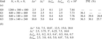
Parameters used in a grid sensitivity study. (a) Four grid resolutions tested for no-control and wall oscillation cases. Here
 $C_{f}$
values are for no-control cases at
 $\mathit{Re}_{{\it\tau}}=200$
and
 ${\mathcal{D}}{\mathcal{R}}$
values are the amount of drag reduction for the optimal wall oscillation case,
 ${\it\omega}^{+}=0.06$
at
 $\mathit{Re}_{{\it\tau}}=200,400$
and 800. (b) Various grid spacings tested from the baseline (G1) grid for a further grid sensitivity study. Here
 $\dagger$
indicates the final grid spacings chosen.

An extensive grid sensitivity study was performed at the lowest Reynolds number (
 $\mathit{Re}_{{\it\tau}}=200$
) due to the computational cost required. Table 3(a) shows samples of grids tested including two very fine grids (G0 and G1). The G0 grid uses
 $1280\times 380\times 480$
grid points with a total number of 233 million. The G1 grid is the same as the G0 grid except a larger streamwise grid spacing (
 ${\rm\Delta}x^{+}=5$
), and a total number of 117 million grid points were used. The skin-friction coefficient
 $C_{f}$
values at
 $\mathit{Re}_{{\it\tau}}=200$
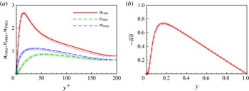
given in table 3(a) are very similar for all cases, and the difference is approximately 1 %. DNS results of flow quantities show little difference between the G0 and G1 grids, so the G1 grid was used as the baseline grid for a further grid sensitivity study. The root-mean-squared (r.m.s.) velocity (
 $u_{i,rms}^{+}$
) fluctuations and the Reynolds shear stress (
 $-\overline{uv}$
) from the G1 grid are shown in figure 1. Also included in the figure are the DNS data of Kim, Moin & Moser (Reference Kim, Moin and Moser1987) at
 $\mathit{Re}_{{\it\tau}}=180$
. The present DNS results for no-control case exhibit an excellent agreement with the available DNS data.
Present DNS data for no-control case on the baseline (G1) grid at
 $\mathit{Re}_{{\it\tau}}=200$
. (a) Velocity fluctuation,
 $u_{i,rms}^{+}$
, and (b) Reynolds shear stress,
 $-\overline{uv}$
. Symbols are DNS data of Kim et al. (Reference Kim, Moin and Moser1987) at
 $\mathit{Re}_{{\it\tau}}=180$
.

The grid resolution was systematically changed only in one direction at a time while grid resolutions in the other two directions remain unchanged from the baseline (G1) grid;
 ${\rm\Delta}y_{\mathit{min}}^{+}$
and
 ${\rm\Delta}y_{\mathit{max}}^{+}$
were also changed separately. The grid spacings tested are shown in table 3(b). Various flow properties including the skin-friction coefficient
 $C_{f}$
were compared with the values from the baseline grid case. From this grid sensitivity study, the G3 grid was chosen based on the accuracy and also computational resources required to create a drag reduction map.
The grid sensitivity study was then extended to higher Reynolds numbers (
 $\mathit{Re}_{{\it\tau}}=400$
and 800). The accuracy of the G3 grid has been thoroughly assessed. First, the relation between
 $Re$
and
 $\mathit{Re}_{{\it\tau}}$
is compared with other DNS studies (Moser, Kim & Mansour Reference Moser, Kim and Mansour1999; Iwamoto et al.
Reference Iwamoto, Suzuki and Kasagi2002; Tanahashi et al.
Reference Tanahashi, Kang, Miyamoto, Shiokawa and Miyauchi2004; del Álamo & Jiménez Reference del Álamo and Jiménez2003; del Álamo et al.
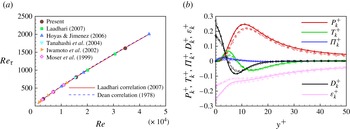
Reference del Álamo, Jiménez, Zandonade and Moser2004; Hoyas & Jiménez Reference Hoyas and Jiménez2006) in figure 2(a) to examine whether
 $C_{f}$
is correctly predicted in the present DNS. Also included in figure 2(a) are two correlations proposed by Dean (Reference Dean1978) based on experiments and by Laadhari (Reference Laadhari2007) based on DNS data.
 $U_{m}^{+}\ (=\sqrt{2/C_{f}})$
values are also compared well with other DNS data (not shown here). The kinetic energy budget terms for all four Reynolds numbers are compared with the DNS data from literature at similar Reynolds numbers (Kim et al.
Reference Kim, Moin and Moser1987; Moser et al.
Reference Moser, Kim and Mansour1999; del Álamo et al.
Reference del Álamo, Jiménez, Zandonade and Moser2004; Hoyas & Jiménez Reference Hoyas and Jiménez2006). The
 $\mathit{Re}_{{\it\tau}}=200$
and 1600 cases are displayed in figure 2(b). Figure 2 clearly shows that the present DNS results on the final grid are in good agreement with other DNS studies and also with the correlations proposed by Dean (Reference Dean1978) and Laadhari (Reference Laadhari2007).
Present DNS data for no-control case on the final (G3) grid at four Reynolds numbers considered: (a)
 $\mathit{Re}_{{\it\tau}}$
versus
 $Re$
; (b) turbulence kinetic energy budget terms. Dashed lines are the present DNS data at
 $\mathit{Re}_{{\it\tau}}=200$
and solid lines are the present DNS data at
 $\mathit{Re}_{{\it\tau}}=1600$
. Symbols are DNS data of Kim et al. (Reference Kim, Moin and Moser1987) for
 $\mathit{Re}_{{\it\tau}}=180$
(○) and Hoyas & Jiménez (Reference Hoyas and Jiménez2006) for
 $\mathit{Re}_{{\it\tau}}=2000$
(♢).

In addition to the no-control case, wall oscillation simulations for the optimal case of
 ${\it\omega}^{+}=0.06$
were performed at three Reynolds numbers to ascertain the effect of grid resolution on flow control results. Based on the
 $\mathit{Re}_{{\it\tau}}=200$
results described earlier, only the G2 and G3 grids were considered at high Reynolds numbers as it was found that DNS results are more sensitive to the resolution in the streamwise direction. The difference in
 ${\mathcal{D}}{\mathcal{R}}$
prediction between the two grids are shown in table 3(a) at
 $\mathit{Re}_{{\it\tau}}=200$
, 400 and 800. The effect on
 ${\mathcal{D}}{\mathcal{R}}$
prediction is found to be smaller than
 ${\rm\Delta}{\mathcal{D}}{\mathcal{R}}=1\,\%$
. A similar trend was observed for the stationary wave case.
4. Results and discussion
4.1. Drag reduction map
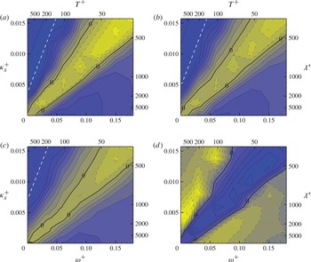
Figure 3 shows contours of the drag reduction values achieved at three Reynolds numbers,
 $\mathit{Re}_{{\it\tau}}=200,400$
and 800, with using 86, 90 and 106 simulations, respectively. The drag reduction map at
 $\mathit{Re}_{{\it\tau}}=200$
is very similar to that shown in Quadrio et al. (Reference Quadrio, Ricco and Viotti2009). Please note that only forward travelling waves (
 $c>0$
) were considered in this study as this half of the parameter domain contains the optimal travelling wave case while Quadrio et al. (Reference Quadrio, Ricco and Viotti2009) considered both forward and backward travelling waves. In this study, the amount of drag reduction can be defined as
 ${\mathcal{D}}{\mathcal{R}}=\left(1-(C_{f}/C_{f,0})\right)\times 100\,(\%)$
, where
 $C_{f,0}$
is the skin-friction coefficient for the no-control case. The maximum drag reduction at
 $\mathit{Re}_{{\it\tau}}=200$
is approximately
 ${\mathcal{D}}{\mathcal{R}}_{\mathit{max}}=50$
, and the optimal control parameters are
 ${\it\omega}^{+}=0.02$
(
 $T^{+}=300$
) and
 ${\it\kappa}_{x}^{+}=0.008$
(
 ${\it\lambda}^{+}=800$
). It is interesting to note that at first glance, drag reduction maps at the higher Reynolds numbers (
 $\mathit{Re}_{{\it\tau}}=400$
and 800) appear to be similar to that at
 $\mathit{Re}_{{\it\tau}}=200$
, indicating that the overall drag reduction and drag increase characteristics of the travelling wave are not affected significantly by increasing the Reynolds number: the large
 ${\mathcal{D}}{\mathcal{R}}$
values are observed in the
 ${\mathcal{D}}{\mathcal{R}}$
peak region around
 $c_{\mathit{DR}}^{+}\approx 4$
while a drag increase is observed in a narrow region around
 $c_{\mathit{DI}}^{+}\approx 10$
at all three Reynolds numbers. A line of the minimum
 $\boldsymbol{{\rm\nabla}}{\mathcal{D}}{\mathcal{R}}$
passing through the
 ${\mathcal{D}}{\mathcal{R}}_{\mathit{max}}$
location is displayed in the
 ${\mathcal{D}}{\mathcal{R}}$
map to indicate the location for the
 ${\mathcal{D}}{\mathcal{R}}$
peak region:
 $$\begin{eqnarray}{\it\kappa}_{x}^{+}={\it\omega}^{+}/c_{\mathit{DR}}^{+}+{\it\kappa}_{x,s}^{+}.\end{eqnarray}$$
Please note
 ${\it\kappa}_{x,s}^{+}$
is where the above line intersects the
 ${\it\omega}^{+}=0$
axis in the
 ${\mathcal{D}}{\mathcal{R}}$
map.
Drag reduction map (
 ${\it\omega}^{+}$
,
 ${\it\kappa}_{x}^{+}$
) for the forward travelling waves at (a)
 $\mathit{Re}_{{\it\tau}}=200$
, (b)
 $\mathit{Re}_{{\it\tau}}=400$
and (c)
 $\mathit{Re}_{{\it\tau}}=800$
. Contour levels are drawn at 5 % intervals. The dark (blue online) indicates a drag reduction and the bright (yellow online) colour indicates a drag increase. White dashed lines indicate the location for the local
 ${\mathcal{D}}{\mathcal{R}}$
maxima. (d) For
 ${\rm\Delta}{\mathcal{D}}{\mathcal{R}}={\mathcal{D}}{\mathcal{R}}_{800}-{\mathcal{D}}{\mathcal{R}}_{200}$
, change in drag reduction from
 $\mathit{Re}_{{\it\tau}}=200$
to 800. The bright (yellow online) colour indicates a negative
 ${\rm\Delta}{\mathcal{D}}{\mathcal{R}}$
, and the dark (blue online) indicates a positive
 ${\rm\Delta}{\mathcal{D}}{\mathcal{R}}$
.

While the overall similarity of the drag reduction map is evident at different Reynolds numbers, figure 3 shows that the absolute value of drag change (both drag reduction and drag increase) is decreased when the Reynolds number is increased. The maximum drag reduction at
 $\mathit{Re}_{{\it\tau}}=400$
is reduced to
 ${\mathcal{D}}{\mathcal{R}}_{\mathit{max}}=44$
with the optimal control parameters changed slightly. At the optimal control parameters, the difference in the maximum
 ${\mathcal{D}}{\mathcal{R}}$
achieved at these two Reynolds numbers is quite significant,
 ${\rm\Delta}{\mathcal{D}}{\mathcal{R}}=-6$
, which means by doubling the Reynolds number from
 $\mathit{Re}_{{\it\tau}}=200$
, drag reduction has already become roughly 10 % less effective than the lower-Reynolds-number case. The maximum
 ${\mathcal{D}}{\mathcal{R}}$
decreases further to
 ${\mathcal{D}}{\mathcal{R}}_{\mathit{max}}=40$
at
 $\mathit{Re}_{{\it\tau}}=800$
. It is worthwhile to note that the optimal control parameters for
 $\mathit{Re}_{{\it\tau}}=800$
changes slightly from the lower-Reynolds-number values, and this will be addressed later. The peak region for large
 ${\mathcal{D}}{\mathcal{R}}$
values also appears to move towards a smaller
 ${\it\omega}^{+}$
and larger
 ${\it\kappa}_{x}^{+}$
region. It is observed that the region of the parameter space in which the drag increase is found diminishes as the Reynolds number is increased. There is a valley region in the drag reduction map along
 $c_{\mathit{DI}}^{+}\approx 10$
where
 ${\mathcal{D}}{\mathcal{R}}$
is negative. This valley still exists at higher Reynolds numbers, but drag increase in the valley region becomes less pronounced at higher Reynolds numbers, making the valley shallow. Gatti & Quadrio (Reference Gatti and Quadrio2013) suggested that this valley region widens as the Reynolds number increases. Because our primary interest is in the drag reduction region, however, it is not quite clear from the present study whether this valley region widens or not as the Reynolds number increases.
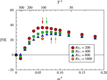
Drag reduction for the wall oscillation case,
 ${\it\kappa}_{x}^{+}=0$
. The vertical arrow indicates the location for the maximum
 ${\mathcal{D}}{\mathcal{R}}$
at each Reynolds number.

Figure 3(d) shows the change in drag reduction values,
 ${\rm\Delta}{\mathcal{D}}{\mathcal{R}}={\mathcal{D}}{\mathcal{R}}_{800}-{\mathcal{D}}{\mathcal{R}}_{200}$
, to illustrate the effect of increasing the Reynolds number from
 $\mathit{Re}_{{\it\tau}}=200$
to 800 on
 ${\mathcal{D}}{\mathcal{R}}$
. With control parameters close to that of the maximum drag reduction, (
 ${\it\omega}_{\mathit{opt}}^{+}$
,
 ${\it\kappa}_{x,\mathit{opt}}^{+}$
), the change is large and negative with a reduction of up to
 ${\rm\Delta}{\mathcal{D}}{\mathcal{R}}=-12$
. In the valley region of the drag reduction map, the magnitude of the drag increase also becomes smaller at higher Reynolds numbers corresponding to positive values of
 ${\rm\Delta}{\mathcal{D}}{\mathcal{R}}$
. For example, in the middle of the drag increase valley (
 ${\it\omega}^{+}=0.09$
and
 ${\it\kappa}_{x}^{+}=0.008$
), drag increases are
 ${\mathcal{D}}{\mathcal{R}}=-17$
,
 $-10$
and
 $-5$
at
 $\mathit{Re}_{{\it\tau}}=200$
, 400 and 800, respectively, resulting in a difference in
 ${\mathcal{D}}{\mathcal{R}}$
between
 $\mathit{Re}_{{\it\tau}}=200$
and 800 of
 ${\rm\Delta}{\mathcal{D}}{\mathcal{R}}=12$
.
4.2. Reynolds number effect
The drag reduction results for the wall oscillation (
 ${\it\kappa}_{x}^{+}=0$
) for all the Reynolds numbers are presented in figure 4. The present results shown in figure 4 clearly displays the decrease in the value of
 ${\mathcal{D}}{\mathcal{R}}$
as the Reynolds number is increased. At all three Reynolds numbers,
 ${\mathcal{D}}{\mathcal{R}}$
increases initially with
 ${\it\omega}^{+}$
to attain a maximum
 ${\mathcal{D}}{\mathcal{R}}$
at
 ${\it\omega}_{\mathit{opt}}^{+}$
, and then decreases gradually. One interesting feature of the wall oscillation is that the optimal frequency increases slightly from
 ${\it\omega}_{\mathit{opt}}^{+}=0.06$
(
 $T^{+}=100$
) at
 $\mathit{Re}_{{\it\tau}}=200$
to
 ${\it\omega}_{\mathit{opt}}^{+}=0.07$
at
 $\mathit{Re}_{{\it\tau}}=400$
, and
 ${\it\omega}_{\mathit{opt}}^{+}=0.08$
at
 $\mathit{Re}_{{\it\tau}}=800$
although the
 ${\mathcal{D}}{\mathcal{R}}$
peak becomes broader as the Reynolds number increases, and the
 ${\mathcal{D}}{\mathcal{R}}_{\mathit{max}}$
is not easily discernible. The drag reduction at
 ${\it\omega}^{+}=0.06$
(
 $T^{+}=100$
) is calculated up to
 $\mathit{Re}_{{\it\tau}}=1600$
. At this Reynolds number, the drag reduction has been reduced from
 ${\mathcal{D}}{\mathcal{R}}=37$
to
 ${\mathcal{D}}{\mathcal{R}}=22$
, corresponding to a
 ${\rm\Delta}{\mathcal{D}}{\mathcal{R}}=-15$
decrease from the
 $\mathit{Re}_{{\it\tau}}=200$
case, which means a 40 % less effectiveness from the low-Reynolds-number result. While the change in
 ${\mathcal{D}}{\mathcal{R}}$
at the optimal value,
 ${\it\omega}_{\mathit{opt}}^{+}$
, is greater, there appears to be less of an effect of Reynolds number at larger values of
 ${\it\omega}^{+}$
(corresponding to smaller
 $T^{+}$
) in the drag reduction region. Ricco & Quadrio (Reference Ricco and Quadrio2008) reported a similar trend using results from
 $\mathit{Re}_{{\it\tau}}=400$
.
Wall oscillation
 ${\mathcal{D}}{\mathcal{R}}$
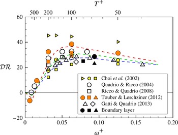
data reported in literature have been examined to identify the Reynolds number dependence. Figure 5 shows
 ${\mathcal{D}}{\mathcal{R}}$
data of Choi et al. (Reference Choi, Xu and Sung2002), Quadrio & Ricco (Reference Quadrio and Ricco2004), Ricco & Quadrio (Reference Ricco and Quadrio2008), Touber & Leschziner (Reference Touber and Leschziner2012) and Gatti & Quadrio (Reference Gatti and Quadrio2013). Some Reynolds number effect is discernible in the data, but there is considerable of scatter between different studies. This is partly because different amplitudes and oscillation frequencies have been used in various studies as summarised in table 1. A clear decrease in
 ${\mathcal{D}}{\mathcal{R}}$
is shown in Choi et al. (Reference Choi, Xu and Sung2002) (yellow symbols), but their
 ${\mathcal{D}}{\mathcal{R}}$
values are somewhat smaller than the
 ${\mathcal{D}}{\mathcal{R}}$
values reported in other studies at the same Reynolds numbers. Quadrio & Ricco (Reference Quadrio and Ricco2004) and Ricco & Quadrio (Reference Ricco and Quadrio2008) (open symbols) display similar trend at
 $\mathit{Re}_{{\it\tau}}=200$
and 400. A similar trend is also seen in Touber & Leschziner (Reference Touber and Leschziner2012) (orange symbols) at
 $\mathit{Re}_{{\it\tau}}=200$
, 500 and 1000. Also included are the DNS data of Gatti & Quadrio (Reference Gatti and Quadrio2013) (open symbols) at
 $\mathit{Re}_{{\it\tau}}=950$
and 2100.
The
 ${\mathcal{D}}{\mathcal{R}}$
data for the wall oscillation case,
 ${\it\kappa}_{x}^{+}=0$
, in literature: Choi et al. (Reference Choi, Xu and Sung2002), small grey (yellow) colour symbols; Quadrio & Ricco (Reference Quadrio and Ricco2004), Ricco & Quadrio (Reference Ricco and Quadrio2008) and Gatti & Quadrio (Reference Gatti and Quadrio2013), open symbols; Touber & Leschziner (Reference Touber and Leschziner2012), grey (orange) colour symbols; boundary layer (Yudhistira & Skote Reference Yudhistira and Skote2011; Skote Reference Skote2012; Lardeau & Leschziner Reference Lardeau and Leschziner2013), black symbols. Present results are shown in dashed lines. The wall oscillation amplitude is
 $A^{+}=12$
for all cases except for Choi et al. (Reference Choi, Xu and Sung2002), where the data is for
 $A^{+}=10$
.

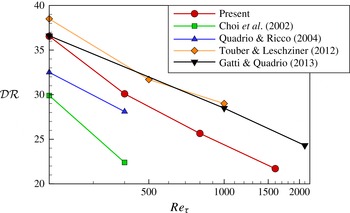
The
 ${\mathcal{D}}{\mathcal{R}}$
values for near-optimal wall oscillation cases are displayed in figure 6. The oscillation frequency used is
 ${\it\omega}^{+}=0.06$
(or
 $T^{+}=100$
) in most studies while different
 $T^{+}$
values were used in some studies:
 $T^{+}=125$
is used in Ricco & Quadrio (Reference Ricco and Quadrio2008) and
 $T^{+}=90$
in Gatti & Quadrio (Reference Gatti and Quadrio2013). All
 ${\mathcal{D}}{\mathcal{R}}$
data show a clear trend of drag reduction becoming less successful as the Reynolds number increases. The first thing to notice is that there is a large variation in the
 ${\mathcal{D}}{\mathcal{R}}$
values at
 $\mathit{Re}_{{\it\tau}}=200$
. The
 ${\mathcal{D}}{\mathcal{R}}$
values in Choi et al. (Reference Choi, Xu and Sung2002) are particularly low, and this may be partly due to a smaller oscillation amplitude (
 $A^{+}=10$
) used in their simulations. Also the decrease between
 $\mathit{Re}_{{\it\tau}}=200$
and 400 appears to be larger than in other studies, indicating a strong Reynolds number effect. The
 ${\mathcal{D}}{\mathcal{R}}$
data of Gatti & Quadrio (Reference Gatti and Quadrio2013) using a small computational domain are also included. Their
 ${\mathcal{D}}{\mathcal{R}}$
values appear to be significantly larger than the present results even though their
 ${\mathcal{D}}{\mathcal{R}}$
value for
 $\mathit{Re}_{{\it\tau}}=200$
is very similar to the
 ${\mathcal{D}}{\mathcal{R}}$
value from the present study.
Drag reduction for the near-optimal wall oscillation cases. The oscillation frequency is
 ${\it\omega}^{+}=0.06$
(
 $T^{+}=100$
), and
 $A^{+}=12$
. Please note that
 $T^{+}=125$
is used in Ricco & Quadrio (Reference Ricco and Quadrio2008) and
 $T^{+}=90$
in Gatti & Quadrio (Reference Gatti and Quadrio2013). Choi et al. (Reference Choi, Xu and Sung2002) used
 $A^{+}=10$
.

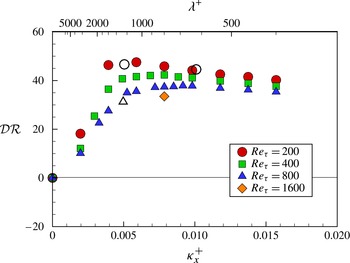
Drag reduction for the stationary wave case,
 ${\it\omega}^{+}=0$
. Open symbols are for Quadrio et al. (Reference Quadrio, Ricco and Viotti2009) (○) and Gatti & Quadrio (Reference Gatti and Quadrio2013) (▵).

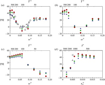
Drag reduction for the travelling wave cases. Horizontal lines through the map with (a)
 ${\it\kappa}_{x}^{+}=0.006$
, (b)
 ${\it\kappa}_{x}^{+}=0.008$
, (c)
 ${\it\kappa}_{x}^{+}=0.016$
and (d) a vertical line through the map with
 ${\it\omega}^{+}=0.02$
. Open symbols in (a) are for Quadrio et al. (Reference Quadrio, Ricco and Viotti2009) (○ for
 $\mathit{Re}_{{\it\tau}}=200$
) and Gatti & Quadrio (Reference Gatti and Quadrio2013) (▵ for
 $\mathit{Re}_{{\it\tau}}=950$
and ♢ for
 $\mathit{Re}_{{\it\tau}}=2100$
) at
 ${\it\kappa}_{x}^{+}=0.005$
, and open symbols in (d) are for Quadrio et al. (Reference Quadrio, Ricco and Viotti2009) and Gatti & Quadrio (Reference Gatti and Quadrio2013) at
 ${\it\omega}^{+}=0.012$
.

The results from the stationary wave case (
 ${\it\omega}^{+}=0$
) are presented in figure 7. Also included are the DNS data of Gatti & Quadrio (Reference Gatti and Quadrio2013). The
 ${\mathcal{D}}{\mathcal{R}}$
increases initially with
 ${\it\kappa}_{x}^{+}$
at all Reynolds numbers considered, and the rate of increase is attenuated at high Reynolds numbers. For
 ${\it\kappa}_{x}^{+}>{\it\kappa}_{x,\mathit{opt}}^{+}$
,
 ${\mathcal{D}}{\mathcal{R}}$
decreases very gradually, resulting in a broad maximum
 ${\mathcal{D}}{\mathcal{R}}$
peak at higher Reynolds numbers. It is interesting to note that like the wall oscillation case shown in figure 4, the optimal parameter for the stationary wave also appears to increase with the Reynolds number from
 ${\it\kappa}_{x,\mathit{opt}}^{+}=0.006$
(
 ${\it\lambda}^{+}=1070$
) at
 $\mathit{Re}_{{\it\tau}}=200$
although the optimal
 ${\it\kappa}_{x,\mathit{opt}}^{+}$
peak is very broad at
 $\mathit{Re}_{{\it\tau}}=800$
. Again, the change in
 ${\mathcal{D}}{\mathcal{R}}$
is significant near the optimal parameter. At
 ${\it\kappa}_{x,\mathit{opt}}^{+}=0.006$
, the drag reduction decreases from
 ${\mathcal{D}}{\mathcal{R}}=48$
at
 $\mathit{Re}_{{\it\tau}}=200$
to
 ${\mathcal{D}}{\mathcal{R}}=36$
at
 $\mathit{Re}_{{\it\tau}}=800$
, corresponding to
 ${\rm\Delta}{\mathcal{D}}{\mathcal{R}}=-12$
. However, if the wavenumber
 ${\it\kappa}_{x}^{+}=0.008$
(
 ${\it\lambda}^{+}=800$
) is considered, a drag reduction of
 ${\mathcal{D}}{\mathcal{R}}=37$
can still be achieved at
 $\mathit{Re}_{{\it\tau}}=800$
, and even a little higher at
 ${\it\kappa}_{x}^{+}=0.009$
(
 ${\it\lambda}^{+}=700$
). This means that choosing the optimal parameters determined from a low-Reynolds-number case, and scaling the parameters in wall units will not guarantee the optimal drag reduction at the higher Reynolds number. At
 $\mathit{Re}_{{\it\tau}}=1600$
, the drag is decreased further to
 ${\mathcal{D}}{\mathcal{R}}=33$
for
 ${\it\kappa}_{x}^{+}=0.008$
(
 ${\it\lambda}^{+}=800$
), making it
 ${\rm\Delta}{\mathcal{D}}{\mathcal{R}}=-15$
from the
 $\mathit{Re}_{{\it\tau}}=200$
case.
Figure 8 shows the drag reduction for the travelling wave case at Reynolds numbers up to
 $\mathit{Re}_{{\it\tau}}=800$
. Gatti & Quadrio (Reference Gatti and Quadrio2013) data (open symbols) at similar
 ${\it\omega}^{+}$
and
 ${\it\kappa}_{x}^{+}$
are also included for comparison. Looking at horizontal lines through the parameter space with
 ${\it\kappa}_{x}^{+}=0.006$
(
 ${\it\lambda}^{+}=1070$
), 0.008 (
 ${\it\lambda}^{+}=800$
) and 0.016 (
 ${\it\lambda}^{+}=400$
),
 ${\mathcal{D}}{\mathcal{R}}$
values are shown in figure 8(a–c). The Reynolds number effect is clearly seen in all
 ${\it\lambda}^{+}$
figures. Please note that Gatti & Quadrio (Reference Gatti and Quadrio2013) data included in figure 8(a) are at
 ${\it\kappa}_{x}^{+}=0.005$
. As shown from the
 ${\mathcal{D}}{\mathcal{R}}$
map in figure 3, the peak region for large
 ${\mathcal{D}}{\mathcal{R}}$
values intersects the
 ${\it\omega}^{+}=0$
axis at
 ${\it\kappa}_{x}^{+}={\it\kappa}_{x,s}^{+}$
. For small
 ${\it\kappa}_{x}^{+}$
values (
 ${\it\kappa}_{x}^{+}<{\it\kappa}_{x,s}^{+}$
), the stationary wave (
 ${\it\omega}^{+}=0$
) produces the largest
 ${\mathcal{D}}{\mathcal{R}}$
among all
 ${\it\omega}^{+}$
cases while for
 ${\it\kappa}_{x}^{+}>{\it\kappa}_{x,s}^{+}$
, the maximum
 ${\mathcal{D}}{\mathcal{R}}$
is obtained at
 ${\it\omega}^{+}=c_{\mathit{DR}}^{+}({\it\kappa}_{x}^{+}-{\it\kappa}_{x,s}^{+})$
. For instance, at
 $\mathit{Re}_{{\it\tau}}=200$
, the stationary wave is most effective for
 ${\it\kappa}_{x}^{+}\leqslant 0.004$
. As shown in figure 8(a), the
 ${\it\kappa}_{x,s}^{+}$
value also increases when the Reynolds number increases. At
 $\mathit{Re}_{{\it\tau}}=800$
, the stationary wave (
 ${\it\omega}^{+}=0$
) has the largest
 ${\mathcal{D}}{\mathcal{R}}$
for
 ${\it\kappa}_{x}^{+}\leqslant 0.006$
.
In figure 8(b), the optimal frequency is found at
 ${\it\omega}^{+}=0.02$
(
 $T^{+}=300$
) with
 $\mathit{Re}_{{\it\tau}}=200$
, giving a maximum drag reduction of
 ${\mathcal{D}}{\mathcal{R}}_{\mathit{max}}=50$
, slightly higher than that of the stationary wave, and this is consistent with Quadrio et al. (Reference Quadrio, Ricco and Viotti2009). At
 $\mathit{Re}_{{\it\tau}}=800$
, this reduces to
 ${\mathcal{D}}{\mathcal{R}}=37$
with the same frequency parameter and the
 ${\mathcal{D}}{\mathcal{R}}$
peak becomes less discernible. Figure 8(a,b) suggest that for the travelling wave, the peak region for large
 ${\mathcal{D}}{\mathcal{R}}$
moves towards higher
 ${\it\kappa}_{x}^{+}$
values as
 $\mathit{Re}_{{\it\tau}}$
increases. It is clear in figure 8(c) that the location for maximum
 $DR$
at
 ${\it\kappa}_{x}^{+}=0.016$
moves to a lower
 ${\it\omega}^{+}$
, again indicating that the peak region for large
 ${\mathcal{D}}{\mathcal{R}}$
moves with the Reynolds number. This is highlighted in the
 ${\mathcal{D}}{\mathcal{R}}$
map in figure 3 with white dashed lines.
With fixed
 ${\it\omega}^{+}=0.02$
(
 $T^{+}=300$
) in figure 8(d), the optimal location also changes from
 ${\it\kappa}_{x}^{+}=0.008$
(
 ${\it\lambda}^{+}=800$
) at
 $\mathit{Re}_{{\it\tau}}=200$
to
 ${\it\kappa}_{x}^{+}=0.01$
(
 ${\it\lambda}^{+}=640$
) at
 $\mathit{Re}_{{\it\tau}}=800$
, but again the maximum peak becomes very broad. Comparing
 ${\it\kappa}_{x}^{+}=0.008$
and
 ${\it\kappa}_{x}^{+}=0.016$
(
 ${\it\lambda}^{+}=400$
) at
 $\mathit{Re}_{{\it\tau}}=200$
, drag reduction at
 ${\it\kappa}_{x}^{+}=0.008$
is much more efficient while
 ${\mathcal{D}}{\mathcal{R}}=43$
for
 ${\it\kappa}_{x}^{+}=0.016$
, and there is a difference in the measured
 ${\mathcal{D}}{\mathcal{R}}$
levels of 7 between the two wavenumbers. At
 $\mathit{Re}_{{\it\tau}}=800$
, however, these two points achieve a similar drag reduction at
 ${\mathcal{D}}{\mathcal{R}}\approx 37$
, showing the larger reduction in
 ${\mathcal{D}}{\mathcal{R}}$
at the smaller
 ${\it\kappa}_{x}^{+}$
. At the new optimal parameter of
 ${\it\kappa}_{x}^{+}=0.01$
,
 ${\mathcal{D}}{\mathcal{R}}=40$
is obtained at
 $\mathit{Re}_{{\it\tau}}=800$
.
4.3. Reynolds number scaling
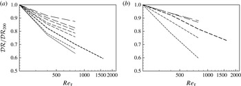
To explore the Reynolds number effect, the values of the drag reduction at the four Reynolds numbers studied are normalised by the drag reduction achieved in the
 $\mathit{Re}_{{\it\tau}}=200$
case and plotted against the Reynolds number in figure 9. Here
 ${\mathcal{D}}{\mathcal{R}}/{\mathcal{D}}{\mathcal{R}}_{200}<1$
means that drag reduction becomes less effective as the Reynolds increases from
 $\mathit{Re}_{{\it\tau}}=200$
. The results from the wall oscillation are shown in figure 9(a). It clearly shows that drag reduction for the wall oscillation deteriorates at higher Reynolds numbers, but there is a large variation in the rate of decrease in
 ${\mathcal{D}}{\mathcal{R}}/{\mathcal{D}}{\mathcal{R}}_{200}$
among the wall oscillation cases depending on
 ${\it\omega}^{+}$
values. The thick line leading to the
 $\mathit{Re}_{{\it\tau}}=1600$
represents the optimal case (
 ${\it\omega}_{\mathit{opt}}^{+}=0.06$
), indicating the drag reduction becomes much less successful at
 $\mathit{Re}_{{\it\tau}}=1600$
. The results from the stationary wave simulations are shown in figure 9(b). Again, a decrease in
 ${\mathcal{D}}{\mathcal{R}}/{\mathcal{D}}{\mathcal{R}}_{200}$
is clearly seen as the Reynolds number increases. The rate of decrease in
 ${\mathcal{D}}{\mathcal{R}}/{\mathcal{D}}{\mathcal{R}}_{200}$
varies among the cases, and the optimal case (
 ${\it\kappa}_{x,\mathit{opt}}^{+}=0.008$
) shows a better trend than the optimal wall oscillation case. It appears that the wall oscillation suffers more from the Reynolds number effect than the stationary wave. At
 $\mathit{Re}_{{\it\tau}}=1600$
, the wall oscillation becomes 40 % less effective than the
 $\mathit{Re}_{{\it\tau}}=200$
case while for the stationary wave, this is less than 30 %. Figure 9 highlights the difference in Reynolds number effect dependent on the control parameters chosen. The Reynolds number dependence is not necessarily limited to the range shown in this figure as this only shows the cases studied. It is possible that the Reynolds number dependence has larger variation than presented.
Change in drag reduction with
 $\mathit{Re}_{{\it\tau}}$
scaled by the results from the
 $\mathit{Re}_{{\it\tau}}=200$
case,
 ${\mathcal{D}}{\mathcal{R}}/{\mathcal{D}}{\mathcal{R}}_{200}$
. (a) Wall oscillation and (b) stationary wave. A longer dash length corresponds to a larger control parameter;
 ${\it\omega}^{+}$
for the wall oscillation and
 ${\it\kappa}_{x}^{+}$
for the stationary wave.

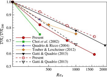
The
 ${\mathcal{D}}{\mathcal{R}}/{\mathcal{D}}{\mathcal{R}}_{200}$
values for near-optimal cases are displayed in figure 10. Wall oscillation data (Choi et al.
Reference Choi, Xu and Sung2002; Quadrio & Ricco Reference Quadrio and Ricco2004; Ricco & Quadrio Reference Ricco and Quadrio2008; Touber & Leschziner Reference Touber and Leschziner2012; Gatti & Quadrio Reference Gatti and Quadrio2013) from figure 6 are included. Also included are the stationary wave data of Gatti & Quadrio (Reference Gatti and Quadrio2013). The Reynolds number effect is clearly seen for all cases in figure 10, with large variations between the data. While Choi et al. (Reference Choi, Xu and Sung2002) display a rapid decrease in
 ${\mathcal{D}}{\mathcal{R}}$
, Gatti & Quadrio (Reference Gatti and Quadrio2013) suggest rather a moderate decrease in
 ${\mathcal{D}}{\mathcal{R}}$
for the wall oscillation. It is interesting to note that the present results indicate the Reynolds number effect is much stronger in the wall oscillation than the stationary wave, while the opposite trend was observed in Gatti & Quadrio (Reference Gatti and Quadrio2013) although they considered the
 ${\it\kappa}_{x}^{+}=0.005$
case.
Change in drag reduction,
 ${\mathcal{D}}{\mathcal{R}}/{\mathcal{D}}{\mathcal{R}}_{200}$
, for the wall oscillation case at
 ${\it\omega}^{+}=0.06$
. Open symbols indicate the optimal stationary wave cases. Present data are for
 ${\it\kappa}_{x}^{+}=0.008$
, and Gatti & Quadrio (Reference Gatti and Quadrio2013) are for
 ${\it\kappa}_{x}^{+}=0.005$
. Flow conditions for the wall oscillation are given in figure 6.

In this study, a scaling in the form
 $\mathit{Re}_{{\it\tau}}^{-{\it\alpha}}$
is calculated from
 ${\mathcal{D}}{\mathcal{R}}/{\mathcal{D}}{\mathcal{R}}_{200}$
to quantify the effect of the Reynolds number. A large (positive) value of
 ${\it\alpha}$
corresponds to a large decrease in
 ${\mathcal{D}}{\mathcal{R}}$
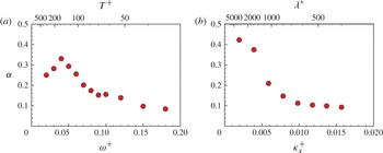
as the Reynolds number increases, and can therefore be interpreted as an unfavourable scaling. The calculated scalings for the wall oscillation and stationary wave control are shown in figure 11 and also summarised in table 4. For the wall oscillation, large values of
 ${\it\alpha}$
are obtained at lower values of
 ${\it\omega}^{+}$
with the largest
 ${\it\alpha}$
at
 ${\it\omega}^{+}=0.04$
(
 $T^{+}=150$
), emphasising the fact that the drag reduction is severely affected by the Reynolds number effect. The
 ${\it\alpha}$
value is still quite large near
 ${\it\omega}^{+}=0.06$
(
 $T^{+}=100$
), the optimal value for
 $\mathit{Re}_{{\it\tau}}=200$
. Ricco & Quadrio (Reference Ricco and Quadrio2008) also suggested that a stronger effect of Reynolds number occurs for smaller
 ${\it\omega}^{+}$
(large
 $T^{+}$
). The scaling is improved for
 ${\it\omega}^{+}>0.06$
, partly as the optimal value of
 ${\it\omega}^{+}$
is increasing with the Reynolds number; at
 ${\it\omega}^{+}=0.08$
(
 $T^{+}=75$
), the optimal value for
 $\mathit{Re}_{{\it\tau}}=800$
, the scaling value is
 ${\it\alpha}\approx 0.17$
. The scaling is further improved at larger
 ${\it\omega}^{+}$
with
 ${\it\alpha}\approx 0.1$
. There is no universal
 ${\it\alpha}$
value which can be applied for a wide range of control parameters. Instead, a large variation in
 ${\it\alpha}$
values is obtained. The present DNS results demonstrate that this type of scaling does not represent the Reynolds number dependence observed in the spanwise wall forcing flow control. It is interesting to note that Choi et al. (Reference Choi, Xu and Sung2002) used
 ${\it\alpha}=0.4$
to scale their wall oscillation
 $S^{+}$
parameter.
Reynolds number scaling parameter
 ${\it\alpha}$
for (a) wall oscillation and (b) stationary wave.

The
 ${\mathcal{D}}{\mathcal{R}}$
scalings for (a) wall oscillation and (b) the stationary wave. Here
 $\dagger$
indicates the optimal parameter at
 $\mathit{Re}_{{\it\tau}}=200$
and
 $\ddagger$
indicates the optimal parameter at
 $\mathit{Re}_{{\it\tau}}=800$
.

Figure 11(b) and table 4(b) show the Reynolds number scalings for the stationary wave at different
 ${\it\kappa}_{x}^{+}$
values. Similarly to the wall oscillation case, the
 ${\mathcal{D}}{\mathcal{R}}$
for the stationary wave case is also seen to be affected more at lower values of
 ${\it\kappa}_{x}^{+}$
by the Reynolds number, where there are large values of
 ${\it\alpha}$
in the scaling. Unlike the wall oscillation,
 ${\it\alpha}$
decreases monotonously with
 ${\it\kappa}_{x}^{+}$
. This is likely due to the limit on the minimum value of
 ${\it\kappa}_{x}^{+}$
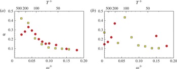
studied, and is expected to behave similarly to that of wall oscillation. As shown in figure 12(a), the wall oscillation and stationary wave display a similar trend when a relationship of
 ${\it\omega}^{+}={\it\kappa}_{x}^{+}U_{c}^{+}$
is used to find an equivalent
 ${\it\omega}^{+}$
value for
 ${\it\kappa}_{x}^{+}$
, where
 $U_{c}^{+}=10$
(Viotti et al.
Reference Viotti, Quadrio and Luchini2009). The scaling around the region of optimal drag reduction for the stationary wave is better than for the wall oscillation hinting that, at higher Reynolds number, the stationary wave may remain as a more advantageous control method within the control parameters studied.
Reynolds number scaling parameter
 ${\it\alpha}$
for (a) wall oscillation and stationary wave and (b) travelling waves (
 ${\it\kappa}_{x}^{+}=0.008$
and
 ${\it\omega}^{+}=0.06$
). An equivalent
 ${\it\omega}^{+}$
value (squares, yellow online) is calculated for
 ${\it\kappa}_{x}^{+}$
using a relationship of
 ${\it\omega}^{+}={\it\kappa}_{x}^{+}U_{c}^{+}$
, where
 $U_{c}^{+}=10$
(Viotti et al.
Reference Viotti, Quadrio and Luchini2009).

Figure 12(b) and table 5 show the
 ${\it\alpha}$
values of the scalings calculated for the travelling wave, emphasising the variation of the scaling dependent on the control parameters. Again, an equivalent
 ${\it\omega}^{+}$
values are calculated for
 ${\it\kappa}_{x}^{+}$
using
 ${\it\omega}^{+}={\it\kappa}_{x}^{+}U_{c}^{+}$
. Like the wall oscillation and stationary wave,
 ${\it\alpha}$
values vary significantly depending on
 ${\it\omega}^{+}$
and
 ${\it\kappa}_{x}^{+}$
values. The scaling is better (i.e. smaller
 ${\it\alpha}$
values) for larger
 ${\it\omega}^{+}$
and
 ${\it\kappa}_{x}^{+}$
. The main impact of this is that, although the
 ${\mathcal{D}}{\mathcal{R}}$
is reducing as the Reynolds number increases, and the scaling is strong at the optimal control parameters, by adjusting the control parameters correctly, the scaling with Reynolds number is improved. This means that, at a higher value of
 $\mathit{Re}_{{\it\tau}}$
, using the parameters which were not optimal at a low Reynolds number can give a more favourable drag reduction. In the wall oscillation and stationary wave cases, lower values of
 ${\it\omega}^{+}$
and
 ${\it\kappa}_{x}^{+}$
have higher
 ${\it\alpha}$
values, hence the drag reduction deteriorates more rapidly as the Reynolds number increases.
The
 ${\mathcal{D}}{\mathcal{R}}$
scalings for (a) the horizontal line through the map with
 ${\it\kappa}_{x}^{+}=0.008$
and (b) the vertical line with
 ${\it\omega}^{+}=0.02$
. Here
 $\dagger$
indicates the optimal parameter at
 $\mathit{Re}_{{\it\tau}}=200$
and
 $\ddagger$
indicates the optimal parameter at
 $\mathit{Re}_{{\it\tau}}=800$
.

4.4. Turbulence statistics
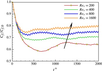
Figure 13 shows the initial response of the skin friction to the wall oscillation, normalised by
 $C_{f,0}$
. The level of oscillation in
 $C_{f}$
is seen to increase as the Reynolds number is increased while the overall drag reduction deteriorates with the Reynolds number. It has been shown that, when the oscillation is applied for large time periods (corresponding to small
 ${\it\omega}^{+}$
), substantial oscillations occur in the skin friction (Jung et al.
Reference Jung, Mangiavacchi and Akhavan1992; Touber & Leschziner Reference Touber and Leschziner2012). This is due to the turbulence responding to the wall motion, and an increase of turbulent intensity in the new shear direction. At certain points throughout the oscillation drag is increased, and this can lead to an overall drag increase when
 ${\it\omega}^{+}$
is sufficiently small (figure 4 when
 ${\it\omega}^{+}=0.01$
). Figure 13 suggests that the oscillation in the drag reduction does not scale with wall units, and deteriorates the drag reduction achieved at the optimal parameters as the Reynolds number increases. Another interesting point from this figure is that the rate of the initial decay in
 $C_{f}$
is very similar at all Reynolds numbers. However, this decay is sustained for longer at the lower Reynolds numbers; for the
 $\mathit{Re}_{{\it\tau}}=200$
case the initial decrease of
 $C_{f}$
is sustained until
 $t^{+}=700$
while the
 $C_{f}$
minimum is achieved much earlier at
 $t^{+}=300$
for the
 $\mathit{Re}_{{\it\tau}}=1600$
case. In global units, the initial decay of
 $C_{f}$
is even faster at higher Reynolds numbers.
Initial response of skin friction (normalised by the no-control case) for the wall oscillation with
 ${\it\omega}^{+}=0.06$
at the four Reynolds numbers. The arrow indicates the increase in Reynolds number:
 $\mathit{Re}_{{\it\tau}}=200,400,800$
and 1600.

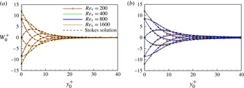
Stokes layer for oscillation case: (a)
 ${\it\omega}_{\mathit{opt}}^{+}=0.06$
(
 $T^{+}=100$
) and (b)
 ${\it\omega}^{+}=0.03$
(
 $T^{+}=200$
). Dashed lines are the laminar Stokes layer solution:
 $W(y,t)=A\text{e}^{-{\it\eta}}\cos ({\it\omega}t-{\it\eta})$
, here
 ${\it\eta}=y\sqrt{{\it\omega}/2{\it\nu}}$
.

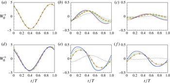
Figures 14 and 15 show the phase-averaged spanwise velocity profiles for the wall oscillation at two oscillation frequencies,
 ${\it\omega}^{+}=0.06$
(
 $T^{+}=100$
) and
 ${\it\omega}^{+}=0.03$
(
 $T^{+}=200$
). Also included are the laminar Stokes flow profiles (Schlichting Reference Schlichting1968). Please note that the laminar Stokes layer thickness is
 ${\it\delta}^{+}=\sqrt{4{\rm\pi}T^{+}}$
in wall units;
 ${\it\delta}^{+}=35.4$
for
 ${\it\omega}_{\mathit{opt}}^{+}=0.06$
(
 $T^{+}=100$
) and
 ${\it\delta}^{+}=50.1$
for
 ${\it\omega}^{+}=0.03$
(
 $T^{+}=200$
), and there is no Reynolds number dependence. For the optimal case (
 ${\it\omega}_{\mathit{opt}}^{+}=0.06$
), the spanwise turbulent velocity profiles at
 ${\it\eta}=1$
, corresponding to
 $y_{0}^{+}=6$
, are very similar to the Stokes profile at all four Reynolds numbers (figure 15
a), indicating that the turbulent Stokes layer near the wall is not affected by increasing the Reynolds number. This finding is interesting considering the weakened drag reduction observed at higher Reynolds numbers. Further away from the wall (
 ${\it\eta}=4.6$
and
 $2{\rm\pi}$
) (figure 15
b,c), the spanwise turbulent velocity decays slower than the laminar flow, and the phase difference for different Reynolds numbers is clearly discernible. At
 ${\it\omega}^{+}=0.03$
(
 $T^{+}=200$
), the spanwise turbulent velocity profile decays much slowly, and this trend was also observed in the previous DNS study at
 $\mathit{Re}_{{\it\tau}}=200$
(Touber & Leschziner Reference Touber and Leschziner2012). The Reynolds number effect is more evident at the lower
 ${\it\omega}^{+}$
value, and the spanwise turbulent velocity profile deviates significantly from the Stokes profile in figure 15(d–f). The deviation from the laminar Stokes profile increases at higher Reynolds numbers.
Phase-averaged spanwise velocity for oscillation case for (a–c)
 ${\it\omega}_{\mathit{opt}}^{+}=0.06$
(
 $T^{+}=100$
) and (d–f)
 ${\it\omega}^{+}=0.03$
(
 $T^{+}=200$
). In (a,d)
 ${\it\eta}=1$
; in (b,e)
 ${\it\eta}=4.6$
; and in (c, f)
 ${\it\eta}=2{\rm\pi}$
. Dashed lines are the laminar Stokes layer solution.

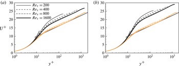
Mean velocity (
 $U^{+}$
) profiles at four Reynolds numbers. (a) Wall oscillation for
 ${\it\omega}_{\mathit{opt}}^{+}=0.06$
and (b) stationary wave cases for
 ${\it\kappa}_{x,\mathit{opt}}^{+}=0.008$
. Here
 $u_{{\it\tau}}$
is used in wall units. Black lines represent the flow control case and grey (orange) lines represent the no-control case. The thick grey straight line represents the law of the wall:
 $u^{+}=(1/{\it\kappa})\ln y^{+}+3.7$
and
 ${\it\kappa}=0.37$
(Nagib & Chauhan Reference Nagib and Chauhan2008).

The mean velocity profiles are shown in figure 16 for both the wall oscillation and stationary wave cases. The optimal control parameters are considered here:
 ${\it\omega}_{\mathit{opt}}^{+}=0.06$
(
 $T^{+}=100$
) for the wall oscillation and
 ${\it\kappa}_{x,\mathit{opt}}^{+}=0.008$
(
 ${\it\lambda}^{+}=800$
) for the stationary wave cases. For the no-control cases, the streamwise mean velocity profiles at four Reynolds numbers agree well with the log-law profile. Also included in the figure is a logarithmic velocity distribution
 $u^{+}=(1/{\it\kappa})\ln y^{+}+B$
, where
 ${\it\kappa}=0.37$
and
 $B=3.7$
(Nagib & Chauhan Reference Nagib and Chauhan2008). When the
 $u_{{\it\tau}}$
value for each controlled flow is used in wall units, the log-law velocity profiles show a characteristic upward shift (Choi et al.
Reference Choi, DeBisschop and Clayton1998; Touber & Leschziner Reference Touber and Leschziner2012), and the magnitude of the shift is roughly proportional to
 ${\mathcal{D}}{\mathcal{R}}$
. It is interesting to note that the upward shift was much larger for the stationary wave reflecting larger
 ${\mathcal{D}}{\mathcal{R}}$
values achieved. The upward shift for the wall oscillation is approximately
 ${\rm\Delta}U^{+}=5.3,3.8,3.1$
and 2.7 at
 $\mathit{Re}_{{\it\tau}}=200,400,800$
and 1600, respectively while the upward shift is larger for the stationary wave with
 ${\rm\Delta}U^{+}=7.6,6.2,5.5$
and 5.0 at
 $\mathit{Re}_{{\it\tau}}=200,400,800$
and 1600, respectively. Since the mass flow rates are constant for the uncontrolled and controlled flows, a large
 ${\rm\Delta}U^{+}$
means a thicker viscous sublayer in the controlled flow. For the stationary wave, the viscous sublayer is more affected than the wall oscillation case.
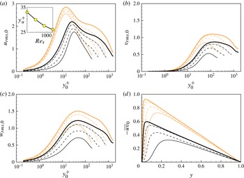
Figure 17 shows the velocity fluctuations (
 $u_{i,rms}/u_{{\it\tau}0}$
) and the Reynolds shear stress (
 $-\overline{uv}/u_{{\it\tau}_{0}}^{2}$
) for the stationary wave. The optimal wave number
 ${\it\kappa}_{x}^{+}=0.008$
is chosen for all four Reynolds numbers studied. When scaled with the friction velocity of the no-control case,
 $u_{{\it\tau}0}$
, the velocity fluctuations display two distinctive characteristics: first, all three velocity components decrease significantly, and second, the location for the maximum
 $u_{i,rms}^{+}$
moves away from the wall. A similar trend was also observed in other types of flow control (Choi, Moin & Kim Reference Choi, Moin and Kim1994; Chung & Talha Reference Chung and Talha2011). The decrease in
 $u_{rms}^{+}$
is much larger at lower Reynolds numbers, consistent with the amount of drag reduction observed earlier. As the Reynolds number increases, the effect on the velocity fluctuations becomes weaker. This can be most clearly seen in
 $u_{rms}^{+}$
profiles; for the no-control case, the maximum
 $u_{rms}^{+}$
increases by 0.3 when the Reynolds number increases from
 $\mathit{Re}_{{\it\tau}}=200$
to 1600, but the difference becomes much larger for the stationary wave with
 ${\rm\Delta}u_{rms}^{+}=0.45$
, indicating the stationary wave decreases
 $u_{rms}^{+}$
more significantly at lower Reynolds numbers. The difference between the new location for the maximum
 $u_{i,rms}^{+}$
and the no-control value is found to be quite large at
 $\mathit{Re}_{{\it\tau}}=200$
, but this reduces following
 $y_{u}^{+}\sim \mathit{Re}_{{\it\tau}}^{-0.15}$
as the Reynolds number increases.
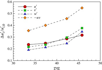
The changes in the maximum value of each component of Reynolds stresses are examined at four Reynolds numbers. The reduction in maximum
 $u_{i,rms}$
, normalised by the maximum
 $u_{i,rms}$
value for the no-control case is shown in figure 18. All quantities show good correlation with
 ${\mathcal{D}}{\mathcal{R}}$
: a large
 ${\mathcal{D}}{\mathcal{R}}$
is accompanied with a large reduction in the maximum value of the Reynolds stresses. Chung & Talha (Reference Chung and Talha2011) observed a similar trend in the opposition control. This finding shows that turbulence fluctuations (e.g.
 $u_{rms}$
) are reduced much less by the flow control at higher Reynolds numbers. Iwamoto et al. (Reference Iwamoto, Fukagata, Kasagi and Suzuki2005) suggested that the degree of turbulence attenuation in the near-wall region is related to the amount of drag reduction achievable. This may explain why drag reduction deteriorates at high Reynolds numbers.
Reynolds stresses profiles from the stationary wave cases for
 ${\it\kappa}_{x,\mathit{opt}}^{+}=0.008$
at four Reynolds numbers: (a)
 $u_{rms}^{+}$
, (b)
 $v_{rms}^{+}$
, (c)
 $w_{rms}^{+}$
and (d)
 $-\overline{uv}$
. Here
 $u_{{\it\tau}0}$
is used in wall units. Black lines represent the flow control case, and grey (orange) lines represent the no-control case. The inset in (a) is for the location of the maximum
 $u_{rms}^{+}$
for the stationary wave cases in log–log scale,
 $y_{u}^{+}\sim \mathit{Re}_{{\it\tau}}^{-0.15}$
.

Reduction in maximum
 $u_{i,rms}$
as a function of
 ${\mathcal{D}}{\mathcal{R}}$
,
 ${\rm\Delta}u_{i,\mathit{max}}/u_{i,\mathit{max},0}$
. Here
 ${\rm\Delta}u_{i,\mathit{max}}$
is normalised by the maximum
 $u_{i,rms}$
value for the no-control case,
 $u_{i,\mathit{max},0}$
.

Since the drag reduction is directly related to the Reynolds shear stress,
 $-\overline{uv}$
profiles are analysed further. Fukagata, Iwamoto & Kasagi (Reference Fukagata, Iwamoto and Kasagi2002) showed that the contribution of the Reynolds shear stress to the skin-friction drag is the weighted average of Reynolds shear stress.
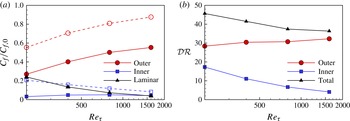
 $$\begin{eqnarray}C_{f}=\frac{6}{\mathit{Re}}+6\int _{0}^{1}\left(1-y\right)(-\overline{uv})\text{d}y,\end{eqnarray}$$
where
 $\mathit{Re}=U_{m}h/{\it\nu}$
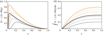
. The first term is the laminar flow contribution while the second term represents the turbulent flow contribution. Figure 19(a) shows the
 $(1-y)(-\overline{uv})$
profile for four Reynolds numbers. The accumulated contribution of the weighted turbulent shear stress from 0 to
 $y$
is shown in figure 19(b). The Reynolds shear stress in figures 17(d) and 19(a) shows a stronger Reynolds number effect. This is not surprising because the no-control turbulent flow also experiences the Reynolds number effect close to the wall (DeGraaff & Eaton Reference DeGraaff and Eaton2000; Hoyas & Jiménez Reference Hoyas and Jiménez2006).
(a) Weighted turbulent shear stress,
 $\left(1-y\right)(-\overline{uv})$
, and (b) accumulated contribution of the weighted turbulent shear stress from 0 to
 $y$
,
 $\int _{0}^{y}\left(1-y\right)(-\overline{uv})\text{d}y$
.

In this study, the turbulent flow contribution is further divided into two components: inner and outer regions. The wall-normal location for the maximum of the Reynolds shear stress,
 $y_{\text{p}}$
, is used
 $$\begin{eqnarray}C_{f}=\frac{6}{\mathit{Re}}+6\left[\int _{0}^{y_{\text{p}}}\left(1-y\right)(-\overline{uv})\text{d}y+\int _{y_{\text{p}}}^{1}\left(1-y\right)(-\overline{uv})\text{d}y\right],\end{eqnarray}$$
Sreenivasan & Sahay (Reference Sreenivasan, Sahay and Panton1997) argued that the momentum balance in the critical layer around
 $y_{\text{p}}$
is different from those in the classical inner and outer layers. It is known that the
 $y_{\text{p}}^{+}$
location increases with the Reynolds number:
 $y_{\text{p}}^{+}=2\mathit{Re}_{{\it\tau}}^{1/2}$
(Sreenivasan & Sahay Reference Sreenivasan, Sahay and Panton1997; Guala, Hommema & Adrian Reference Guala, Hommema and Adrian2006).
Figure 20(a) shows that for no-control case, the contribution of the outer region increases with the Reynolds number while the contribution of the inner region decreases gradually. As expected, the laminar contribution becomes smaller as the Reynolds number increases. For the stationary wave, the contribution of the outer region is significantly reduced at all Reynolds numbers tested, and the amount of reduction does not appear to be affected by increasing the Reynolds number, indicating a constant drag reduction from the outer region. The contribution of the inner region is roughly constant for the stationary wave. Figure 20(b) displays the contribution of each component to
 ${\mathcal{D}}{\mathcal{R}}$
. The contribution of the outer region becomes more or less constant, just over
 ${\mathcal{D}}{\mathcal{R}}\approx 30$
, while the contribution of the inner region diminishes gradually from
 ${\mathcal{D}}{\mathcal{R}}=20$
at
 $\mathit{Re}_{{\it\tau}}=200$
. The Reynolds number effect shown in figure 20(b) is related to a weaker drag reduction observed at high Reynolds numbers. This is consistent with Iwamoto et al. (Reference Iwamoto, Fukagata, Kasagi and Suzuki2005). They predicted that the Reynolds number effect on the drag reduction rate is relatively mild (i.e. logarithmic) if the fluctuations in the regions near the wall can completely be damped. This finding suggests an exciting possibility of a finite
 ${\mathcal{D}}{\mathcal{R}}$
value at a very high Reynolds number, which is very promising for the transport industry, in particular, the air transport, where a typical operating condition is of the order of
 $\mathit{Re}_{{\it\tau}}=10\,000$
. This is a conjecture at this stage, and a further study with higher-Reynolds-number DNS or experiment will be able to present a clearer picture regarding the Reynolds number effect.
(a) Skin-friction contribution from laminar component; inner and outer regions. Dashed lines with open symbols are for the no-control cases, and solid lines are for the stationary wave cases. (b) Contribution to
 ${\mathcal{D}}{\mathcal{R}}$
from inner and outer regions. The total
 ${\mathcal{D}}{\mathcal{R}}$
values are also included.

5. Conclusions
A series of DNS of a turbulent channel flow subjected to streamwise travelling waves have been performed for a Reynolds number range up to
 $\mathit{Re}_{{\it\tau}}=1600$
. Drag reduction maps are calculated from DNS results at
 $\mathit{Re}_{{\it\tau}}=200$
, 400 and 800. It is found that the maximum drag reduction achieved by travelling waves decreases significantly as the Reynolds number is increased. The intensity of both the drag reduction and drag increase is reduced with the Reynolds number. This reduction does not scale universally, and the drag reduction deteriorates rapidly with increased Reynolds number when the control parameters used are close to the optimal values found at a lower Reynolds number. It is also found that the value of the optimal control parameters (
 ${\it\omega}_{\mathit{opt}}^{+}$
and
 ${\it\kappa}_{x,\mathit{opt}}^{+}$
) changes, even in wall units, as the Reynolds number is increased. This makes approximation of the maximum drag reduction achievable at high Reynolds numbers difficult. The value of
 ${\it\omega}_{\mathit{opt}}^{+}$
for the wall oscillation and
 ${\it\kappa}_{x,\mathit{opt}}^{+}$
for the stationary wave increase with the Reynolds number.
The scaling with the Reynolds number is found to be non-trivial. A scaling in the form
 $\mathit{Re}_{{\it\tau}}^{-{\it\alpha}}$
results in a wide range of
 ${\it\alpha}$
values depending on the flow control parameters. Due to the complex
 ${\mathcal{D}}{\mathcal{R}}$
scaling it is possible that, although the drag reduction deteriorates rapidly at the optimal found at a lower Reynolds number, by choosing a non-optimal parameter, the control method may still yield reasonable values of
 ${\mathcal{D}}{\mathcal{R}}$
at a higher Reynolds number. There is no Reynolds number effect in the spanwise velocity profiles when the optimal parameter
 ${\it\omega}_{opt}^{+}$
is used, and the Stokes layer is nearly insensitive to the Reynolds number. The effect of flow control on the mean and r.m.s. velocity profiles is weakened at high Reynolds numbers as the drag reduction becomes less effective. The Reynolds shear stress analysis suggests the Reynolds number effect on the drag reduction could be rather mild, leading to a possible constant
 ${\mathcal{D}}{\mathcal{R}}$
at higher Reynolds numbers.
Acknowledgements
The research leading to these results has received support from the EPSRC (Grant EP/G060215/1), EADS UK Limited and Airbus Operations Limited, and the European Union Seventh Framework Programme FP7/2007-2013 AirPROM (Grant Agreement FP7 270194, www.airprom.eu). Q.Y. was sponsored by China Scholarship Council. We are grateful to Dr N. Li from NAG for his help with the code parallelisation process. We also would like to thank M. Quadrio for interesting discussions and suggestions. Further thanks to D. A. Lockerby, M. A. Leschziner, S. I. Chernyshenko, S. Rolston, R. Ashworth and J. J. Benton. The simulations were performed on the HPC machines (Minerva) at the Centre for Scientific Computing, University of Warwick. The support from the UK Turbulence Consortium (Grant EP/G069581/1, EP/L000261/1) is also acknowledged. This work used the HECToR and ARCHER UK National Supercomputing Service (http://www.archer.ac.uk).