2 Numerical method

The governing equations in cylindrical coordinates for incompressible, fully developed turbulent pipe flow were integrated in time using the fractional step method along with the implicit velocity decoupling procedure. Position is denoted by $\boldsymbol{x}=(x,r,\unicode[STIX]{x1D703})=(x,y,z)$ , where; $x$ is the streamwise (or axial) distance from the inlet; $r$ is the distance from the centreline; $\unicode[STIX]{x1D703}$ is the azimuthal angle; $y=R-r$ is the distance from the wall; and $z=r\unicode[STIX]{x1D703}$ is the spanwise distance. The corresponding velocity fluctuating components are $u$ ( $=u_{x}$ ), $v$ ( $=-u_{r}$ ) and $w$ ( $=u_{\unicode[STIX]{x1D703}}$ ), and $U$ is the temporally and spatially averaged (i.e. $x$ - and $\unicode[STIX]{x1D703}$ -directions) streamwise mean velocity. The maximum velocity of the fully developed laminar profile ( $U_{c}$ ) and the pipe radius ( $R$ ) were used to non-dimensionalize the equations in the numerical solution. Consequently, the unit time scale is $R/U_{c}$ . As usual, the superscript $+$ refers to quantities normalized by the friction velocity, $u_{\unicode[STIX]{x1D70F}}$ or viscous length scale $\unicode[STIX]{x1D708}/u_{\unicode[STIX]{x1D70F}}$ , and the Reynolds number $\mathit{Re}_{D}=U_{b}D/\unicode[STIX]{x1D708}$ ( $=U_{c}R/\unicode[STIX]{x1D708}$ ) is defined based on the pipe diameter, $D=2R$ , and the bulk velocity, $U_{b}$ . Numerically, $\mathit{Re}_{D}=35\,000$ , and the von Kárman number is $R^{+}=\mathit{Re}_{\unicode[STIX]{x1D70F}}=u_{\unicode[STIX]{x1D70F}}R/\unicode[STIX]{x1D708}=934$ . The streamwise domain was made $30R$ long, based on the previous experimental and numerical studies of Kim & Adrian (Reference Kim and Adrian1999) and Wu et al. (Reference Wu, Baltzer and Adrian2012). The finite-difference grid size employed in the current work is $4097\times 301\times 1025$ along the axial, radial and azimuthal directions with grid resolutions $\unicode[STIX]{x0394}x^{+}=6.84$ , $\unicode[STIX]{x0394}(R\unicode[STIX]{x1D703})^{+}=5.73$ , $\unicode[STIX]{x0394}r_{min}^{+}=0.33$ and $\unicode[STIX]{x0394}r_{max}^{+}=9.24$ . The inflow and outflow conditions were periodic, and the bulk velocity was fixed leaving the integrated wall shear stress to fluctuate. Further numerical details may be found in Lee & Sung (Reference Lee and Sung2013).

3 Time-evolving instantaneous fields

The primary question in the present study is how a VLSM is created in the flow. The idea that small scales organize to create larger scales is quite reasonable, and it has received increasing support over the past decade (Adrian Reference Adrian2007). The hairpin packet model, which consists of hairpin vortices aligned in a streamwise linear fashion offers an explanation for the most fundamental features of wall turbulence, such as the multiple second quadrant bursting process, sweeps, the growth of length scale with increasing distance from the wall, and the occurrence of low-momentum zones (Meinhart & Adrian Reference Meinhart and Adrian1995; Adrian et al. Reference Adrian, Meinhart and Tomkins2000; Adrian Reference Adrian2007). Further, the creation of the first generation of hairpin packets in the region above the buffer layer, as explained by the auto-generation mechanism (Zhou et al. Reference Zhou, Adrian, Balachandar and Kendall1999), is an established mechanism in which hairpins with sufficient strength create more new hairpins, and so on, ultimately forming relatively coherent packets. Evidence from prior investigations (Marusic & Adrian Reference Marusic and Adrian2012) supports the idea that the tall low-momentum zones identified as LSMs (in their figures 2–4) are among the oldest and largest packets that result from a hierarchy of streamwise and spanwise mergers starting with the first generation of packets auto-generated above the buffer layer. They are the analogues of bulges found in turbulent boundary layers.

Figure 1.

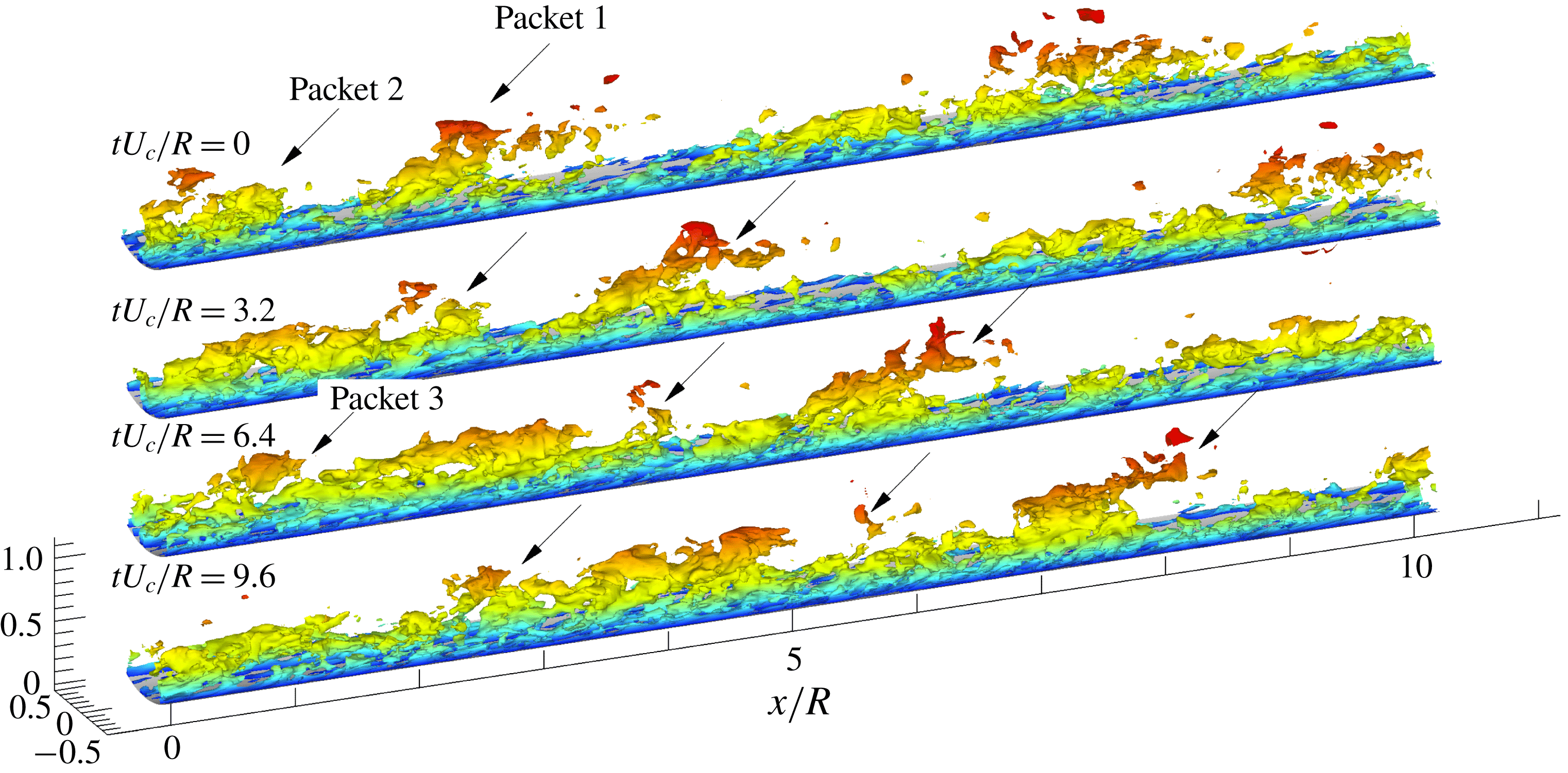
Three-dimensional isocontour of the streamwise velocity fluctuating structures with the contour level of $u^{+}=-2$ . The flow direction is from left to right. The isosurfaces are coloured based on the local value of $y/R$ with higher $y/R$ represented in red.

A hairpin induces negative velocity (with respect to the hairpin) in the region under its head and between its neck and legs. Inside a packet of hairpins a long low-momentum zone is formed owing to the in-line alignment of the hairpins. The ramp-shape of the low-momentum zone mimics the shape of the envelope of the hairpin packet, albeit in a smoothed manner, and it is recognized readily because the height of the envelope increases in the downstream direction along a characteristic ramp angle in the range $10^{\circ }$ – $15^{\circ }$ (pertaining to the logarithmic layer), presenting a ramp-like low-momentum zone when viewed from the side. As the hairpin packets grow they encounter other packets (Adrian, Balachandar & Liu Reference Adrian, Balachandar and Liu2001; Tomkins & Adrian Reference Tomkins and Adrian2003) leading to considerable scrambling of the vortices. For this reason it proves convenient in this study to use contours of low velocity to identify hairpin packets, as in Dennis & Nickels (Reference Dennis and Nickels2011), Lee & Sung (Reference Lee and Sung2011), Baltzer et al. (Reference Baltzer, Adrian and Wu2013) and Lee (Reference Lee2017).

The 3-D visualization of typical very long low-speed structures in figure 1 uses a contour level of $u^{+}=-2$ . The streamwise extent of the figure is $10R$ , and the azimuthal range is shown in the right corner. Three very long low-speed streaks that are slightly inclined to the spanwise direction are shown with lengths in excess of the entire field of view in the flow direction, and with characteristic widths of approximately $0.5R$ in the spanwise direction. These structures extend downwards to the near-wall region, consistent with the ‘footprints’ described by Hutchins & Marusic (Reference Hutchins and Marusic2007a ) for modulation of small-scale structures in the near-wall region. They also extend upwards through the outer layer and almost to the centreline of the pipe (see the colour contour).

Figure 2.

Perspective visualization of the time-evolving instantaneous low-momentum zones. The contour level is $u^{+}=-2$ , and the flow direction is from left to right. The colour legend is identical to that in figure 1.

Figure 3.

Top view of the time-evolving low-momentum zones. The contour level is $u^{+}=-2$ , and the flow direction is from left to right. The ellipses indicate the LSMs. The colour legend is identical to that in figure 1. The solid line at $tU_{c}/R=9.6$ indicates approximate centre position of the LSMs at each streamwise location.

Figure 4.

Evidence for the formation of VLSM through merging of LSMs. The black contours indicate the low-momentum regions ( $u^{+}=-1.0$ ). The data here are extracted along the streamwise-aligned dashed lines in figure 3. Solid lines indicate the approximate envelopes of the packets, and dashed lines are visible to show the streamwise trajectories of the travelling near-wall (thin) and outer layer (bold) structures.

Figures 2 and 3 present time-evolutions of the 3-D flow field in the perspective and top views to show how VLSM 1 in figure 1 is created (VLSM 1 in figure 1 corresponds to $tU_{c}/R=9.6$ in figures 2–4). The contour level is $u^{+}=-2$ , and the time interval is $tU_{c}/R=3.2$ . Figure 4, showing temporal variation of the low-momentum regions in the $x$ – $y$ plane, completes the visualization. The data were extracted along the fixed spanwise location (horizontal dashed line) in figure 3, and the contour is adjusted to $u^{+}=-1.0$ for clarity. At the initial time $tU_{c}/R=0$ , there are two adjacent ramp-like structures in figures 3 and 4, packet 2 ( $x/R<1.2$ ) and packet 1 $(1.5<x/R<3.5)$ having lengths of $2{-}3R$ . These packets are LSM structures. They are inclined at angles of approximately $15^{\circ }{-}25^{\circ }$ to the wall, and they are presumably the oldest and largest packets because they extend over a substantial region of the pipe core, typically up to $0.6R$ . Smaller, younger packets can also be seen, and to distinguish them from the largest packets we shall refer to the smaller packets simply as packets. Note that the angle of the LSM packet ramps is larger than the $10^{\circ }$ – $15^{\circ }$ mean angle of first generation packets (Christensen & Adrian Reference Christensen and Adrian2001; Adrian Reference Adrian2007). The reason will be described later. LSM packets 1 and 2 evolve slowly in time, moving with almost equal convection velocities along the downstream direction (figures 2–4). Because the outermost regions of packets 1 and 2 (corresponding to the heads or arches of the tallest hairpins) experience higher mean flow velocity than the lower regions, they move downstream faster than the lower-lying regions of the packets, as can be seen in figure 4, wherein bold and thin dashed lines connect high and low parts of the ramp-like low-momentum zones of packets 1 and 2 at four times. Their slopes indicate approximate convection velocities, and they closely match with the mean velocities at $y/R=0.02$ and 0.35. This process results in two kinematic phenomena: (a) within each LSM packet the taller hairpins move downstream faster than the shorter hairpins, resulting in elongation of each packet; and (b) the heads of the hairpins move faster than their lower parts (necks and legs), resulting in shearing motion. Since shear is a combination of rotation and plane strain with stretching at $45^{\circ }$ to the mean flow, inclined hairpin vortices in the packets must be intensified by stretching and inclined forward by the rotation. As time increases the stretching of LSM packets 1 and 2 is clear in figure 4.

The tallest part of packet 2 (that appears to be a detached structure) overruns the near-wall part of packet 1 (figure 4), which moves more slowly in the streamwise direction. Eventually, the head of the upstream LSM packet 2 merges with the tail of the downstream LSM packet 1, the connection first beginning close to the wall and later extending beyond the logarithmic layer (see figure 2). At $tU_{c}/R=6.4$ , the tallest part of packet 2 starts to settle down into the valley-like region between the adjacent ramp-like low-momentum patterns, and the continuous interaction of the structures results in the connection of the packets at $tU_{c}/R=9.6$ , creating the longer structure of the VLSM. Lee et al. (Reference Lee, Lee, Choi and Sung2014) showed that the convection velocity of the low-speed region is lower than the mean streamwise velocity, whereas the velocity in the high-speed region exceeds the mean streamwise velocity. In addition, they found that the convection velocity depends on the strength of the velocity fluctuations, i.e. it is increased with an increase of the strength in the velocity fluctuations. As a result, these differences of the convection velocity lead to the concatenation between in-line low-speed structures. In figure 4, the connecting structure residing in the valley seems to be trapped between the packet 1 and 2 for a long time, presumably because it cannot travel downstream due to packet 1. As a result, the VLSM maintains its coherence for a relatively long time.

After $tU_{c}/R=9.6$ , the adjacent packets 1 and 2 are completely merged at the downstream, and they form a long, but hardly straight, low-momentum zone travelling in the streamwise direction (figure 3). The pattern gives an appearance of meandering, but this is caused by the lateral offset of the merging packets, not by temporal spanwise oscillations. The merged low-momentum zone appears to make a smaller angle with respect to the wall (figure 4) owing to its length being approximately doubled without a concomitant increase in height.

In addition to the stretching, shearing and merging process, we have also found examples in the database where VLSM longer than $3R$ begins as a single structure (shorter than $3R$ ) and grows much longer without merging. However, this type of event occurs infrequently in our DNS dataset, and the merging event shown in figures 2–4 is the primary mechanism by which scales of motion larger than the LSMs formed. Statistical evidence indicating the commonplace occurrence of this mechanism will be provided later.

At $tU_{c}/R=6.4$ in figures 2–4, another LSM packet-like structure (packet 3 designated by the arrow in figures 2 and 3) appears further upstream. Due to its spanwise-offset (see figure 3), packet 3 is not visible in figure 4 at $tU_{c}/R=9.6$ . Therefore, the upstream end of packet 2 observed at $tU_{c}/R=0.0$ and 3.2 is probably a small portion of merged structure between LSM packets 2 and 3, and additional merging occurs with the downstream LSM packet 1. This is another indication of the commonplace nature of mergers leading to longer structures. Consistent with our observation, Lee et al. (Reference Lee, Lee, Choi and Sung2014) reported that in a turbulent channel flow the streamwise merging event between the LSMs is frequently observed near the wall, although the frequency of the merging event decreases far from the wall. The dominance of the merging event near the wall suggests that the energetic peak of the VLSMs in energy spectrum occurs near the wall compared to the LSMs (Monty et al. Reference Monty, Hutchins, Ng, Marusic and Chong2009).

The overall picture is consistent with the finding of Lee & Sung (Reference Lee and Sung2011), who studied the VLSM formation mechanism in the time-evolving fields of a boundary layer using DNS. Examination of the video of the spatially developing turbulent boundary layer on a flat plate made by Lee et al. (Reference Lee, Kwon, Hutchins and Monty2012) also shows merging between large packets in the manner just described. Furthermore, the signature of the velocity fluctuations by Kevin, Monty & Hutchins (Reference Monty and Hutchins2019) with a VLSM pattern is consistent with our observation, although they described the VLSM pattern using meandering. Thus, it has the potential to be a root cause of VLSM with a helical angle that is observed in significantly different outer flow geometry.

The streamwise concatenation process should not be confused with the near-wall auto-generation mechanism, which also creates longer sequences of hairpin eddies. Auto-generation is an organic growth process, whereas concatenation is mainly a simple piecing together (although interactions between the vortices of the merging LSMs may, and probably do occur).

The top view in figure 3 confirms that the very long structure at $tU_{c}/R=9.6$ is not perfectly aligned along the streamwise direction, but inclined to the spanwise direction with negative azimuthal angle (see solid line). However, it should be noted that the primary body of LSM packet at $tU_{c}/R=0.0$ and 3.2 tilts with positive spanwise-inclination angle. As LSM packet 1 merges with upstream LSM packet 2 at $tU_{c}/R=6.4$ and 9.6, the upstream body of packet 1 alters its inclination from positive to negative (from downward to upward), and the two LSM packets concatenate with a very shallow angle. In this figure (at $tU_{c}/R=9.6$ ), the inclined angle of the total VLSM is approximately $4^{\circ }$ , in agreement with Baltzer et al. (Reference Baltzer, Adrian and Wu2013). They suggested that as the packet-like entities concatenate in streamwise succession, there is also azimuthal offset of the LSMs with a dominant helical angle. In order to examine how the helical pattern of the VLSM is created in the present study, we considered the time-evolving instantaneous fields with larger field of view (not shown here). The result showed that packet 3 exists with a larger azimuthal offset than packet 2, and the continuous merging of packet 3 with the downstream packet creates a long low-momentum zone aligned along a helical path. The angle of the helical VLSM is determined by the pattern of the LSMs, i.e. the axial and azimuthal offsets prior to merger. The LSMs that are aligned without offset can form a VLSM having vanishing helical angle. The length of the VLSM also depends on the initial pattern of LSMs. For example, despite packet 1 stretching continuously, it does not encounter downstream packets that are old and large to be merger partners, and no additional mergers are observed out to $tU_{c}/R=9.6$ .

While the growth and alignment of spanwise-offset LSMs explains the formation of helical low-speed streaks on the VLSM scale, our understanding of the origin of VLSMs will not be complete until the genesis of the offset alignment is explained. Ultimately, the final explanation must rest on a dynamical model that embodies the interaction of the different scales and shows how they evolve to a statistical equilibrium that contains the observed patterns and alignments. Such a model is not within the scope of this paper. Instead, we will attempt to document the patterns in both the VLSM and the LSM, and show how they are related.

4 Statistical analysis

If the formation mechanism observed in the instantaneous fields is a common occurrence, it must leave an imprint on the two-point spatial correlation coefficient of the streamwise velocity fluctuations, $R_{uu}$ , defined as

(4.1) $$\begin{eqnarray}R_{uu}(r_{x},r,r_{\unicode[STIX]{x1D703}};r_{ref})=\langle u(x,r_{ref},\unicode[STIX]{x1D703},t)u(x^{\prime },r,\unicode[STIX]{x1D703}^{\prime },t)\rangle /\unicode[STIX]{x1D70E}_{u}(r_{ref})\unicode[STIX]{x1D70E}_{u}(r),\end{eqnarray}$$

where $\unicode[STIX]{x1D70E}_{u}$ denotes the root mean square value of $u$ . Since fully developed, axisymmetric pipe flow is homogeneous in the $x$ - and $\unicode[STIX]{x1D703}$ -directions, $R_{uu}$ depends only on the spatial separations $r_{x}=x^{\prime }-x$ and $r_{\unicode[STIX]{x1D703}}=\unicode[STIX]{x1D703}^{\prime }-\unicode[STIX]{x1D703}$ . The brackets $\langle \cdot \rangle$ denote an average over time and $x$ - $\unicode[STIX]{x1D703}$ . Figure 5 plots contours of $R_{uu}$ in the $r_{x}{-}r_{z}$ plane at $y_{ref}/R=0.15$ , where $r_{z}$ is the separation in the $z$ -direction denoted by $r_{z}=(R-y)r_{\unicode[STIX]{x1D703}}$ . It shows an approximately $7R$ long region of positive correlation flanked by shorter regions of negative correlation on both sides in the spanwise direction. For the purpose of validation, isocorrelation contours for the present simulations are compared to the correlation found by Baltzer et al. (Reference Baltzer, Adrian and Wu2013) at $\mathit{Re}_{\unicode[STIX]{x1D70F}}=685$ . The agreement is reassuring, considering the differences in the DNS codes and Reynolds number.

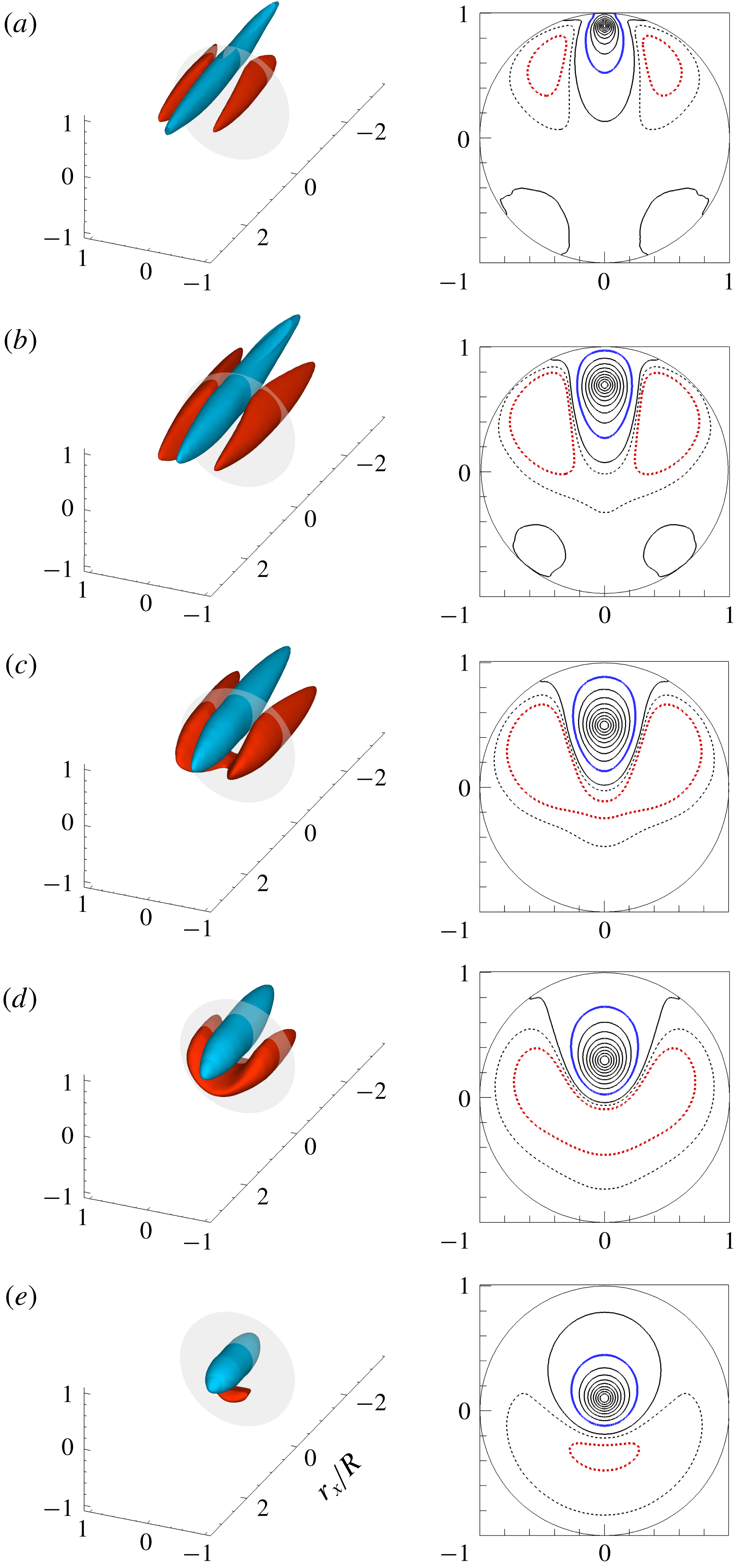
Figure 6 shows 3-D views of $R_{uu}$ and two-dimensional (2-D) contours in the cross-stream plane ( $r_{x}=0$ ) for various wall-normal reference locations. Above $y_{ref}/R=0.3$ , the highly elongated region of positive correlation is bracketed above and to the side by two long, anti-correlated regions, a space–time averaged manifestation of the high-momentum zones surrounding low-momentum zones in the instantaneous fields. The ramp-like contours of the positive correlations in the logarithmic layer are a common feature in turbulent boundary layers (Hutchins & Marusic Reference Hutchins and Marusic2007a ; Lee & Sung Reference Lee and Sung2011) and turbulent pipe flow (Baltzer et al. Reference Baltzer, Adrian and Wu2013), and we interpret them to be consequences of the low-momentum zones inside long hairpin packets.

Figure 5.

Contour lines of correlation coefficient $R_{uu}$ in the $r_{x}{-}r_{z}$ plane, with the reference point at $y_{ref}/R=0.15$ . Black lines are from the present DNS data, and dashed lines indicate negative values. Red lines from correlation contours found by Baltzer et al. (Reference Baltzer, Adrian and Wu2013) are included for validation.

Contours in the cross-sectional planes in figure 6(a,b) reveal weak, but significant, positive correlation between the reference location at $0^{\circ }$ and locations centred at ${\sim}140^{\circ }$ and ${\sim}220^{\circ }$ . The proximities of these correlation maxima to $140^{\circ }$ and $220^{\circ }$ , suggest a three-wavelength Fourier mode in the $\unicode[STIX]{x1D703}$ -direction. This result is contrary to the hot-wire experiment of Bailey et al. (Reference Bailey, Hultmark, Smits and Schultz2008), who found no apparent correlation outside $|\unicode[STIX]{x1D703}|<90^{\circ }$ from the reference location. They concluded that long structures are not periodic in the azimuthal direction and that the interaction between the motions on the opposing sides of the pipe is minimal. Results from a POD of the present flow show long, energetic modes including 0, 1, 2, 3 and more wavelengths in $\unicode[STIX]{x1D703}$ . Summation of modes needed to construct the above correlation function could pull the location of the secondary positive maxima in figure 6(a,b) closer to $140^{\circ }$ and $220^{\circ }$ , perhaps explaining the slightly non-periodic spacing in $\unicode[STIX]{x1D703}$ . As the reference height is increased, the two red, anti-correlated regions gradually merge because the spanwise (or azimuthal) domain $(z=r\unicode[STIX]{x1D703})$ decreases with increasing wall-normal height, even as their spanwise length scale increases.

Figure 6.

Correlation coefficient $R_{uu}$ in 3-D perspective view. The 2-D slices on the transparent cross-stream plane at $r_{x}/R=0$ are shown on the right-hand side. Reference points are located at (a) $y_{ref}/R=0.1$ , (b) $y_{ref}/R=0.3$ , (c) $y_{ref}/R=0.5$ , (d)  $y_{ref}/R=0.7$ , (e) $y_{ref}/R=0.9$ . Isocontour levels for the 3-D view are $R_{uu}=0.1$ (blue) and $-0.05$ (red), and contour spacing for the 2-D view is varied from 0 to 1.0 with an interval of 0.1 including $-0.025$ and $-0.05$ . In the 2-D view, thick blue and red lines indicate $R_{uu}=0$ .1 and $-0.05$ corresponding to the isosurfaces in 3-D view.

The two-point spatial correlation function averages the structural characteristics of eddies over all scales. Since our interest is in typical individual structures of the VLSM and LSM, we will divide $u$ into two signals associated with the significantly different lengths of the VLSMs and LSMs and compute correlations of each to ascertain the spatial structures of the large and very large motions. Various approaches have been used to separate the motions, most using a sharp cut at a streamwise wavenumber demarcating the VLSM from the LSM. Figure 7 compares the pre-multiplied one-dimensional streamwise energy spectrum from our simulation with DNS data at the lower Reynolds number ( $\mathit{Re}_{\unicode[STIX]{x1D70F}}=685$ ) at $y_{ref}/R=0.1$ (Wu et al. Reference Wu, Baltzer and Adrian2012). Further, an experimental pipe spectrum measured by Kim & Adrian (Reference Kim and Adrian1999) at $\mathit{Re}_{\unicode[STIX]{x1D70F}}=825$ is included, although this spectrum was not published in Kim & Adrian (Reference Kim and Adrian1999). The experimental spectrum (red dashed line) clearly shows the bimodal shape characteristics in the logarithmic layer and there are two clear peaks in the experimental spectrum at $k_{x}R\sim 1$ and $k_{x}R\sim 4$ , thought to indicate the VLSM and LSM, respectively. The long-wavelength peak (blue dashed line) for the DNS from Wu et al. (Reference Wu, Baltzer and Adrian2012) appears attenuated relative to the experimental spectrum, but the present spectrum at the high Reynolds number (solid line) suggests that a long-wavelength peak occurs at long wavelength $(k_{x}R\sim 0.8{-}0.9)$ . Relative to the spectrum of our numerical simulation, the experimental peak at long wavelength is amplified despite of the low Reynolds number, an effect caused by the use of Taylor’s hypothesis according to the theory of del Álamo & Jiménez (Reference del Álamo and Jiménez2006). Marusic & Monty (Reference Marusic and Monty2019) reported that the long-wavelength peak is associated with the type-B eddies which are physically detached eddies that are expected to scale with the boundary layer thickness. The energy of the VLSMs or superstructures consist of the contribution from the type-A eddies (attached eddies) and type-B eddies, and there remains the question of how much energy comes from an individual eddy.

Figure 7.

Pre-multiplied one-dimensional streamwise spectra $k_{x}\unicode[STIX]{x1D6F7}_{uu}/u_{\unicode[STIX]{x1D70F}}^{2}$ . Solid line: present simulation data at $y_{ref}/R=0.1$ ; red dashed line: experimental data from Kim & Adrian (Reference Kim and Adrian1999) at $y_{ref}/R=0.1$ and $\mathit{Re}_{D,cl}=33\,800$ based on the pipe diameter and turbulent centreline velocity; blue dashed line: DNS data from Wu et al. (Reference Wu, Baltzer and Adrian2012) at $y_{ref}/R=0.1$ and $\mathit{Re}_{\unicode[STIX]{x1D70F}}=685$ . The spectra for VLSM (square red symbols) and LSM (circular red symbols) are the result of decomposing the total spectrum using smooth low-pass (open squares) and high-pass (open circles) filters. The cutoff wavenumbers used to separate the VLSM from the LSM by Guala et al. (Reference Guala, Hommema and Adrian2006) at all $y_{ref}/R$ and Bailey et al. (Reference Bailey, Hultmark, Smits and Schultz2008) at $y_{ref}/R=0.2$ are shown with arrows for reference.

The wavenumber of the minimum between the two experimental peaks, at $k_{x}R\sim 1.5$ , would be a well-defined candidate to divide the VLSM velocity from the LSM velocity, except that it fails to account for the lower energy of the VLSM spectrum relative to that of the LSM spectrum (Kim & Adrian Reference Kim and Adrian1999). As noted in the introduction, Guala et al. (Reference Guala, Hommema and Adrian2006) and Balakumar & Adrian (Reference Balakumar and Adrian2007) used the slightly larger nominal value $k_{x}R=2$ as the wavenumber separating the VLSMs and the LSMs because there is a clear change in the sign of the co-spectrum of $u$ and $v$ around this value, and it corresponds to a mean wavelength of $\unicode[STIX]{x03C0}R$ that is close to the mean length of LSMs found by Kovasznay et al. (Reference Kovasznay, Kibens and Blackwelder1970). Bailey et al. (Reference Bailey, Hultmark, Smits and Schultz2008) and Bailey & Smits (Reference Bailey and Smits2010) employed wavenumbers across the range $0.6\leqslant k_{x}R\leqslant 1.5$ (depending on $y/R$ ) to divide the VLSM from LSM. The grey-shaded range in figure 7 contains all of the foregoing estimates of the wavenumber separating LSMs and VLSMs.

We have assessed the sensitivity of the respective spatial correlations to the separating wavenumber value. The magnitudes of the correlations are affected by the separating wavenumber, but spatial features, such as the scale and shape of the correlation contours are largely unaffected, in agreement with Bailey & Smits (Reference Bailey and Smits2010). Therefore, when using a sharp boundary to distinguish large from very large we have chosen the wavenumber $k_{x}R=2$ to be consistent with the work of Guala et al. (Reference Guala, Hommema and Adrian2006) and Balakumar & Adrian (Reference Balakumar and Adrian2007). Note that filtered velocities obtained using mutually exclusive filters, such as the sharp cutoff filters, must be statistically uncorrelated.

While a single, nominal wavenumber separating large- from very-large-scale motions is convenient for purposes of discussion and characterization, it is not physical, because the spectra of the VLSMs and the LSMs are certain to overlap. Moreover, taking the inverse Fourier transform of sharply cut spectra to get the correlation functions can produce unphysical ringing due to the discontinuity. Hence, separation by filtering in streamwise wavenumber space is better done with a pair of overlapping, smoothly decreasing low-pass and high-pass filters, having energy transfer characteristics such as the two curves which consist of open squares and circles in figure 7.

The two-sided co-spectrum of $u$ with streamwise wavenumber $k_{x}$ and azimuthal wavenumber $k_{\unicode[STIX]{x1D703}}$ is defined as

(4.2) $$\begin{eqnarray}S_{uu}(k_{x},r,k_{\unicode[STIX]{x1D703}};r_{ref})\equiv \frac{1}{(2\unicode[STIX]{x03C0})^{2}}\int _{-\infty }^{\infty }\,\text{e}^{-\sqrt{-1}(k_{x}r_{x}+k_{\unicode[STIX]{x1D703}}r_{\unicode[STIX]{x1D703}})}R_{uu}(r_{x},r,r_{\unicode[STIX]{x1D703}};r_{ref})\unicode[STIX]{x1D70E}_{u}(r_{ref})\unicode[STIX]{x1D70E}_{u}(r)\,\text{d}r_{x}\,\text{d}r_{\unicode[STIX]{x1D703}}.\end{eqnarray}$$

If $u_{vl}$ is obtained by passing $u$ through a low-pass filter $H_{vl}(k_{x})$ its co-spectrum is

(4.3) $$\begin{eqnarray}S_{vl}(k_{x},r,k_{\unicode[STIX]{x1D703}};r_{ref})=|H_{vl}(k_{x})|^{2}S_{uu}(k_{x},r,k_{\unicode[STIX]{x1D703}};r_{ref}).\end{eqnarray}$$

If $r=r_{ref}$ , (4.3) becomes the power spectrum of $u_{vl}$ on the plane at $y_{ref}$ ( $=1-r_{ref}$ ). The high-pass filter that defines the LSM plus smaller scales must satisfy

(4.4) $$\begin{eqnarray}|H_{l}(k_{x})^{2}=1-H_{vl}(k_{x})|^{2}\end{eqnarray}$$

to conserve energy. The corresponding dimensionless spatial correlations are

(4.5) $$\begin{eqnarray}\displaystyle & \displaystyle R_{vl}(r_{x},r,r_{\unicode[STIX]{x1D703}};r_{ref})=\int _{-\infty }^{\infty }\text{e}^{\sqrt{-1}(k_{x}r_{x}+k_{\unicode[STIX]{x1D703}}r_{\unicode[STIX]{x1D703}})}|H_{vl}(k_{x})|^{2}S_{uu}(k_{x},r,k_{\unicode[STIX]{x1D703}};r_{ref})\,\text{d}k_{x}\,\text{d}k_{\unicode[STIX]{x1D703}}/\unicode[STIX]{x1D70E}_{u}(r_{ref})\unicode[STIX]{x1D70E}_{u}(r), & \displaystyle \nonumber\\ \displaystyle & & \displaystyle\end{eqnarray}$$

(4.6) $$\begin{eqnarray}\displaystyle & \displaystyle R_{l}(r_{x},r,r_{\unicode[STIX]{x1D703}};r_{ref})=\int _{-\infty }^{\infty }\text{e}^{\sqrt{-1}(k_{x}r_{x}+k_{\unicode[STIX]{x1D703}}r_{\unicode[STIX]{x1D703}})}|H_{l}(k_{x})|^{2}S_{uu}(k_{x},r,k_{\unicode[STIX]{x1D703}};r_{ref})\,\text{d}k_{x}\,\text{d}k_{\unicode[STIX]{x1D703}}/\unicode[STIX]{x1D70E}_{u}(r_{ref})\unicode[STIX]{x1D70E}_{u}(r). & \displaystyle \nonumber\\ \displaystyle & & \displaystyle\end{eqnarray}$$

Note that $R_{vl}$ and $R_{l}$ are not ordinary correlation coefficients because they have been normalized by the mean square value of $u$ in order to describe the relative contributions of the VLSM and LSM to the total energy. Hence

(4.7a,b ) $$\begin{eqnarray}R_{vl}(0,r_{ref},0;r_{ref})=\unicode[STIX]{x1D70E}_{vl}^{2}/\unicode[STIX]{x1D70E}_{u}^{2}\quad \text{and}\quad R_{l}(0,r_{ref},0;r_{ref})=\unicode[STIX]{x1D70E}_{l}^{2}/\unicode[STIX]{x1D70E}_{u}^{2},\end{eqnarray}$$

where

(4.8a-c ) $$\begin{eqnarray}\unicode[STIX]{x1D70E}_{vl}^{2}=\overline{u_{vl}^{2}(r_{ref})},\quad \unicode[STIX]{x1D70E}_{l}^{2}=\overline{u_{l}^{2}(r_{ref})}\quad \text{and}\quad \unicode[STIX]{x1D70E}_{u}^{2}=\overline{u^{2}(r_{ref})}.\end{eqnarray}$$

The filters ( $|H_{vl}|^{2}$ and $|H_{l}|^{2}$ ) shown in figure 7 were constructed to satisfy (4.4) and

(4.9) $$\begin{eqnarray}|H_{vl}|^{2}=({\textstyle \frac{1}{2}})^{2}=|H_{l}|^{2}\quad \text{at }k_{x}R=2,\end{eqnarray}$$

making the LSMs weaker than the VLSMs below $k_{x}R=2$ , and the VLSMs weaker than the LSMs above $k_{x}R=2$ . The red squares and circles in figure 7 represent the power spectra of $u_{vl}$ and $u_{l}$ , given by the products of the VLSM and LSM filter functions with the power spectrum of $u$ . This decomposition presents a simple picture of two modes having peaks at $k_{x}R\sim 0.5{-}0.8$ and $k_{x}R\sim 8$ with a dividing boundary at $k_{x}R=2$ .

Figure 8.

Correlation coefficient $R_{l}$ for the LSMs at $y_{ref}/R=0.1$ in the $r_{x}{-}y$ plane. Grey shading indicate contours of the correlations of the LSMs plus small scales (i.e. $k_{x}R>2$ ), and solid lines are the contours of correlation of LSMs only (i.e. $2<k_{x}R\leqslant 10$ ). (b) Enlarged-view. Line contour levels are 0.005, 0.1, 0.2, 0.3 and 0.4.

The foregoing decomposition does not attempt to separate the LSM from those in the inertial sub-range and the dissipation range. In their study of a high Reynolds number boundary layer, Hutchins & Marusic (Reference Hutchins and Marusic2007b ) separated the large scale from the small scales at $\unicode[STIX]{x1D706}_{x}=R$ ( $k_{x}R=2\unicode[STIX]{x03C0}$ ), and in their POD analysis Bailey & Smits (Reference Bailey and Smits2010) used $\unicode[STIX]{x1D706}_{x}\sim 0.6R$ ( $k_{x}R=10$ ), while in their previous study (Bailey et al. Reference Bailey, Hultmark, Smits and Schultz2008) the smaller scales were included in the LSMs. The various wavenumbers that have been used to define the LSM/small-scale boundary fall in the orange band in figure 7. Following Bailey & Smits (Reference Bailey and Smits2010) we have chosen $k_{x}R=10$ for the nominal boundary. Figure 8 compares correlation coefficients $R_{l}$ computed by Fourier-transforming the power spectrum of $u$ over $k_{x}R>2$ (i.e. including the small scales), and $2<k_{x}R\leqslant 10$ (excluding the small scales). The grey contours indicate the correlation $R_{l}$ including the smaller scales, and the solid lines indicate the correlation excluding the small scales. The border between lightest grey and white is the 0.005-contour level to highlight the LSMs. At large separations the small scales have little effect on the LSM correlation (figure 8 a). The contour shape near the reference location is created by the induced velocity of strong second-quadrant ejection motions beneath the heads of hairpins. The weak correlation between the tallest packet of the LSM (far from the wall) and the LSM in the logarithmic layer ( $y_{ref}/R=0.1$ ) is consistent with the attached eddy model in which another type of eddies (termed type-B eddies) which are physically detached from the wall are important far above the logarithmic layer (Marusic & Monty Reference Marusic and Monty2019). The streamwise separation (approximately $\pm 2R$ ) of the positive correlation contours from the reference position indicates that the $R_{l}$ structure is ${\sim}2R$ long, and the correlation gives good picture of bulges. Contrary to the large-scale component, at separations less than $0.3R$ the small-scale components with wavenumber $k_{x}R>10$ make substantial differences (figure 8 b). Since our primary interest is the organization of the long wavelength components for the LSMs (low contour levels), it is not important to exclude the small-scale motions from the investigation of the LSMs.

In order to examine the spatial organization pattern of the VLSM and LSM, individual 2-D correlation contours of the VLSM ( $R_{vl}$ ) and LSM ( $R_{l}$ ) are estimated. This investigation is particularly important for a better understanding of the formation of the VLSM because the LSMs creating a VLSM by the concatenation process are also associated with the generation of the LSM patterns ( $R_{l}$ ), as will be shown later. 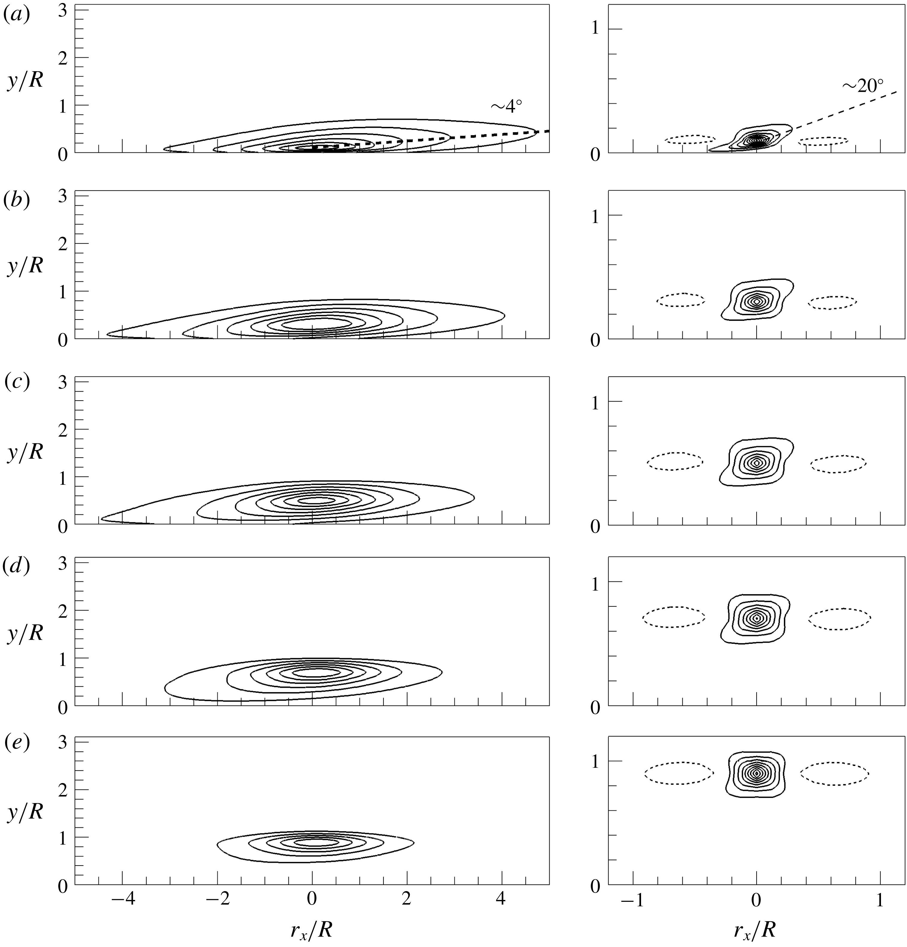Figure 9 shows 2-D contours of the correlations of the VLSM ( $R_{vl}$ ) and LSM ( $R_{l}$ ) in the streamwise-radial plane. The contours of $R_{vl}$ clearly indicate a structure that is asymmetric in the streamwise direction and tilted at a small angle ${\sim}4^{\circ }$ with respect to the wall. This behaviour is contra-indicative of long, streamwise homogeneous roll-cell structures, which would have no asymmetry and no tilt (Baltzer et al. Reference Baltzer, Adrian and Wu2013). Except at $y_{ref}/R=0.1$ , where the correlation is weighted to the downstream, the structures of the VLSM in the outer layer ( $0.3\leqslant y_{ref}/R\leqslant 0.9$ ) reside primarily upstream of the reference point. This effect and the foregoing tilt and asymmetry are consistent with the shape of the low-momentum zone within a single hairpin packet, except that the inclination of the centroid of the low-momentum zone of single packet correlations is expected to be larger. These observations, combined with the length of the correlation concept, are consistent with concatenated hairpin packets. Compared to the VLSM correlations, the LSM correlations (figure 9) in the outer layer contain elements in the lower level contours that indicate structural inclination at clearly larger angles. At $y_{ref}/R=0.1$ , the $15^{\circ }$ – $20^{\circ }$ angle is consistent with established values for the envelope of hairpin packets in the logarithmic layer, but further up the angle steepens to approximately $45^{\circ }$ , consistent with inclination angle of individual hairpins within packets. The streamwise extent of the LSM correlations shows little or no bias fore or aft, suggesting that the effect of differential convection due to mean shear is small.

Figure 9.

Correlation coefficient $R_{vl}$ (lef-hand side) and $R_{l}$ (right-hand side) in the $r_{x}$ – $y$ plane. (a)  $y_{ref}/R=0.1$ , (b) $y_{ref}/R=0.3$ , (c) $y_{ref}/R=0.5$ , (d) $y_{ref}/R=0.7$ , (e) $y_{ref}/R=0.9$ . In $R_{vl}$ , contour levels are varied from 0.05 to 0.3 with an interval of 0.05, and in $R_{l}$ , contour levels are varied from 0.05 to 0.45 with interval of 0.05. A negative contour level of $-0.05$ is included in $R_{vl}$ and $R_{l}$ (dashed line). The mean inclination angles based on a contour level of $R=0.05$ are shown.

Figure 10.

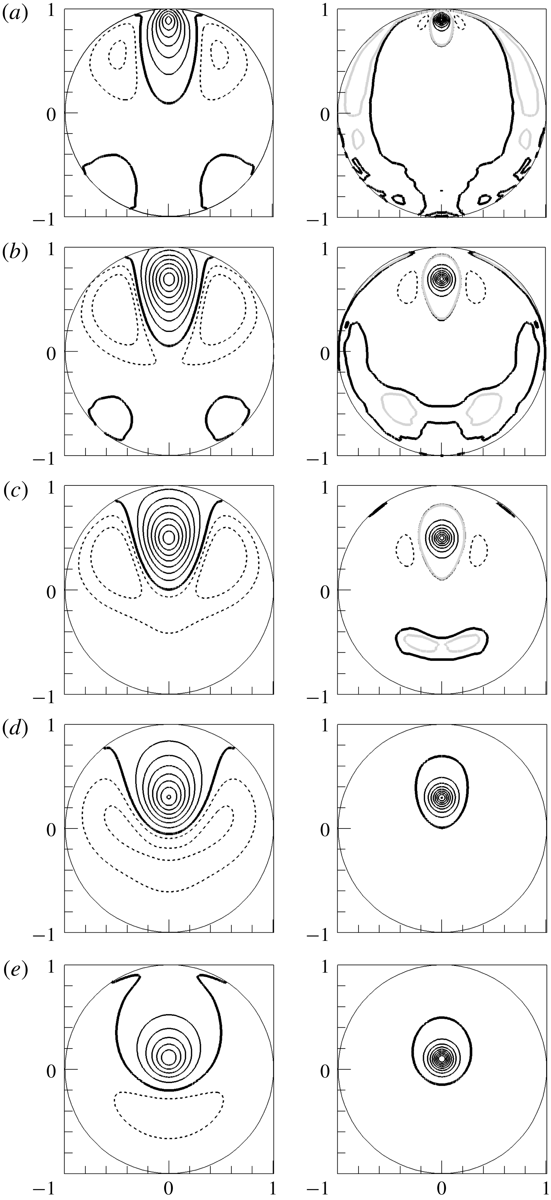
Correlation coefficient $R_{vl}$ (left-hand side) and $R_{l}$ (right-hand side) in the cross-stream plane. (a) $y_{ref}/R=0.1$ , (b) $y_{ref}/R=0.3$ , (c) $y_{ref}/R=0.5$ , (d) $y_{ref}/R=0.7$ , (e)  $y_{ref}/R=0.9$ . Contour levels are varied from 0 to 0.4 with an interval of 0.05 including $-0.025$ and $-0.05$ . The bold black solid line indicates the 0-contour level and dashed lines indicate negative values, respectively. For $R_{l}$ in (a–c), the correlation contour of 0.0005 is depicted with a bold grey solid line.

The correlation functions of the streamwise velocity of VLSM and LSM are examined on the cross-stream plane in figure 10. The bold zero contours separate regions of positive and negative correlation. Positive correlations of the VLSM are flanked by regions of negative correlation, indicating long, low-momentum zones flanked by high momentum zones, or vice versa. The positive regions extend to the near-wall layer, even for reference heights up to $y_{ref}/R=0.9$ , showing clearly the influence of the footprints of the VLSMs on the near-wall region (Mathis et al. Reference Mathis, Hutchins and Marusic2009). Two secondary regions of weak, positive VLSM correlation occur at ${\sim}140^{\circ }$ and ${\sim}220^{\circ }$ from the event location at $0^{\circ }$ for reference points lying below $y_{ref}/R=0.5$ . They, too, penetrate the near-wall region. Baltzer et al. (Reference Baltzer, Adrian and Wu2013) observed similar patterns of weak, positively correlated streaks in $R_{uu}$ up to approximately $y_{ref}/R=0.4$ .

The 0-contour $R_{l}$ (right-hand side of figure 10) fails to convincingly reveal secondary regions of positive correlation, but the grey contour level on which $R_{l}=0$ .0005 does show secondary regions of positive correlation, especially at $y_{ref}/R=0.3$ and 0.5. Unlike the secondary positive correlation regions of the VLSMs, those of the LSMs depend strongly on the wall-normal location of the reference points, separating from the wall with increasing $y_{ref}/R$ and disappearing above $y_{ref}/R=0.7$ . The LSMs separate in the sense that the regions of positive correlation at $r_{x}/R=0$ in $R_{l}$ do not reach the wall at $y_{ref}/R\geqslant 0.1$ . However, the 2-D contour of $R_{l}$ in the $r_{x}$ –y plane in the logarithmic layer (figure 8) is attached to the wall at an upstream location. The contribution of the attached hairpin vortex to the generation of the correlation patterns in the logarithmic layer is consistent with Townsend’s attached eddy hypothesis in which geometrically self-similar attached eddies occur in a hierarchy of scales with a population density of eddies that varies inversely with size and thus with distance from the wall (Townsend Reference Townsend1976; Marusic & Monty Reference Marusic and Monty2019). However, the less streamwise coherence of the correlation contours above the logarithmic layer (figure 9) implies that detached eddies, which may be formed locally away from the wall or are physically detached due to a saturation of the self-similar growth of hairpins attached to the wall, play a dominant role to generation of the correlation patterns.

Bailey & Smits (Reference Bailey and Smits2010) reported that the azimuthal scales of the LSMs in the wake region (termed ‘detached LSMs’) and the VLSMs in the logarithmic layer are approximately the same, leading them to suggest that, and if the hypothesis of Kim & Adrian (Reference Kim and Adrian1999) is valid, then only the larger, older, detached LSMs in the outer layer rather than the smaller hairpin packets located near the wall align to create VLSMs. In figure 10, we find the same approximate equality of azimuthal length scales of the VLSM in the logarithmic layer and the LSM in the outer layer ( $y_{ref}/R>0.5$ ), despite the wavenumber separating VLSM and LSM differing from that of Bailey & Smits (Reference Bailey and Smits2010). Based on the observations of LSMs in the outermost edge of the boundary layer (Kovasznay et al. Reference Kovasznay, Kibens and Blackwelder1970; Falco Reference Falco1977), Kim & Adrian (Reference Kim and Adrian1999) and succeeding publications from that group have consistently defined LSMs in pipes and channels to be 2– $3R$ long structures whose wall-normal extent approaches the centreline. They have further interpreted the LSMs to be the oldest and therefore largest packets. Since the largest packets contain smaller packets in a hierarchy of scales (Adrian et al. Reference Adrian, Meinhart and Tomkins2000), the attached smaller packets in the near-wall region with strong streamwise fluctuating velocity contribute to align the adjacent packets. Note that in figure 4, the tallest detached packet was shown to overrun the near-wall attached packet to form the VLSM. This scenario suggests that the LSMs and VLSMs are interrelated.

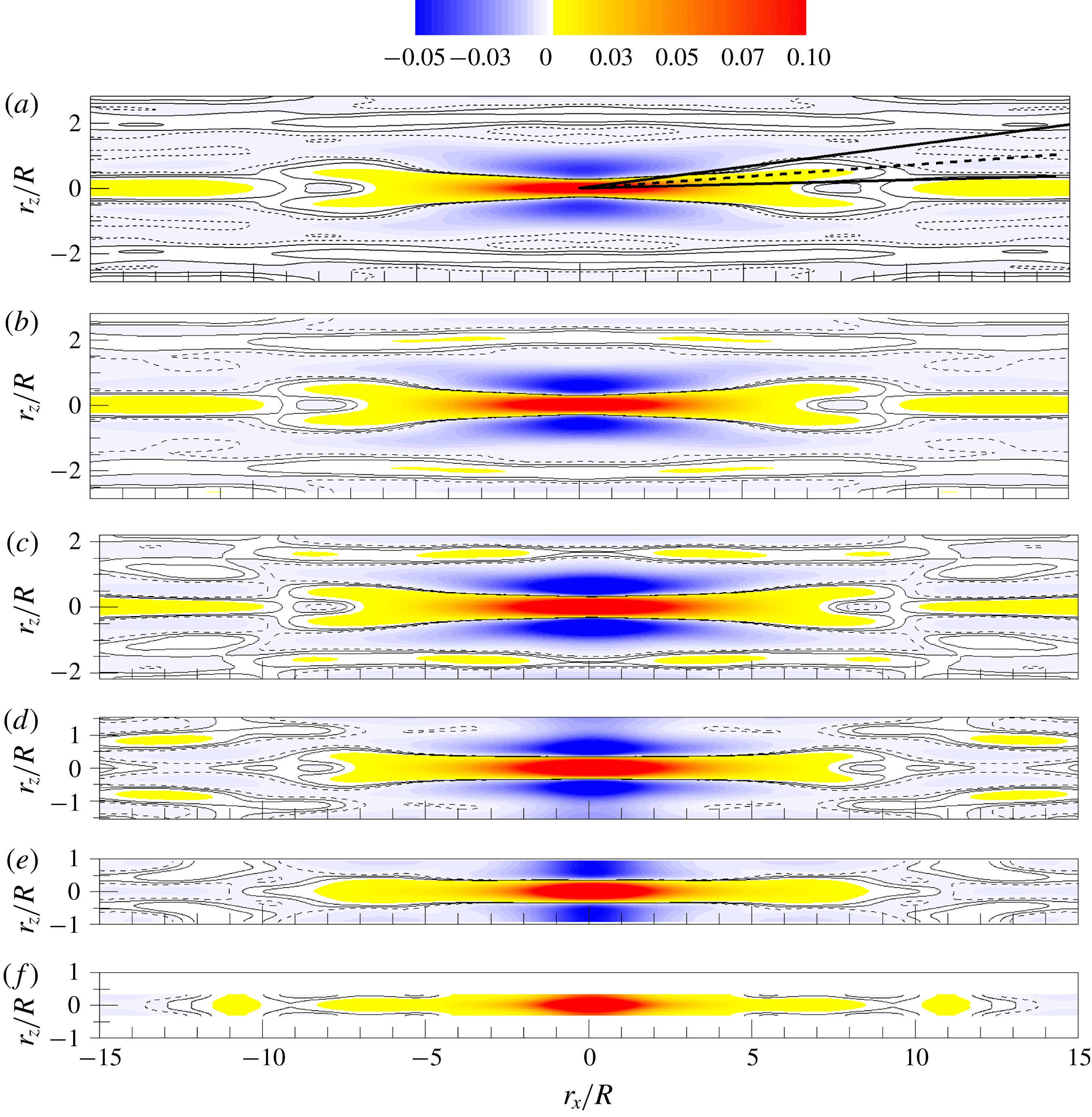
Figures 11 and 12 display correlation coefficients $R_{vl}$ and $R_{l}$ in the $r_{x}{-}r_{z}$ plane using low values to expose the LSM and VLSM patterns (large correlation coefficients occur at small separation by virtue of the small-scale contributions; to see the large scales, one must accept the low correlation coefficients that occur at large separations). Correlation on the plane $y_{ref}/R=0.15$ is included for future reference. The contour levels range from $-0.05$ to 0.1, with solid and dashed lines corresponding to contour levels of 0, 0.001 and $-0.001$ . Below $y_{ref}/R=0.5$ the contours of $R_{vl}$ exhibit X-shaped patterns at very-large-scale separations between $5R$ and $10R$ (the regions in yellow). We will see that the X is a superposition of positively and negatively inclined alignments of LSMs along shallow ( ${\sim}5^{\circ }$ – $10^{\circ }$ ) helical angles. The helical angle of the VLSM and the LSM is defined as the mean of the largest and smallest helical angles, as shown in figures 11(a) and 12(a). 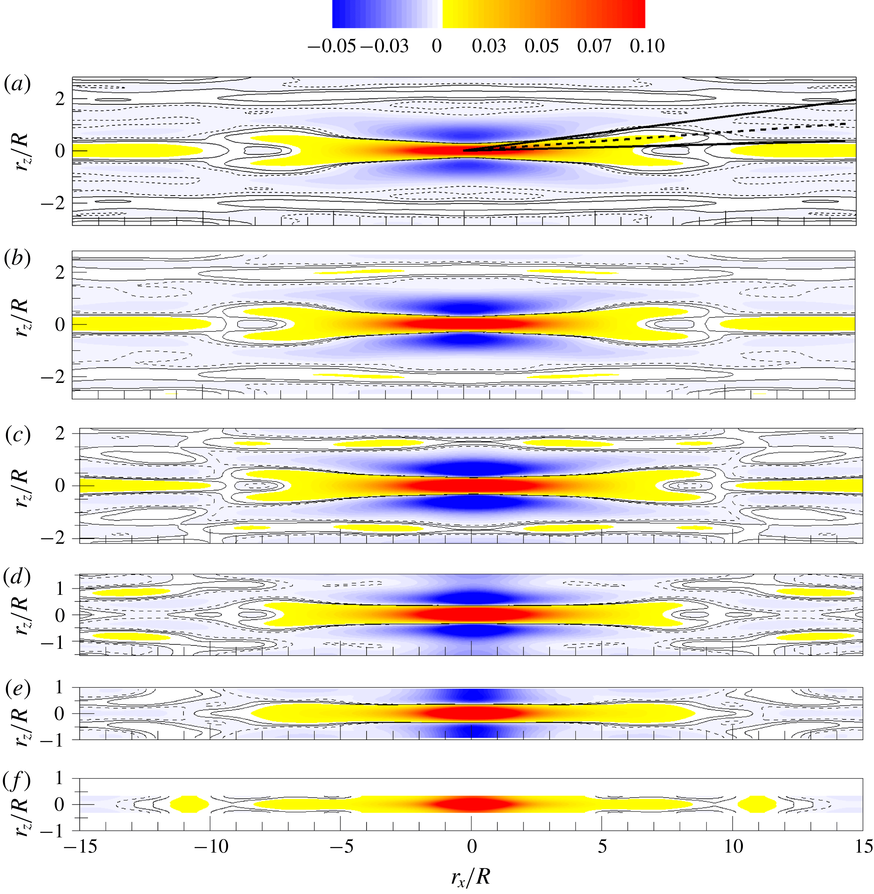At separations less than $5R$ the X-shape merges into a red region of high correlation flanked by spanwise-offset regions of negative (blue) then positive (pale yellow) correlation. In the streamwise direction the correlation briefly turns negative at approximately 8- $9R$ , then resumes a positive value. As noted in Baltzer et al. (Reference Baltzer, Adrian and Wu2013) the presence of the features at these low contour levels is due neither to noise, nor lack of statistical convergence, nor streamwise periodicity of the simulation, because previous experimental studies reported similar behaviour. The X-shape correlation pattern has also been reported in a boundary layer study using Taylor’s hypothesis (Hutchins & Marusic Reference Hutchins and Marusic2007a ). They also showed that an X-shape could be produced by correlating three adjacent, $12R$ -long strips of high–low–high speed flow that meandered sinusoidally in the spanwise direction. The single frequency meandering created periodic regions of positive and negative correlation in the streamwise direction with a period of $3.5R$ . The similar positive region in our pipe flow simulation is more elongated ( $r_{x}\sim 7R$ ) in figure 11 with additional regions of positive correlation offset in the streamwise and spanwise directions. However, it is hard to make such a pattern using a simple meandering low-speed streak. Later, we will show that the superposition of helically inclined VLSM modes, similar to those observed in the instantaneous fields, can induce complex spatial organization similar to that found in figure 11.

Figure 11.

Correlation coefficient $R_{vl}$ in the $r_{x}{-}r_{z}$ plane. (a) $y_{ref}/R=0.1$ , (b) $y_{ref}/R=0.15$ , (c) $y_{ref}/R=0.3$ , (d) $y_{ref}/R=0.5$ , (e) $y_{ref}/R=0.7$ , (f) $y_{ref}/R=0.9$ . Colour contour levels are varied from $-0.05$ to 0.1, and solid lines depict the low contour levels of the correlations, corresponding to 0, 0.001 and $-0.001$ (dashed line). Thick, straight solid lines in (a) indicate the largest and smallest helical angles for the VLSM, and thick, straight dashed lines depict the mean helical angle.

Figure 12.

The same as figure 11, but for correlation coefficient $R_{l}$ in the $r_{x}{-}r_{z}$ plane. In (a), the enlarged view of a region in the vicinity of the reference location is included in the right-hand corner for clarity.

In figure 12, the correlation pattern of the LSM, $R_{l}$ , also exhibits an X-pattern, but the angle of inclination is much larger than the helical angles found for the VLSM, and the streamwise and spanwise scales are, of course, smaller. The small region of positive correlation is surrounded fore-and-aft and side-to-side by regions of negative correlation. Although the region of positive correlation is surprisingly small, this pattern is consistent with the correlation of a single hairpin packet, but the X-pattern is not.

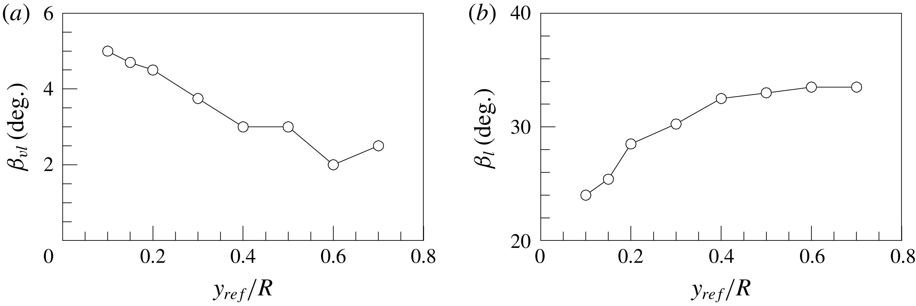
We now examine the variation of the correlation-based helical angles for the VLSM and the LSM along the wall-normal direction. Figures 11 and 12 make it clear that the helical angle depends on the value of the threshold employed. Since low contour levels of both VLSMs and LSMs create an X-shape pattern, we have chosen $R=0.0005$ as a representative low contour level to measure the helical angles of the structures with opposite sign. In figure 13(a), the dominant helical angle of the VLSM ( $\unicode[STIX]{x1D6FD}_{vl}$ ) is shown to decrease continuously with increasing $y/R$ , probably due to the decrease of the azimuthal domain (figure 11), creating less helical angle. Contrary to the observation for the VLSMs, the highly tilted helical angle of the LSM ( $\unicode[STIX]{x1D6FD}_{l}$ ) increases continuously in the outer layer (figure 13 b). As shown in figure 12, the increase of the helical angle of the LSM seems to be due to high growth rate of the spanwise length scale of the LSMs than that of the streamwise length scale with the distance from the wall.

Figure 13.

Azimuthally offset angle variations of the (a) VLSMs and (b) LSMs based on $R=0.005$ .

5 Reconstruction of $R_{vl}$ and $R_{l}$

In this section, we will provide evidence that the spatial organization pattern of $R_{vl}$ discussed in the previous section can be constructed by a combination of several helically aligned VLSM patterns based on energetic POD modes. The identified VLSM patterns that are created by artificial packets of hairpin vortices can reconstruct both $R_{vl}$ and $R_{l}$ based on spectral filtration of the signal.

5.1 Proper orthogonal decomposition analysis

We first consider the Karhunen–Loeve procedure to extract the most energetic coherent structures (POD modes) from the eigenfunctions of the two-point correlation tensor in the Fourier domain (Duggleby et al. Reference Duggleby, Ball, Paul and Fischer2007; Baltzer Reference Baltzer2012)

(5.1) $$\begin{eqnarray}\int _{0}^{R}\unicode[STIX]{x1D61A}_{ij}(k_{x},r,k_{\unicode[STIX]{x1D703}};r_{ref})\hat{\unicode[STIX]{x1D6F9}}_{j}^{(n)}(k_{x},r,k_{\unicode[STIX]{x1D703}})r\,\text{d}r=\unicode[STIX]{x1D706}^{(n)}(k_{x},k_{\unicode[STIX]{x1D703}})\hat{\unicode[STIX]{x1D6F9}}_{i}^{(n)}(k_{x},r_{ref},k_{\unicode[STIX]{x1D703}}),\end{eqnarray}$$

where $\hat{\unicode[STIX]{x1D6F9}}$ is the Fourier-transformed eigenfunction with associated eigenvalue $\unicode[STIX]{x1D706}$ , and $n$ is an index assigned to each POD mode by ordering according to decreasing energy. The spectral-density tensor $\unicode[STIX]{x1D61A}_{ij}$ is calculated from discrete Fourier-transformed velocity $\hat{u} _{i}(k_{x},r,k_{\unicode[STIX]{x1D703}})$ as

(5.2) $$\begin{eqnarray}\unicode[STIX]{x1D61A}_{ij}(k_{x},r,k_{\unicode[STIX]{x1D703}};r_{ref})=\langle u_{i}(k_{x},r_{ref},k_{\unicode[STIX]{x1D703}})u_{j}^{\ast }(k_{x},r,k_{\unicode[STIX]{x1D703}})\rangle ,\end{eqnarray}$$

where (*) denotes the complex conjugate of the eigenfunction. Due to the homogeneity and periodicity in $x$ and $\unicode[STIX]{x1D703}$ each velocity component of the POD modes varies trigonometrically as a function of the $x$ and $\unicode[STIX]{x1D703}$ spatial coordinates, i.e. the modes are Fourier in those directions. Each mode is assigned a mode number set $(i_{x},i_{\unicode[STIX]{x1D703}},n)$ , where $i_{x}$ and $i_{\unicode[STIX]{x1D703}}$ are indices for which the corresponding mode wavenumbers are

(5.3a,b ) $$\begin{eqnarray}k_{x}=\frac{2\unicode[STIX]{x03C0}}{30R}i_{x}\quad \text{and}\quad k_{\unicode[STIX]{x1D703}}=i_{\unicode[STIX]{x1D703}}.\end{eqnarray}$$

In the latter, we will use both notions, ( $i_{x}$ , $i_{\unicode[STIX]{x1D703}}$ ) and ( $k_{x}$ , $k_{\unicode[STIX]{x1D703}}$ ), as convenient. Since the eigenvalue indicates the mean amounts of turbulent kinetic energy that each POD mode contributes to reconstructed fields, the most energetic modes with $n=1$ are particularly important in organizing the flow. The $n=1$ eigenvalues for each streamwise and azimuthal wavenumber index in table 1 include the sum of all Fourier modes with positive and negative wavenumber values for the indices. The 10 most dominant modes are depicted in bold. The $n=1$ modes account for approximately 90 % of total kinetic energy for all ( $i_{x}$ , $i_{\unicode[STIX]{x1D703}}$ ) pairs, and the most energetic modes are observed in VLSM wavelengths, consistent with a previous study of Baltzer et al. (Reference Baltzer, Adrian and Wu2013).

Table 1.

Eigenvalue spectrum of the $n=1$ POD modes for the unfiltered pipe flow (e.g. using $R_{uu}$ in the POD kernel). The eigenvalues in bold correspond to the 10 most energetic Fourier modes. The superscript 1 indicates mode combination 1.

The orthogonal eigenfunctions obtained from (5.1) can be used to reconstruct the two-point spatial correlation tensor with the corresponding eigenvalues. The two-point spatial correlation tensor is given by Baltzer (Reference Baltzer2012) and Holmes et al. (Reference Holmes, Lumley, Berkooz and Rowley2012)

(5.4) $$\begin{eqnarray}R_{ij}(r_{x},r,r_{\unicode[STIX]{x1D703}};r_{ref})=\mathop{\sum }_{k_{x}}\mathop{\sum }_{k_{\unicode[STIX]{x1D703}}}\mathop{\sum }_{n}\unicode[STIX]{x1D706}^{(n)}(k_{x},k_{\unicode[STIX]{x1D703}})\hat{\unicode[STIX]{x1D6F9}}_{i}^{(n)}(k_{x},r_{ref},k_{\unicode[STIX]{x1D703}})\hat{\unicode[STIX]{x1D6F9}}_{j}^{(n)\ast }(k_{x},r,k_{\unicode[STIX]{x1D703}})\text{e}^{\,j(k_{x}r_{x}+k_{\unicode[STIX]{x1D703}}r_{\unicode[STIX]{x1D703}})}.\end{eqnarray}$$

This equation (5.4) indicates that $R_{ij}$ can be decomposed into the sum of the weighted (by $\unicode[STIX]{x1D706}$ ) two-point correlation tensors of the eigenfunctions for all ( $i_{x}$ , $i_{\unicode[STIX]{x1D703}}$ , $n$ ) triples, and inverse Fourier transform back into physical space. Since the $n=1$ modes contribute most significantly to the flow, we focus on the structures of the $n=1$ mode. Furthermore, since the dominant X-shaped pattern in $R_{vl}$ consists of wavelengths larger than $15R$ in figure 11, we shall focus on Fourier modes $i_{x}=0$ , 1, 2; as an example, five energetic modes $(i_{x},i_{\unicode[STIX]{x1D703}},n)=(2,\pm 3,1),(0,\pm 2,1)$ , ( $0,\pm 3,1$ ), ( $1,\pm 1,1$ ) and ( $2,\pm 4,1$ ) with VLSM modes $i_{x}=0$ , 1, 2. The modes are energy ordered in table 1, with $n=1$ being the most energetic mode. Their linear sum, properly weighted by $\unicode[STIX]{x1D706}^{(n)}(k_{x},k_{\unicode[STIX]{x1D703}})$ , is able to reproduce an X-shaped correlation pattern of $R_{vl}$ , similar to that in figure 11(b) in the logarithmic layer. The components of the 4th, 6th, 7th, 8th and 9th energetic modes are grouped as mode combination 1 in table 1. These five modes are among the longest VLSM wavelengths more than $15R$ long, and the helical angles of the modes ( $\unicode[STIX]{x1D6FD}_{vl}$ ) vary from $0^{\circ }$ to $10.1^{\circ }$ by the relation $\unicode[STIX]{x1D6FD}_{vl}=\tan ^{-1}[(R-y)2\unicode[STIX]{x03C0}i_{x}/(L_{x}i_{\unicode[STIX]{x1D703}})]$ at a particular $y$ location with a wavenumber pair ( $i_{x}$ , $i_{\unicode[STIX]{x1D703}}$ ) (Baltzer et al. Reference Baltzer, Adrian and Wu2013). The helical angle of $\unicode[STIX]{x1D6FD}_{vl}\sim 5.0^{\circ }$ at $y_{ref}/R=0.1$ indicates a mode relation $i_{x}\sim 0.464i_{\unicode[STIX]{x1D703}}$ , implying that the helical angle at this height is not simply obtained from a single dominant VLSM pattern, consistent with our previous observation in figures 10 and 11 with the secondary peak of the positive-offset regions closer to $140^{\circ }$ and $220^{\circ }$ . Although not shown here, another mode combination of eigenmodes can be made for $R_{vl}$ with clear X-shape pattern, for instance using 4th, 7th, 8th and 9th energetic modes or 2nd, 4th, 7th, 8th, 12th, 14th, 16th and 18th energetic modes and so on. However, simply summing the five (or more) most energetic modes only provides a highly elongated correlation pattern in the streamwise direction without the X-shaped contour.

Figure 14.

Correlation coefficient $R_{vl}$ at $y_{ref}/R=0.15$ in the $r_{x}$ – $r_{z}$ plane with (a) $R_{vl}$ based on present DNS data and (b) $R_{vl}$ based on superposition of the five energetic eigenmodes. Contour levels are varied from $-0.05$ to 0.1, and the solid lines depict the 0-contour level. Thick, straight dashed lines depict the mean helical angle ${\sim}4.5^{\circ }$ .

The streamwise-elongated pattern with no X-shape pattern and high energy is consistent with results by snapshot POD method that is based on no scale decomposition in $x$ - and $\unicode[STIX]{x1D703}$ -directions to calculate POD modes (Hellström, Sinha & Smits Reference Hellström, Sinha and Smits2011). In turbulent pipe flow at $\mathit{Re}_{D}=12\,500$ , they found that the most energetic POD mode ( $n=1$ ) that is the sum of all ( $i_{x}$ , $i_{\unicode[STIX]{x1D703}}$ ) pairs consists of straight, streamwise-aligned segments of positive and negative streamwise velocity fluctuating structures. They also noted that the superposition of the four most energetic modes ( $n=1{-}4$ ) will recreate meandering structures, indicating that the alignment of spanwise-offset small scales of motions creates the appearance of VLSM.

Figure 14 shows correlation coefficients $R_{vl}$ calculated from the present DNS data and from the superimposition of the above five energetic modes (mode combination 1) with positive and negative azimuthal wavenumber pair at $y_{ref}/R=0.15$ (highest extent of logarithmic layer) in which VLSMs are frequently observed to be populated. The dominant X-shape pattern of the correlation with highly elongated positive region ( ${\sim}7R$ long) shown in figure 14(a) is clearly apparent in the reconstructed $R_{vl}$ . The mean helical angle of $\unicode[STIX]{x1D6FD}_{vl}\sim 4.5^{\circ }$ (thick, bold dashed lines) averaged with the five energetic modes is in good agreement with the real one. In addition, positively correlated regions with the streamwise- and spanwise-offsets found in figures 10 and 11 are obviously shown with non-periodic spacing in $x$ and $\unicode[STIX]{x1D703}$ , although the location of secondary positive maxima with the spanwise-offset in figure 14(b) is slightly closer to the reference location at $r_{x}/R=0$ . The difference of the contour levels between figures 14(a) and 14(b) is due to neglecting the other modes, and this indicates that other VLSM structures with different helical angles and wavelengths are also important in constructing the full structural organization pattern of the true correlation $R_{vl}$ . The similarity of the reconstructed $R_{vl}$ to the real one demonstrates that the complex X-shaped correlation pattern of $R_{vl}$ (or low contour level of $R_{uu}$ ) with the offset regions in the streamwise and spanwise directions is not simply due to a dominant outer layer large-scale structure (e.g. very long meandering motion). It also requires the superposition of helically inclined very long structures (4th, 8th and 9th modes) and streamwise-aligned motions (6th and 7th modes).

Figure 15 displays vector patterns of reconstructed $v$ and w modes with isosurfaces of reconstructed $u$ mode for the five dominant POD modes of mode combination 1. The vortices and associated large-scale patterns in the POD modes are periodically arranged along the pipe’s circumference, and the modes take helical form encompassing all radii with rotation as $x$ varies, unless $i_{x}$ is non-zero. Here, we visualize counterclockwise modes. A similar set of clockwise modes also exists for oppositely signed azimuthal wavenumber. The most dominant patterns in figure 15 are those of roll-cells, indicating a close association with VLSMs. The strength of the roll-cell modes is maximum for $(i_{x},i_{\unicode[STIX]{x1D703}})=(2,4)$ , indicating that the strength of the roll-cells is proportional to the number of azimuthal wavenumber. In addition, the roll-cells clearly influence near-wall structures regardless of the POD mode pair, based on observations that the roll-cells are centred far from the wall at $y/R=0.29{-}0.41$ , and the roll-cells’ influences are strong in the near-wall region, consistent with the interaction between inner and outer layers (Mathis et al. Reference Mathis, Hutchins and Marusic2009). Although not shown here, linear estimates of conditional averages with a $-u$ event at $y_{ref}/R=0.15$ using the VLSM correlation on the cross-stream plane exhibit large-scale counter-rotating roll-cells with strong eruptions and sweep motions, consistent with the reconstructed POD modes in figure 15 (blue colour). This indicates that the large roll-cells could sweep near-wall hairpin packets into alignment along the stagnation zones between cells (Toh & Itano Reference Toh and Itano2005; Adrian Reference Adrian2007). However, it is not clear whether the roll-cell also nudges the LSMs into alignment, or the LSM alignment creates the roll-cells.

Figure 15.

Roll-cell-like behaviour of the five POD modes with (a) ( $i_{x}=2$ , $i_{\unicode[STIX]{x1D703}}=3$ ), (b) ( $i_{x}=0$ , $i_{\unicode[STIX]{x1D703}}=2$ ), (c) ( $i_{x}=0$ , $i_{\unicode[STIX]{x1D703}}=3$ ), (d) ( $i_{x}=1$ , $i_{\unicode[STIX]{x1D703}}=1$ ) and (e) ( $i_{x}=2$ , $i_{\unicode[STIX]{x1D703}}=4$ ). The left-hand side plots display the colour contours of reconstructed $u$ with in-plane velocity vectors of $v$ and $w$ modes at $x/R=0$ planes, and the right-hand side red and blue isosurfaces indicate the swirling patterns of positive and negative $u$ -structures (at one-half of maximum and minimum).

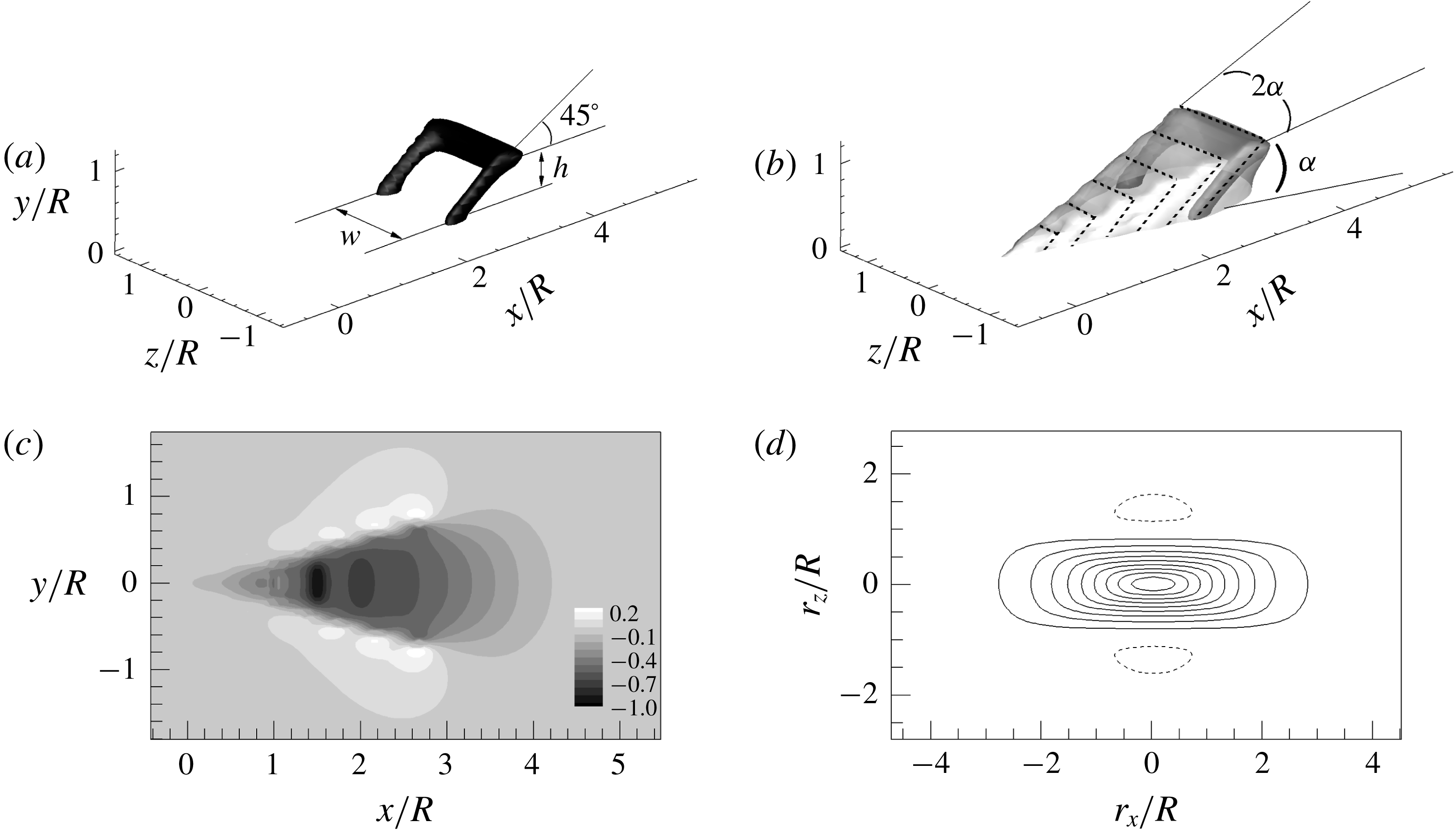
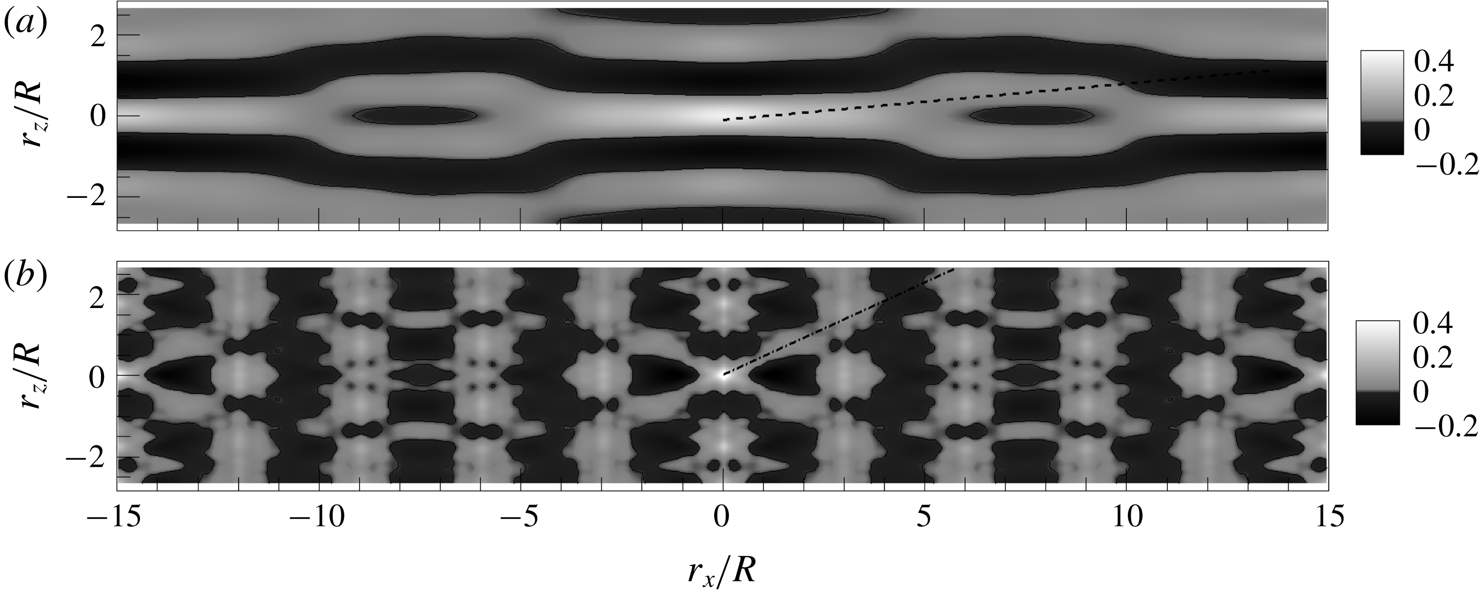
5.2 Hairpin packet model

To provide clear evidence for how spatial organization patterns of both $R_{vl}$ and $R_{l}$ are created in the flow field based on the model of VLSMs, we consider a hairpin model devised from the work of Perry & Chong (Reference Perry and Chong1982) and Perry & Marusic (Reference Perry and Marusic1995). In their model, a hairpin has the shape of a goalpost inclined at $45^{\circ }$ to the wall in the downstream direction. The induced velocity created by the model is calculated based on the Biot–Savart law.

Figure 16(a) shows the typical structure of a hairpin vortex represented by an isosurface of negative streamwise velocity. Here, the contour level is chosen to clearly show the hairpin-like structure with 20 % of minimum (negative maximum). The legs (or neck) of the goalpost-like hairpin are attached to the wall, and the inclination angle of the structure is maintained to be constant with $45^{\circ }$ for simplicity. The packet in figure 16(b) consists of six hairpin vortices that are streamwise-aligned with spacing $0.5R$ . The height ( $h$ ) of the hairpins varies linearly from $0.1R$ to $0.7R$ with an interval of $0.12R$ , creating a packet growing upwards in the streamwise direction at a mean angle of approximately $\unicode[STIX]{x1D6FC}=13.5^{\circ }$ (Zhou et al. Reference Zhou, Adrian, Balachandar and Kendall1999; Adrian et al. Reference Adrian, Meinhart and Tomkins2000). Note that the width of the hairpins is taken to be twice that of the hairpin height based on the data of Tomkins & Adrian (Reference Tomkins and Adrian2003). The induced velocity within and around a packet is simply the linear summation of the velocities induced by individual hairpin vortex. The induced velocity and correlation patterns by a packet in figure 16(c,d) are similar to those found in the literature (Zhou et al. Reference Zhou, Adrian, Balachandar and Kendall1999; Tomkins & Adrian Reference Tomkins and Adrian2003).

Figure 16.

(a) Goalpost-like model of a single hairpin vortex (Perry & Marusic Reference Perry and Marusic1995). The hairpin is inclined to the flow direction with $45^{\circ }$ . (b) Hairpin packet model (grey colour) constructed here using 6 hairpins (dashed lines). The height ( $h$ ) of the hairpins is varied linearly from $0.1R$ to $0.7R$ and the width ( $w$ ) is $2h$ . The growth angle is constant, $\unicode[STIX]{x1D6FC}=13.5^{\circ }$ . The individual hairpins in (b) are separated with spacing of $\unicode[STIX]{x1D6FF}x/R=0.5$ in the streamwise direction, creating a $3R$ -long hairpin packet, enveloping an LSM. The hairpin in (a) is the 6th hairpin in the packet, as shown in (b) with transparent view. The isosurface contours in (a) and (b) are the negative streamwise velocity. (c) The $u$ velocity induced inside and outside the model packet at $y_{ref}/R=0.15$ (normalized by the negative maximum) and (d) line contours of the correlation coefficient of the streamwise velocity on the $r_{x}$ – $r_{z}$ plane at $y_{ref}/R=0.15$ . The contour levels are varied from 0.1 to 0.9, and the dashed line depicts $R=-0.05$ .

Figure 17.

(a) Perspective view of the synthetically constructed pattern ( $u$ velocity with 20 % of minimum) associated with the counterclockwise 4th mode $(i_{x},i_{z})=(2,3)$ . The top view of the pattern is shown in the right-hand corner, and the flow direction is from left to right. Spatial two-point correlations using the pattern in (a) where (b) $R_{uu}$ , (c) $R_{vl}$ and (d) $R_{l}$ . The high- and low-pass filters in figure 7 were employed, and the reference wall-normal height is $y_{ref}/R=0.15$ . The dominant helical angles for VLSM ( $\unicode[STIX]{x1D6FD}_{vl}$ ) and LSM ( $\unicode[STIX]{x1D6FD}_{l}$ ) are defined in (c) and (d) with dashed and dashed-dot lines. Here $\unicode[STIX]{x1D6FD}_{vl}$ and $\unicode[STIX]{x1D6FD}_{l}$ are ${\sim}6.8^{\circ }$ and ${\sim}25.4^{\circ }$ for the 4th mode. In addition, the relevant LSM patterns for $\unicode[STIX]{x1D6FD}_{vl}$ and $\unicode[STIX]{x1D6FD}_{l}$ are described in (a) with dashed and dashed-dot lines.

We construct the five energetic VLSM modes described in § 5.1 by aligning the above artificially generated hairpin packets along helical angles (with spanwise-offset) that are very consistent with those of the five modes in figure 15. An example of an artificially constructed VLSM pattern corresponding to the counterclockwise 4th mode $(i_{x},i_{z})=(2,3)$ is shown in figure 17(a) with its correlation patterns (b) $R_{uu}$ , (c) $R_{vl}$ and (d) $R_{l}$ using the high- and the low-pass filters employed in figure 7. Here, the computational domain is $(L_{x},L_{y},L_{z})=(30R,1.25R,2\unicode[STIX]{x03C0}\ast 0.85R)$ to be consistent with the domain size in the logarithmic layer in figures 14 and 15. The configuration in figure 17 is clearly shown when the cylinder in figure 15(a) is rolled out to be viewed as a plane at $y/R=0.15$ . In addition, figure 18 shows correlation patterns using both positive and negative spanwise wavenumber pair for the 4th mode, i.e. clockwise and counter-clockwise helices, compared to that in figure 17. Since the hairpin packets are continuously aligned along the helical alignment related to the 4th POD mode both with spanwise-offset and with a streamwise-interval similar to that between the hairpins, there exist 10 hairpin packets along the helical lines over the $30R$ long domain. As expected, the correlation $R_{vl}$ with low contour level of $R_{uu}$ in figure 17 shows that the highly elongated positive VLSM pattern is flanked by negatively correlated regions on each side due to vortex induction from the legs and the head, and the correlation is inclined at a helical angle due to spanwise-inclined VLSMs related to the 4th mode. In addition, the correlations of $R_{uu}$ and $R_{vl}$ seem to contain meandering behaviour along the helically inclined VLSM alignment (see the top view in figure 17 a), and it is more pronounced in $R_{uu}$ rather than $R_{vl}$ due to the smoothing effect of the VLSM filter. This demonstrates that the meandering is possibly due to spanwise-offset LSMs that are relatively straight, not due to a dominant meandering motion residing in turbulent flow. The meandering behaviour based on our result is consistent with the previous observations of Balakumar & Adrian (Reference Balakumar and Adrian2007) that ‘the smoothed field of a concatenation of misaligned hairpin packets would look like a pair of meandering counter-rotating streamwise vortices’. Furthermore, our result is consistent with the study of Hellström et al. (Reference Hellström, Sinha and Smits2011) based on snapshot POD modes in which they showed that reconstructions with the 10 most energetic POD modes ( $n=1{-}10$ ) capture all the principal characteristics of the VLSM, suggesting that VLSMs are constructed of the most energetic POD modes that give the impression of long meandering structures.

Figure 18.

Spatial two-point correlations (a) $R_{uu}$ , (b) $R_{vl}$ and (c) $R_{l}$ at $y_{ref}/R=0.15$ using the artificial pattern in figure 17, but using both positive and negative spanwise wavenumber pair. The dominant helical angles for VLSM ( $\unicode[STIX]{x1D6FD}_{vl}$ ) and LSM ( $\unicode[STIX]{x1D6FD}_{l}$ ) present in figure 17 are shown in the figure.

However, the correlation pattern of $R_{l}$ in figure 17(d) shows a clear alternating pattern of positive (white) and negative (black) correlation regions at an angle of $\unicode[STIX]{x1D6FD}_{vl}$ in the streamwise direction. This is attributed to high-momentum regions residing in the upstream of the low-momentum regions due to continuous induction of hairpin vortices, consistent with figure 12. Instead of the long coherent pattern along the angle of $\unicode[STIX]{x1D6FD}_{vl}$ in $R_{l}$ , an elongated pattern of positive correlation region is obviously shown to be created with an inclination angle ( $\unicode[STIX]{x1D6FD}_{l}$ ), as depicted by a white dashed-dot line in figure 17(d). Since we assume that the most upstream packets in each line (along $\unicode[STIX]{x1D6FD}_{vl}$ ) are located in the region of $0\leqslant x/R\leqslant L_{l}$ , then the mode helical angle for the LSM at a particular $y$ location and with a wavenumber pair ( $i_{x}$ , $i_{z}$ ) can be defined by

(5.5) $$\begin{eqnarray}\unicode[STIX]{x1D6FD}_{l}=\tan ^{-1}\left(\frac{(R-y)2\unicode[STIX]{x03C0}}{i_{z}}\left(\frac{1}{L_{l}}-\frac{i_{z}}{L_{x}}\right)\right),\end{eqnarray}$$

where $L_{l}$ is the streamwise length ( $=3R$ ) of each packet. Then, the $(i_{x},i_{z})=(2,3)$ mode has LSM helical angle of $\unicode[STIX]{x1D6FD}_{l}=25.4^{\circ }$ at $y/R=0.15$ in figure 17(d). As can be seen in figure 17(a) with the dashed-dot line, such a positive correlation pattern of $R_{l}$ along with the helical angle $\unicode[STIX]{x1D6FD}_{l}$ is induced by the alignment of LSMs, although each LSM is involved in creating different VLSMs. Inspection of the other four modes with their configurations using the above relation in figure 19 shows helical angles of $\unicode[STIX]{x1D6FD}_{l}=41.7^{\circ }$ ( $i_{x}=0$ , $i_{z}=2$ ), $30.7^{\circ }$ ( $i_{x}=0$ , $i_{z}=3$ ), $57.9^{\circ }$ ( $i_{x}=1$ , $i_{z}=1$ ) and $19.9^{\circ }$ $(i_{x}=2,i_{z}=4)$ with a similar organization pattern to the $(i_{x},i_{z})=(2,3)$ mode, although corresponding correlation patterns (i.e. $R_{uu}$ , $R_{vl}$ and $R_{l}$ ) are not shown here.

Figure 19.

The same as figure 17(a), but for the other four modes. (a) 6th mode $(i_{x},i_{\unicode[STIX]{x1D703}})=(0,2)$ , (b) 7th mode $(i_{x},i_{\unicode[STIX]{x1D703}})=(0,3)$ , (c) 8th mode $(i_{x},i_{\unicode[STIX]{x1D703}})=(1,1)$ and (d) 9th mode $(i_{x},i_{\unicode[STIX]{x1D703}})=(2,4)$ .

Figure 20.

Roll-cell-like behaviour of the artificial five POD modes. Each POD mode is constructed using each artificially constructed VLSM pattern of the five energetic modes with positive and negative spanwise wavenumber pair. (a) $(i_{x},i_{\unicode[STIX]{x1D703}})=(2,\pm 3)$ , (b) (0, $\pm$ 2), (c) (0, $\pm 3$ ), (d) (1, $\pm 1$ ) and (e) (2, $\pm 4$ ). The left-hand plots display the colour contours of $u$ with in-plane velocity vectors of $v$ and $w$ modes at $x/R=0$ planes, and the right-hand white and black isosurfaces indicate the swirling patterns of positive and negative $u$ -structures (at one-half of maximum and minimum).

Although the VLSM mode of $(i_{x},i_{z})=(2,3)$ is one of the most energetic modes in the eigenvalue spectrum and has wide influence in organizing the flow pattern, strong local energy contributions to the total energy are primarily from the sum of LSM and smaller scales of motions, as shown in figure 17(d) with deep white and black contours. The contour coefficients $R_{vl}$ and $R_{l}$ normalized by the mean square value of $u$ in figures 10–12 also show the consistent behaviour to the energy contributions from LSMs and VLSMs. Baltzer et al. (Reference Baltzer, Adrian and Wu2013) analysed an instantaneous field with an energetic mode $(i_{x},i_{z})=(2,3)$ , and they showed that the typical strength of the very long $u$ -structure with the mode is more than 20 times smaller than that of the raw data at $y/R=0.15$ , indicating that the highly energetic VLSMs should be combined with smaller scales of motions contributing to strong local net energy to consist of a total energy for a raw instantaneous realization. The energy relationship is consistent with the hypothesis that the largest scales are composed of concatenations of LSMs.

Figure 20 shows constructed POD modes using the artificially constructed VLSM patterns of the energetic five modes of mode combination 1. Here, each POD mode is calculated using each corresponding VLSM pattern with a positive and negative spanwise wavenumber pair among the five energetic modes, i.e. in figure 20(a), the artificial VLSM pattern, which resembles the pattern corresponding to the 4th mode $(i_{x},i_{z})=(2,\pm 3)$ , is first made by the alignment of the artificial LSMs with positive and negative spanwise wavenumber pair, and the energetic POD mode with wavenumber pair $(i_{x},i_{z})=(2,\pm 3)$ is constructed based on its correlation pattern shown in figure 18(a). This approach results in the most energetic $n=1$ POD mode at the $(i_{x},i_{z})=(2,3)$ wavenumber pair in figure 20(a), corresponding to the wavenumber pair related to the 4th energetic mode (figure 15 a).

In figure 20, the very-large-scale counter-rotating roll-cell-like vortex patterns are periodically organized in the streamwise and spanwise directions except for the rotation when varying the streamwise location for non-zero $i_{x}$ . The roll-cells for the modes are centred at $y/R=0.28$ , 0.34, 0.3, 0.37 and 0.2, and the trend of the position is comparable to $y/R=0.33$ , 0.38, 0.34, 0.41 and 0.29 in figure 15 for the real ones, although there are small discrepancies in magnitude. The roll-cell motions are present for either the streamwise-aligned or spanwise-inclined VLSM pattern, and the general shape of the contours for all the roll-cells is relatively insensitive to the number of roll-cell pairs, consistent with those in figure 15. This indicates that the artificial packet alignments for the VLSMs replicate the topology of the modal flow pattern for each five mode. However, some differences are clearly observed in particular in the near-wall region. That is, the isosurfaces of the roll-cells in the 3-D view in figure 20 are not closed in the near-wall region. The difference indicates that the model for the VLSM related to the roll-cells is not complete, and this could be attributed to the absence of consideration not only for interaction between inner and outer layers (Mathis et al. Reference Mathis, Hutchins and Marusic2009) but also for a hierarchy of scales across most of the wall layer in this model (Adrian et al. Reference Adrian, Meinhart and Tomkins2000).

Significant efforts have paid attention to studying the roll-cell-like motions in previous studies based on a stability analysis calculation, conditional averaging conditioned by a $u$ event, instantaneous analysis and POD modes (Toh & Itano Reference Toh and Itano2005; del Álamo & Jiménez Reference del Álamo and Jiménez2006; Hutchins & Marusic Reference Hutchins and Marusic2007b ; Chung & McKeon Reference Chung and McKeon2010; Wu et al. Reference Wu, Baltzer and Adrian2012; Baltzer et al. Reference Baltzer, Adrian and Wu2013). However, it is not still clear for the origin of the roll-cells (i) that they could be generated by the collective behaviour of near-wall structures (Toh & Itano Reference Toh and Itano2005), or (ii) that they could be amplified by the forcing of smaller modes (McKeon & Sharma Reference McKeon and Sharma2010), or (iii) that they could be attributed to jittering of small-scale (Balakumar & Adrian Reference Balakumar and Adrian2007; Marusic & Hutchins Reference Marusic and Hutchins2008), or (iv) that they could be due to a linear instability mechanism (del Álamo & Jiménez Reference del Álamo and Jiménez2006).

The existence of the roll-cells similar to the real ones in figure 20 demonstrates that roll-cells could be created by the VLSMs that are collectively formed by the concatenation of LSMs aligned in a straight manner or in a spanwise-inclined manner. As similar to the behaviour of the roll-cell in the near-wall region in figure 15, relatively strong influence of the roll-cells on the near-wall structures in figure 20 indicates that the large-scale roll-cells centred in the outer layer organize the entire flow with strong near-wall interaction, for example, near-wall small-scale modulation by outer layer VLSM (Mathis et al. Reference Mathis, Hutchins and Marusic2009). Since the roll-cell created by the outer layer energetic VLSM (that are created by collective behaviour of smaller-scales) sweeps smaller-scale motions into beneath the VLSM pattern as shown in the vector fields in figures 15 and 20, the alignment of the small-scale motions along the line of the roll-cell by a sweep event can induce a footprint of the VLSM in the near-wall region. Furthermore, since the small-scale motions with sufficient strength can ultimately grow into LSM packets via auto-generation, the presence of the roll-cell mode can also induce the alignment of the LSM packets in a helical angle to form a VLSM, finally intensifying the roll-cell. A DNS study of a turbulent channel flow by Hwang, Lee & Sung (Reference Hwang, Lee and Sung2016) provided evidence that the congregation of the near-wall streaks beneath the outer counter-rotating roll-cells generates intense velocity perturbations which are lifted away from the wall, resulting in the concatenation of LSMs to form a VLSM. This two-way interactive mechanism is consistent with the co-supporting cycle of Toh & Itano (Reference Toh and Itano2005). In addition, in the sense that small-scales play a role in organizing the roll-cell modes, our result is similar to McKeon & Sharma (Reference McKeon and Sharma2010) in which the most energetic mode in the presence of forcing by other smaller modes is a VLSM.

However, it should be noted that roll-cell modes constructed using LSM wavelengths are different to the roll-cells associated with VLSM wavelengths. When counter-rotating roll-cells are visualized using LSM wavelengths based on POD modes and linearly estimated conditional fields in the cross-stream plane (not shown here), the local, but strong sweep event was observed on a region beneath the event location $y/R=0.15$ , not on the near-wall region, implying less influence of LSMs on the near-wall regions.

Figure 21 shows superimposed correlation patterns $R_{vl}$ and $R_{l}$ using the artificially generated five energetic VLSM modes. Here, each correlation pattern of $R_{vl}$ and $R_{l}$ constructed from each VLSM mode (for example, $R_{vl}$ and $R_{l}$ from the 4th mode in figure 18) is simply summed with multiplying DNS-based eigenvalues through all five modes according to (5.4). Compared to figure 14(b), the difference is that the five VLSM patterns here are constructed by the alignments of the artificial LSMs that are either streamwise-aligned or spanwise-inclined, whereas there are no imposed LSM wavelengths in figure 14(b). As a result, an additional correlation pattern for $R_{l}$ created by the alignments of the packet model is introduced in figure 21(b) by the spatial filtering of the artificial VLSM patterns. Since the synthetic VLSM patterns are constructed based on the POD modes using the present DNS data shown in figure 14, the overall correlation pattern $R_{vl}$ in figure 21(a) is in excellent agreement with figure 14.

Figure 21.

Superimposed correlation patterns in the $r_{x}$ – $r_{z}$ plane using the five artificial VLSM patterns with positive and negative spanwise wavenumber pair at $y_{ref}/R=0.15$ . Here (a) $R_{vl}$ and (b) $R_{l}$ . The mean helical angles of $\unicode[STIX]{x1D6FD}_{vl}$ and $\unicode[STIX]{x1D6FD}_{l}$ for VLSMs and LSMs are depicted by dashed and dashed-dot lines in (a) and (b).

In figure 21(b), it is evident that the combination of the LSM patterns constructed for the formation of the several VLSM modes also induce a distinctive X-shaped pattern of $R_{l}$ created by positive and negative correlation regions with a large helical angle $\unicode[STIX]{x1D6FD}_{l}\approx 25^{\circ }$ at $y_{ref}/R=0.15$ , consistent with the pattern in figure 12(b). As shown in figure 17, such pattern of $R_{l}$ is created by another periodic pattern of the LSMs, compared to the alignment of the LSMs along the lines of the VLSMs. Note that the positive correlation region in the reference location is observed to be longer and wider than the real pattern of $R_{l}$ in figure 12 due to the absence of small-scales motions in the model.

The pattern of the LSMs is consistent with a 3-D visualization study of a scalar field using dye slots in a low Reynolds number boundary layer (Delo, Kelso & Smits Reference Delo, Kelso and Smits2004). By examining the spanwise organization pattern of a large-scale packet structure (here, the term packet is used to describe regions of brightly marked dye within the boundary layer), in particular focusing on the outer portion of the boundary layer due to a clear pattern of the structure at that height without the complexity of higher levels, they identified that the LSMs in the outer layer ( $y/R=1.12$ ) are organized along diagonal lines, inclined to the streamwise direction within the range of approximately $-45^{\circ }$ to $45^{\circ }$ . Compared to our result, the inclination angle $45^{\circ }$ in the outer part of the boundary layer is larger than the angle in the outermost height in figure 13(b) owing to a different flow type with geometric contraction in the pipe core. The smaller helical angle when approaching the near-wall region in figure 13(b) is also consistent with the behaviour in Delo et al. (Reference Delo, Kelso and Smits2004) in which they showed no strong diagonal orientation in the near-wall region. The formation pattern for $R_{l}$ in figures 17 and 21 indicates that the increase of the helical angle for the LSMs along $y/R$ is closely associated with the spanwise length scale growth of the structures, although the decrease of the spanwise domain size can cause the decrease of the helical angle, similar to that for the VLSMs in figures 11 and 13. However, since a helical angle $\unicode[STIX]{x1D6FD}_{vl}$ for the VLSMs is created by an attached VLSM, similar to that in figure 17(a), the influence of the spanwise scale growth on $\unicode[STIX]{x1D6FD}_{vl}$ is negligible.

Similarly, the described formation patterns for VLSMs and LSMs can provide an explanation for the different features of the spanwise-offset regions between them in figures 10–12. Since the streamwise-aligned VLSMs with a helical angle $\unicode[STIX]{x1D6FD}_{vl}$ are attached to the wall by the role of the roll-cells at all $y/R$ , the VLSM pattern with azimuthal-offset positive correlation regions can maintain an azimuthal similarity at ${\sim}140^{\circ }$ and ${\sim}220^{\circ }$ in a statistical sense with little influence of the spanwise scale growth along $y/R$ (figures 10, 11, 15 and 17). However, since the LSMs in the outer layer are largely affected by the spanwise scale growth of the LSMs along $y/R$ (figures 10 and 17), the azimuthal location of the spanwise-offset regions might be dependent of the radial position of the event. Furthermore, the smaller spanwise width of the LSMs rather than the VLSMs (figure 10) suggests that the offset regions can further persist up to $y/R=0.5$ rather than the VLSM.

The spatial organization pattern observed in the present study is also consistent with a very recent experimental result in a turbulent boundary layer flow by Kevin et al. (Reference Monty and Hutchins2019). They investigated the spatial organization pattern of large-scale streaks without separation between LSMs and VLSMs, and observed that the large-scale coherence becomes increasingly misaligned with the distance from the wall (e.g. oblique/diagonal coherence inclined at $\pm 45^{\circ }$ at around $y/R=1.0$ ) with increasing meandering behaviour, similar to those in the earlier studies of Sillero, Jiménez & Moser (Reference Sillero, Jiménez and Moser2014) and De Silva et al. (Reference De Silva, Kevin, Hutchins and Marusic2018). They also found dominant streamwise-repeating behaviour of the large-scale structures. The overall organization pattern observed by Kevin et al. (Reference Monty and Hutchins2019) is very similar to our correlation patterns of $R_{l}$ in which the helical angle increases with the distance from the wall with dominant anti-correlated regions fore-and-aft and side-to-side with respect to the reference position. The presence of the larger helical angle of the LSMs with the distance from the wall implies that the streamwise-aligned LSMs without spanwise-offset play an important role in creating the correlation pattern of the VLSMs with small helical angle near the centreline (figures 11 and 13), and another periodic pattern of the LSMs compared to the alignment of the LSMs along the lines of the VLSMs leads to a larger helical pattern (figure 19).

6 Summary and conclusions

We analysed the DNS data of the fully developed turbulent pipe flow to investigate not only the formation mechanism of the VLSM from the LSMs but also the spatial organization patterns of the VLSMs and the LSMs with their statistical properties. The friction Reynolds number was $\mathit{Re}_{\unicode[STIX]{x1D70F}}=934$ and the streamwise domain length was $30R$ (Lee & Sung Reference Lee and Sung2013). Consistent with the previous conjecture of Kim & Adrian (Reference Kim and Adrian1999), the streamwise structure of the very large scale was found to be created by the coherent alignment of the LSM packets. The streamwise length and the helical angle of the VLSM were determined by the initial pattern (or alignment) of the LSMs, and the roll-cell-like motions might play an important role in organizing the alignment of the LSMs in a helical angle. This merging process between the LSMs was attributed to the continuous stretching and shearing of the hairpin packets of the LSMs due to wall-normal mean velocity gradient. The similarity of this elongation-concatenation mechanism and the mechanism found in turbulent boundary layer and channel flows (Lee & Sung Reference Lee and Sung2011; Lee et al. Reference Lee, Lee, Choi and Sung2014) indicates that formation of VLSMs by elongation-concatenation with spanwise angle does not depend fundamentally on the flow type.

The spectral filtration of the auto-correlations of the streamwise velocity fluctuations based on the cutoff streamwise wavenumber $k_{x}R=2$ provided the statistical organization patterns and statistical properties of the VLSMs and LSMs, respectively. As similar to previous studies based on $R_{uu}$ with low contour level, the correlation $R_{vl}$ for the VLSMs showed that the dominant anti-correlated region to the positive correlation near the event point is located in the spanwise-offset region, and the VLSMs are attached to the wall even in the outer layer, indicating significant contribution of the VLSMs to the interaction of the structures between near-wall region and outer layer. On the other hand, examination of the spatial pattern of the LSMs revealed that the dominant anti-correlated regions of the streamwise velocity fluctuating structure exist fore-and-aft and side-to-side of the positive correlation region with the comparable size. The mean inclination angles of the VLSM and LSM to the wall in the logarithmic layer were approximately $4^{\circ }$ and $20^{\circ }$ , respectively, and this is distinguishable from the previous one ( $10^{\circ }$ – $15^{\circ }$ ) for a ramp-like low-momentum region by a hairpin packet due to global averaging of all structures.

The analysis using the artificially constructed hairpin packets based on the POD analysis showed that the highly elongated correlation of the VLSMs with the shallow angled X-shape pattern in the logarithmic layer (figures 11 b and 14 a) can be constructed by the superposition of very long structures composed of spanwise-offset LSMs aligned in the streamwise direction. The appearance of the meandering of the VLSM previously reported was successfully created by the alignment of the relatively straight spanwise-offset LSMs. In addition, the complex pattern of the streamwise- and spanwise-offset positive regions found in the correlations was also constructed using the combination of the synthetic VLSM patterns. This indicates that the correlation patterns shown in the DNS data are a consequence of spanwise-offset LSMs along a helical direction rather than a dominant very long sinusoidally wavering motion. The correlation pattern of the LSMs with the larger helical angles (figure 12 b) rather than the VLSMs was induced by another periodic combination of the LSMs that are involved in creation of the VLSMs.

One school of thought attributes the creation of roll-cells to dynamic instability mechanisms that are not dependent on the formation of large hairpin packets (LSMs). For example, del Álamo & Jiménez (Reference del Álamo and Jiménez2006) found a linear instability mechanism in channels whose most-amplified wave solution has the form of roll-cells. Another school explains roll-cells as the response of those long, helical mode shapes that are most strongly amplified in the presence of forcing by smaller modes present in the (pipe) flow (McKeon & Sharma Reference McKeon and Sharma2010). This mechanism allows for the possibility that large hairpin packets may be the smaller scales that force dynamic growth of the roll-cell modes. In opposition to these dynamic explanations, the POD analysis of the artificially generated VLSMs in the present study revealed that a roll-cell-like motion could be created by the VLSMs that are collectively constructed by the concatenation of the LSMs. The roll-cells were just dynamically passive kinematic manifestations of aligned packets being projected onto the POD modes. That is, averaging the flow around a set of (somehow) aligned packets creates a pattern that looks like a roll-cell when projected onto Fourier modes. However, the roll-cells centred in the outer layer were found to sweep the small-scale motions beneath the VLSM pattern, creating the small-scale footprint of the outer layer VLSM in the near-wall region. If the small-scale motions beneath the roll-cell motions can ultimately grow into LSM packets via auto-generation, the LSMs aligned closely enough to encounter each other can grow to a VLSM by a merging process (figures 2–4), finally intensifying the roll-cell. The LSM packets can align in a helical manner or in a straight manner, and the alignment of the LSMs with a helical angle is determined by the initial pattern of the LSMs prior to merger.

Interestingly, our generation process of the roll-cells shares some similarity with a secondary flow generation mechanism over a longitudinal surface roughness in a turbulent boundary layer. When the longitudinal surface roughness is presented on the bottom surface, it retards the local fluid directly over the elevated roughness elements due to large wall shear stress (thus, a low-momentum region), and a high-momentum region occurs in the valleys between the elevated roughness elements. In order to preserve mean flow continuity, a spanwise motion should be developed over the roughness, thus resulting in a large-scale counter-rotating circulation (i.e. roll-cells) (Vanderwel & Ganapathisubramani Reference Vanderwel and Ganapathisubramani2015; Hwang & Lee Reference Hwang and Lee2018). In the present study, the alignment of LSMs along a helical angle induces large Reynolds shear stress (wall shear stress) beneath the hairpins by the cooperative transfer of momentum between the hairpins (i.e. coherent stress) (Adrian et al. Reference Adrian, Meinhart and Tomkins2000). Thus, the VLSM inclined at an angle to the wall retards the local fluid in a similar way to the effects of the surface roughness, and generates a secondary flow-like pattern to preserve the conservation of mass, organizing the entire flow field far from the wall.